May 20, 2019,   LCago5

The $S_{E1}$-factor of radiative $\alpha$-capture on ¹²C is studied in effective field theory up to next-to-leading order. A modification of the counting rules for the radiative capture amplitudes is discussed. We find that only two unfixed parameters remain in the amplitudes, and those two parameters are fitted to the experimental $S_{E1}$ data. An $S_{E1}$ factor is calculated at the Gamow-peak energy as $S_{E1}=59\pm 3$ keV$\cdot$b, and the result is found to be about 30% smaller than the estimates reported recently. An uncertainty of the estimate in the present work is also discussed.

PACS(s): 11.10.Ef, 24.10.-i, 25.55.-e, 26.20.Fj

1. Introduction

The radiative $\alpha$ capture on carbon-12, ${}^{12}C(\alpha,\gamma)^{16}$O, is one of the fundamental reactions in nuclear-astrophysics, which determines the $C/O$ ratio created in the stars [1]. The reaction rate, equivalently the astrophysical $S$-factor, of the process at the Gamow peak energy, $E_{G}=0.3$ MeV, however, cannot be determined in experiment due to the Coulomb barrier. A theoretical model is necessary to employ in order to extrapolate the reaction rate down to $E_{G}$ by fitting model parameters to experimental data typically measured at a few MeV.

In constructing a model for the study, one needs to take account of excited states of ¹⁶O [2], particularly, two excited bound states for $l^{\pi}_{i\mbox{-}th}=1_{1}^{-}$ and $2_{1}^{+}$ just below the $\alpha$-¹²C breakup threshold at $E=-0.045$ and $-0.24$ MeV , respectively, as well as two resonant (second excited) $1_{2}^{-}$ and $2_{2}^{+}$ states at $E=2.42$ and $2.68$ MeV, respectively. The capture reaction to the ground state of ¹⁶O at $E_{G}$ is expected to be $E1$ and $E2$ transition dominant due to the subthreshold $1_{1}^{-}$ and $2_{1}^{+}$ states, while the resonant $1_{2}^{-}$ and $2_{2}^{+}$ states play a dominant role in the available experimental data at low energies, typically $1\leq E\leq 3$ MeV. The main part of the $S$-factor, therefore, consists of $S_{E1}$ and $S_{E2}$ from the $E1$ and $E2$ transitions along with a small contribution, $S_{casc}$, from so called cascade transitions. During a last half century, a lot of experimental and theoretical studies for the reaction have been carried out. See Refs. [2, 3, 4, 5] for review.

Theoretical frameworks employed for the study are mainly categorized into two [5]: the cluster models using generalized coordinate method [6] or potential model [7] and the phenomenological models using the parameterization of Breit-Wigner, $R$-matrix [8], or $K$-matrix [9]. A recent trend of the study is to rely on intensive numerical analysis, in which a larger amount of the experimental data relevant to the study are accumulated, and a significant number of parameters of the models are fitted to the data by using computational power [5, 10, 11]. In the present work, to the contrary, we discuss another approach to estimate the $S$-factor at $E_{G}$; we employ a new method for the study and discuss a calculation of the $S_{E1}$ factor at $E_{G}$ based on an effective field theory.

Effective field theories (EFTs) provide us a model independent and systematic method for theoretical calculations. An EFT for a system in question can be built by introducing a scale which separates relevant degrees of freedom at low energies from irrelevant ones at high energies. An effective Lagrangian is written down in terms of the relevant degrees of freedom and perturbatively expanded by counting the number of derivatives order by order. The irrelevant degrees of freedom are integrated out, and their effect is embedded in coefficients appearing in the Lagrangian. Thus, a transition amplitude is systematically calculated by writing down Feynman diagrams, while the coefficients appearing in the Lagrangian are fixed by experiment. For review, one may refer to Refs. [12, 13, 14, 15]. For last two decades, various processes essential in nuclear-astrophysics have been investigated by constructing EFTs: $p(n,\gamma)d$ at BBN energies [16, 17] and $pp$ fusion [18, 19, 20, 21], ³He($\alpha,\gamma)^{7}$Be [22, 23] and ⁷Be($p$,$\gamma$)⁷B [24, 25] in the Sun.

In the previous works [26, 27, 28], we have constructed an EFT of the radiative capture reaction, ¹²C($\alpha$,$\gamma$)¹⁶O, derived the counting rules for the reaction at $E_{G}$, and fitted some parameters of the theory to the binding energies of the ground and excited states, $0_{1}^{+}$, $0_{2}^{+}$, $1_{1}^{-}$, $2_{1}^{+}$, and $3_{1}^{-}$ ($l^{\pi}_{i-th}$) states of ¹⁶O and the phase shift data of the elastic $\alpha$-¹²C scattering for $l=0,1,2$, and 3 channels. (We review and discuss the counting rules for the radiative capture reaction in the following sections.) When fitting the parameters to the phase shift data, we have introduced resonance energies of ¹⁶O as a large scale of the theory. As suggested by Teichmann [29], below the resonance energies, the Breit-Wigner-type parameterization for resonances can be expanded in powers of the energy, and one obtains an expression of the elastic scattering amplitude as the effective range expansion. In addition, we have included the effective range parameters up to third order ($n=3$ in powers of $k^{2n}$) for the $l=0,1,2$ channels and up to fourth order ($n=4$) for the $l=3$ channel because of the modification of the counting rules discussed in Ref. [27]. Though the phase shift data below the resonance energies are reproduced very well by using the fitted parameters, we find that significant uncertainties in the elastic scattering amplitudes remain when interpolating them to $E_{G}$.

In the present work, we apply the calculation method of EFT to the study of the $S_{E1}$-factor of the radiative capture process up to next-to leading order (NLO). Inclusion of the photon field into the present formalism is straightforward because a photon field abides in covariant derivatives in the terms of the effective Lagrangian. In the standard counting rules, we approximately have three structures (momentum dependence) in the radiative capture amplitudes for $S_{E1}$ after fitting the effective range parameters to the phase shift data of the elastic scattering for $l=1$. We discuss a modification of the standard counting rules because of an enhancement effect of the $p$-wave composite ¹⁶O propagator. After taking the modification into account, we have two structures, which are represented by two unknown constants, in the radiative capture amplitudes. The two constants are fitted to the experimental $S_{E1}$ data, and we calculate an $S_{E1}$-factor at $E_{G}$. We find that our result is about 30% smaller than the other estimates reported recently, and then discuss an uncertainty of the result of the present work from higher order terms of the theory.

The present paper is organized as follows: In section 2, the counting rules of EFT and the effective Lagrangian for the reactions are briefly reviewed, and the radiative capture amplitudes for the initial $p$-wave state and the formula of the $S_{E1}$ factor are displayed in section 3. In section 4, a modification of the counting rules is discussed, and numerical results are presented in section 5. Finally, in section 6, results and discussion of the present work are presented.

2. Effective Lagrangian

In the study of the radiative capture process, ¹²C($\alpha$,$\gamma$)¹⁶O, at $E_{G}=0.3$ MeV employing an EFT, one may regard the ground states of $\alpha$ and ¹²C as point-like particles whereas the first excited states of $\alpha$ and ¹²C are chosen as irrelevant degrees of freedom, from which a large scale of the theory is determined [26]. Thus the expansion parameter of the theory is $Q/\Lambda_{H}\sim 1/3$ where $Q$ denotes a typical momentum scale $Q\sim k_{G}$; $k_{G}$ is the Gamow peak momentum, $k_{G}=\sqrt{2\mu E_{G}}\simeq 41$ MeV, where $\mu$ is the reduced mass of $\alpha$ and ¹²C. $\Lambda_{H}$ denotes a large momentum scale $\Lambda_{H}\simeq\sqrt{2\mu_{4}E_{(4)}}$ or $\sqrt{2\mu_{12}E_{(12)}}\sim 150$ MeV where $\mu_{4}$ is the reduced mass of one and three-nucleon system and $\mu_{12}$ is that of four and eight-nucleon system. $E_{(4)}$ and $E_{(12)}$ are the first excited energies of $\alpha$ and ¹²C, respectively. By including terms up to next-to-next-to-leading order, for example, one may have about 10% theoretical uncertainty for the amplitude.

The inclusion of the ground state of ¹⁶O, one may think, could cause a problem because the binding energy of ¹⁶O from the $\alpha$ and ¹²C breakup threshold is $B_{0}=7.162$ MeV, which is larger than the energy of the first excited ($2^{+}_{1}$) state of ¹²C, $E_{(12)}=4.440$ MeV. However, almost all of the energy released through the capture reaction is carried away by the outgoing photon, and thus the initial and final nuclear states remain in the states at the typical energies. The large momentum scale appears in the intermediate state, after the photon is emitted, in the $\alpha$-¹²C propagation. But the binding energy is far below the $\alpha$-¹²C threshold, thus its physical effect to the $\alpha$-¹²C propagation is small. In the present work, we do not introduce the ¹⁶O ground state as a dynamical degree of freedom but a source field because the ¹⁶O ground state appears only in the final state.

An effective Lagrangian for the study of the radiative capture reaction may be written as [26, 30, 31, 32, 33]

$${\cal L} = \phi_{\alpha}^{\dagger}\left(iD_{0}+\frac{\vec{D}^{2}}{2m_{\alpha}}+\cdots\right)\phi_{\alpha}+\phi_{C}^{\dagger}\left(iD_{0}+\frac{\vec{D}^{2}}{2m_{C}}+\cdots\right)\phi_{C}$$ (1)

$$+\sum_{n=0}^{3}C_{n}^{(1)}d_{i}^{\dagger}\left[iD_{0}+\frac{\vec{D}^{2}}{2(m_{\alpha}+m_{C})}\right]^{n}d_{i}-y^{(1)}\left[d_{i}^{\dagger}(\phi_{\alpha}O_{i}^{(1)}\phi_{C})+(\phi_{\alpha}O_{i}^{(1)}\phi_{C})^{\dagger}d_{i}\right]$$

$$-y^{(0)}\left[\phi_{O}^{\dagger}(\phi_{\alpha}\phi_{C})+(\phi_{\alpha}\phi_{C})^{\dagger}\phi_{O}\right]-h^{(1)}\frac{y^{(0)}y^{(1)}}{\mu}\left[({\cal O}_{i}^{(1)}\phi_{O})^{\dagger}d_{i}+\mbox{\rm H.c.}\right]+\cdots\,,$$

where $\phi_{\alpha}$ ($m_{\alpha}$) and $\phi_{C}$ ($m_{C}$) are fields (masses) of $\alpha$ and ¹²C, respectively. $\phi_{O}$ ($\phi_{O}^{\dagger}$) is introduced as a source field for the ¹⁶O ground state in the final (initial) state. In the second last term in Eq. (1), for example, $\phi_{O}$ ($\phi_{O}^{\dagger}$) destroys (creates) the ¹⁶O ground state, and $(\phi_{\alpha}\phi_{C})^{\dagger}$ [($\phi_{\alpha}\phi_{C}$)] fields create (destroy) a $s$-wave $\alpha$-¹²C state. The transition rate between the ¹⁶O ground state and the $s$-wave $\alpha$-¹²C state is parameterized in terms of the coupling constant $y^{(0)}$, which is fixed by using experimental data. $D^{\mu}$ is a covariant derivative, $D^{\mu}=\partial^{\mu}+i{\cal Q}A^{\mu}$ where ${\cal Q}$ is a charge operator and $A^{\mu}$ is the photon field. The dots denote higher order terms. $d_{i}$ is a composite field of ¹⁶O consisting of $\alpha$ and ¹²C fields for $l=1$ channel. The operators for the $l=1$ channel are given as

$$O_{l}^{(1)}=i\left(\frac{\stackrel{{\scriptstyle\rightarrow}}{{D}}_{C}}{m_{C}}-\frac{\stackrel{{\scriptstyle\leftarrow}}{{D}}_{\alpha}}{m_{\alpha}}\right)_{i}\,,\ \ \ {\cal O}_{i}^{(1)}=\frac{iD_{i}}{m_{O}}\,,$$ (2)

where $m_{O}$ is the mass of ¹⁶O in ground state. The coupling constants, $C_{n}^{(1)}$ with $n=0,1,2$, and 3, are fixed by using the effective range parameters of elastic $\alpha$-¹²C scattering for $l=1$, while the coupling constant $y^{(1)}$ is redundant; we set it as $y^{(1)}=\sqrt{6\pi\mu}$. A contact interaction, the $h^{(1)}$ term, is introduced to renormalize divergence from loop diagrams.

3. Amplitudes and the $S_{E1}$ factor

In Fig. 1, diagrams for dressed composite propagators of ¹⁶O consisting of $\alpha$ and ¹²C for $l=1$ are depicted, in which the Coulomb interaction between $\alpha$ and ¹²C is taken into account [26, 27].

Figure 1: Diagrams for dressed ¹⁶O propagators. A thick (thin) dashed line represents a propagator of ¹²C ($\alpha$), and a thick and thin double dashed line with and without a filled circle represent a dressed and bare ¹⁶O propagator, respectively. A shaded oval represents a set of diagrams consisting of all possible one-potential-photon-exchange diagrams up to infinite order and no potential-photon-exchange one.

In Fig. 2, diagrams of the radiative capture process from the initial $l=1$ state to the ¹⁶O ground ($0_{1}^{+}$) state are depicted, in which the Coulomb interaction between $\alpha$ and ¹²C is taken into account as well.

Figure 2: Diagrams for the radiative capture process from the initial $p$-wave $\alpha$-¹²C state. A wavy line denotes the outgoing photon, a thick and thin double dashed line with a filled circle in the intermediate state, whose diagrams are displayed in Fig. 1, the dressed composite ¹⁶O propagator for $l=1$, and a thick dashed line in the final state the ground ($0_{1}^{+}$) state of ¹⁶O. See the caption of Fig. 1 as well.

The radiative capture amplitude for the initial $l=1$ state is presented as

$$A^{(l=1)} = \vec{\epsilon}_{(\gamma)}^{*}\cdot\hat{p}X^{(l=1)}\,,$$ (3)

where $\vec{\epsilon}_{(\gamma)}^{*}$ is the polarization vector of outgoing photon and $\hat{p}=\vec{p}/|\vec{p}|$; $\vec{p}$ is the relative momentum of the initial $\alpha$ and ¹²C. The amplitude $X^{(l=1)}$ can be decomposed as

$$X^{(l=1)} = X^{(l=1)}_{(a+b)}+X^{(l=1)}_{(c)}+X^{(l=1)}_{(d+e)}+X^{(l=1)}_{(f)}\,,$$ (4)

where those amplitudes correspond to the diagrams depicted in Fig. 2.

We follow the calculation method suggested by Ryberg et al. [34], in which Coulomb Green’s functions are represented in coordinate space satisfying appropriate boundary conditions. Thus we obtain the expression of those amplitudes in center of mass frame as

$$X_{(a+b)}^{(l=1)} = 2y^{(0)}e^{i\sigma_{1}}\Gamma(1+\kappa/\gamma_{0})$$ (5)

$$\times\int_{0}^{\infty}drrW_{-\kappa/\gamma_{0},\frac{1}{2}}(2\gamma_{0}r)\left[\frac{Z_{\alpha}\mu}{m_{\alpha}}j_{0}\left(\frac{\mu}{m_{\alpha}}k^{\prime}r\right)-\frac{Z_{C}\mu}{m_{C}}j_{0}\left(\frac{\mu}{m_{C}}k^{\prime}r\right)\right]$$

$$\times\left\{\frac{\partial}{\partial r}\left[\frac{F_{1}(\eta,pr)}{pr}\right]+2\frac{F_{1}(\eta,pr)}{pr^{2}}\right\}\,,$$

$$X_{(c)}^{(l=1)} = +y^{(0)}h^{(1)R}\frac{6\pi Z_{O}}{\mu m_{O}}\frac{e^{i\sigma_{1}}p\sqrt{1+\eta^{2}}C_{\eta}}{K_{1}(p)-2\kappa H_{1}(p)}\,,$$ (6)

$$X_{(d+e)}^{(l=1)} = +i\frac{2}{3}y^{(0)}\frac{e^{i\sigma_{1}}p^{2}\sqrt{1+\eta^{2}}C_{\eta}}{K_{1}(p)-2\kappa H_{1}(p)}\Gamma(1+\kappa/\gamma_{0})\Gamma(2+i\eta)$$ (7)

$$\times\int_{r_{C}}^{\infty}drrW_{-\kappa/\gamma_{0},\frac{1}{2}}(2\gamma_{0}r)\left[\frac{Z_{\alpha}\mu}{m_{\alpha}}j_{0}\left(\frac{\mu}{m_{\alpha}}k^{\prime}r\right)-\frac{Z_{C}\mu}{m_{C}}j_{0}\left(\frac{\mu}{m_{C}}k^{\prime}r\right)\right]$$

$$\times\left\{\frac{\partial}{\partial r}\left[\frac{W_{-i\eta,\frac{3}{2}}(-2ipr)}{r}\right]+2\frac{W_{-i\eta,\frac{3}{2}}(-2ipr)}{r^{2}}\right\}\,,$$

$$X_{(f)}^{(l=1)} = -3y^{(0)}\mu\left[-2\kappa H(\eta_{b0})\right]\left(\frac{Z_{\alpha}}{m_{\alpha}}-\frac{Z_{C}}{m_{C}}\right)\frac{e^{i\sigma_{1}}p\sqrt{1+\eta^{2}}C_{\eta}}{K_{1}(p)-2\kappa H_{1}(p)}\,,$$ (8)

where $k^{\prime}$ is the magnitude of outgoing photon momentum, and $\kappa$ is the inverse of the Bohr radius, $\kappa=Z_{\alpha}Z_{C}\mu\alpha_{E}$, where $\alpha_{E}$ is the fine structure constant. $Z_{\alpha}$, $Z_{C}$, and $Z_{O}$ are the number of protons in $\alpha$, ¹²C and ¹⁶O, respectively. $\eta$ is the Sommerfeld parameter, $\eta=\kappa/p$, and $\gamma_{0}$ is the binding momentum of the ground state of ¹⁶O, $\gamma_{0}=\sqrt{2\mu B_{0}}$. $\Gamma(z)$ and $j_{l}(x)$ are gamma function and spherical Bessel function, respectively, while $F_{l}(\eta,\rho)$ and $W_{k,\mu}(z)$ are regular Coulomb function and Whittaker function, respectively. In addition,

$$e^{i\sigma_{1}} = \sqrt{\frac{\Gamma(2+i\eta)}{\Gamma(2-i\eta)}}\,,\ \ \ C_{\eta}^{2}=\frac{2\pi\eta}{e^{2\pi\eta}-1}\,,\ \ \ H_{1}(p)=p^{2}(1+\eta^{2})H(\eta)\,,$$ (9)

with

$$H(\eta)=\psi(i\eta)+\frac{1}{2i\eta}-\ln(i\eta)\,,$$ (10)

where $\psi(z)$ is digamma function.

The function $K_{1}(p)$ contains the information about nuclear interaction and is represented in terms of the effective range parameters of the elastic $\alpha$-¹²C scattering for $l=1$ as 

$$K_{1}(p) = -\frac{1}{a_{1}}+\frac{1}{2}r_{1}p^{2}-\frac{1}{4}P_{1}p^{4}+Q_{1}p^{6}\,,$$ (11)

where $a_{1}$ is fixed by using the binding energy of the $1_{1}^{-}$ bound state of ¹⁶O, and other effective range parameters, $r_{1}$, $P_{1}$, and $Q_{1}$, are fitted to the experimental phase shift data.

Regarding the divergence from the loop diagrams, the loops of the diagrams (a) and (b) in Fig. 2 are finite, while those of the diagrams (d) and (e) lead to a log divergence in $X^{(l=1)}_{(d+e)}$ in the limit, $r\to 0$. We introduce a short range cutoff $r_{C}$ in the $r$ integral in Eq. (7), and the divergence is renormalized by the counter term, $h^{(1)}$. The loop of the diagram (f) diverges and is renormalized by the $h^{(1)}$ term as well. Thus we have

$$h^{(1)R}=h^{(1)}-\mu\frac{m_{O}}{Z_{O}}\left(\frac{Z_{\alpha}}{m_{\alpha}}-\frac{Z_{C}}{m_{C}}\right)\left[I_{(d+e)}^{div.}+J_{0}^{div.}\right]\,,$$ (12)

where $I_{(d+e)}^{div.}$ is the divergence term from the diagrams (d) and (e) and $J_{0}^{div.}$ is that from the diagram (f); we have

$$I_{(d+e)}^{div.} = -\frac{\kappa\mu}{9\pi}\int_{0}^{r_{C}}\frac{dr}{r}\,,\ \ \ J_{0}^{div.}=\frac{\kappa\mu}{2\pi}\left[\frac{1}{\epsilon}-3C_{E}+2+\ln\left(\frac{\pi\mu_{DR}^{2}}{4\kappa^{2}}\right)\right]\,,$$ (13)

where, to obtain the expression of $J_{0}^{div.}$, the dimensional regularization in $4-2\epsilon$ space-time dimensions has been used; $C_{E}=0.577\cdots$ and $\mu_{DR}$ is a scale factor from the dimensional regularization. $h^{(1)R}$ is a renormalized coupling constant which is fixed by experiment.

From the loop diagram (f), when the Coulomb interaction is ignored, the large momentum scale $\gamma_{0}\simeq 200$ MeV is picked up in the numerator of the amplitude. It causes the emergence of a term which does not obey the counting rules.  In the present case, the large momentum scale $\gamma_{0}$ from the ground state energy of ¹⁶O appears as a ratio $\kappa/\gamma_{0}$, due to the non-perturbative Coulomb interaction, where $\kappa$ is another large momentum scale, $\kappa\simeq 245$ MeV. The finite term $-2\kappa H(\eta_{b0})$ in $X_{(f)}^{(l=1)}$ from the loop of the diagram (f) where $\eta_{b0}=\kappa/(i\gamma_{0})$ is reduced to a typical momentum scale, $-2\kappa H(\eta_{b0})=25.8$ MeV.

The $S_{E1}$-factor is defined by

$$S_{E1}(E) = \sigma_{E1}(E)Ee^{2\pi\eta}\,,$$ (14)

where the total cross section is

$$\sigma_{E1}(E) = \frac{4}{3}\frac{\alpha_{E}\mu E_{\gamma}^{\prime}}{p(1+E_{\gamma}^{\prime}/m_{O})}|X^{(l=1)}|^{2}\,,$$ (15)

with

$$E_{\gamma}^{\prime}\simeq B_{0}+E-\frac{1}{2m_{O}}(B_{0}+E)^{2}\,.$$ (16)

4. Modification of the counting rules

Before fitting the parameters to available experimental data, we discuss a modification of the standard counting rules for the radiative capture amplitudes. An order of an amplitude from each of the diagrams is found by counting the number of momenta of vertices and propagators in a Feynman diagram. Thus one has a leading order (LO) amplitude from the diagram (c), because the contact $\gamma$-$d_{i}$-$\phi_{O}$ vertex of the $h^{(1)R}$ term does not have a momentum dependence, and NLO amplitudes from the other diagrams in Fig. 2. One may notice a large suppression factor, $Z_{\alpha}/m_{\alpha}-Z_{C}/m_{C}$, appearing in $X^{(l=1)}_{(f)}$; $(m_{O}/Z_{O})(Z_{\alpha}/m_{\alpha}-Z_{C}/m_{C})\simeq-6.5\times 10^{-4}$. Similar suppression effect can be found in $X^{(l=1)}_{(a+b)}$ and $X^{(l=1)}_{(d+e)}$ as well; we denote those amplitudes as $X^{-}$, and when changing the minus sign to the plus one in the front of the spherical Bessel function $j_{0}(z)$ in Eqs. (5) and (7), we do them as $X^{+}$. We thus have $|X^{(l=1)-}_{(a+b)}/X^{(l=1)+}_{(a+b)}|\simeq 8.7\times 10^{-4}$ and $|X^{(l=1)-}_{(d+e)}/X^{(l=1)+}_{(d+e)}|\simeq 3.6\times 10^{-4}$ at the energy range, $E=0.9-3$ MeV, at which we fit the parameters to the experimental $S_{E1}$ data in the next section. The suppression effect is common among those amplitudes, thus it does not alter the order counting of the diagrams.

The strong suppression effect mentioned above is well known; the $E1$ transition is strongly suppressed between isospin-zero ($N=Z$) nuclei. This mechanism is recently reviewed and studied for $\alpha(d,\gamma)^{6}$Li reaction by Baye and Tursunov [38]. In the standard microscopic calculations with the long-wavelength approximation, the term proportional to $Z_{1}/m_{1}-Z_{2}/m_{2}$ vanishes because of the standard choice of mass of nuclei as $m_{i}=A_{i}m_{N}$ where $A_{i}$ is the mass number of $i$-th nuclei and $m_{N}$ is the nucleon mass. We have strongly suppressed but non-zero contribution above because of the use of the physical masses for $\alpha$ and ¹²C. The small but non-vanishing $E1$ transition for the $N=Z$ cases has intensively been studied in the microscopic calculations and can be accounted by two effects: one is the second order term of the $E1$ multipole operator in the long-wavelength approximation [39], and the other is due to the mixture of the small $T=1$ configuration in the actual nuclei [40]. In the present approach, the first one may be difficult to incorporate for the point-like particles while the second one could be introduced from a contribution at high energy: At $E\simeq 5$ MeV and 8.5 MeV above the $\alpha$-¹²C breakup threshold, $p$-¹⁵N and $n$-¹⁵O breakup channels, respectively, are open, and $T=1$ resonant states of ¹⁶O start emerging (along with the $T=1$ isobars, ¹⁶N, ¹⁶O, and ¹⁶F). We might have introduced the $p$-¹⁵N and $n$-¹⁵O fields as relevant degrees of freedom in the theory. The $p$-¹⁵N and $n$-¹⁵O fields, then, appear in the intermediate states, as $p$-¹⁵N or $n$-¹⁵O propagation, in the loop diagrams (d), (e), (f) in Fig. 2 instead of the $\alpha$-¹²C propagation. One may introduce a mixture of the isospin $T=0$ and $T=1$ states in the $p$-¹⁵N or $n$-¹⁵O propagation, and the strong $E1$ suppression is circumvented in the loops. (The contribution from the $p$-¹⁵N and $n$-¹⁵O channels for the ¹²C($\alpha$,$\gamma$)¹⁶O reaction has already been studied in the microscopic approach [41].) In the present work, however, the $p$-¹⁴N and $n$-¹⁵O fields are regarded as irrelevant degrees of freedom at the high energy and integrated out of the effective Lagrangian. Its effect, thus, is embedded in the coefficient of the contact interaction, the $h^{(1)R}$ term, in the (c) diagram while the $h^{(1)R}$ term is fitted to the experimental $S_{E1}$ data in the next section.

We now discuss an enhancement effect which modifies the counting rules for the amplitudes due to the $p$-wave dressed ¹⁶O propagator in the diagrams (c), (d), (e), and (f). The $p$-wave dressed ¹⁶O propagator is enhanced due to large cancellations between the effective range terms and terms generated from the Coulomb self-energy term $H_{1}(p)$, as discussed in Ref. [27]. In the standard counting rules, the order of the propagator is assigned to $Q^{-3}$, while because of the inclusion up to the $Q_{1}p^{6}$ term in the effective range expansion it should be counted as $Q^{-7}$. Thus the enhancement factor will be $(Q/\Lambda_{H})^{-4}\sim 100$. To check the magnitude of the enhancement effect, we calculate a ratio of the amplitudes and have $|(X^{(l=1)}_{(c)}+X^{(l=1)}_{(d+e)}+X^{(l=1)}_{(f)})/X^{(l=1)}_{(a+b)}|\sim 380-30$ at $E=0.1-3$ MeV after fixing $h^{(1)R}$ to the $S_{E1}$ data. (Here we have used a value of $h^{(1)R}$ at $r_{C}=0.1$ fm.) One can see that the non-pole amplitude $X_{(a+b)}^{(l=1)}$ is significantly suppressed compared to the other amplitudes (while we note that the counting rules are applicable at $E_{G}=0.3$ MeV).

5. Numerical results

We have five parameters to fit to the data in the radiative capture amplitudes; three parameters, $r_{1}$, $P_{1}$, $Q_{1}$, are fitted to phase shift data of the elastic scattering and the other two parameters, $h^{(1)R}$ and $y^{(0)}$, are to the experimental $S_{E1}$ data. The standard $\chi^{2}$-fit is performed by employing a Markov chain Monte Carlo method for the parameter fitting.  The phase shift data for $l=1$ are taken from Tischhauser et al.’s paper [43], and the experimental $S_{E1}$ data are from the literature summarized in Tables V and VII in Ref. [5]: Dyer and Barnes (1974) [44], Redder et al. (1987) [45], Ouellet et al. (1996) [46], Roters et al. (1999) [47], Gialanella et al. (2001) [48], Kunz et al. (2001) [49], Fey (2004) [50], Makii et al. (2009) [51], and Plag et al. (2012) [52].

We fit the effective range parameters to the phase shift data for $l=1$ at $E_{\alpha}=2.6-6.0$ MeV and have

$$r_{1} = 0.415272(9)~{}\mbox{\rm fm${}^{-1}$}\,,\ \ \ P_{1}=-0.57473(9)~{}\mbox{\rm fm}\,,\ \ \ Q_{1}=0.02018(3)~{}\mbox{\rm fm${}^{3}$}\,,$$ (17)

where the number of the data is $N=273$ and $\chi^{2}/N=0.74$. The uncertainties of the fitted values stem from those of the experimental data. The scattering volume $a_{1}$ is fixed by using the condition that the denominator of the elastic scattering amplitude vanishes at the binding energy of the $1_{1}^{-}$ state, $E=-0.045$ MeV. Using the relation in Eq. (6) in Ref. [27] and the values of the fitted effective range parameters we have

$$a_{1}=-1.658\times 10^{5}~{}\mbox{\rm fm${}^{3}$}\,.$$ (18)

In Fig. 3, we plot a curve of the phase shift $\delta_{1}$ calculated by using the fitted effective range parameters as a function of $E_{\alpha}$, where $E_{\alpha}$ is the $\alpha$ energy in lab frame . We display the experimental data in the figure as well. One can see that the theory curve well reproduces the experimental data at the energy range, $E_{\alpha}=2.6-6.0$ MeV.

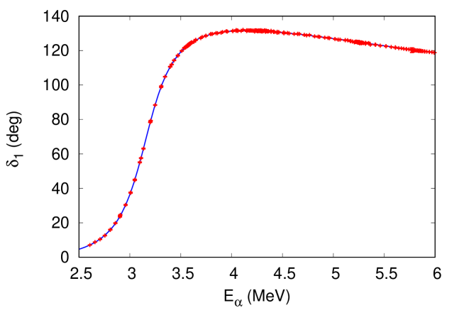
Figure 3: Phase shift, $\delta_{1}$, plotted by using the fitted effective range parameters, $r_{1}$, $P_{1}$, $Q_{1}$ as a function of $E_{\alpha}$. The experimental phase shift data are also displayed in the figure.

Because the energy range is over the energy of $1_{2}^{-}$ state, $E=2.43$ MeV ($E_{\alpha}=3.23$ MeV) and below that of $1_{3}^{-}$ state, $E=5.29$ MeV ($E_{\alpha}=7.05$ MeV), our result indicates that the expression of the effective range expansion given in Eq. (11) is reliable to describe the $1_{1}^{-}$ and $1_{2}^{-}$ states up to $E_{\alpha}=6.0$ MeV.

$r_{C}$ (fm)	$h^{(1)R}\times 10^{4}$ (MeV3)	$y^{(0)}$ (MeV-1/2)	$\chi^{2}/d.o.f$	$S_{E1}$ (keV b)
0.01	$5.2684(11)$	0.253(9)	1.691	60.3(18)
0.035	$2.4483(11)$	0.310(11)	1.697	59.8(18)
0.05	$1.5294(11)$	0.347(12)	1.700	59.3(18)
0.1	$-0.0695(11)$	0.495(18)	1.715	57.9(17)
0.2	$-1.1909(11)$	0.943(34)	1.763	53.6(15)
0.35	$-1.7106(12)$	2.249(84)	1.926	42.1(10)

Table 1: Fitted values of the coupling constants, $h^{(1)R}$ and $y^{(0)}$, to experimental data of $S_{E1}$ at $E=0.9-3$ MeV with the cutoff $r_{C}=0.01-0.35$ fm. The number of the data is $N=151$. The values in the fourth column are $\chi^{2}/d.o.f.$ of the fittings, and those in the last column are our results of $S_{E1}$ at $E_{G}=0.3$ MeV.

We fit the parameters, $h^{(1)R}$ and $y^{(0)}$, to the experimental data of $S_{E1}$ at the energy range, $E=0.9-3.0$ MeV using some values of the cutoff $r_{C}$ in the range, $r_{C}=0.01-0.35$ fm, in the $r$ integral in $X^{(l=1)}_{(d+e)}$ in Eq. (7). The number of the data is $N=151$. In Table 1, we display fitted values of $h^{(1)R}$ and $y^{(0)}$ along with $\chi^{2}/d.o.f$ and our estimate of $S_{E1}$ at $E_{G}$. The uncertainties of the fitted values of $h^{(1)R}$ and $y^{(0)}$ stem from those of the experimental data. We find a significant cutoff dependence of the couplings, $h^{(1)R}$ and $y^{(0)}$, and the $S_{E1}$ factor at $E_{G}$ in the table when varying the short range cutoff, $r_{C}=0.01-0.35$ fm; as the values of $r_{C}$ become larger, the $\chi^{2}/d.o.f.$ become larger while the $S_{E1}$ values become smaller. One may also see that the variation of the $S_{E1}$ factor becomes stable at the cutoff values smaller than $r_{C}=0.1$ fm where the $\chi^{2}/d.o.f$ remain in stable and smaller values. In Fig. 4, we plot a curve of $S_{E1}$ calculated by using the fitted parameters at $r_{C}=0.1$ fm. We display the experimental data and our result of $S_{E1}$ at $E_{G}$ to be mentioned below in the figure as well. One can see that the theory curve reproduces well the experimental data.

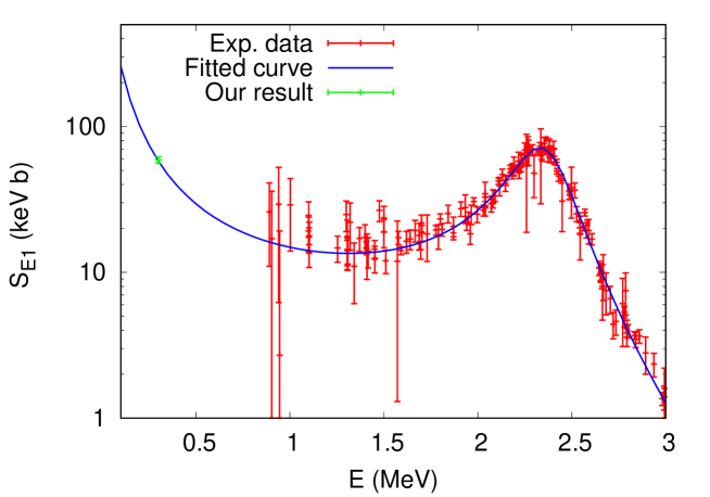
Figure 4: $S_{E1}$ factor plotted by using the fitted parameters with $r_{C}=0.1$ fm as a function of $E$. The experimental data and our estimate of $S_{E1}$ at $E_{G}$ are also displayed in the figure.

In the present work, we choose the results of $S_{E1}$ with $\chi^{2}/d.o.f\simeq 1.7$, in the cutoff region of the stability of $S_{E1}$, for our estimate of $S_{E1}$ at the Gamow-peak energy, $E_{G}=0.3$ MeV, thus, we have

$$S_{E1}=59\pm 3\,\ \mbox{\rm keV$\cdot$b}\,,$$ (19)

where the small, about 5%, uncertainty stems from those of $h^{(1)R}$ and $y^{(0)}$ in Table 1 as well as that of the $r_{C}$ dependence of $S_{E1}$ within $\chi^{2}/d.o.f.\simeq 1.7$. The previous estimates of the $S_{E1}$ factor at $E_{G}$ are well summarized in Table IV in Ref. [5]. The reported vales are scattered from 1 to 340 keV$\cdot$b with various size of the error bars. Nonetheless it is worth pointing out that our result is about 30% smaller than those reported recently: $86\pm 22$ by Tang et al. (2010) [53], 83.4 by Schurmann et al. (2012) [54], $100\pm 28$ by Oulebsir et al (2012) [55], $80\pm 18$ by Xu et al. (2013) [10], $98.0\pm 7.0$ by An et al. (2015) [11], and 86.3 by deBoer et al. (2017) [5].

Regarding the theoretical uncertainty of the present calculation, as discussed above, the non-pole amplitude $X_{(a+b)}^{(l=1)}$ is suppressed and gives less than one percent correction to $S_{E1}$ at $E_{G}$. In the other amplitudes, $X_{(c)}^{(l=1)}$, $X_{(d+e)}^{(l=1)}$, and $X_{(f)}^{(l=1)}$, we find that $X_{(d+e)}^{(l=1)}$ and $X_{(c+f)}^{(l=1)}(=X_{(c)}^{(l=1)}+X_{(f)}^{(l=1)}$) have different momentum dependence and are considerably cancelled with each other. We have $|(X_{(c+f)}^{(l=1)}+X_{(d+e)}^{(l=1)})/X_{(c+f)}^{(l=1)}|=0.055-0.023$ at $E=0.1-3$ MeV; the result is almost linearly decreasing as a function of $E=p^{2}/(2\mu)$. It implies that a higher order correction at N³LO effectively exists in $X_{(d+e)}^{(l=1)}$ while those two contributions, $X_{(c+f)}^{(l=1)}$ and $X_{(d+e)}^{l=1)}$, at LO+NLO and N³LO equally play a significant role to reproduce the $S_{E1}$ data. Though we have not studied a complete set of the corrections at N³LO, a next higher order correction appears at N⁵LO (because a momentum $\vec{p}$ is vector, but a correction should be scalar, $p^{2}$). Thus the higher order correction at N⁵LO which we do not have in the present work may give a few percent correction, $(Q/\Lambda_{H})^{4}\simeq 0.012$, to the estimate of $S_{E1}$ at $E_{G}$.

6. Results and discussion

In this work, we have applied a framework of EFT to the study of radiative $\alpha$ capture on ¹²C for the first time. We have derived the radiative capture amplitudes up to NLO in the standard counting rules, and discussed a modification of the counting rules for the radiative capture amplitudes because of the enhancement of the $p$-wave dressed composite propagator of ¹⁶O. We find that the non-pole amplitude $X_{(a+b)}^{(l=1)}$ is significantly suppressed in the present study. After taking the modification into account, approximately two independent structures (momentum dependence) remain in the amplitudes, $X_{(c+f)}^{(l=1)}$ and $X_{(d+e)}^{(l=1)}$, and we have two unknown parameters in the amplitudes. The two parameters are fitted to the experimental $S_{E1}$ data at $E=0.9-3.0$ MeV, and we find the $S_{E1}$ factor, $S_{E1}=59\pm 3$ keV$\cdot$b at $E_{G}$. Our result is about 30% smaller than the recent estimates, though we have not examined a convergence of our result yet.

A unique feature of EFT is that one can control a theoretical uncertainty of a physical quantity in theory. In the present work, however, we do not examine a convergence of the perturbative expansion of the amplitudes in the estimate of the $S_{E1}$ factor because we did not include a complete set of the higher order corrections. Thus it is important to study higher order corrections to the radiative capture amplitude up to the $Q^{4}$ order to check the convergence of the expansion series and estimate a theoretical uncertainty of $S_{E1}$ at $E_{G}$. Nonetheless, to accurately fix additional parameters, when one includes higher order terms, may not be straightforward due to the present quality of the experimental data set of $S_{E1}$. It might be better studying the other quantities at low energies, such as the $\beta$-delayed $\alpha$ emission spectrum of ¹⁶N or the $\gamma$ angular distribution of the radiative $\alpha$ capture process by employing the present EFT approach.

Acknowledgements

The author would like to thank Kyungsik Kim, Young-Ho Song, Youngman Kim, and Renato Higa for useful discussions. This work was supported by the Basic Science Research Program through the National Research Foundation of Korea funded by the Ministry of Education of Korea (Grant No. NRF-2016R1D1A1B03930122) and in part by the National Research Foundation of Korea (NRF) grant funded by the Korean government (Grant No. NRF-2013M7A1A1075764 and NRF-2016K1A3A7A09005580

References

- [1] W. A. Fowler, Rev. Mod. Phys. 56, 149 (1984).
- [2] L. R. Buchmann and C. A. Barnes, Nucl. Phys. A 777, 254 (2006).
- [3] A. Coc, F. Hammache, J. Kiener, Eur. Phys. J. A 51, 34 (2015).
- [4] C. A. Bertulani and T. Kajino, Prog. Part. Nucl. Phys. 89, 56 (2016).
- [5] R. J. deBoer et al., Rev. Mod. Phys. 89, 035007 (2017), and references therein.
- [6] P. Descouvemont, D. Baye, and P.-H. Heenen, Nucl. Phys. A 430, 426 (1984).
- [7] K. Langanke and S. E. Koonin, Nucl. Phys. A 439, 384 (1985).
- [8] A. M. Lane and R. G. Thomas, Rev. Mod. Phys. 30, 257 (1958).
- [9] J. Humblet, P. Dyer, and B. A. Zimmerman, Nucl. Phys. A 271, 210 (1976).
- [10] Y. Xu et al., Nucl. Phys. A 918, 61 (2013).
- [11] Z.-D. An et al., Phys. Rev. C 92, 045802 (2015).
- [12] P. F. Bedaque and U. van Kolck, Ann. Rev. Nucl. Part. Sci. 52, 339 (2002).
- [13] E. Braaten and H.-W. Hammer, Phys. Rept. 428, 259 (2006).
- [14] U.-G. Meißner, Phys. Scripta 91, 033005 (2016).
- [15] H.-W. Hammer, C. Ji, D.R. Phillips, J. Phys. G 44, 103002 (2017).
- [16] G. Rupak, Nucl. Phys. A 678, 405 (2000).
- [17] S. Ando, R. H. Cyburt, S. W. Hong, C. H. Hyun, Phys. Rev. C 74, 025809 (2006).
- [18] X. Kong and F. Ravndal, Nucl. Phys. A 656, 421 (1999).
- [19] M. Butler, J.-W. Chen, Phys. Lett. B 520, 87 (2001).
- [20] S. Ando, J. W. Shin, C. H. Hyun, S. W. Hong, K. Kubodera, Phys. Lett. B 668, 187 (2008).
- [21] J.-W. Chen, C.-P. Liu, S.-H. Yu, Phys. Lett. B 720, 385 (2013).
- [22] R. Higa, G. Rupak, A. Vaghani, Eur. Phys. J. A 54, 89 (2018).
- [23] X. Zhang, K. M. Nollett, and D. R. Phillips, arXiv:1811.07611 [nucl-th] (2018).
- [24] X. Zhang, K. M. Nollett, and D. R. Phillips, Phys. Rev. C 89, 051602(R) (2014).
- [25] E. Ryberg, C. Forssén, H.-W. Hammer, L. Platter, Eur. Phys. J. A 50, 170 (2014).
- [26] S.-I. Ando, Eur. Phys. J. A 52, 130 (2016).
- [27] S.-I. Ando, Phys. Rev. C 97, 014604 (2018).
- [28] S.-I. Ando, J. Korean Phys. Soc. 73, 1452 (2018).
- [29] T. Teichmann, Phys. Rev. 83, 141 (1951).
- [30] S. R. Beane, M. J. Savage, Nucl. Phys. A 694, 511 (2001).
- [31] S. Ando, C. H. Hyun, Phys. Rev. C 72, 014008 (2005).
- [32] S. Ando, J. W. Shin, C. H. Hyun, S. W. Hong, Phys. Rev. C 76, 064001 (2007).
- [33] S.-I. Ando, Eur. Phys. J. A 33, 185 (2007).
- [34] E. Ryberg, C. Forssén, H.-W. Hammer, and L. Platter, Phys. Rev. C 89, 014325 (2014).
- [35] S.-I. Ando and C. H. Hyun, Phys. Rev. C 86, 024002 (2012).
- [36] T. Fuchs, J. Gegelia, G. Japaridze, and S. Scherer, Phys. Rev. D 68, 056005 (2003).
- [37] S. Ando and H. W. Fearing, Phys. Rev. D 75, 014025 (2007).
- [38] D. Baye and E. M. Tursunov, J. Phys. G: Nucl. Part. Phys. 45, 085102 (2018).
- [39] P. Descouvemont and D. Baye, Phys. Lett. B 127, 286 (1983).
- [40] P. Descouvemont and D. Baye, Nucl. Phys. A 459, 374 (1986).
- [41] P. Descouvemont and D. Baye, Phys. Rev. C 36, 1249 (1987).
- [42] D. Foreman-Mackey et al., arXiv:1202.3665v4 [astro-ph.IM] (2013).
- [43] P. Tischhauser et al., Phys. Rev. C 79, 055803 (2009).
- [44] P. Dyer and C. Barnes, Nucl. Phys. A 233, 495 (1974).
- [45] A. Redder et al., Nucl. Phys. A 462, 385 (1987).
- [46] J. M. L. Ouellet et al., Phys. Rev. C 54, 1982 (1996).
- [47] G. Roters et al., Eur. Phys. J. A 6, 451 (1999).
- [48] L. Gialanella et al., Eur. Phys. J. A 11, 357 (2001).
- [49] R. Kunz et al., Phys. Rev. Lett. 86, 3244 (2001).
- [50] M. Fey, Ph.D. thesis (Universitat Stuttgart) (2004).
- [51] H. Makii et al., Phys. Rev. C 80, 065802 (2009).
- [52] R. Plag et al., Phys. Rev. C 86, 015805 (2012).
- [53] X. D. Tang et al., Phys. Rev. C 81, 045809 (2010).
- [54] D. Schurmann et al., Phys. Lett. B 711, 35 (2012).
- [55] N. Oulebsir et al., Phys. Rev. C 85, 035804 (2012).