Inference Trees: Adaptive Inference with Exploration

Abstract

We introduce inference trees (ITs), a new class of inference methods that build on ideas from Monte Carlo tree search to perform adaptive sampling in a manner that balances exploration with exploitation, ensures consistency, and alleviates pathologies in existing adaptive methods. ITs adaptively sample from hierarchical partitions of the parameter space, while simultaneously learning these partitions in an online manner. This enables ITs to not only identify regions of high posterior mass, but also maintain uncertainty estimates to track regions where significant posterior mass may have been missed. ITs can be based on any inference method that provides a consistent estimate of the marginal likelihood. They are particularly effective when combined with sequential Monte Carlo, where they capture long-range dependencies and yield improvements beyond proposal adaptation alone.

1 Introduction

The choice of proposal distribution is a key factor in the performance of Monte Carlo (MC) methods. Unfortunately, it is typically difficult to know what constitutes a good proposal prior to performing inference. For this reason, many methods use past samples to adapt the proposal at future iterations [10, 13, 14, 21, 24], for example by minimizing the KL divergence between the empirical distribution over samples and the proposal. These strategies implicitly assume that preceding samples are representative of the true posterior. This leads to the somewhat undesirable characteristic that we already need good samples to have effective adaptation, which is presumably difficult to achieve given our need to adapt in the first place. Adaptive methods can consequently exhibit pathologies, such as collapsing to a single mode or even adapting to invalid proposals [3, 11].

To address these issues, we propose that adaptive methods should not only carry out exploitation, that is sample in regions where we believe the posterior mass is high, but also exploration, that is explicitly invest computational resources to sample in regions where our current uncertainty about the posterior mass is high. In other words, we should recognize that the utility derived from the generated samples originates not only from their direct contribution to the estimator, but also the degree to which they inform future sampling.

To this end, we introduce inference trees (ITs), a new class of adaptive methods that build on ideas from Monte Carlo tree search (MCTS) [8, 23]. ITs hierarchically partition the parameter space into disjoint regions in an online manner, resulting in more fine-grained partitions for regions where the posterior density is large. This transforms the problem of inference on the full parameter space to a set of constrained inference problems, which we can combine in a manner akin to stratified sampling [12, 28]. By adaptively choosing regions in which to refine our estimates, we can explicitly control the exploration-exploitation trade-off. This results in an algorithm that can expend computational resources to investigate whether the proposal can be improved, for example by searching for missing modes, rather than just greedily exploiting the best proposal learned so far.

ITs can be thought of as a meta-algorithm that controls the allocation of computational resources of a base inference algorithm. We show that, under mild assumptions, ITs define a consistent estimator whenever the base algorithm itself provides a consistent estimator. This property is independent of the methods for learning the partitioning and allocation of computational resources between the partitions. In addition to the theoretical guarantees that this provides, the resulting flexibility proves critical to the empirical performance of ITs. For example, we exploit this flexibility to introduce a novel allocation scheme that uses targeted exploration: rather than just using an optimism boost [5] to ensure a minimum level of allocation for all regions, it uses explicit uncertainty estimates for the true marginal posterior mass of a region to identify important areas to explore, such as those likely to contain a missing mode. Underlying this approach is a novel estimator in its own right. Namely, we perform density estimation on sample weights to predict the probability the true marginal posterior mass of a region is above a certain threshold. Remarkably, this estimator remains robust even when the MC estimate of the marginal is thousands of orders of magnitude smaller than the true value.

We find that the gains that ITs provide are particularly pronounced when they are combined with sequential Monte Carlo (SMC) [16], where they offer a means of capturing long-range dependencies. This yields improvements beyond what can be achieved by the so-called one-step optimal proposal.

2 Background and Related Work

Our aim is to approximate a target density $\pi(x)=\gamma(x)/\omega$, for which it is possible to evaluate the unnormalized density $\gamma(x)$ pointwise, but computation of the normalization constant $\omega$ is intractable. We will assume that we have a base MC algorithm that returns weighted samples and makes use of some form of proposal distribution $q(x)$. Though we will later consider other approaches (see §7.2), for exposition, it will be easiest to think of this base algorithm as being self-normalized importance sampling [29], which defines an estimated measure based on weighted samples from $q$,

$$\hat{\pi}(\cdot):=\sum_{n=1}^{N}\bar{w}_{n}\delta_{\hat{x}^{n}}(\cdot)\quad\text{where}\quad\hat{x}^{n}\sim q(x),\quad\bar{w}_{n} :=\frac{w_{n}}{\sum_{n=1}^{N}w_{n}},\quad w_{n}:=\frac{\gamma(\hat{x}^{n})}{q(\hat{x}^{n})}.$$ (1)

2.1 Adaptive Monte Carlo Inference

Though there are a range of approaches for adapting the proposal $q$ (see Bugallo et al. [9] for a review), most share a common framework of alternating between sampling using the current proposal and adapting the proposal using previous samples, with the latter often taking the form of a (potentially implicit) density estimation. For example, one common approach is to, at each iteration, choose the proposal that minimizes the KL divergence from the estimated posterior to the proposal [11, 15]. Namely, if $\theta$ denotes the parameters of $q$, one uses $\theta^{*}=\operatorname*{arg\,\!min}_{\theta}\sum_{n=1}^{N}-\bar{w}_{n}\log q_{\theta}(\hat{x}^{n})$ at each iteration. This leads to an expectation maximization style approach that is greedy, in the sense that past samples are assumed to accurately represent the posterior.

2.2 Multi-Armed Bandits and Monte Carlo Tree Search

In multi-armed bandit problems, an agent sequentially chooses between multiple actions, known as arms, each of which returns a stochastic reward. The agent’s goal is to maximize the long-term cumulative reward [1, 7]. One common strategy is upper confidence bounding (UCB) [5], which chooses the arm $j$ that maximizes the utility

$$u_{j}=\hat{r}_{j}+(\beta/\sqrt{M_{j}})\log\textstyle\sum\nolimits_{i}M_{i}.$$ (2)

In this definition, $\hat{r}_{j}\in[0,1]$ is the current estimate of the expected reward for each arm, $M_{j}$ is the number of times arm $j$ was previously pulled, and $\beta$ is a parameter that controls the level of exploration. Here $\hat{r}_{j}$ is an exploitation term that ensures we pull arms with high expected reward more frequently, while $(\beta/\sqrt{M_{j}})\log\textstyle\sum\nolimits_{i}M_{i}$ is an exploration term, sometimes known as an optimism boost, which encourages us to pull arms which have been pulled infrequently so far.

Of particular relevance to our work is the study of bandits in the stratified sampling setting [12, 19, 20, 22, 27]. Here one splits a target integral into a number of strata, then looks to minimize the overall error by allocating samples to the MC estimators associated with each strata. The optimal strategy can be shown to sample each strata in proportion to the standard deviation of its evaluations [12]. Because one now needs to asymptotically sample from each arm infinitely often, the strategy is adjusted to

$$u_{j}=\left(\hat{r}_{j}+(\beta/\sqrt{M_{j}})\log\textstyle\sum\nolimits_{i}M_{i}\right)/M_{j}$$ (3)

where $\hat{r}_{j}$ is typically set to the empirical standard deviation. ITs differ from these approaches in that they use hierarchical stratification, learn this stratification in an online manner, use a different utility that incorporates a targeted exploration term, and adapt UCB to the inference setting.

MCTS [8, 23] uses a hierarchy of arms where one traverses the tree by sequentially choosing child nodes using (2) (or a variation thereof) until a leaf is reached, then refines that node and propagates the new estimates up through the tree. The average reward $\hat{r}_{j}$ of a non-leaf node is the average of those of its children, while $M_{j}$ becomes the number of times a node has been traversed. MCTS has traditionally been used for planning [32] and in discrete decision settings. We believe that our work is the first to consider MCTS in the context of inference or integration, as opposed to optimization. ITs also vary from the standard MCTS setting in how rewards are calculated and propagated.

3 Algorithm Overview

ITs hierarchically partition the target space, run inference separately on the resulting disjoint regions to obtain local estimates, and then combine these local estimates into one overall estimate. Each node in the tree corresponds to a region of target space, $A_{j}$, such that the region of a parent node is the union of its children, $A_{j}=A_{\ell_{j}}\cup A_{r_{j}}$ where $\ell_{j}$ and $r_{j}$ are the child indices, and the union of all leaf nodes is the full space. We assume that we are able to sample from the proposal restricted to a node, $q(x|x\in A_{j})$, and evaluate this renormalized truncated density pointwise. How this is achieved is discussed in §4.1. The IT learning process can be broken down into three components as follows.

Traversal: The traversal step adaptively allocates computational resources to areas of the target space, balancing exploration and exploitation to minimize the error of our final overall estimate. Following similar lines to MCTS, it starts at the root node and then recursively choosing a child node until a leaf is reached. To choose between children, we use the stratified sampling UCB formulation given in (3). However, as we explain in detail §5, our $\hat{r}_{j}$ will vary from standard settings: our reward must be adapted to reflect the fact we are doing inference and rather than relying solely on the optimism boost for exploration, we will incorporate a targeted exploration term.

Refinement: In the refinement step we improve the estimate at the chosen node, either by running inference directly and updating the local estimate, or expanding the tree by splitting the node and running inference at each of the generated child nodes. For both cases, the inference itself is performed using the base algorithm and the truncated proposal $q\left(x\mid x\in A_{j}\right)$. The two considerations for refinement are whether to split and how to split. They are discussed in §6.

Propagation: In the propagation step, we recursively update the tree with the new estimates produced by the refinement step, starting with the refined node(s) and then updating all their ancestors. This improves our posterior representation and guides the future traversal strategy. Along with a small number of additional terms required for the traversal, two key quantities are propagated up through the tree: a marginal likelihood estimate $\hat{\omega}_{j}$ and an unnormalized empirical measure $\hat{\gamma}_{j}(\cdot)$. The truncated posterior approximation at any node in the tree is then given by the self-normalized estimated measure $\hat{\pi}_{j}(\cdot)=\hat{\gamma}_{j}(\cdot)/\omega_{j}$, with the root note estimate $\hat{\pi}_{0}(\cdot)$ representing our overall approximation. The specifics of the propagation are discussed in §4.

Putting these components together leads to an adaptive online inference algorithm as summarized in Algorithm 1. We now discuss the individual elements of ITs in more detail. We note that, while the method for propagation is tightly coupled with the IT estimator itself, the consistency of this estimator is independent of the traversal and refinement strategies. Consequently, a wide range of possible approaches fall under the general IT framework we have just introduced.

Algorithm 1 Inference Tree Training

1:Unnormalized target density $\gamma(x)$, “truncatable” proposal $q(x)$, base inference algorithm $\mathcal{F}$, complete target space $A_{0}$, number of iterations to run $R$, batch size $b$, existing tree $\mathcal{T}$ (optional)

2:Inference Tree $\mathcal{T}$, posterior empirical measure $\hat{\pi}_{0}(\cdot)$

3:If required, initialize tree $\mathcal{T}$ by running inference on full space $\left\{\hat{x}_{0}^{n},w_{0}^{n}\right\}_{n=1}^{b}\leftarrow\mathcal{F}\left(\gamma(x),q\left(x|A_{0}\right),b\right)$

4:for $r=1:R$ do

5:     Traverse tree by recursively selecting the child with highest $u_{j}$ (see (6)) until a leaf $(j)$ is reached

6:     if decide to split node $j$ then $\triangleright$ See §6

7:         Use existing samples to split node $A_{\ell_{j}},A_{r_{j}}\leftarrow A_{j}$ where $A_{j}=A_{\ell_{j}}\cup A_{r_{j}}$ $\triangleright$ See §4.1 and §6

8:         $\{\hat{x}_{\ell_{j}}^{n},w_{\ell_{j}}^{n}\}_{n=1}^{b}\leftarrow\mathcal{F}\left(\gamma(x),q\left(x|A_{\ell_{j}}\right),b\right)$,  $\{\hat{x}_{r_{j}}^{n},w_{r_{j}}^{n}\}_{n=1}^{b}\leftarrow\mathcal{F}\left(\gamma(x),q\left(x|A_{r_{j}}\right),b\right)$

9:     else  Run further inference on current node $\left\{\hat{x}_{j}^{n},w_{j}^{n}\right\}_{n=N_{j}+1}^{N_{j}+b}\leftarrow\mathcal{F}\left(\gamma(x),q\left(x|A_{j}\right),b\right)$   end if      

10:     Update $\hat{\gamma}_{j}(\cdot)$ and $\hat{\omega}_{j}$ for refined node(s) and all ancestors using (5a) and (5b) respectively   end for

11:Return tree $\mathcal{T}$ and self normalized empirical measure $\hat{\pi}_{0}(\cdot)\leftarrow\hat{\gamma}_{0}(\cdot)/\hat{\omega}_{0}$

4 The Inference Tree Estimator

Assume we are trying to estimate the expectation of a measurable function $f(x)$ with respect to the target measure $\pi(x)$. For any set of disjoint regions $\{A_{i}\}_{i\in\mathcal{I}}$ covering the full target space, we have

$$\mathbb{E}_{\pi(x)}[f(x)] =\frac{1}{\omega}\int\gamma(x)f(x)\,dx=\frac{1}{\omega}\int\gamma(x)f(x)\sum_{i\in\mathcal{I}}\mathbb{I}(x\in A_{i})\,dx=\frac{\sum_{i\in\mathcal{I}}\mathbb{E}_{q\left(x\mid A_{i}\right)}\left[\frac{\gamma(x)f(x)}{q\left(x\mid A_{i}\right)}\right]}{\sum_{i\in\mathcal{I}}\mathbb{E}_{q\left(x\mid A_{i}\right)}\left[\frac{\gamma(x)}{q\left(x\mid A_{i}\right)}\right]}$$

$$\approx\frac{\sum_{i\in\mathcal{I}}\frac{1}{N_{i}}\sum_{n=1}^{N_{i}}w_{i}^{n}f(\hat{x}_{i}^{n})}{\sum_{i\in\mathcal{I}}\frac{1}{N_{i}}\sum_{n=1}^{N_{i}}w_{i}^{n}}\quad\text{where}\quad\hat{x}_{i}^{n}\sim q(x|A_{i}),\quad w_{i}^{n}:=\frac{\gamma(\hat{x}_{i}^{n})}{q(\hat{x}_{i}^{n}|A_{i})}.$$ (4)

We now see that we can calculate estimates separately for each region $A_{i}$ and then combine these in an unweighted manner – there are no correction factors for the strategy used to assign computational resources. However, we emphasize that there are two key reasons that we are able to do this. Firstly, rather than locally self-normalizing, we separately combine unnormalized target estimates and an estimate for the normalization constant, and then globally self-normalize the estimate. Secondly, the truncated proposals $q(x|A_{i})$ are correctly normalized such that $\int_{x\in A_{i}}q(x|A_{i})dx=1$.

In practice, we often do not know $f(x)$ at inference time. However, we can always compute empirical measures based on weighted samples $\frac{1}{N_{i}}\sum_{n=1}^{N_{i}}w_{i}^{n}\delta_{\hat{x}_{i}^{n}}(\cdot)$, which can then later be used to evaluate any target function as and when required.

Though the leaves of an inference tree form a suitable disjoint partitioning of the target space, we also have access to local estimates from non-leaf nodes, left over from when those nodes were previously leaves themselves. The IT estimator is therefore constructed recursively, such that the estimate at any node is a combination of its child estimates and this local estimate; the propagation step of the algorithm corresponds to online updates of these estimates. To combine estimates from parents with the children, we introduce a preference factor to the estimator from the child nodes, $c_{j}\in[0,1]$, and define the IT estimator for node $j$ recursively using

$$\hat{\pi}_{j}\left(\cdot\right):=\frac{\hat{\gamma}_{j}(\cdot)}{\hat{\omega}_{j}},\quad\text{where}\quad\hat{\gamma}_{j}(\cdot) :=\frac{(1-c_{j})}{N_{j}}\sum\nolimits_{n=1}^{N_{j}}w_{j}^{n}\delta_{\hat{x}^{n}_{j}}(\cdot)+c_{j}\left(\hat{\gamma}_{l_{j}}(\cdot)+\hat{\gamma}_{r_{j}}(\cdot)\right),$$ (5a)

$$\hat{\omega}_{j} :=\frac{(1-c_{j})}{N_{j}}\sum\nolimits_{n=1}^{N_{j}}w_{j}^{n}+c_{j}\left(\hat{\omega}_{l_{j}}+\hat{\omega}_{r_{j}}\right),$$ (5b)

$\ell_{j}$ and $r_{j}$ refer to the child node indices, and our overall estimate is given by that of the root node $\hat{\pi}_{0}\left(\cdot\right)$. For leaves, $c_{j}=0$, such that we simply take the local estimate. For internal nodes, let $M_{j}$ denote the total number of samples drawn at that node or any of its descendants. We then define $c_{j}=\chi_{j}(M_{j}-N_{j})/M_{j}$ (such that $(M_{j}-N_{j})/M_{j}$ is the proportion of the samples that are from the children) and $\chi_{j}$ is an additional factor to account for the fact that the child estimate will generally be more efficient than the parent (see Appendix C). Critically, $c_{j}\to 1$ as $M_{j}\to\infty$ for a fixed $N_{j}$.

The IT approach is backed up by the following consistency result in the number of IT iterations.

Theorem 1.

If the following hold as the number of IT iterations becomes infinitely large

• The total number of leaf nodes remains bounded and each is visited infinitely often;

• When provided with an infinite sample budget and an arbitrary subregion $A$ generated by the node splitting procedure, the base inference algorithm produces an empirical measure $\hat{\gamma}(\cdot)$ and normalization constant estimate $\hat{\omega}$ which respectively converge weakly to $\gamma(x)\mathbb{I}(x\in A)$ and converge in probability to $\int_{x\in A}\gamma(x)dx$;

then each $\hat{\pi}_{j}(\cdot)$ as defined by (5) converges weakly to $\pi(x|x\in A_{j})$ and, in particular, $\hat{\pi}_{0}(\cdot)$ converges weakly to $\pi(x)$.

The proof is given in Appendix B. We see that, subject to mild assumptions, consistency is achieved regardless of our traversal and refinement strategies. Inevitably, however, these will affect the practical performance. In the following, we now develop effective strategies for each component in turn.

4.1 Partitioning the Target Space

Directly partitioning in the space of $x$ can be challenging. Typically it will not be desirable for the partitions to be axis-aligned (or even linear). Conversely, it is in general not possible to evaluate the partitioned proposal $q(x|A_{j})$ for arbitrary $A_{j}$. To address this, ITs use a reparameterization of the proposal, such that $x=g(z_{1:T})$ where $z_{1:T}$ is uniformly distributed on the unit hypercube $[0,1]^{T}$. Though this is not always exactly the case, $g$ can generally be thought of as an inverse cumulative distribution function of $q(x)$ (with $T$ set to the dimensionality of $x$). ITs use axis-aligned partitions in the space of $z_{1:T}$, which in turn induce (typically nonlinear) partitions on $x$. The motivation for this is twofold. Firstly, because the distribution is uniform over $z_{1:T}$, this eliminates the problem of trying to choose splits that align well with the contours of $q$. Secondly, it means that we can easily sample from and evaluate $q(x|A_{j})$: $A_{j}$ will always represent a hyperrectangle $B_{j}$ in the space of $z_{1:T}$, so we can sample from $q(x|A_{j})$ by sampling uniformly from $B_{j}$ and passing the samples through $g$, while $q(x|A_{j})=q(x)\mathbb{I}(x\in A_{j})/\lVert B_{j}\rVert$ where $\lVert B_{j}\rVert$ is the volume of this hyperrectangle, leading to simple evaluation as required by the importance weight evaluations. See Appendix A for further discussion.

5 Traversal Strategy

As explained in §3, the traversal strategy starts at the root node and then recursively chooses the child node with the higher utility $u_{j}$ until a leaf node is reached. Though we will use a utility of the UCB form given in (3), our reward estimate $\hat{r}_{j}$ will reflect both the need for exploitation and exploration, unlike in standard approaches where it represents only exploitation.

We start by quoting our final choice for the utility, before explaining each of the component terms in detail. Using $\text{pa}(j)$ and $\text{si}(j)$ to denote the parent and sister of node $j$ respectively, we have

$$u_{j}=\frac{1}{M_{j}}\Bigg{(}\left(1-\delta\right)\left(\frac{\hat{\tau}_{j}}{\hat{\tau}_{\text{pa}(j)}}\right)^{\left(1-\alpha\right)}+\delta\frac{\hat{p}^{s}_{j}}{\hat{p}^{s}_{j}+\hat{p}^{s}_{\text{si}(j)}}+\beta\frac{\lVert B_{j}\rVert}{\lVert B_{\text{pa}(j)}\rVert}\frac{\log M_{\text{pa}(j)}}{\sqrt{M_{j}}}\Bigg{)}$$ (6)

Here $\hat{\tau}_{j}$ estimates the optimal asymptotic rate for sampling the node (see (7)), while $\hat{p}^{s}_{j}$ is a subjective probability estimate for the node containing significant posterior mass (see (9)). Consequently, the first and second terms encourage exploitation and targeted exploration respectively, with $\delta\in[0,1]$ being a parameter that controls the relative emphasis. We will typically reduce $\delta$ over time to encourage more exploitation, along with $\alpha\in[0,1]$, an annealing parameter that encourages sampling of the tails. The different normalizations for $\hat{\tau}_{j}$ and $\hat{p}^{s}_{j}$ originate from the fact that we want the exploration term to dominate whenever $\hat{\tau}_{\text{pa}(j)}\gg\hat{\tau}_{j}+\hat{\tau}_{\text{si}(j)}$, implying that the children have underestimated the exploitation target. The last term is a classical optimism boost [5], with the exception that it is scaled by the relative volume of the node $\lVert B_{j}\rVert/\lVert B_{\text{pa}(j)}\rVert$. We now discuss $\hat{\tau}_{j}$ and $\hat{p}^{s}_{j}$ in detail.

5.1 Exploitation Target

To derive our exploitation target, $\tau_{j}$, we ask the question: what is the asymptotically optimal rate for allocating samples to regions? In other words, if all our node estimates were perfect, how should we allocate our samples? One might intuitively expect that the answer to this would be to allocate samples in proportion to the marginal probability mass of a region. However, it turns out that this is not the case: the variance on the weights is different for different regions and so we also need to sample more from regions where this variance is high. In fact, as we show in Appendix D, the optimal allocation strategy is to sample according to

$$\tau_{j}=\sqrt{\omega_{j}^{2}+(1+\kappa)\sigma_{j}^{2}}$$ (7)

where $\sigma_{j}^{2}$ is the variance of the weights (as produced by single traversal) and $\omega_{j}$ is the marginal posterior mass of the region as before. Here $\kappa\in[0,\infty]$ is a “smoothness” parameter, which dictates the relative importance of the two terms when using the generated samples to estimate a particular expectation as per (4). For example, $\kappa\to\infty$ corresponds to the optimal setup for estimating the marginal likelihood, for which $f(x)=1$ is completely flat.

To estimate $\tau_{j}$, we use $\hat{\tau}_{j}=\sqrt{\hat{\omega}_{j}^{2}+(1+\kappa)\hat{\sigma}_{j}^{2}}$ with propagated estimates $\hat{\omega}_{j}$ and $\hat{\sigma}_{j}^{2}$. The former is given by (5b), while the latter requires a distinct propagation scheme as discussed in Appendix D.

5.2 Targeted Exploration through Density Estimation of the log Weights

Relying only on the optimism boost for exploration, as done by standard UCB schemes, can be chronically inefficient in practice as it only encourages a uniform exploration. We, therefore, introduce a targeted exploration term into our utility, $\hat{p}_{j}^{s}$, which provides a subjective probability estimate for the event that the region contains significant posterior mass that we have thus far missed.

Providing such a reliable estimate is a challenging problem. Our global proposal $q(x)$ is often very poor meaning standard MC estimates can be woefully inadequate: we will consider experiments where we regularly underestimate the marginal likelihood (ML) by factors in excess of $10^{1000}$.

Our insight is that, even when the ML is substantially underestimated, the raw log weights still convey useful information about what the true value could be. We exploit this insight by carrying out density estimation of the log weights and using this as a basis for constructing $\hat{p}_{j}^{s}$. Consider the demonstrative

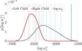
Figure 1: Density estimation for log weights.

example shown in Figure 1 where we want to predict whether the true log ML of each child is above some threshold $\log w_{\text{th}}$. Here we see that there is a high chance that the left child has a true ML above the threshold, but we can be reasonably confident the right does not. Critically, we can make this assertion even though our MC estimates for the ML are underestimated by hundreds of orders of magnitude.

To formalize this intuition, let $\psi(\log w_{j}^{n})$ denote a density estimator for a nodes local weights, with associated cumulative density $\Psi(\log w_{j}^{n})$. The key idea is to use this density estimator to predict the probability that one more samples will exceed a target threshold $\log w_{\text{th}}$ if we were to generate another $T$ “lookahead” samples, where $T$ is some large, but finite, number. When $\log w_{j}^{n}$ varies over a large range, the MC estimate for the ML is effectively equal to the maximum weight, and so we have

$$P\left(\hat{\omega}_{j}(T)>w_{\text{th}}\right)\approx P\left(\max(w_{j}^{1:T})>w_{\text{th}}\right)\approx 1-(1-\Psi(\log w_{\mathrm{th}}))^{T}$$ (8)

where $\hat{\omega}_{j}(T)$ is MC estimate for the ML after taking $T$ samples. Though we could now use this estimate to construct $\hat{p}^{s}_{j}$ directly, we apply a heuristic of scaling by the effective sample size (ESS) [29] of the node (see Appendix D) on the basis that a high ESS suggests that we have already a reasonable ML estimate and thus do not need to explore further.

To complete the picture, we define the propagation strategy for these probability estimates by assuming that the $\hat{p}_{j}^{s}$ are independent for sibling nodes, finally yielding the recursive definition

$$\hat{p}^{s}_{j}:=\left(1-c_{j}\right)\frac{1-(1-\Psi(\log w_{\mathrm{th}}))^{T}}{\text{ESS}_{j}}+c_{j}\left(\hat{p}^{s}_{\ell_{j}}+\hat{p}^{s}_{r_{j}}-\hat{p}^{s}_{\ell_{j}}\hat{p}^{s}_{r_{j}}\right)$$ (9)

analogous to that of $\hat{\omega}_{j}$ in (5b). In our experiments, we found $\log w_{j}^{n}$ was typically well approximated by a Gaussian (there is also theoretical evidence this is appropriate when SMC is used as the base algorithm [6, 18, 30]) and so this simple choice was taken for $\psi$. In cases where this gives a poor fit, one could instead use a kernel density estimator. Setting $T$ and $w_{\text{th}}$ is detailed in Appendix F.2.

6 Refinement Strategy

Once a leaf is chosen by the traversal, there are two ways we can refine the tree: update the local estimate or split the node. The two considerations here are whether to split and how to split.

At a high-level, a good partitioning structure is one in which the posterior mass is concentrated in a small number of regions. In essence, we gain most from being able to “eliminate regions” from consideration, reducing the proportion of the target space that needs to be actively considered. When we propose to split a node, we thus want to find the split that best concentrates the posterior mass. Conveniently, we can use the samples already generated at the node to try and predict what will be a good split. Namely, we can hypothesize a number of splits and then evaluate how well each split will concentrate the mass, based on the existing samples. Though we do not directly use them in this way, ITs indirectly parameterize an importance sampling proposal, whereby we traverse the tree, recursively sampling a child with probability proportional to $\hat{\tau}_{j}$. We can, therefore, measure the concentration of mass through the entropy of this implied proposal.

Recall from §4.1 that ITs use axis-aligned partitions in the reparameterized space $z_{1:T}$ and that our proposal for a leaf node is uniform in this space. We can therefore analytically calculate the entropy of a hypothetical split (see Appendix G) and use this as loss criterion for choosing a split:

$$\textsc{Loss}(\text{split}) =\hat{\omega}_{\ell}\log\frac{\lVert B_{\ell}\rVert}{\hat{\omega}_{\ell}}+\hat{\omega}_{r}\log\frac{\lVert B_{r}\rVert}{\hat{\omega}_{r}}$$ (10)

where the child volumes and marginal probability estimates are implied for any hypothetical split. The lower this loss, the more information our split conveys about where the posterior mass is concentrated. As hypothetical splits can be quickly tested – there is no need to run inference – we can efficiently test out a relatively large number ($\sim 100$) of random splits and then choose the one that minimizes (10). We then initialize the newly generated nodes by running inference separately on each of them.

We further introduce heuristics for whether to split in order to avoid unnecessary over-splitting. Firstly, we only attempt to split once $N_{j}$ reaches a certain threshold and if the ratio $\text{ESS}_{j}/N_{j}$ falls below a certain threshold: we want to stop splitting once a node represents a near perfect sampler. Secondly, whenever we split a node, we check that split passes a usefulness test, namely a significance test that the distributions of the $\log w_{j}$ are different, rejecting the split if this test fails.

7 Experiments

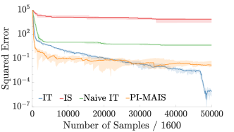
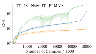
Figure 2: Convergence for the GMM in terms of the log ML estimate (left) and the ESS (right). The ground truth log marginal was estimated using a very large number of samples and a manually adapted proposal. Solid lines represent median over 10 runs and shading the 25%-75% quantiles. The reason for the “just-in-time” style convergence of the IT stems from the fact that the parameter annealing schedules start to kick in and encourage far more exploitation near the end of the runs.

7.1 Gaussian Mixture Model

Our first experiment is to infer the cluster means in a Gaussian mixture model (GMM). Specifically,

$${\mu}_{k}\sim\mathcal{N}({0},\Sigma_{\mu}),\quad\,\,z_{n}\big{|}\ {\pi}\sim\mathrm{Categorical}(\{1/K,\dots,1/K\}),\quad\,\,{y}_{n}\big{|}\ z_{n}=k,{\mu}_{k}\sim\mathcal{N}({\mu}_{k},\Sigma_{y}),$$

where we set $\Sigma_{\mu}={I}$, $\Sigma_{y}=0.2{I}$, and $K=4$. We generated a two-dimensional synthetic dataset ${y}_{1:200}$ using the generative model and then ran ITs with importance sampling as the base algorithm to conduct inference on ${\mu}_{k}$, with the $z_{n}$ marginalized out by summation. We use the prior on ${\mu}_{k}$ as our base proposal. Though simple, this constitutes a surprisingly challenging inference problem, as symmetries in the model mean that the posterior is concentrated in $24$ well-separated modes, each of which occupy less than $10^{-10}$ of the overall eight-dimensional parameter space.

For computational efficiency, we fixed “one run” of the base inference algorithm to be comprised of drawing $100$ importance samples and we undertook $16$ runs of this base algorithm for each refinement step (with each counting as a separate traversal). We further took the convention in, for example, log weight density estimation that each “run” returns a single amalgamated $w_{i}^{n}$, which might itself contain multiple samples (similarly $w_{i}^{n}$ becomes the SMC ML estimate in the next experiment). We compared to the following baselines given the same total budget of target density evaluations: non-adaptive importance sampling; a naïve IT implementation where we set $\delta=0$, $\alpha=0$, and $\beta=0.5$, which means that our target ignores the $\hat{p}_{j}^{s}$ terms and relies solely on the optimism boost for exploration; and PI-MAIS [26], a state-of-the-art adaptive importance sampler based on simulating a large number of Markov chains to construct the proposal. Each algorithm was given a budget of $8\times 10^{7}$ target evaluations, with the parameters set as per Appendix H.

For comparison, we examined the convergence of the ML estimate and ESS (Figure 2) and a kernel density estimator of the final output (Figure 3). The results show that ITs outperformed the alternatives. Unsurprisingly, vanilla importance sampling performed poorly throughout, ending with an ESS of effectively 1. The naïve IT implementation managed to generate a very high ESS, but typically only found two or three modes leading to a substantial error in the ML estimate. PI-MAIS did better at finding modes, though still substantially worse than IT. Further, it ended with a low ESS and produced poor estimates for the relative sizes of the modes, in turn giving an inferior log ML estimate.

7.2 Chaotic Dynamics Model

Dealing with long-range dependencies, i.e. variables that have influence many steps after they are sampled, can be challenging in SMC as variables are often fixed before all dependent terms are incorporated, leading to sample degeneracy. Viewing this in another light, the intermediate target distributions can vary substantially from the target marginal distribution on the relevant variables. Naïve strategies for dealing with this tend to be futile – the resampling step always corrects to the intermediate target and thus incorporating lookahead information in proposals often reduces the effective sample size. In some cases, auxiliary weighting schemes provide a degree of lookahead [17, 25], but these typically entail a substantial increase in computational cost while providing only a short-range lookahead. Moreover, problems with degeneracy can be compounded in the context of adaptation as information is only received for particles that survive the resampling. We now show that ITs can address these challenges by running inference on separate regions. Namely, the IT process allows information to be gathered even in the face of degeneracy. Constraining different sweeps to different regions allows samples to be “forced through” the resampling steps, hereby dealing with long-range dependencies. This is done without losing the key benefits of SMC, as gains from resampling are still seen when running inference within a particular region. Note that ITs only require an unbiased estimate for the weights in a manner akin to pseudo-marginal methods [2], such that we can run SMC when there are some latent variables not directly controlled by the IT.

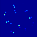
(a) PI-MAIS

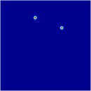
(b) Naïve IT

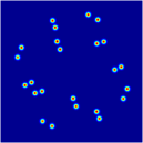
(c) IT

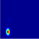
(d) PMMH

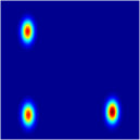
(e) Naïve IT

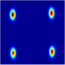
(f) IT

Figure 3: Kernel density estimate of projected posterior estimates for the GMM (a-c) and the chaos model (d-f). We use a linear projection of the original 8/4-dimensional spaces and exaggerate the variance of the modes for visualization purposes. For both problems, the IT has successfully recovered all modes and inferred that all the modes have equal mass. Though the naïve IT implementation produced good estimates for the modes it found, it missed modes for both problems. For the GMM, PI-MAIS found a number of modes but still missed some and misestimated their relative masses. For the chaos model, PMMH only found a single mode.

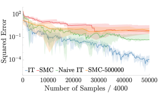
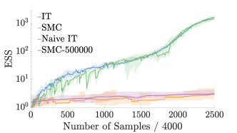
Figure 4: Convergence of log ML and ESS for chaos model, conventions as per Figure 2. PMMH is not shown as it returns unweighted samples and no ML estimate; other results are given in Appendix I.

To test ITs in this setting, we consider an adaptation of the chaotic dynamical system tracking problem introduced by [31], details for which are given in Appendix H. The model comprises of an extended Kalman filter where we have dynamics parameters $\theta$, latents $x_{1:T}$, and observations $y_{1:T}$. We desire to conduct inference over both the dynamics parameters and the latent variables, but will only use ITs to control the sampling of the former. This model contains long-range dependencies because the dynamics parameters affect each transition and so the smoothing marginal $p(\theta|y_{1:T})$ is very different to the filtering marginal $p(\theta|y_{1})$. In fact, the two are so different that using the so-called one-step-optimal proposal, the target for most methods of SMC proposal adaptation [21], provides no noticeable performance improvement over simply sampling from the prior.

Because PI-MAIS requires an MCMC sampler to be run on the target $p(\theta|y_{1:T})$, it is inappropriate for this problem. We instead compare to using SMC without adaptation, SMC with 1000 times more particles, the naïve IT implementation, and PMMH [4], a method explicitly designed for dealing with global parameters in SMC. We allowed a budget of $1\times 10^{7}$ target evaluations and used $8$ SMC sweeps of $500$ particles per refinement step for the IT approaches. Details on parameters setups are given in Appendix H. We used the same comparison metrics as for the GMM, with results shown in Figures 3 and 4. We see that ITs again outperformed the other methods.

8 Conclusions

We have introduced inference trees (ITs), a new adaptive inference algorithm drawing on ideas from Monte Carlo tree search. We have shown that, by carrying out explicit exploration in the adaptation process, ITs can avoid common pathologies with other adaptive schemes and reliably uncover multiple modes. We have consequently found that, for the tested models, ITs outperformed previous state-of-the-art adaptive importance sampling and particle MCMC methods. In addition to the immediate utility of the proposed approach, we believe that the general IT framework opens up many opportunities for new research, due to the separation between their consistency and the specifics of the learning algorithm. For example, ITs can also be used for integration (see Appendix J).

Appendix A Additional Details on Partitioning the Target Space

As explained in the main paper, effectively partitioning in the space of $x$ is difficult and so we perform a reparameterization of the proposal to a “cumulative distribution space”, such that $x=g(z_{1:T})$ and each $z_{t}\sim\textsc{Uniform}(0,1)$. In this reparameterized space, we use axis aligned partitions, such that any region can be defined using

$$B_{j}:=\zeta_{1}^{j}\times\zeta_{2}^{j}\times\dots\times\zeta_{T}^{j}$$ (11)

where each $\zeta_{t}^{j}\subseteq[0,1]$ is a partition for the corresponding dimension of $z_{t}$. These partitions then in turn define partitions on $x$, namely we have

$$A_{j}:=\{g(z_{1:T}):z_{1:T}\in B_{j}\}=\{g(z_{1:T}):z_{1}\in\zeta_{1}^{j}\cap z_{2}\in\zeta_{2}^{j}\cap\dots\cap z_{T}\in\zeta_{T}^{j}\}$$ (12)

A high level description of this process is shown below.

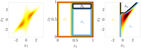
Figure 5: Truncation of a proposal $q(x_{1:2})$. Numbering left to right, [1] shows the original proposal and [2] the hierarchical partitioning of $z_{1:2}$ imposed by the tree. [3] shows the partitioning implied by $q(x_{1:2})$ and the leaf nodes on the target space $x_{1:2}$, where we note that the partition between $A_{3}$ and $A_{4}$ is nonlinear. It further shows the proposal truncated to $A_{4}$ and renormalized.

In general, $g$ can be thought of as an inverse cumulative distribution function. Namely, if we presume that $x$ is also $T$ dimensional and our proposal factorizes as

$$q(x_{1:T})=q(x_{1})q(x_{2}|x_{1})\dots q(x_{T}|x_{1:T-1})$$

then $z_{t}$ is defined by the series of cumulative distribution mappings

$$z_{t}:=\eta_{t}(x_{t};x_{1:t-1})=\int_{-\infty}^{x_{t}}q_{t}(x_{t}^{\prime}|x_{1:t-1})dx_{t}^{\prime},$$ (13)

which in turn implicitly defines $g$. As we are free to choose the form of the proposal, we can always ensure that $g$ can be calculated. In some scenarios, it might even be helpful to define $q(x)$ implicitly through $g$. Note that (13) further implies that the marginal proposals can be expressed in the form

$$q_{t}(x_{1:t})=g_{t}(z_{1:t}).$$

such that we can can sequentially generate $x_{1:T}$, as required in the SMC setting.

Another important point of interest is that it is perfectly permissible for $g$ to map multiple different $z_{1:T}$ to the same $x$. For example, this is necessary when $x$ is discrete. In this scenario, the $A_{j}$ may no longer be disjoint, but here we can instead rely on the law of the unconscious statistician: we can think in terms of performing inference on $z_{1:T}$ (for which the partitions are disjoint) and then taking the pushforward distribution this induces on $x$. Note that this does not require any algorithmic changes.

Because the distribution over $z_{1:T}$ is a uniform hypercube, the probability of generating an $x$ whose pre-image is in $B_{j}$ is just the hypervolume of $B_{j}$ (which is in turn given by the product of the lengths of $\zeta^{j}_{t}$). Therefore, after drawing from the truncated proposal $q(x|x\in A_{j})$ by sampling $\hat{z}_{1:T,j}^{n}\sim\textsc{Uniform}(B_{j})$ and setting $\hat{x}_{j}^{n}=g(\hat{z}_{1:T,j}^{n})$, we can evaluate the corresponding weights using

$$w_{j}^{n}:=\frac{\pi(\hat{x}_{j}^{n})}{q(\hat{x}_{j}^{n}|\hat{x}_{j}^{n}\in A_{j})}=\frac{\pi(\hat{x}_{j}^{n})}{q(\hat{x}_{j}^{n}|\hat{z}_{1:T,j}^{n}\in B_{j})}=\frac{\pi(\hat{x}_{j}^{n})}{q(\hat{x}_{j}^{n})}\lVert B_{j}\rVert$$ (14)

where $\lVert B_{j}\rVert$ is just the (known) area of $B_{j}$.

We finish our discussion of partitions the target space by noting that it should be possible to also adapt proposals within individual regions, in addition to the adaptation already provided by inference trees. This can be done by sampling $z_{1:T}|B_{j}$ from a non-uniform distribution which is learned adaptively, and adjusting (14) accordingly.

Appendix B Theoretical Justification

In this section, we demonstrate the correctness of the IT algorithm.

We first demonstrate that for any partitioning $\{A_{i}\}_{i\in\mathcal{I}}$ and set of consistent estimators for each partition, then the combination strategies given in §4 similarly lead to consistent estimators. Moreover, we demonstrate that this convergence holds when we combine multiple sets of estimators, each with their own partitioning, for example the parent estimator and children estimator in (5). At a high-level we make three assumptions: each constituent estimator is consistent in isolation, each set of estimators only has finite combination weight in the limit of large overall computational budget if each of constituent region estimators receives a finite proportion of that overall computational budget, and the number of each regions is finite for each estimator set. For exposition, we will, for now, assume that the $A_{i}$ are disjoint (in Assumption 1), but we show in Appendix B.1 how that this assumption can be relaxed to any proposal constructed from the form given in Appendix A.

Assumption 1.

Let $\mathbb{X}$ denote the support of $x$. For every independent estimator set $\ell\in\{1,\dots,L\}$, we are given a) a disjoint partitioning $\{A_{\ell,i}\}_{i\in\mathcal{I}_{\ell}}$ of the $\mathbb{X}$ such that $A_{\ell,i}\cap A_{\ell,j}=\emptyset$ for $i\neq j$ and $\bigcup_{i\in\mathcal{I}_{\ell}}A_{\ell,i}=\mathbb{X}$, and b) a family $\{\hat{\gamma}^{N_{\ell,i}}_{\ell,i}\}_{i\in\mathcal{I}_{\ell}}$ of estimated measures on $\mathbb{X}$

$$\hat{\gamma}^{N_{\ell,i}}_{\ell,i}\left(\cdot\right):=\frac{1}{N_{\ell,i}}\sum_{n=1}^{N_{\ell,i}}w^{n}_{\ell,i}\,\delta_{\hat{x}_{\ell,i}^{n}}\left(\cdot\right)$$

for some random variables $w^{n}_{\ell,i}$ and $\hat{x}_{\ell,i}^{n}$ such that each $\hat{\gamma}^{N_{\ell,i}}_{\ell,i}(\cdot)$ converges weakly to the following measure on $\mathbb{X}$ as $N_{\ell,i}\rightarrow\infty$

$$\gamma(x)\mathbb{I}(x\in A_{\ell,i}).$$

Further each marginal probability estimate converges in probability as follows

$$\hat{\omega}^{N_{\ell,i}}_{\ell,i}:=\frac{1}{N_{\ell,i}}\sum_{n=1}^{N_{\ell,i}}w^{n}_{\ell,i}\overset{p}{\to}\int_{\mathbb{X}}\mathbb{I}(x\in A_{\ell,i})\gamma(dx).$$

Assumption 2.

Let $k_{\ell}:{}_{\geq 0}\to{}_{\geq 0}$ be combination weight functions which produce unnormalized combination weights $k_{\ell}\left(N_{\ell}\right)$ when provided with the total number of samples used for the corresponding estimator set $N_{\ell}=\sum_{i\in\mathcal{I}_{\ell}}N_{\ell,i}$ such that $\lim_{N_{\ell}\to\infty}k_{\ell}(N_{\ell})=\infty$ for each $\ell$, each $k_{\ell}(N_{\ell})$ is finite for any finite $N_{\ell}$, and $\sum_{\ell=1}^{L}k_{\ell}(N_{\ell})>0$ whenever $R=\sum_{\ell=1}^{L}N_{\ell}>0$. We further assume that for each estimator set $\ell$, either all of the $N_{\ell,i}$ tend to infinity or none of them. More precisely, we assume there is a non-empty subset $\mathcal{L}_{0}\subseteq\{1,\ldots,L\}$ such that for all $\ell\in\mathcal{L}_{0}$ and $i\in\mathcal{I}_{\ell}$,

$$\lim\limits_{R\to\infty}N_{\ell,i}=\infty$$

and for all $\ell\not\in\mathcal{L}_{0}$,

$$\lim\limits_{R\to\infty}N_{\ell}<\infty$$

almost surely.

Assumption 3.

Each $\mathcal{I}_{\ell}$ is a finite set.

The last of these assumptions can probably be relaxed to $\mathcal{I}_{\ell}$ being a countable set, but as it will be algorithmically beneficial to ensure that the depth of the tree remains bounded, this case is of little interest anyway. The need for the second assumption is to ensure that any individual estimator which only has finite computational budget in the limit of large overall budget is given zero weight after normalization.

We are now ready to demonstrate the consistency of our estimator combination.

Lemma 1.

If Assumptions 1, 2 and 3 hold, then

$$\hat{\gamma}^{\{N_{\ell,i}\}_{\ell,i}}:=\frac{1}{\sum_{\ell=1}^{L}k_{\ell}\left(N_{\ell}\right)}\sum_{\ell=1}^{L}k_{\ell}\left(N_{\ell}\right)\sum_{i\in\mathcal{I}_{\ell}}\hat{\gamma}^{N_{\ell,i}}_{\ell,i}$$ (15)

converges weakly to the measure $\gamma(x)$ on $\mathbb{X}$ as $R\to\infty$.

Proof.

By assumption we have that each $\hat{\gamma}^{N_{\ell,i}}_{\ell,i}$ converges weakly to the measure $\gamma(x)\mathbb{I}(x\in A_{\ell,i})$ as $N_{\ell,i}$ tends to $\infty$. Thus, for each $\ell\in\mathcal{L}_{0}$, $\sum_{i\in\mathcal{I}_{\ell}}\hat{\gamma}_{\ell,i}^{N_{\ell,i}}$ converges weakly to the measure

$$\sum_{i\in\mathcal{I}_{\ell}}\gamma(x)\mathbb{I}(x\in A_{\ell,i})=\gamma(x)\sum_{i\in\mathcal{I}_{\ell}}\mathbb{I}(x\in A_{\ell,i})=\gamma(x)$$

as $R\to\infty$. The estimates for $\ell\notin\mathcal{L}_{0}$ need not converge but do not affect the final estimate as

$$\lim\limits_{R\to\infty}\frac{k_{\ell}(N_{\ell})}{\sum_{\ell=1}^{L}k_{\ell}(N_{\ell})}=0\quad\forall\ell\notin\mathcal{L}_{0}.$$

To show the claim of this theorem, we now consider an arbitrary bounded continuous function $f:\mathbb{X}\to\real$ for which we have

$$\int f(x)\,\hat{\gamma}^{\{N_{\ell,i}\}_{\ell,i}}(dx) =\int f(x)\frac{1}{\sum_{\ell=1}^{L}k_{\ell}\left(N_{\ell}\right)}\sum_{\ell=1}^{L}k_{\ell}\left(N_{\ell}\right)\sum_{i\in\mathcal{I}_{\ell}}\hat{\gamma}^{N_{\ell,i}}_{\ell,i}(dx)$$

$$=\frac{1}{\sum_{\ell=1}^{L}k_{\ell}\left(N_{\ell}\right)}\sum_{\ell=1}^{L}k_{\ell}\left(N_{\ell}\right)\sum_{i\in\mathcal{I}_{\ell}}\int f(x)\hat{\gamma}^{N_{\ell,i}}_{\ell,i}(dx)$$

which using Assumptions 1 and 2 converges as $R\to\infty$ to

$$\frac{\sum_{\ell\in\mathcal{L}_{0}}k_{\ell}\left(N_{\ell}\right)\sum_{i\in\mathcal{I}_{\ell}}\int f(x)\mathbb{I}(x\in A_{\ell,i})\,\gamma(dx)}{\sum_{\ell\in\mathcal{L}_{0}}k_{\ell}\left(N_{\ell}\right)} =\frac{1}{\sum_{\ell\in\mathcal{L}_{0}}k_{\ell}\left(N_{\ell}\right)}\sum_{\ell\in\mathcal{L}_{0}}k_{\ell}\left(N_{\ell}\right)\int f(x)\,\gamma(dx)$$

$$=\int f(x)\,\gamma(dx)$$

and thus the expectation taken with respect to $\hat{\gamma}^{\{N_{\ell,i}\}_{\ell,i}}$ converges to the true expectation $\int f(x)\,\gamma(dx)$. Now as this holds for an arbitrary $f$, this implies weak convergence as required. ∎

Corollary 1.

Let

$$\hat{\omega}^{\{N_{\ell,i}\}_{\ell,i}}:=\frac{1}{\sum_{\ell=1}^{L}k_{\ell}\left(N_{\ell}\right)}\sum_{\ell=1}^{L}k_{\ell}\left(N_{\ell}\right)\sum_{i\in\mathcal{I}_{\ell}}\hat{\omega}^{N_{\ell,i}}_{\ell,i}.$$ (16)

If the assumptions of Lemma 1 hold, then

$$\hat{\omega}^{\{N_{\ell,i}\}_{\ell,i}}\overset{p}{\to}\omega.$$ (17)

and

$$\hat{\pi}^{\{N_{\ell,i}\}}_{\ell,i}:=\frac{\hat{\gamma}^{\{N_{\ell,i}\}_{\ell,i}}}{\hat{\omega}^{\{N_{\ell,i}\}_{\ell,i}}}$$ (18)

converges weakly to the measure $\pi(x)$ on $\mathbb{X}$ as $R\to\infty$.

Proof.

Using the same arguments as Lemma 1 with $f(x)=1$ gives

$$\hat{\omega}^{\{N_{\ell,i}\}_{\ell,i}} \overset{p}{\to}\frac{1}{\sum_{\ell\in\mathcal{L}_{0}}k_{\ell}\left(N_{\ell}\right)}\sum_{\ell\in\mathcal{L}_{0}}k_{\ell}\left(N_{\ell}\right)\sum_{i\in\mathcal{I}_{\ell}}\int_{\mathbb{X}}\mathbb{I}(x\in A_{\ell,i})\gamma(dx)$$ (19)

$$=\frac{1}{\sum_{\ell\in\mathcal{L}_{0}}k_{\ell}\left(N_{\ell}\right)}\sum_{\ell\in\mathcal{L}_{0}}k_{\ell}\left(N_{\ell}\right)\int_{\mathbb{X}}\gamma(dx)$$ (20)

$$=\omega.$$ (21)

The second result now follows directly from Slutsky’s Theorem and Lemma 1. ∎

These results firstly convey that if we combine convergent estimators for the partitioned parts of the overall target, we get a convergent estimator for the target. Secondly, it implies that we can similarly combine a number of estimates for the target, which come from different partitionings. For example, we can combine a estimate $\hat{\gamma}(x)\mathbb{I}(x\in A_{j})$ for the trivial partition $\{A_{j}\}$ of $A_{j}$, with that given by combining $\hat{\gamma}(x)\mathbb{I}(x\in A_{\ell_{j}})$ and $\hat{\gamma}(x)\mathbb{I}(x\in A_{r_{j}})$ for the partitioned parts $A_{\ell_{j}}$ and $A_{r_{j}}$ where $A_{j}=A_{\ell_{j}}\cup A_{r_{j}}$, in a manner that preserves consistency, i.e. we can consistently combine parents estimates with their children. These results hold independently of how the $k_{\ell}$ are chosen, provided Assumption 2 holds. However, the variances of the associated estimates are likely to depend heavily on the choice of $k_{\ell}$ – we wish to place more weight on the partitionings with lower variance estimates.

A critical point is that the combination of estimators does not require any correction factor for the number of times that an estimator and a partition were “proposed” – i.e. we do not need to correct for the fact that more computational resources are provided for some estimates than others or because some partitions of the space are potentially larger than others. All such potential factors either cancel out, or are dealt with by the correct normalization of the truncated proposal. As such, any strategy on deciding the partitions or how often a partition is proposed only need satisfy the stated assumptions to ensure consistency. We are now thus ready to prove Theorem 1 from the main paper as follows, with the Theorem itself repeated for convenience.

See 1

Proof.

The proof follows using a combination of showing that Assumptions 1, 2 and 3 are satisfied and a recursive application of Lemma 1 and Corollary 1.

We start by considering $\hat{\gamma}_{j}(\cdot)$ and $\hat{\omega}_{j}$ for a node $j$ whose children are both leaf nodes. Here Assumption 3 is trivially satisfied as we have two estimates: the local parent estimate and the combined child estimate. By construction, the combination of a parent node and child node estimates satisfies the partitioning requirements of Assumption 1, while by the final assumption in the theorem, we have the required consistency of each of the child and parent node estimates in isolation. Thus Assumption 1 is also satisfied. Assumption 2 is satisfied through the assumption that each leaf node is visited infinitely often as the budget becomes arbitrarily large and the fact that, by construction, $c_{j}\to 1$ for the parent node as this happens unless the number of samples used to construct the local parent estimator also becomes infinitely large, in which case both estimates converge anyway.

Lemma 1 now tells us that $\hat{\gamma}_{j}(\cdot)\to\gamma(x)\mathbb{I}(x\in A_{j})$ and Corollary 1 tells us that $\hat{\omega}_{j}\to\int_{x\in A_{j}}\gamma(x)dx$ and $\hat{\pi}_{j}(\cdot)\to\pi(\cdot|x\in A_{j})$. We thus have the Theorem holds for leaf nodes and all nodes whose children a both leaves.

We can now recursively apply the same logic to show that the Theorem holds for all nodes in the tree. Specifically, we have that a node also converges if both its children nodes convergence, and so by induction all the nodes in the tree must converge. ∎

Remark 1.

This result can be trivially extended to convergence in probability, $\mathcal{L}^{P}$ convergence, and almost sure convergence of the expectation estimates, given the assumption that both the $\hat{\omega}_{j}$ and the corresponding unnormalized local expectation estimates

$$\hat{\varrho}_{j}:=\frac{1}{N_{j}}\sum_{n=1}^{N_{j}}w_{j}^{n}f\left(\hat{x}_{j}^{n}\right)$$

provide the required convergence. This follows by simply noting that the arguments in each proof remain equally valid for $\hat{\varrho}_{j}$ and for the different forms of convergence.

B.1 Discrete Variables

As explained in §A, our method for generating partitions means that they are not always disjoint as required by Assumption 1, most notably when $x$ is discrete. Fortunately, we can still deal with this case by noting that the required properties of Assumption 1 do hold in the space of $z_{1:T}$. This will require no algorithmic changes, but will require additional consideration in the proof. In this case we replace Assumption 1 with the following

Assumption 4.

Let $z_{1:T}\sim u(z_{1:T})$ be uniformly distributed on the unit hypercube $\mathfrak{Z}_{T}=[0,1]^{T}$ and let $x=g(z_{1:T})$ have density $q(x)$ and support $x\in\mathbb{X}$, where $q(x)$ is a valid importance sampling proposal for $\gamma(x)$ (see e.g. [29]). For every independent estimator set $\ell\in\{1,\dots,L\}$, we are given a) a partitioning $\{B_{\ell,i}\}_{i\in\mathcal{I}_{\ell}}$ of $\mathfrak{Z}_{T}$ such that $B_{\ell,i}\cap B_{\ell,j}=\emptyset$ for $i\neq j$ and $\bigcup_{i\in\mathcal{I}_{\ell}}B_{\ell,i}=\mathfrak{Z}_{T}$, and b) a family $\{\hat{\varphi}^{N_{\ell,i}}_{\ell,i}\}_{i\in\mathcal{I}_{\ell}}$ of estimated measures on $\mathfrak{Z}_{T}$ for all $N\geq 1$:

$$\hat{\varphi}^{N_{\ell,i}}_{\ell,i}\left(\cdot\right):=\frac{1}{N_{\ell,i}}\sum_{n=1}^{N_{\ell,i}}w^{n}_{\ell,i}\,\delta_{\hat{z}_{1:T,\ell,i}^{n}}\left(\cdot\right)$$

for some random variables $w^{n}_{\ell,i}$ and $\hat{z}_{1:T,\ell,i}^{n}$ such that each $\hat{\varphi}^{N_{\ell,i}}_{\ell,i}$ converges weakly to the following measure on $\mathfrak{Z}_{T}$ as $N_{\ell,i}\rightarrow\infty$

$$\frac{\gamma(g(z_{1:T}))\mathbb{I}(z_{1:T}\in B_{\ell,i})u(z_{1:T})}{q(g(z_{1:T}))}.$$

Further each marginal probability estimate converges in probability as follows

$$\hat{\omega}^{N_{\ell,i}}_{\ell,i}:=\frac{1}{N_{\ell,i}}\sum_{n=1}^{N_{\ell,i}}w^{n}_{\ell,i}\overset{p}{\to}\int_{\mathfrak{Z}_{T}}\frac{\gamma(g(z_{1:T}))\mathbb{I}(z_{1:T}\in B_{\ell,i})}{q(g(z_{1:T}))}u(dz_{1:T}).$$

Corollary 2.

Let $\hat{\gamma}^{N_{\ell,i}}_{\ell,i}$ denote the pushforward measure of $\hat{\varphi}^{N_{\ell,i}}_{\ell,i}$ (as per $\hat{\gamma}^{N_{\ell,i}}_{\ell,i}$ in Assumption 1), then if Assumptions 4, 2 and 3 hold,

$$\hat{\gamma}^{\{N_{\ell,i}\}_{\ell,i}}:=\frac{1}{\sum_{\ell=1}^{L}k_{\ell}\left(N_{\ell}\right)}\sum_{\ell=1}^{L}k_{\ell}\left(N_{\ell}\right)\sum_{i\in\mathcal{I}_{\ell}}\hat{\gamma}^{N_{\ell,i}}_{\ell,i}$$ (22)

converges weakly to the measure $\gamma(x)$ on $\mathbb{X}$ as $R\to\infty$.

Proof.

As per Lemma 1, the estimates for $\ell\notin\mathcal{L}_{0}$ need not converge but do not affect the final estimate. We again demonstrate the result by considering an arbitrary continuous function $f:\mathbb{X}\to\real$ for which we have

$$\int f(x)\,\hat{\gamma}^{\{N_{\ell,i}\}_{\ell,i}}(dx) =\int f(x)\frac{1}{\sum_{\ell=1}^{L}k_{\ell}\left(N_{\ell}\right)}\sum_{\ell=1}^{L}k_{\ell}\left(N_{\ell}\right)\sum_{i\in\mathcal{I}_{\ell}}\hat{\gamma}^{N_{\ell,i}}_{\ell,i}(dx)$$

$$=\frac{1}{\sum_{\ell=1}^{L}k_{\ell}\left(N_{\ell}\right)}\sum_{\ell=1}^{L}k_{\ell}\left(N_{\ell}\right)\sum_{i\in\mathcal{I}_{\ell}}\int f(x)\hat{\gamma}^{N_{\ell,i}}_{\ell,i}(dx)$$

$$=\frac{1}{\sum_{\ell=1}^{L}k_{\ell}\left(N_{\ell}\right)}\sum_{\ell=1}^{L}k_{\ell}\left(N_{\ell}\right)\sum_{i\in\mathcal{I}_{\ell}}\int f(g(z_{1:T}))\hat{\varphi}^{N_{\ell,i}}_{\ell,i}(dz_{1:T})$$

which using Assumptions 4 and 2 converges as $R\to\infty$ to

$$\frac{1}{\sum_{\ell\in\mathcal{L}_{0}}k_{\ell}\left(N_{\ell}\right)} \sum_{\ell\in\mathcal{L}_{0}}k_{\ell}\left(N_{\ell}\right)\sum_{i\in\mathcal{I}_{\ell}}\int\frac{f(z_{1:T})\gamma(g(z_{1:T}))\mathbb{I}(z_{1:T}\in B_{\ell,i})}{q(g(z_{1:T}))}u(dz_{1:T})$$

$$=\frac{1}{\sum_{\ell\in\mathcal{L}_{0}}k_{\ell}\left(N_{\ell}\right)}\sum_{\ell\in\mathcal{L}_{0}}k_{\ell}\left(N_{\ell}\right)\int\frac{f(z_{1:T})\gamma(g(z_{1:T}))}{q(g(z_{1:T}))}u(dz_{1:T})$$

$$=\int\frac{f(z_{1:T})\gamma(g(z_{1:T}))}{q(g(z_{1:T}))}u(dz_{1:T})=\int\frac{f(x)\gamma(x)}{q(x)}q(dx)=\int f(x)\,\gamma(dx)$$

as required. ∎

Given this corollary, we can now trivially extend Theorem 1 to the setting where Assumption 4 holds instead of Assumption 1 using the same arguments.

Appendix C Setting the Child Preference Factors

The child preference factors $c_{j}$ represent a relative weight given to the estimate from the child nodes in our combined estimator. In the absence of other information, it would thus be natural to set $c_{j}=\frac{M_{j}-N_{j}}{M_{j}}$ where $M_{j}$ is the total number of traversals (including running inference at the parent) and $N_{j}$ is the number of times inference has been run at the parent node, such that the estimates are weighted in proportion to the number of component samples. However, we also expect the per-sample efficiency of the child estimate to be better than the parent because of the adaptation provided by the inference tree. Therefore, we want to give more preference to the child estimates. To do this, we employ the simple, but effective, heuristic of scaling the number of child traversals as follows

$$c_{j}=\frac{\lambda^{(\mathbb{E}[d_{\text{ch}}]-d_{j})}(M_{j}-N_{j})}{N_{j}+\lambda^{(\mathbb{E}[d_{\text{ch}}]-d_{j})}(M_{j}-N_{j})}$$ (23)

where $d_{j}$ is the depth of node $j$ in the tree and $\mathbb{E}[d_{\text{ch}}]$ is the average depth of the child subtrees. Here is $\lambda\in[1,\infty)$ is preference parameters and can be interpreted as how many times more efficient we expect the $d_{j+1}$-th layer to be than the $d_{j}$-th layer. We use $\lambda=1.2$ as a default. In the context of the notation of the main paper we thus have

$$c_{j}=\frac{M_{j}-N_{j}}{M_{j}}\chi_{j}\quad\text{where}\quad\chi_{j}=\frac{\lambda^{(\mathbb{E}[d_{\text{ch}}]-d_{j})}M_{j}}{N_{j}+\lambda^{(\mathbb{E}[d_{\text{ch}}]-d_{j})}(M_{j}-N_{j})}$$ (24)

is our correction factor.

Appendix D Estimates for Empirical Variance and Effective Sample Size

When calculating terms such as the effective sample size (ESS) [29], we need to take care about the fact that our traversal strategy implies additional implicit weights through the $N_{j}$ and $c_{j}$. In short, our “expected squared weight” should not be simply calculated using $\frac{1}{N_{j}}\sum_{n=1}^{N}(w_{i}^{n})^{2}$ but instead using the scheme we now introduce. Given this expected squared weight estimator, a number of useful estimators will follow naturally.

We start by introducing an alternative formulation of the combined marginal likelihood estimate of a node as follows

$$\hat{\omega}_{j} =(1-c_{j})\frac{1}{N_{j}}\sum_{n=1}^{N_{j}}w_{j}^{n}+c_{j}\left(\hat{\omega}_{\ell_{j}}+\hat{\omega}_{r_{j}}\right)=\frac{1}{M_{j}}\sum_{m=1}^{M_{j}}w_{m}k_{m}\frac{M_{j}}{N_{j(m)}}$$ (25)

where $M_{j}$ is the number of times the node has been traversed, $\{w_{m}\}_{m=1}^{M_{j}}$ is the union of all the weights from the current node and its decedents, $k_{m}$ is a child preference weight associated with sample $m$ (e.g. $(1-c_{j})$ for a sample form the current node local estimate, $c_{j}(1-c_{j})$ for a sample from the local estimate of a child if that node is an internal node, etc.), and $N_{j(m)}$ is the number of samples that have been generated locally at the node that generated sample $m$. We thus see that the true sample weights in our combined estimator are $w_{m}k_{m}M_{j}/N_{j(m)}$ and so our estimator for the squared weight is

$$\hat{\zeta}^{2}_{j}:= \frac{1}{M_{j}}\sum_{m=1}^{M_{j}}\left(w_{m}k_{m}\frac{M_{j}}{N_{j(m)}}\right)^{2}=M_{j}\sum_{m=1}^{M_{j}}\left(\frac{w_{m}k_{m}}{N_{j(m)}}\right)^{2}$$

$$= M_{j}\left((1-c_{j})^{2}\frac{1}{N_{j}^{2}}\sum_{n=1}^{N_{j}}\left(w_{j}^{n}\right)^{2}+c_{j}^{2}\left(\frac{\hat{\zeta}_{\ell_{j}}^{2}}{M_{\ell_{j}}}+\frac{\hat{\zeta}_{r_{j}}^{2}}{M_{r_{j}}}\right)\right).$$ (26)

$\hat{\zeta}_{j}^{2}/M_{j}$ can be propagated in a similar fashion to other estimates, allowing $\hat{\zeta}^{2}_{j}$ to be estimated at any node.

Given $\hat{\zeta}^{2}_{j}$, we can straightforwardly construct various useful estimators. For example, the Monte Carlo estimator for the variance of the weight produced by a given traversal is given by

$$\sigma_{j}^{2}:=\frac{M_{j}}{M_{j}-1}\left(\hat{\zeta}^{2}_{j}-\hat{\omega}^{2}_{j}\right)$$ (27)

where the first term is Bessel’s correction. The ESS, on the other hand, is

$$\text{ESS}_{j}:=\frac{M_{j}\hat{\omega}^{2}_{j}}{\hat{\zeta}^{2}_{j}}.$$ (28)

Appendix E Derivation of the Pure-Exploitation Target

For this derivation, it will be convenient to first consider the case where the children we are deciding between are both leaf nodes and that there is some arbitrary (unknown) target function $f$, such that combined child estimate (not including the parent) is given by

$$\hat{\mu}_{\text{ch}}:=\frac{1}{N_{\ell}}\sum_{n=1}^{N_{\ell}}w_{\ell}^{n}\hat{f}_{\ell}^{n}+\frac{1}{N_{r}}\sum_{n=1}^{N_{r}}w_{r}^{n}\hat{f}_{r}^{n}$$ (29)

where $\hat{f}_{i}^{n}:=f(\hat{x}_{i}^{n})$. Now the mean squared error (MSE) of our estimator decomposes in the standard manner

$$\mathbb{E}[(\hat{\mu}_{\text{ch}}-\mu_{j})^{2}]=\operatorname*{Var}[\hat{\mu}_{\text{ch}}]+(\mathbb{E}[(\hat{\mu}_{\text{ch}}-\mu_{j})])^{2}$$

where the second term is the biased squared and all terms are implicitly conditioned on $N_{\ell}$ and $N_{r}$. Though the finite sample bias of our estimator is difficult to assert, we know that it vanishes as $N_{\ell},N_{r}\to\infty$ and, due to the central limit theorem, we can safely assume this happens faster than the standard deviation vanishes. Thus asymptotically, we only need to consider the variance to minimize the MSE. Now, invoking the conditional independence given $N_{\ell}$ and $N_{r}$ of each child estimator and each sample within those estimators, we have

$$\operatorname*{Var}[\hat{\mu}_{\text{ch}}] =\operatorname*{Var}\left[\frac{1}{N_{\ell}}\sum_{n=1}^{N_{\ell}}w_{\ell}^{n}\hat{f}_{\ell}^{n}\right]+\operatorname*{Var}\left[\frac{1}{N_{r}}\sum_{n=1}^{N_{r}}w_{r}^{n}\hat{f}_{r}^{n}\right]$$

$$=\frac{1}{N_{\ell}}\operatorname*{Var}\left[w_{\ell}^{1}\hat{f}_{\ell}^{1}\right]+\frac{1}{N_{r}}\operatorname*{Var}\left[w_{\ell}^{1}\hat{f}_{\ell}^{1}\right].$$

Using the stratified sampling results of, for example, [12], it is straightforward to show that the subsequent optimal strategy is to set

$$N_{\ell}\propto\sqrt{\operatorname*{Var}\left[w_{\ell}^{1}\hat{f}_{\ell}^{1}\right]}\quad\text{and}\quad N_{r}\propto\sqrt{\operatorname*{Var}\left[w_{r}^{1}\hat{f}_{r}^{1}\right]}.$$

Now assuming that the weights and evaluations are independent (remembering that we are considering an arbitrary $f$) we have

$$\operatorname*{Var}\left[w_{\ell}^{1}\hat{f}_{\ell}^{1}\right] =\mathbb{E}\left[\left(\hat{f}_{\ell}^{1}\right)^{2}\right]\mathbb{E}\left[\left(w_{\ell}^{1}\right)^{2}\right]-\left(\mathbb{E}\left[\hat{f}_{\ell}^{1}\right]\right)^{2}\left(\mathbb{E}\left[w_{\ell}^{1}\right]\right)^{2}$$

$$=\mathbb{E}\left[\left(\hat{f}_{\ell}^{1}\right)^{2}\right]\operatorname*{Var}\left[w_{\ell}^{1}\right]+\operatorname*{Var}\left[\hat{f}_{\ell}^{1}\right]\left(\mathbb{E}\left[w_{\ell}^{1}\right]\right)^{2}$$

$$=\operatorname*{Var}\left[\hat{f}_{\ell}^{1}\right]\left(\operatorname*{Var}\left[w_{\ell}^{1}\right]\left(1+\frac{\left(\mathbb{E}\left[\hat{f}_{\ell}^{1}\right]\right)^{2}}{\operatorname*{Var}\left[\hat{f}_{\ell}^{1}\right]}\right)+\left(\mathbb{E}\left[w_{\ell}^{1}\right]\right)^{2}\right)$$

and similarly for $\operatorname*{Var}\left[w_{r}^{1}\hat{f}_{r}^{1}\right]$. We thus have that the optimal strategy is to set (using $\sigma$ to denote standard deviation)

$$\begin{split}N_{\ell}\propto\frac{\sigma\left[\hat{f}_{\ell}^{1}\right]}{\sigma\left[\hat{f}_{\ell}^{1}\right]+\sigma\left[\hat{f}_{r}^{1}\right]}\sqrt{\left(\operatorname*{Var}\left[w_{\ell}^{1}\right]\left(1+\frac{\left(\mathbb{E}\left[\hat{f}_{\ell}^{1}\right]\right)^{2}}{\operatorname*{Var}\left[\hat{f}_{\ell}^{1}\right]}\right)+\left(\mathbb{E}\left[w_{\ell}^{1}\right]\right)^{2}\right)}\end{split}.$$ (30)

Here the first term depends only on the unknown target function. Though one might want to potentially postulate a particular dependence of $\sigma\left[\hat{f}_{\ell}^{1}\right]$ on the relative volume of the nodes, we will just presume the ratio is unknown and conservatively set it to $1$, falling in line with standard approaches for Bayesian inference where we aim to sample in proportion to the posterior, rather than artificially producing more samples in larger areas of the space to account for the potential of higher variation in the target function.

The second term depends only on statistics of the sample weights and the ratio $\left(\mathbb{E}\left[\hat{f}_{\ell}^{1}\right]\right)^{2}/\operatorname*{Var}\left[\hat{f}_{\ell}^{1}\right]$. As $f$ is unknown, we also do not know this ratio. However, we do know it must vary between $0$ (when $\mathbb{E}\left[\hat{f}_{\ell}^{1}\right]=0$ or $\operatorname*{Var}\left[\hat{f}_{\ell}^{1}\right]\rightarrow\infty$) and $\infty$ (when $\operatorname*{Var}\left[\hat{f}_{\ell}^{1}\right]=0$, i.e. the function is flat). These two respective extremes give

$$N_{\ell}\propto\sqrt{\left(\operatorname*{Var}\left[w_{\ell}^{1}\right]+\left(\mathbb{E}\left[w_{\ell}^{1}\right]\right)^{2}\right)}=\sqrt{\mathbb{E}[\left(w_{\ell}^{1}\right)^{2}]}\quad\text{and}\quad N_{\ell}\propto\sigma[w_{\ell}^{1}].$$

The latter of these corresponds to the optimal strategy for estimating the marginal likelihood, as would be expected from considering the stratified sampling results of [12] applied to estimating $\mathbb{E}[w]$. However, this strategy gives no consideration of the need to produce samples from areas of high posterior density to capture possible variations in the target function and so is highly inappropriate. Assuming the former extreme is more conservative and spends time sampling in regions of high probability mass and also those of high weight uncertainty.

Rather than taking a particular extreme, we treat

$$\kappa:=\frac{\left(\mathbb{E}\left[\hat{f}_{\ell}^{1}\right]\right)^{2}}{\operatorname*{Var}\left[\hat{f}_{\ell}^{1}\right]},\quad\kappa\in[0,\infty]$$

explicitly as a parameter of the traversal algorithm, where higher values of $\kappa$ give more emphasis to estimating the marginal likelihood and to accurate prediction of expectations of smoothly varying functions, while lower values of $\kappa$ give more emphasis to sampling regions in proportion to their marginal probabilities. We note the interesting, and perhaps counter-intuitive, result that even when $\kappa$ is its minimum possible value, the optimal traversal strategy is still not to sample in proportion to marginal probability, except in the special case where the variance of the weights is zero.

Thus far we have omitted the fact that we eventually want a normalized estimator. We deal with the former by noting that we intend to separately propagate the unnormalized estimate and the marginal likelihood estimate. Thus, except at the root node, our aim is to propagate low variance estimates of both, rather than simply low variance estimates of the ratio. Though we do not do further analysis to assess this, we choose by default to set $\kappa=1$, to reflect the fact that we thus always explicitly care about the marginal likelihood estimate.

We have also thus far omitted the fact that we need to calculate traversal strategies when the children are not leaves. Here we can use the same analysis but need to replace $\mathbb{E}\left[w_{\ell}^{1}\right]$ and $\operatorname*{Var}\left[w_{\ell}^{1}\right]$ with appropriate combined estimators. For the former, we can simply use $\hat{\omega}_{\ell}$. For the latter, we need a notion of a “single-traversal” variance in the marginal likelihood estimate. Such a metric was derived as $\hat{\sigma}_{\ell}^{2}$ in Appendix D. We thus arrive at our derivation of the unnormalized exploitation reward of node $\ell$ as

$$\hat{\tau}_{\ell}:=\sqrt{\hat{\omega}_{\ell}^{2}+(1+\kappa)\hat{\sigma}_{\ell}^{2}}.$$ (31)

Appendix F Additional Density Estimation Details

F.1 Additional Heuristics

Even though we cannot calculate it, we know that there is maximum possible log weight for each node, namely

$$\log w_{j}^{*}=\max_{z_{1:T}\in B_{j}}\log\gamma(g(z_{1:T}))+\log\lVert B_{j}\rVert-\log q(g(z_{1:T})).$$

Consequently, our density estimator (which is defined on the full real line) will typically slightly overestimate the probability of a sampling falling above the threshold. In particular, if there is a large number of samples at the node and we are only using a simple density estimator for $\psi$, we may continue to except to exceed the threshold even when previous samples suggest a saturation below the threshold.

Let $\text{e}(T)$ to denote the event $\left\{\max(w_{j}^{1:T})>w_{\text{th}}\right\}$, i.e. the event that one of $T$ independent samples exceeds the threshold if we draw $T$ samples. We now have $P(\text{e}(T))=1-(1-\Psi(\log w_{\text{th}}))^{T}$. We can further condition this on the event that we have not already seen the threshold exceeded using the likelihood $P(\neg\text{e}(N_{j})|\text{e}(T))$. To define this, we introduce an additional parameter $\log w_{\text{gap}}$ and define our likelihood to condition on the fact that none of our $N_{j}$ samples fall above $\log w_{\text{th}}$ with $\Psi$ truncated at $\log w_{\text{tr}}:=\log w_{\text{th}}+\log w_{\text{gap}}$ to reflect the fact that the true log weights are bounded, giving

$$P(\neg\text{e}(N_{j})|\text{e}(T))=\left(\frac{\Psi(\log w_{tr})-\Psi(\log w_{\text{th}})}{\Psi(\log w_{tr})}\right)^{N_{j}},$$

with Bayes’ rule in turn yielding

$$P(\text{e}(T)|\neg\text{e}(N_{j}))=\frac{\left(1-(1-\Psi(\log w_{\text{th}}))^{T}\right)P(\neg\text{e}(N_{j})|\text{e}(T))}{\left(1-(1-\Psi(\log w_{\text{th}}))^{T}\right)P(\neg\text{e}(N_{j})|\text{e}(T))+(1-\Psi(\log w_{\text{th}}))^{T}}.$$ (32)

The full definition of $\hat{p}^{s}_{j}$ actually used is then given by

$$\hat{p}^{s}_{j}:=\left(1-c_{j}\right)\frac{P(\text{e}(T)|\neg\text{e}(N_{j}))}{\text{ESS}_{j}}+c_{j}\left(\hat{p}^{s}_{\ell_{j}}+\hat{p}^{s}_{r_{j}}-\hat{p}^{s}_{\ell_{j}}\hat{p}^{s}_{r_{j}}\right).$$ (33)

F.2 Additional Intuition and Parameters

At first it might seem counter intuitive to include an ESS scaling term in $\hat{p}^{s}_{j}$ as a classic failure case for the ESS as a performance metric is if there multiple modes. However, the scenario where the local estimate has a high ESS and multiple modes is expected to be rare. Instead, one will typically have a low local ESS for any node with multiple modes but it may have children with a high ESS giving it a high combined ESS estimate. In these cases, the combined significant probability estimate $\hat{p}^{s}_{j}$ should still be high if there is any descendant $i$ with a high $\hat{p}^{s}_{i}$ and a low $\text{ESS}_{i}$. Thus in practice, scaling by the ESS does not cause the high nodes in the tree to miss multiple mode cases, while providing a more reliable metric for nodes low down in the tree.

In our approach, $T$ and $\log w_{\text{gap}}$ constitute fixed parameters which we set to $1000$ and $10$ respectively as default. On the other hand, $w_{\text{th}}$ naturally needs to change as the training progresses. We make the simple choice of setting $w_{\text{th}}$ to being the highest weight generated at any node, scaled to adjust for differences $\lVert B_{j}\rVert$ makes to the weight. An unfortunate feature of this choice is that whenever the MAP estimate changes, the $\hat{p}^{s}_{j}$ for all nodes must be updated. However, the regularity that this occurs diminishes with the number of iterations, such that it, in practice, does not lead to an increasing per-iteration computational cost as the tree is run longer.

Appendix G Additional Details on Refinement Strategy

To define our entropy metric more precisely, recall that the entropy of a continuous uniform distribution $U(s_{1},s_{2})$ is

$$\textsc{Entropy}(U(s_{1},s_{2})) =-\int_{s_{1}}^{s_{2}}{q(z_{t})\log{q(z_{t})}}\,\mathrm{d}z_{t}=\ln(s_{2}-s_{1}).$$ (34)

Assume that we propose a split at a point $s\in(s_{1},s_{2})$, and that we will later go to the left of this split with a probability $P_{\ell}$ and to the right with a probability $P_{r}=1-P_{\ell}$. This splitting and the traversal strategy give rise to a proposal of a mixture of two uniform distributions that has the following density

$$q_{s}(z_{t})=\begin{cases}d_{\ell}&\text{if }z_{t}<s,\,\text{where}\,d_{\ell}=\frac{P_{\ell}}{s-s_{1}}\\ d_{r}&\text{otherwise},\,\text{where}\,d_{r}=\frac{1-P_{\ell}}{s_{2}-s}\end{cases}$$ (35)

The entropy of this proposal is:

$$\textsc{Entropy}(p_{a}) =-\int_{s_{1}}^{s}d_{\ell}\log{d_{\ell}}\,\mathrm{d}z_{t}-\int_{s}^{s_{2}}d_{r}\log{d_{r}}\,\mathrm{d}z_{t}=P_{\ell}\log\frac{1}{d_{\ell}}+P_{r}\log\frac{1}{d_{r}}\,.$$ (36)

We can now use our empirical estimates $\hat{\omega}_{\ell}=\frac{1}{N}\sum_{i=1}^{N}\mathbb{I}(z_{t,i}\in B_{\ell})w_{i}$ and similarly $\hat{\omega}_{r}=\frac{1}{N}\sum_{i=1}^{N}\mathbb{I}(x_{i}\notin B_{\ell})w_{i}$ to define our entropy metric as

$$\textsc{Entropy}(p_{s}) =\hat{P}_{\ell}\log\frac{s-s_{1}}{\hat{P}_{\ell}}+\hat{P}_{r}\log\frac{s_{2}-s}{\hat{P}_{r}}\,\quad\text{where}\quad\hat{P}_{\ell}=\frac{\hat{\omega}_{\ell}}{\hat{\omega}_{\ell}+\hat{\omega}_{r}}\quad\text{and}\quad\hat{P}_{r}=\frac{\hat{\omega}_{r}}{\hat{\omega}_{\ell}+\hat{\omega}_{r}},$$

which is trivially equivalent to the loss given in (10) up to a normalization constant. We then choose the split $s^{*}=\operatorname{arg\,min}_{s}\textsc{Entropy}(p_{s})$ where the minimization is over our randomly sampled candidate splits.

As a minor additional heuristic aimed at avoiding splits where a small but significant proportion of the tail is contained within one child, we do not in practice use $s^{*}$ directly, instead reducing the size of the child with lower probability mass by 25%.

After choosing the best split among all candidates and separating the space in to $B_{\ell}$ and $B_{r}$, we run inference restricted to $B_{\ell}$ and $B_{r}$ separately. Then we compare the empirical estimates of the marginal likelihood for each child using a t-test, which shows how likely the results are samples from two different distributions. If the p-value is small, it suggests the split is meaningful. In that case, we accept the split, creating two new child nodes and converting the current leaf node to a discriminant note. Otherwise, we discard the split and combine the samples, adding them to the estimate of the current node. When the node is revisited, new splits are suggested and the process continues in the same way.

Appendix H Additional Experimental Details

H.1 Gaussian Mixture Model

For the GMM experiment, the IT parameters were set as $\kappa=1$, $\beta=0.1$, and $c_{j}$ as per Appendix C with $\lambda$. Denoting $\rho$ as the proportion of total iterations run thus far, the annealing parameters were given schedules of $\delta(\rho)=\frac{1}{2}\left(1+\tanh\left(20\left(0.9-\rho\right)\right)\right)$ and $\alpha(\rho)=\frac{5}{8}\left(1+\tanh\left(25\left(0.95-\rho\right)\right)\right)$. We further fixed $\beta=0$ for the last 25% of the iterations to reflect the fact that, because we are carrying out inference rather than optimization, we want to spend part of our sample budget more directly exploiting the learned tree.

Our main baseline, PI-MAIS [26] is a state-of-the-art adaptive importance sampling algorithm that runs a number of independent MCMC chains targeting the joint distribution and then uses the locations of these chains to, at each iteration, construct a mixture of Gaussian proposal distribution, with each component centered on the location of one of the chains. We used $N=100$ such chains and proposed $M=15$ samples from each chain at each iteration, noting that the algorithm requires $N(M+1)$ target evaluations. We further used an random walk kernel with covariance $0.0001{I}$ for each of the MCMC chains, while each proposal component is taken as an isotropic Gaussian with covariance $0.01{I}$.

H.2 Chaotic Dynamics Model

This model comprises of an extended Kalman filter defined as

$$x_{0} \sim\,\mathcal{N}\left(0,{I}\right)$$

$$f_{t}(x_{t}|x_{t-1}) =\,A\left(x_{t-1},\theta\right)+\upsilon_{t-1},\quad\upsilon_{t-1}\sim\mathcal{N}\left(0,0.01I\right)$$

$$g_{t}(y_{t}|x_{t}) =\,Cx_{t}+\varepsilon_{t},\quad\varepsilon_{t}\sim\mathcal{N}\left(0,0.2I\right).$$

where $C$ is a known $K\times 3$ matrix. The transition function $A\left(\cdot,\theta\right)$ dictates the underlying dynamics with parameters $\theta$. We will assume that the form of $A$ is known but not the parameters. Namely, we consider the example where the dynamics correspond to the Pickover attractor defined as

$$x_{t,1}= \;\sin\left(bx_{t-1,2}\right)-\cos\left(ax_{t-1,1}\right)x_{t-1,3}$$

$$x_{t,2}= \;\sin\left(dx_{t-1,1}\right)x_{t-1,3}-\cos\left(cx_{t-1,2}\right)$$

$$x_{t,3}= \;\sin\left(x_{t-1,1}\right)$$

where $\theta=(a,b,c,d)$. We finish the model by defining the prior on each dynamics parameter to be a uniform over $[-\pi,\pi]$. A synthetic dataset $y_{1:200}$ was generated by fixing $b=-2.3$, $a=2.5$, $d=-1.5$, $c=1.25$, $K=20$, and drawing each column of $C$ from a symmetric Dirichlet distribution with concentration $0.1$.

Our main baseline method was PMMH [4], a pseudo-marginal method where one runs an MCMC sampler targeting $p(\theta|y_{1:T})$ but with the likelihood evaluation in the MH acceptance step replaced with the unbiased ML estimate produced by an SMC sweep. For this, we use isotropic random walk proposal with a covariance of $0.0004I$. For the SMC sweeps, we used 500 particles and the bootstrap proposal.

For this experiment, the same IT parameters were used as the GMM experiment, with the exception that we changed the annealing schedules to match the lower number of iterations, setting $\delta(\rho)=\frac{1}{2}\left(1+\tanh\left(4\left(0.7-\rho\right)\right)\right)$ and $\delta(\alpha)=\frac{5}{8}\left(1+\tanh\left(10\left(0.8-\rho\right)\right)\right)$.

Appendix I PMMH Sample Paths

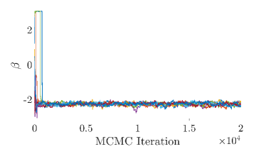
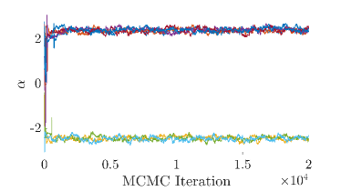
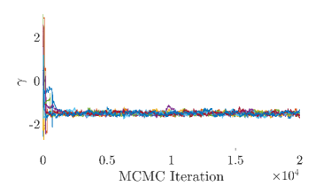
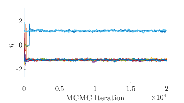
Figure 6: Sample paths of PMMH.

In the main paper, we only showed results from a single run of PMMH. To demonstrate that PMMH fails to move between modes in any of the runs, we now plot the individual sample paths as shown in Figure 6. We see that for the parameters with multiple modes, $\alpha$ and $\eta$, the PMMH sampler never moves between the modes. Thus in all runs we see PMMH was only able to pick up a single mode.

Appendix J ITs for Integration

Most adaptive sample schemes only look to approximate the posterior in the most accurate way, ignoring the fact that there might be a known function $f$ which we are trying to estimate the expectation of, namely $\mathbb{E}_{\pi(x)}\left[f(x)\right]$. Clearly, this is inferior when $f$ is known, as it ignores the fact that $f$ may have higher variability in some regions than others, such that the accuracy in those regions is more impactful on the error in the overall estimate. As well as being used as an adaptive inference algorithm, ITs are also capable of operating in this integration setting as we now demonstrate.

The integration setting for ITs varies primarily in the traversal strategy. In Section E, we indirectly showed that the optimal exploitation strategy for the known $f$ case is

$$N_{\ell}\propto\sqrt{\operatorname*{Var}\left[w_{\ell}^{1}\hat{f}_{\ell}^{1}\right]}\quad\text{and}\quad N_{r}\propto\sqrt{\operatorname*{Var}\left[w_{r}^{1}\hat{f}_{r}^{1}\right]},$$

a result that has been previously noted by, for example, [12] in the stratified sampling literature. Unlike where $f$ is unknown, $\operatorname*{Var}\left[w_{\ell}^{1}\hat{f}_{\ell}^{1}\right]$ here is a term we can directly estimate in the same way as $\sigma_{j}^{2}$ (see Section D). Defining $\hat{s}_{j}^{2}$ as the equivalent of $\hat{\sigma}_{j}^{2}$ when replacing the weights with $w_{j}^{n}\hat{f}_{j}^{n}$, this gives that exploitation target is simply

$$\tau_{j}^{\text{int}}=\hat{s}_{j}.$$ (37)

Unfortunately, our exploration strategy using density estimation does not translate so simply to the integration setting. We thus leave developing an analogous approach to future work, and simply set

$$u_{\ell_{j}}=\frac{1}{M_{\ell_{j}}}\left(\left(\frac{s_{\ell_{j}}}{s_{j}}\right)^{(1-\alpha)}+\beta\frac{\lVert B_{\ell_{j}}\rVert}{\lVert B_{j}\rVert}\frac{\log M_{j}}{\sqrt{M_{\ell_{j}}}}\right).$$ (38)

This target is now analogous to that discussed in [12] and so their regret analysis should still apply.

To demonstrate that IT are still useful in this integration setting even without a principled exploration term in the traversal target, we conducted an experiment based on a network model. Here our network

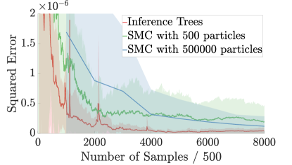
Figure 7: Convergence of ITs on network model. Solid lines show mean over 10 runs, with shaded region showing $\pm$ one standard deviation.

has weighted edges and we wish to estimate if the shortest path between two points exceeds a threshold. One possible application of such models would be in modeling a traffic network, where the edges are streets connecting two points and the weights correspond to the commuting times on different edges which are stochastic due to traffic levels and correlated because of the proximity of different streets to one another. We thus assume that there are noisy, correlated, observations for the edges weights, requiring inference, while our threshold function means we are in a “known $f$” scenario, namely we are estimating a form of tail integral.

The model is formally defined as

$$x_{1:T} \sim\mathcal{N}(x_{1:T};\mu,\Sigma)$$ (39)

$$y_{t}|x_{t} \sim\textsc{Student-T}\left(\frac{y_{t}-x_{t}}{\sigma};\nu\right)\quad\forall t\in\{1,\dots,T\}$$ (40)

where $x_{t}$ represents the unknown weights of edges, $y_{t}$ are noisy observations of those weights, and $\mu,\Sigma,\nu$, and $\sigma$ are known fixed parameters. Synthetic data was generated by setting $T=10$, $\mu=[3,\dots,3]$, $\Sigma=I$, $\sigma=0.1$, and $\nu=5$. We take the threshold as $3.8$ and look to estimate the probability that the shortest path exceeds this threshold, which in our traffic analogy would correspond to not being able to reach a destination on time. We used SMC as the base inference with $500$ particles and used batches of $8$ runs as per the chaos example. Figure 7 shows that IT outperform both SMC with the same number of samples and SMC with $1000$ times more samples.

References

- Agrawal and Goyal [2012] S. Agrawal and N. Goyal. Analysis of Thompson sampling for the multi-armed bandit problem. In Conference on Learning Theory, pages 39–1, 2012.
- Andrieu and Roberts [2009] C. Andrieu and G. O. Roberts. The Pseudo-marginal Approach for Efficient Monte Carlo Computations. The Annals of Statistics, pages 697–725, 2009.
- Andrieu and Thoms [2008] C. Andrieu and J. Thoms. A tutorial on adaptive MCMC. Statistics and computing, 18(4):343–373, 2008.
- Andrieu et al. [2010] C. Andrieu, A. Doucet, and R. Holenstein. Particle Markov chain Monte Carlo methods. Journal of the Royal Statistical Society: Series B (Statistical Methodology), 72(3):269–342, 2010.
- Auer et al. [2002] P. Auer, N. Cesa-Bianchi, and P. Fischer. Finite-time Analysis of the Multiarmed Bandit Problem. Machine learning, 47(2-3):235–256, 2002.
- Bérard et al. [2014] J. Bérard, P. Del Moral, A. Doucet, et al. A lognormal central limit theorem for particle approximations of normalizing constants. Electronic Journal of Probability, 19, 2014.
- Berry and Fristedt [1985] D. A. Berry and B. Fristedt. Bandit problems: sequential allocation of experiments (monographs on statistics and applied probability). London: Chapman and Hall, 5:71–87, 1985.
- Browne et al. [2012] C. B. Browne, E. Powley, D. Whitehouse, S. M. Lucas, P. I. Cowling, P. Rohlfshagen, S. Tavener, D. Perez, S. Samothrakis, and S. Colton. A Survey of Monte Carlo Tree Search Methods. IEEE Transactions on Computational Intelligence and AI in games, 4(1):1–43, 2012.
- Bugallo et al. [2017] M. F. Bugallo, V. Elvira, L. Martino, D. Luengo, J. Miguez, and P. M. Djuric. Adaptive importance sampling: the past, the present, and the future. IEEE Signal Processing Magazine, 34(4):60–79, 2017.
- Cappé et al. [2004] O. Cappé, A. Guillin, J.-M. Marin, and C. P. Robert. Population Monte Carlo. Journal of Computational and Graphical Statistics, 13(4):907–929, 2004.
- Cappé et al. [2008] O. Cappé, R. Douc, A. Guillin, J.-M. Marin, and C. P. Robert. Adaptive Importance Sampling in General Mixture Classes. Statistics and Computing, 18(4):447–459, 2008.
- Carpentier et al. [2015] A. Carpentier, R. Munos, and A. Antos. Adaptive strategy for stratified Monte Carlo sampling. Journal of Machine Learning Research, 16:2231–2271, 2015.
- Cornebise et al. [2008] J. Cornebise, É. Moulines, and J. Olsson. Adaptive Methods for Sequential Importance Sampling with Application to State Space Models. Statistics and Computing, 18(4):461–480, 2008.
- Cornuet et al. [2012] J. Cornuet, J.-M. MARIN, A. Mira, and C. P. Robert. Adaptive Multiple Importance Sampling. Scandinavian Journal of Statistics, 39(4):798–812, 2012.
- Douc et al. [2007] R. Douc, A. Guillin, J.-M. Marin, and C. P. Robert. Convergence of Adaptive Mixtures of Importance Sampling Schemes. The Annals of Statistics, pages 420–448, 2007.
- Doucet et al. [2001] A. Doucet, N. De Freitas, and N. Gordon. An introduction to sequential Monte Carlo methods. In Sequential Monte Carlo methods in practice, pages 3–14. Springer, 2001.
- Doucet et al. [2006] A. Doucet, M. Briers, and S. Sénécal. Efficient Block Sampling Strategies for Sequential Monte Carlo Methods. Journal of Computational and Graphical Statistics, 15(3):693–711, 2006.
- Doucet et al. [2015] A. Doucet, M. Pitt, G. Deligiannidis, and R. Kohn. Efficient implementation of markov chain monte carlo when using an unbiased likelihood estimator. Biometrika, 102(2):295–313, 2015.
- Etoré and Jourdain [2010] P. Etoré and B. Jourdain. Adaptive optimal allocation in stratified sampling methods. Methodology and Computing in Applied Probability, 12(3):335–360, 2010.
- Etore et al. [2011] P. Etore, G. Fort, B. Jourdain, and E. Moulines. On adaptive stratification. Annals of operations research, 189(1):127–154, 2011.
- Gu et al. [2015] S. Gu, Z. Ghahramani, and R. E. Turner. Neural Adaptive Sequential Monte Carlo. In Advances in Neural Information Processing Systems, pages 2629–2637, 2015.
- Kawai [2010] R. Kawai. Asymptotically optimal allocation of stratified sampling with adaptive variance reduction by strata. ACM Transactions on Modeling and Computer Simulation (TOMACS), 20(2):9, 2010.
- Kocsis and Szepesvári [2006] L. Kocsis and C. Szepesvári. Bandit Based Monte-Carlo Planning. In ECML, volume 6, pages 282–293. Springer, 2006.
- Liang et al. [2011] F. Liang, C. Liu, and R. Carroll. Advanced Markov Chain Monte Carlo Methods: Learning from Past Samples, volume 714. John Wiley & Sons, 2011.
- Lin et al. [2013] M. Lin, R. Chen, J. S. Liu, et al. Lookahead Strategies for Sequential Monte Carlo. Statistical Science, 28(1):69–94, 2013.
- Martino et al. [2017] L. Martino, V. Elvira, D. Luengo, and J. Corander. Layered adaptive importance sampling. Statistics and Computing, 27(3):599–623, 2017.
- Neufeld [2016] J. Neufeld. Adaptive Monte Carlo Integration. PhD thesis, University of Alberta, 2016.
- Neufeld et al. [2014] J. Neufeld, A. Gyorgy, C. Szepesvari, and D. Schuurmans. Adaptive Monte Carlo via Bandit Allocation. In Proceedings of the 31st International Conference on Machine Learning, volume 32, pages 1944–1952, 2014.
- Owen [2013] A. B. Owen. Monte Carlo theory, methods and examples. 2013.
- Pitt et al. [2012] M. K. Pitt, R. dos Santos Silva, P. Giordani, and R. Kohn. On some properties of markov chain monte carlo simulation methods based on the particle filter. Journal of Econometrics, 171(2):134–151, 2012.
- Rainforth et al. [2016] T. Rainforth, T. A. Le, J.-W. van de Meent, M. A. Osborne, and F. Wood. Bayesian Optimization for Probabilistic Programs. In Advances in Neural Information Processing Systems, pages 280–288, 2016.
- Silver et al. [2016] D. Silver, A. Huang, C. J. Maddison, A. Guez, L. Sifre, G. Van Den Driessche, J. Schrittwieser, I. Antonoglou, V. Panneershelvam, M. Lanctot, et al. Mastering the game of go with deep neural networks and tree search. nature, 529(7587):484–489, 2016.