The Stripe 82 1-2 GHz Very Large Array Snapshot Survey: Multiwavelength Counterparts

Abstract

We have combined spectrosopic and photometric data from the Sloan Digital Sky Survey (SDSS) with $1.4$ GHz radio observations, conducted as part of the Stripe 82 $1-2$ GHz Snapshot Survey using the Karl G. Jansky Very Large Array (VLA), which covers $\sim 100$ sq degrees, to a flux limit of 88 $\muup$Jy rms. Cross-matching the $11\,768$ radio source components with optical data via visual inspection results in a final sample of $4\,795$ cross-matched objects, of which $1\,996$ have spectroscopic redshifts and $2\,799$ objects have photometric redshifts. Three previously undiscovered Giant Radio Galaxies (GRGs) were found during the cross-matching process, which would have been missed using automated techniques. For the objects with spectroscopy we separate radio-loud Active Galactic Nuclei (AGN) and star-forming galaxies (SFGs) using three diagnostics and then further divide our radio-loud AGN into the HERG and LERG populations. A control matched sample of HERGs and LERGs, matched on stellar mass, redshift and radio luminosity, reveals that the host galaxies of LERGs are redder and more concentrated than HERGs. By combining with near-infrared data, we demonstrate that LERGs also follow a tight $K-z$ relationship. These results imply the LERG population are hosted by population of massive, passively evolving early-type galaxies. We go on to show that HERGs, LERGs, QSOs and star-forming galaxies in our sample all reside in different regions of a WISE colour-colour diagram. This cross-matched sample bridges the gap between previous ‘wide but shallow’ and ‘deep but narrow’ samples and will be useful for a number of future investigations.

1 Introduction

A multi-wavelength approach to astronomy, where observations are conducted at different wavelengths and combined, is imperative to glean critical information about the astrophysical processes that occur throughout the Universe. In extragalactic studies, combining large multi-wavelength datasets can help us understand how the star formation rate (SFR) of galaxies evolves, the subsequent stellar mass ($M^{*}$) build up of the Universe and reveal the role of Active Galactic Nuclei (AGN) via feedback processes.

Traditionally the largest galaxy surveys in area have been conducted at optical wavelengths, which include the Sloan Digital Sky Survey (SDSS; York et al., 2000) and 2 Degree Field Galaxy Redshift Survey (2DFGRS; Colless et al., 2001). In the near future however, some of the largest surveys will be conducted at radio wavelengths with the arrival of the Square Kilometre Array (SKA), which will detect many hundreds of millions (if not billions) of radio sources. Currently several SKA precursor telescopes such as MeerKAT and the Australian Square Kilometre Array Pathfinder (ASKAP) array are in the process of being constructed. These will conduct a number of radio continuum surveys such as The MeerKAT International GHz Tiered Extragalactic Exploration (MIGHTEE) Survey (Jarvis et al., 2017), the MeerKAT Large Area Synoptic Survey (MeerKLASS; Santos et al., 2017) and the Evolutionary Map of the Universe (EMU; Norris et al., 2011). Furthermore, The LOw Frequency ARray (LOFAR; van Haarlem et al., 2013) is underway and producing deep radio maps at $\sim 150$ MHz (See Hardcastle et al. (2016) and Williams et al. (2016) for examples), while the Giant Metrewave Radio Telescope (GMRT) is also undergoing an upgrade to include wide-band receivers, which will eventually allow us to make deep $610$ MHz surveys (e.g. Whittam et al. 2017; Ocran et al. 2017) routinely.

For the first time, both optical and radio surveys will probe the same population of galaxies instead of being limited to the brightest galaxies (in both the radio and optical regimes). Finding the optical counterparts to these radio sources, with either pre-existing optical data or taken as follow up observations, will be of vital importance to determine their redshifts and therefore physical properties, such as their luminosities and derived quantities such as SFRs and $M^{*}$.

However, cross-matching optical and radio datasets can be troublesome for a number of reasons. Firstly, not all radio sources will be detected at optical wavelengths. Secondly, radio continuum surveys detect a number of different populations with a range of radio morphologies. While single component radio sources can easily be matched to their optical counterparts, many objects are extended and made up of several radio components including a core, lobes and jets. Identifying the components which are part of the same source and locating the optical counterpart automatically is particularly challenging. Thirdly, the relatively low resolution (synthesised beams $>5^{\prime\prime}$) of many radio surveys, combined with the high density of objects in optical surveys means that there are several potential optical counterparts for a single radio source.

A large number of the deepest current continuum surveys have used the Karl G. Janksy Very Large Array (VLA) to observe a number of classical fields. These include deep VLA observations of Elais N1 (Taylor & Jagannathan, 2016), 3 GHz observations of the Cosmic Evolution Survey (COSMOS) field (Smolčić et al., 2017), The Chandra Deep Field South (CDFS) (Padovani et al., 2011) and observations of the Visible and Infrared Survey Telescope for Astronomy (VISTA) Deep Extragalactic Observations (VIDEO) regions (Heywood et al. (In prep.)) However, there is a gap between these deep surveys and the very wide but shallow surveys, such as Faint Images of the Radio Sky at Twenty-Centimeters (FIRST, Becker et al., 1995) and NRAO VLA Sky Survey (NVSS, Condon et al., 1998) surveys. For this reason we carried out a medium-deep survey over $100$ sq degrees of the SDSS Stripe82 region (Heywood et al., 2016).

In this paper we outline our method of cross-matching this new 1.4 GHz VLA Radio Snapshot Survey with coadded optical data, covering $~{}100$ sq degrees of the SDSS Stripe 82 region. The photometric and spectroscopic observations of galaxies and quasars in this region will allow a range of science to be investigated, which we discuss. Here we show; the $K-z$ relationship of galaxies, using near-infrared data from the VICS82 survey (Geach et al., 2017) and the Wide-field Infrared Survey Explorer (WISE, Wright et al., 2010). We then go on to investigate the WISE colours of star-forming galaxies, quasars and the High and Low Excitation Radio Galaxy (HERG and LERG) subpopulations of radio-loud AGN (AGN which show an excess of radio emission compared to their optical emission).

The structure of this paper is as follows: in Section 2 we describe the radio and optical datasets we cross-match. In Section 3 we explain the process used to cross-match these datasets. In Section 4 we describe the properties of the cross-matched sample and the method we use to divide star-forming galaxies and radio-loud AGN. We highlight a number of new giant radio galaxies discovered in the cross-matching process in Section 5. In Section 6 we describe our method of separating star-forming galaxies and radio-loud AGN, and how we divide the radio-loud AGN into HERGs and LERGs. The host properties of the HERGs and LERGs are presented in Section 7. In Section 8 we determine the $K-z$ relation of radio galaxies using near-infrared data from the VICS82 survey and WISE. We show the WISE colour-colour diagram of our radio sample in Section 9. Finally we conclude and discuss the future work that will be conducted with this dataset in Section 10. Throughout this paper we assume the following cosmological constants: $H_{0}=70$ kms^−-1 Mpc^−-1, $\Omega_{m}=0.3$ and $\Omega_{\Lambda}=0.7$. Unless stated all magnitudes are AB magnitudes. A Kroupa (2001) Initial Mass Function is assumed in the determination of the stellar masses and estimates of the SFR.

2 Data

2.1 Radio Data

The primary radio dataset used here is the Heywood et al. (2016) Snapshot Survey, hereafter H16. Using the VLA in a CnB configuration, $\sim 100$ sq degrees of SDSS Stripe 82 were observed at 1-2 GHz. These consist of $1026$ snapshot pointings coincident with the Eastern and Western regions observed by the VLA in the A configuration by Hodge et al. (2011). Each pointing was observed with an integration time of 2.5 minutes. The data reduction process is fully described in H16. In brief the data reduction was initially conducted using the NRAO pipeline, which makes use of a set of CASA (McMullin et al., 2007) commands to flag bad data, to remove radio frequency interference (RFI), to calibrate the data and to combine the pointings into a mosaic. The continuum images produced have a $16\times 10$ arcsecond resolution with an effective $1\sigma$ depth of $88$ $\muup$Jy beam^-1.

After producing mosaics for the East and West regions, a source catalogue was produced using the Python Blob Detection and Source Finder (PyBDSF, Mohan & Rafferty, 2015). The resulting catalogue contains $11\,768$ radio source components detected above $5\sigma$. The East and West regions contain $5\,674$ and $6\,594$ sources respectively. Due to the use of the a hybrid CnB configuration, the survey has good sensitivity to diffuse emission from low-surface brightness structures and objects with extended radio emission, and is complementary to the previous 1.4 GHz VLA survey in the region by Hodge et al. (2011), conducted in the A-array. The excellent resolution of the Hodge et al. (2011) survey, of $1.5\arcsec$, provides the positional accuracy that is advantageous when cross-matching radio and optical data.

2.2 Optical data

The SDSS data we use is only briefly described here, for much greater detail the reader is referred to York et al. (2000) and subsequent data release papers. The SDSS is a photometric and spectroscopic survey which makes use of a dedicated 2.5-m telescope situated on Apache Point, New Mexico. Photometry in five broad-band filters, $ugriz$, is conducted using a mosaic CCD camera (Gunn et al., 1998) and calibrated with a 0.5-m telescope (Hogg et al., 2001).

In this study we use photometry and spectroscopy from Stripe 82 of the SDSS ‘Southern Survey’ (Adelman-McCarthy et al., 2006). In its entirety, Stripe 82 consists of a $275\deg^{2}$ strip across the Southern Galactic Pole (SGP) centred along the celestial equator ranging from $-50<\alpha<60\deg$ and $-1.25<\delta<1.25\deg$ and has been observed multiple (between $20$ and $40$) times. The repeated observations of the region allows deeper coadded images to be made, which are $\sim 2$ mags fainter than a single SDSS pointing, with a limit of $r\approx 23$ mag (Annis et al., 2014). In the cross-matching process we make use of the coadded images in the regions surrounding each of the sources in the H16 catalogue that are available from the SDSS Data Archive Server (DAS) and labelled as runs $106$ and $206$.

In this paper we first attempt to match the H16 radio data to spectroscopically observed galaxies and quasars if available. In Stripe 82 multiple spectroscopic campaigns have taken place which include the SDSS I-IV main galaxy samples (MGS), the Luminous Red Galaxy (LRG) sample (Eisenstein et al., 2001), and the Baryon Oscillation Spectroscopic Survey (BOSS, Dawson et al., 2013). Data from these surveys have been released as part of the SDSS DR14 (Abolfathi et al., 2017). In the region of the H16 survey there are $\sim 84\,000$ objects with spectroscopic redshifts.

If spectroscopic data is unavailable for a particular source, we attempt to match the radio sources to objects in the photometric redshift catalogue of Reis et al. (2012). These photometric redshifts made use of coadded image runs of Annis et al. (2014) and were determined using an Artificial Neural Network technique. This resulted in the redshifts of $\sim 13$ million objects classified as galaxies (type $=3$ sources in the SDSS database) with $r<24.5$.

3 Cross-Matching

Cross-matching of the radio and optical datasets was done via the visual inspection of all $11\,768$ radio sources in the Heywood et al. (2016) catalogue. Overlays are produced using the Astronomical Plotting Library in Python (APLpy, Robitaille & Bressert, 2012), consisting of radio contours of the H16 sources and corresponding Hodge et al. (2011) contours, overlayed on top of the coadded $r$-band Stripe 82 images. Positions of all objects in the spectroscopic and photometric catalogues are also plotted.

To aid in the visual classification, two overlays are made for each source, one being a ‘zoomed’ overlay of size 0$.5^{\circ}\times 0.5^{\circ}$ and a larger overlay of size $3.0^{\circ}\times 3.0^{\circ}$, both centred on the radio source. Having these two overlays allows the correct counterpart to be identified more easily when dealing with close pairs of galaxies or crowded fields. Large extended radio sources or those with widely spaced components can also be seen clearly in the larger cutouts. The Hodge et al. (2011) and H16 image contours complement each other well, as the greater resolution of the Hodge et al. (2011) survey ($\sim 1.5\arcsec$ as opposed to $\sim 15\arcsec$ for H16) allows a more stringent cross-match, while the H16 data allows extended emission to be detected.

Using a Python script we call Xmatchit, pairs of overlays can be simultaneously displayed and users are prompted to classify whether or not the radio sources correspond to optical counterparts in the spectroscopic or photometric redshift catalogues. If the object is a match, the code then prompts the user to write the match ID and then attempt to classify the radio morphology of the object as FRI, FRII, compact or unknown. The code records all this as output. If any optical matches are in both spectroscopic and photometric catalogues, they are assigned a spectroscopic redshift. The code used to make the overlays and the Xmatchit code are available at https://github.com/MattPrescottAstro/.

Despite being time consuming, subjective and difficult to test, visual inspection is acknowledged to be more reliable than the current automated methods for cross-matching optical and radio datasets (see Fan et al. 2015). It has the advantage that spurious sources caused by imaging and deconvolution errors can be readily identified. Furthermore, large extended sources such as Giant Radio Galaxies (GRGs, see Section 5) or interesting sources such as X-shaped radio sources (Cheung, 2007; Roberts et al., 2018) can be identified, which would be easily missed simply by matching upon coordinates or via automated methods such as the Likelihood Ratio technique (E.g. Smith et al. 2011; McAlpine et al. 2012).

In order to ensure we have robust cross-matches, the radio sources were divided into batches of 100 and inspected by 3 different classifiers. The Xmatchit output for each observer in each batch was then compared to find mismatches. Overlays for any mismatches between the classifiers were then re-inspected and re-classified by the $3$ different classifiers together. $740$ radio source components ($6$ per cent of the total number) were re-inspected. After the re-inspection process, all the outputs are concatenated and the H16 fluxes of objects with multiple radio components were combined to produce a final optical/radio cross-matched sample. $21$ sources appear as single component sources in the lower resolution H16 data but are resolved into two or more separate, unrelated sources in the higher resolution Hodge et al. 2011 image, each with its own separate optical counterpart. These sources are split into separate entries in the final catalogue, with one entry per optical object. For these sources the original H16 flux density of the blended sources is divided between the two (or more) separate objects, weighted so that the ratio of the fluxes of the separate objects is the same as the ratio of the source fluxes in the Hodge et al. catalogue.

Overall we find we are able to cross-match $\sim 57$ per cent ($6\,754$ out of $11\,768$) of the initial sample of radio components, to $4\,795$ optical counterparts. The $6\,754$ cross-matched radio components can be broken down as $2\,971$ radio components associated with $1\,996$ optical counterparts with DR14 SDSS/BOSS spectra and $3\,783$ radio components associated with $2\,799$ optical counterparts with photometric redshifts from the Reis et al. (2012) catalogue. The percentage of radio sources that we have cross-matched to spectroscopic counterparts ($17$ per cent, $1\,996/11\,768$) is an improvement over many previous samples covering large areas. For example Prescott et al. (2016) found that around $10$ per cent of radio source components from a $325$ MHz GMRT radio survey of the GAMA fields could be cross-matched to a spectroscopic counterpart. Sadler et al. (2002) and Mauch & Sadler (2007) found that $\sim 1$–$2$ per cent of NVSS radio source components are detected in the 2dFGRS and 6 degree Field Galaxy Survey (6dFGS Jones et al., 2004).

The numbers of radio components that can be matched to single optical counterpart (either photometric or spectroscopic object) can be seen in Figure 1. This shows the $3\,738$ objects are comprised of a single radio component and $1\,057$ objects are made up of mulitple radio components. The mean number of radio components per optical counterpart is $1.4$. Examples of several cross-matches with different radio morphologies that are included in the sample can be seen in Figure 2.

Figure 1: Histogram of the number of H16 radio components belonging to a single optical object. The majority of cross-matched counterparts have a single radio component.

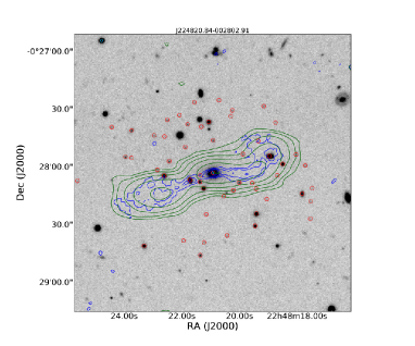
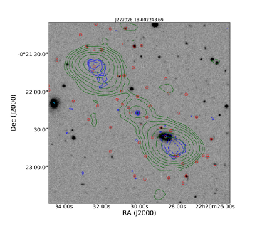
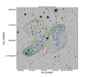
Figure 2: Examples of cross-matched sources in our catalogue; the upper left panel reveals a radio galaxy with an FRI morphology. The upper right panel shows an FRII radio galaxy. The middle left panel displays a nearby star-forming galaxy. The middle right panel shows a compact radio source which is produced by a QSO at $z=4.65$. The lower panel shows an x-shaped radio source belonging to a ‘Green Bean’ galaxy at $z=0.28$ (Schirmer et al., 2013), highlighting the extended diffuse radio emission the H16 observations detect. 1.4 GHz radio contours of the H16 survey can be seen in green, which is complimentary to the Hodge et al. (2011) data seen in blue. These are overlayed on top of optical Stripe 82 SDSS $r$-band images. Objects with spectra from SDSS DR14 surveys are indicated with cyan circles. Objects in the photometric catalogues of Reis et al. (2012) can be seen as red circles. Cutout sizes for the four upper panels are $2.5\arcmin\times 2.5\arcmin$. For the lower panel the cutout size is $4\arcmin\times 4\arcmin$.

3.1 Positional Offsets

The positional offsets between the optical and radio coordinates for the single component radio sources matched to the spectroscopic and photometric catalogues can be seen in Figure 3.

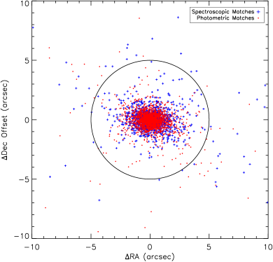
Figure 3: The positional offsets between the radio and optical coordinates for each of single component radio sources in the cross-matched catalogue. The solid black circle indicates a radius of $5\arcsec$. The mean offset between cross-matches is $0.79\arcsec$ for the spectroscopic sample (blue crosses) and $0.76\arcsec$ for the photometric sample (red dots).

In a similar way to Prescott et al. (2016), we test our matching process by measuring the positional offsets between SDSS sources in the input spectroscopic catalogue, and the nearest radio source component in the H16 catalogue. This is then compared to the mean positional offsets found between $10$ iterations of the optical catalogue with randomised positions and the nearest radio source component. We repeat this same process to check our cross-matching with the SDSS objects in photometric redshift catalogue. Here we want to determine how many single radio components we expect to match so we remove radio components that are within $3$′of each other. This leaves a sample of $5\,037$ ‘isolated’ radio source components from the initial $11\,768$ radio source components in the H16 catalogue.

Figure 4 shows the distribution of the nearest matches between $83\,742$ SDSS objects in our spectroscopic sample and the $5\,037$ radio sources, in the combined East and West regions of Stripe 82 that the radio survey covers, as well as the mean of $10$ optical catalogues with randomised positions and the radio sources. The corresponding plot for the photometric catalogue can be seen in Figure 5. This photometric catalogue contains $6\,242\,226$ objects covering our Stripe 82 regions.

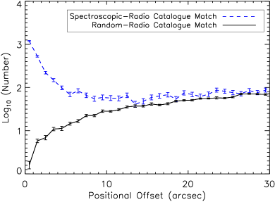
Figure 4: Positional offsets between each of the $83\,742$ SDSS objects with spectroscopic redshifts, matched to the nearest of the $5\,037$ radio source components that are isolated within $3\arcmin$ of each other (blue dashed line). This is compared to the positional offsets between the mean of $10$ random SDSS catalogues matched to the nearest isolated radio source (black solid line) component.

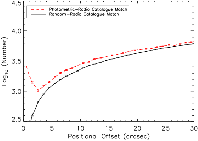
Figure 5: Positional offsets between each of the $6\,242\,226$ SDSS objects with photometric redshifts, matched to the nearest of the $5\,037$ radio source components that are isolated within $3\arcmin$ (red dashed line). This is compared to the positional offsets between the mean of $10$ random SDSS catalogues matched to the nearest isolated radio source component (black solid line).

Both of these figures show a clear excess at small radii, which can be attributed to there being true matches between the datasets. As in Best et al. (2005a), an excess of matches between the real optical/radio catalogue can be seen out to large radii in Figures 4 and 5. This is because galaxies in the optical catalogue are clustered, which means that on average there are more galaxies within $3\arcmin$ of a galaxy in the real catalogue than there are within the same distance of a random position in the sky. As some of these galaxies will host radio sources, there is therefore an increased chance of there being a radio source within $3\arcmin$ of a galaxy in the real optical catalogue than within $3\arcmin$ of a random position, resulting in the excess of matches seen Figures 4 and 5.

For the spectroscopic catalogue match, the real and random matches converge around an offset of $~{}10\arcsec$. Integrating the numbers of matches under the curves out to an offset of $10\arcsec$ yields $1\,353$ matches between the real optical/radio catalogues and $65$ matches between the random/radio catalogue which indicates we should expect to find $1\,288$ radio component radio sources with a counterpart in the spectroscopic catalogue. This is entirely consistent with our final sample of $1\,516$ single component radio sources which have spectroscopic counterparts, considering some of extended radio sources have a separation $>10\arcsec$ between one or more of the radio components (e.g. hot-spots) and the spectrocopic counterpart. For the photometric catalogue, the curves converge at around $5\arcsec$, and integration out to this radius yields $3\,909$ real optical/radio matches and $1\,447$ random optical/radio matches, meaning we should find $2\,462$ radio sources which have optical matches and photometric redshifts. This too is consistent with our final sample of $2\,222$ single component radio sources having a counterpart with a photometric redshift, as some of the optical counterparts have both photometric and spectroscopic redshifts, and any cross-match to these is assigned to the spectroscopic sample. The difference in where the curves converge ($5\arcsec$ for the photometric sample and $10\arcsec$ for the spectroscopic sample) is because the sources in the spectroscopic sample are at lower redshifts than those in the photometric sample, which means that they generally have larger angular sizes. This results in larger separations between the radio components (often the lobes of radio galaxies) and their optical counterpart (which is coincident with the core) for the sources in the spectroscopic catalogue than for those in the photometric catalogue, which are generally at higher redshifts.

3.2 Photometric Redshifts

The accuracy of the photometic redshifts used in this paper are discussed in detail in Reis et al. (2012). For our radio cross-matched sample the accuracy of the photometric redshifts can be estimated by comparing matches that have both spectroscopic ($z_{sp}$) and photometric redshift ($z_{ph}$) measurements. In Figure 6 we compare $z_{sp}$ and $z_{ph}$ for $1\,445$ galaxies (type = $3$ sources) which have reliable spectroscopic redshifts ($zwarning=0$). The spread in the between that redshift estimates can be defined as $\Delta z/(1+z_{sp})$ where $\Delta z=z_{sp}-z_{ph}$. Following Ilbert et al. (2006) and Jarvis et al. (2013), we determine the normalized median absolute deviation (NMAD) in this spread to find that ${\rm NMAD}=0.022$ i.e. the values are in good agreement with each other. Defining outliers as those with $|z_{sp}-z_{ph}|/(1+z_{sp})>0.15$, we find that only $19$ galaxies or $1.3$ per cent of the this sample have poorly determined photometric redshifts. This means that we can be reasonably confident of the accuracy of the redshift estimates for the remainder of the sample for which no spectroscopic redshifts are available.

Figure 6: Comparison between the spectroscopic and photometric redshifts of $1\,445$ galaxies in our sample. The black solid line indicates where the two values are equal.

4 Sample Properties

The sky coverage of our cross-matched samples in the Western and Eastern regions of Stripe 82 can be seen in Figure 7, showing the positions of objects with photometric redshifts as red points, along with spectroscopically observed galaxies and quasars (‘QSOs’), as blue crosses and green crosses respectively. Here the ‘QSO’ and ‘galaxy’ classifications used are SDSS spectroscopic classifications taken from the SpecObj catalogue, with the sample being made up of $415$ QSOs and $1581$ galaxies. The noticeable gap in the Western region of Figure 7 is due to a lack of radio data, caused by unobserved scheduling blocks at the VLA.

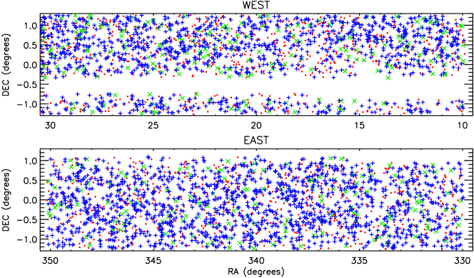
Figure 7: Coordinates of the cross matches in the East and West fields within Stripe 82. Red points indicate the objects with photometric redshifts. Galaxies with SDSS spectra can be seen as blue plus symbols and QSOs as green crosses. The gap in the western field of Stripe 82 is due to a lack of radio observations.

In Figure 8 we show the redshift distributions of our cross-matched sample. The photometric sample covers $0.0<z<1.5$, with a median redshift of $z=0.78$. Galaxies with spectroscopic redshifts are observed over the range $0.0<z<0.5$, with a median redshift of $z=0.34$. QSOs can be seen out to $z=5.0$, with a median of $z=1.27$.

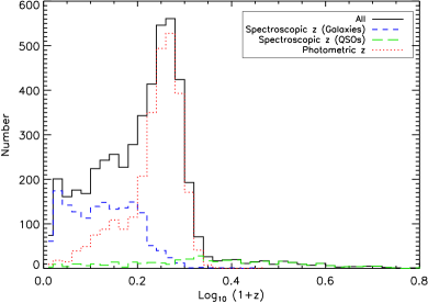
Figure 8: The redshift distribution of our cross-matched sample. The distribution for galaxies and QSOs with spectroscopic redshifts can be seen as blue and green dashed lines respectively. The distribution for objects with photometric redshifts can be seen as the red dotted line.

The integrated ($S_{{\rm int}}$) and peak ($S_{{\rm peak}}$) flux densities of the different cross-matched samples are shown in Figure 9, and span a range of fluxes from $\sim 0.2$mJy to $\sim 1$ Jy. Many of the spectroscopic and photometric cross-matches have $S_{{\rm int}}$ flux densities that are greater than their $S_{{\rm peak}}$ flux densities indicating they are extended objects. As expected most QSOs lie on the $S_{{\rm int}}=S_{{\rm peak}}$ line consistent with them being compact radio sources. The radio morphologies of our sample will be investigated in a future study.

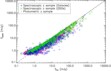
Figure 9: Comparison of the integrated and peak flux densities for the photometric cross-matched sample and spectroscopic cross-matched sample divided into galaxies and QSOs. The dotted line indicates where $S_{\rm peak}=S_{\rm int}$. QSOs tend to follow this line indicating they are compact sources.

Radio K-corrections assuming a spectral index of $\alpha=-0.7$ (where $S\propto\nu^{\alpha}$) are use to calculate radio luminosities of our samples. The redshift-luminosity distribution of our samples can be seen in Figure 10.

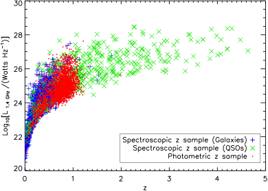
Figure 10: Radio luminosity of the sources as a function of redshift. Red points indicate objects with photometric redshifts. Objects with SDSS spectra classified as galaxies can be seen as blue crosses, and QSOs can be seen as green crosses. A spectral index of $\alpha=-0.7$ is assumed for all sources, when calculating the radio luminosity.

5 New Giant Radio Galaxies

One of the advantages of having medium depth data covering a significant area, with good surface brightness sensitivity, is that we are able to pick up rare objects such as Giant Radio Galaxies (GRGs). GRGs are a rare form of FR II galaxies and are the largest single connected structures in the Universe, with radio lobes that extend to distances of $\sim 0.7$ Mpc and beyond (Schoenmakers et al., 2001; Saripalli et al., 2005). They can also be used to probe the Inter-Galactic Medium (IGM) properties of galaxies (Malarecki et al., 2013).

During the cross-matching process we discovered three new GRGs, which can be seen in Figure 11. These would have almost certainly been missed if the matching process had been automated. The first in the upper panel of Figure 11, GRG020543.42-005029.08, appears to be a restarted ‘double-double’ radio galaxy with $2$ sets of hot spots extending in a South-West to North-East direction. No radio core is detected. The outer lobes extend across an angular diameter of $\sim 4\arcmin$, which corresponds to a projected size of $1.66$ Mpc at the spectroscopic redshift ($z=0.65$) of the host. With an integrated flux of $19.24\pm 4.39$ mJy, the object has a luminosity of $L_{\rm 1.4GHz}=4.07\pm 0.92\times 10^{25}~{}{\rm WHz^{-1}}$.

The 2nd GRG and most luminous one we have found, GRG225734.49-005231.96 (middle panel of Figure 11), extends $\sim 6.3\arcmin$ in size. The host is a galaxy at $z=0.52$, giving the GRG a projected size of $2.35$ Mpc. A total integrated flux of $62.08\pm 6.12$ mJy yields a luminosity of $L_{\rm 1.4GHz}=7.49\pm 0.74\times 10^{25}~{}{\rm WHz^{-1}}$.

The $3$rd GRG, GRG223110.11+010201.00, consists of two large diffuse lobes extending $\sim 8\arcmin$ in a North-South direction. The host galaxy has a photometric redshift $z=0.23$, which gives the object a projected size of $\sim 1.77$ Mpc. The object has an integrated flux of $112.61\pm 22.52$ mJy corresponding to a luminosity of $L_{\rm 1.4GHz}=1.91\pm 0.38\times 10^{25}~{}{\rm WHz^{-1}}$.

Follow up observations of these objects conducted at other radio frequencies would allow spectral indices and curvature to be determined, from which the ages of the jets could be deduced.

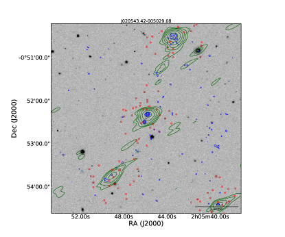
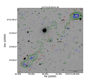
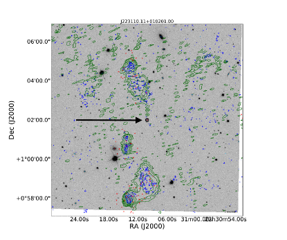
Figure 11: Three new Giant Radio Galaxies discovered during the cross-matching process. The radio contours and greyscale images are the same as Figure 2. The images are centred on the host of the GRG. The black arrow indicates the core of the third GRG.

6 Separating AGN and Star-forming Galaxies

For the sources with optical spectroscopy we are able to use the method of Best & Heckman (2012) to separate the radio-loud AGN and star-forming galaxy populations. As we are only interested in spectroscopic cross-matches determined by the SDSS pipeline to be galaxies, we restrict the sample to SDSS galaxies (type $=3$ sources) and remove those classified as QSOs. To ensure we have the required emission lines to classify our galaxies, covered by the spectral range of the SDSS spectrograph, we restrict our sample to those with $z<0.85$. Applying these conditions results in a sample of $1\,518$ objects. Following the method of Best & Heckman (2012) seen in their Appendix A, we produce three different diagnostics that classify an object as either being an AGN, a star-forming galaxy or unclassified. An object that might be classified as an AGN in one diagnostic will not necessarily be classified as an AGN by the two other diagnostics. This means that there are 27 possible combinations of classification for an object, from which we deduce an overall classification.

The first of the diagnostics is the well known BPT diagram (Baldwin et al., 1981), which uses the ratio of forbidden emission lines and the Balmer series (${\rm[OIII]/H\beta}$ and ${\rm[NII]/H\alpha}$) to distinguish the two populations. Here we use the division line of Kewley et al. (2001), below which star-forming galaxies are found, given by:

$$\log_{10}{\rm([OIII]/H\beta)}=1.31+0.61\log_{10}{\rm([NII]/H\alpha)}+0.05.$$ (1)

Emission line strengths from the Portsmouth reductions (Thomas et al., 2013) of the SDSS DR14 spectra were used to determine the ${\rm[OIII]/H\beta}$ and ${\rm[NII]/H\alpha}$ line ratios. To ensure a thorough classification using this method we only include objects where each of the $4$ emission lines have a ${\rm SNR}>3.0$. This meant that $660$ objects could be classified using this diagnostic, which resulted in $456$ AGN and $204$ star-forming galaxies. The remaining $858$ objects were left unclassified using this diagnostic.

The second diagnostic is the H$\alpha$ luminosity ($L_{{\rm H\alpha}}$) versus radio luminosity ($L_{{\rm Radio}}$) method. For star-forming galaxies the ${\rm H\alpha}$ and radio luminosities should correlate, as both trace the star formation rate (SFR) of a galaxy. AGN on the other hand produce an excess of radio emission and therefore have higher radio luminosities. A clear division between star-forming galaxies and AGN can be seen in Figure  13 and we separate the populations along the line:

$$\log_{10}(L_{{\rm H\alpha}})=1.12\times\log(L_{{\rm Radio}})-16.5$$ (2)

The secondary axes on Figure 12 show estimates of the SFRs from the range of radio and ${\rm H\alpha}$ luminosities covered. The radio luminosity was converted to a radio SFR ($\rm SFR_{\rm Radio}$) using the conversion found in Condon (1992). The ${\rm SFR_{H\alpha}}$ scale was estimated using the conversion of Gallego et al. (1995). As the ${\rm H\alpha}$ luminosities displayed here are uncorrected for fibre aperture effects, an average SDSS fibre aperture correction factor of $0.65$ dex, as found by Duarte Puertas et al. (2017), was applied to the ${\rm SFR_{\rm H\alpha}}$ luminosity scale. From this it can clearly be seen that star-forming galaxies closely follow the line where the ${\rm SFR_{\rm radio}}$ and ${\rm SFR_{\rm H\alpha}}$ are equal (solid black line), whereas AGN do not. Here we only use galaxies with a ${\rm H\alpha}$ flux detected with ${\rm SNR}>3.0$, which meant a subset of $942$ from the initial sample of $1\,518$ spectroscopic sources could be classified in this way. This resulted in $587$ AGN and $355$ star-forming galaxies, with the remaining $576$ being unclassified with this method.

The third diagnostic uses the strength of the $4000$ Å break and the ratio of radio luminosity and $M^{*}$ of a galaxy, in the so called ‘$D_{4000}$ versus $L_{{\rm Radio}}/M^{*}$’ method, developed by Best et al. (2005b). Here the stellar masses used were taken from the Portsmouth reductions of the SDSS DR14 spectra (Thomas et al., 2013), using templates for passively evolving galaxies. AGN in general have a stronger $4000$ Å break and have larger $L_{{\rm Radio}}/M^{*}$ values due to their excess radio emission. For star-forming galaxies $L_{{\rm Radio}}/M^{*}$ and $D_{4000}$ trace the specific SFR of the galaxy and hence follow a locus on the diagram. Here we divide AGN and star-forming galaxies in the same way as Best et al. (2005b). Galaxies are divided along the $D_{4000}$ track of a galaxy with an exponentially declining SFR with an e-folding time of $3$ Gyr, shifted upwards by $0.225$. This track was produced from the Bruzual & Charlot (2003) galaxy evolution models. The $D_{4000}$ measurements for $885$ objects were available, allowing the sample to be divided into $577$ AGN and $308$ star-forming galaxies, leaving $633$ unclassified.

The resulting diagnostic plots can be seen in Figures 12, 13 and 14. Those classified overall as AGN and star-forming galaxies can be seen as the red and blue points respectively. A full breakdown of the $27$ possible combinations of the classifications from each diagnostic can be seen in Table 1.

Table 1: The number of sources classified as radio-loud AGN and star-forming galaxies for each of diagnostics and the overall classification adopted from all three. We use the same rationale of the overall classifications as Best et al. (2015). ‘AGN’,‘SF’ and ‘??’ denotes that the objects are classified as AGN, star-forming galaxies or unclassified respectively, for each of the three methods.

D4000 v $L_{\rm Radio}/M^{*}$	BPT	$L_{\rm H\alpha}$ v $L_{\rm Radio}$	Overall Classification	Number of sources
AGN	AGN	AGN	AGN	$145$
AGN	AGN	??	AGN	$0$
AGN	AGN	SF	AGN	$31$
AGN	??	AGN	AGN	$150$
AGN	??	??	AGN	$229$
AGN	??	SF	AGN	$7$
AGN	SF	AGN	AGN	$11$
AGN	SF	??	-	$0$
AGN	SF	SF	SF	$4$
??	AGN	AGN	AGN	$138$
??	AGN	??	AGN	$0$
??	AGN	SF	SF	$17$
??	??	AGN	AGN	$120$
??	??	??	AGN a	$333$
??	??	SF	SF	$1$
??	SF	AGN	-	$13$
??	SF	??	-	$0$
??	SF	SF	SF	$11$
SF	AGN	AGN	AGN	$7$
SF	AGN	??	-	$0$
SF	AGN	SF	SF	$118$
SF	??	AGN	AGN	$1$
SF	??	??	SF	$14$
SF	??	SF	SF	$3$
SF	SF	AGN	SF	$2$
SF	SF	??	SF	$0$
SF	SF	SF	SF	$163$

• As all of the diagnostics are inconclusive for these objects, we assume they are radio-loud AGN, as they have luminosities of $\log_{10}L_{\rm 1.4GHz}/{\rm WHz^{-1}}>24.5$, in the same way as Best & Heckman (2012).

We adopt the same combinations of classifications to determine the overall classification of an object as Best & Heckman (2012). Objects with $\log_{10}(L_{\rm 1.4GHz}/{\rm WHz^{-1}})>24.5$ were also classified as AGN, which meant that $5$ objects initially classed as star-forming galaxies were reclassified as AGN.

Overall we find $340$ star-forming galaxies and $1\,178$ AGN from the three diagnostics. As an extra check the spectrum of each object was visually classified in a similar way to Mauch & Sadler (2007) and Prescott et al. (2016). Spectra with strong, narrow, Balmer emission lines produced by Hii regions were classified as star-forming galaxies. In contrast, we classify objects as AGN if they exhibit pure absorption line spectra typical of elliptical galaxies, broadened emission lines (Type 1 AGN) or strong nebula emission lines compared to the Balmer series (Type 2 AGN). From the initial sample of $1\,518$ objects, this process resulted in $1\,190$ AGN and $328$ star-forming galaxies, which agree with the numbers found using the diagnostics described above.

We note that the BPT diagram has a much larger contamination of SFGs in the AGN region than the other diagnostic diagrams, which may indicate a significant population of “hybrid” objects, where there is star formation alongside the AGN activity. In order to investigate this further, full spectral-energy distribution fitting would be needed to evaluate the relative contributions to the total energy budget.

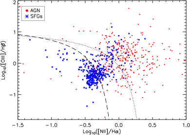
Figure 12: BPT diagram for the spectroscopic objects within $z<0.85$, with the required emission lines detected at a $S/N>3$. AGN and star-forming galaxies are separated by the dashed line from Kewley et al. (2001). Objects above this line but below the dotted line are considered to be composite galaxies in Kauffmann et al. (2003). Here we plot overall classifications determined from the three diagnostics. AGN can be seen as red circles and star-forming galaxies as blue stars.

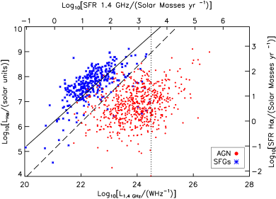
Figure 13: $\rm H\alpha$ Luminosity - Radio Luminosity plot used as the 2nd diagnostic to divide AGN and star-forming galaxies. The dashed line shows the division used. The vertical dotted line indicates the luminosity ($\log_{10}(L_{\rm Radio}/\rm{WHz^{-1}})=24.5$) above which all objects should be AGN, as found by Best et al. (2012). Again overall AGN/SFG classifications determined from the three diagnostics are plotted. AGN can be seen as red circles and star-forming galaxies as blue stars. The black solid line indicates where estimates of the star-formation rates determined from radio and ${\rm H\alpha}$ luminosities are equal.

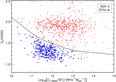
Figure 14: Dn₄₀₀₀ against the ratio $L_{\rm Radio}/M_{*}$ for the spectroscopic sample. The solid line shows the track of a star-forming galaxies produced by Bruzual & Charlot (2003) shifted by $0.225$ used to separate AGN and star-forming galaxies. Objects above this line are classified as AGN. As in the previous diagnostic plots, those classified overall as AGN can be seen as red circles and star-forming galaxies as blue stars.

6.1 High and Low Excitation Radio Galaxies

We use optical spectra to further separate the radio-loud AGN population into high and low excitation radio galaxies (HERGs and LERGs). As in Laing et al. (1994), Prescott et al. (2016) and Ching et al. (2017) we make use of the $5007$Å ${\rm[OIII]}$ emission line, identifying HERGs as those objects that have measurable ${\rm[OIII]}$ equivalent widths (EW) $>5$ Åwith a ${\rm SNR}>3$. The rest were classifed as LERGs. Applying this condition results in a sample of $57$ HERGs and $1\,121$ LERGs. In Figure 15 we show the radio luminosity of the different radio populations as a function of redshift. As expected star-forming galaxies are the dominant population below $z<0.2$. HERGs and LERGs can be seen throughout the redshift range covered here, with HERGs being generally more radio luminous than LERGs. A comprehensive study of the HERG and LERG populations of radio-loud AGN, including their accretion rate and mechanical and radiative luminosities, is covered in Whittam et al. (2018).

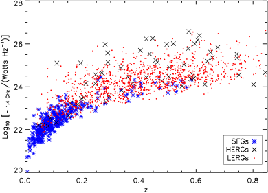
Figure 15: The radio luminosity of the radio sources with spectroscopic counterparts as a function of redshift. SFGs can be seen as blue stars, HERGs as black crosses and LERGs as red circles. Star-forming galaxies become the dominant population at low redshift. HERGs are on average more radio luminous than the LERGs.

7 Control Matched HERGs and LERGs

In this section we investigate the host properties of the HERGs and LERGs in the sample with spectroscopic redshifts of $z<0.4$, matched in $M^{*}$, radio luminosity and redshift, to take into account the selection effects of the radio and optical surveys we have used. In particular we investigate how the rest-frame $(g-r)_{0}$ colour, concentration index given by $C=r_{90}/r_{50}$ (where $r_{90}$ and $r_{50}$ are the radii containing $90$ and $50$ per cent of the Petrosian flux) and the projected physical size of the galaxy, $R_{50}$, determined from $r_{50}$. Rest-frame colours were calculated using rest-frame magnitudes calculated by kcorrect v4.3 (Blanton & Roweis, 2007).

We use a similar method as Best & Heckman (2012) and Ching et al. (2017) to produce a control matched sample of HERGs and LERGs. As the majority of our objects are LERGs, for each HERG we look for $3$ LERGs which have $\lvert\Delta\log_{10}L_{\rm 1.4GHz}\rvert<0.25$, $\lvert\Delta\log_{10}M^{*}\rvert<0.15$ and $\lvert\Delta z\rvert<0.03$. If at least $3$ LERGs satisfy the criteria then $3$ LERGs are randomly selected to belong to the control sample. Any HERGs that have $2$ or fewer matched LERGs are rejected from the analysis. We also ensure the control LERGs are unique.

Histograms for both matched and unmatched properties of the HERGs and control matched LERGs can be seen in Figure 16. Mean values of each parameter for the HERGs and LERGs can be seen as vertical lines which highlight the similarities in stellar mass, radio luminosity and redshift that are expected from a robust control sample. Small differences in the mean rest-frame colour and concentration can be seen. We see no evidence for HERGs and LERGs having physically different sizes.

For robustness we conduct a two sample KS-tests on $1\,000$ iterations of the randomly matched control samples. The probabilities that the HERG and LERG samples are drawn from the same distrubution can be seen in Table 2. These probabilities are high for the stellar mass, radio luminosity and redshift distributions indicating we have produced a sensible control match of LERGs. However, for the unmatched parameters the probabilities are also high, suggesting that we cannot determine whether they are drawn from differing underlying distributions.

However, we do find that, in this limited sample, the LERGs are slightly redder than HERGs by $(g-r)_{0}\sim 0.1$ indicating they are more dominated by older stellar populations. They are also are more concentrated on average, with concentration values of $C\sim 3$ that are typical of early-type or elliptical galaxies (Shimasaku et al., 2001). Using much larger galaxy samples Best & Heckman (2012) and Ching et al. (2017) find similar results, regarding colour and concentration, but also observe that LERGs are larger in physical size than HERGs. We would require a much larger sample to confirm these very tentative results.

Differences in stellar mass and stellar age for the HERG and LERG populations, along with their accretion rates and potential feedback effects, are discussed in Whittam et al. (2018).

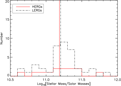
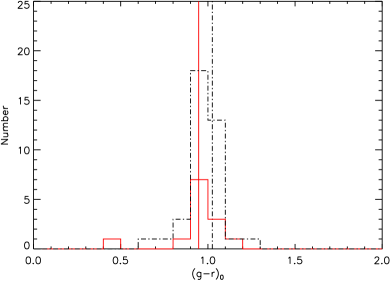
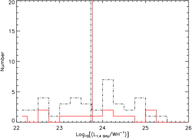
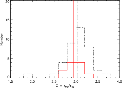
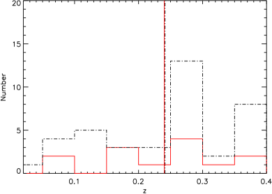
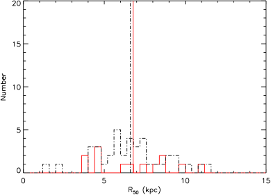
Figure 16: Histograms comparing the host properties of HERGs (solid red lines) and LERGs (black dashed lines) within $z=0.4$. The vertical lines show mean values for both the HERGs and LERGs. On the left-hand panels we show histograms comparing the control matched properties of $M^{*}$, radio luminosity and redshift, which show there are no significant differences between the HERGs and LERGs as expected. On the right-hand panels we show histrograms comparing the rest-frame $(g-r)$ colour, concentration index $(C=r_{90}/r_{50})$ and the projected galaxy size determined light radius $(R_{50})$ measurement. Differences can be seen here which indicate LERGs are slightly redder and more concentrated than HERGs of similar mass, radio luminosity and redshift.

Table 2: KS test probabilities between the control matched HERG and LERG samples for the different galaxy properties. The values are the mean from 1 000 iterations of randomly selected control matched LERGs.

Parameter	K-S Test Probability
Matched Parameters
Stellar Mass ($M^{*}$)	$0.86$
Radio Luminosity ($L_{\rm 1.4GHz}$)	$0.99$
Redshift ($z$)	$0.99$
Unmatched Parameters
Rest Frame Colour $(g-r)$	$0.42$
Concentration Index ($C=r_{90}/r_{50}$)	$0.38$
Projected Size ($R_{50}$)	$0.78$

8 $K-z$ relation

8.1 VICS82 $K-z$ relation

The $K$-band magnitudes of radio galaxies have long been known to show a tight correlation with redshift, in what is known as the ‘$K-z$ relationship’ (Lilly & Longair, 1984; Eales et al., 1997; Jarvis et al., 2001; Willott et al., 2003). This trend is believed to arise as consequence of radio galaxies being a population of massive galaxies that have formed early in the Universe (with a formation redshift $z_{f}>5.0$), and have undergone passive evolution ever since. In order to investigate this, we match our catalogue with $K_{s}$ band data from the Vista-CFHT Stripe 82 (VICS82) near-infrared survey (Geach et al., 2017). Matching the optical positions of our spectroscopic catalogue with the VICS82 public catalogue, using a matching radius of $2\arcsec$, results in $996$ cross-matches, with reliable spectra.

Figure 17 shows the $K-z$ relation for $234$ star-forming galaxies (blue stars), $38$ HERGs (red crosses) and $689$ LERGs (red circles), plotted along with the entire VICS82 sample of objects covering the same region of sky as the radio survey (grey dots). Here $K_{s}$ band magnitudes are total (‘AUTO’) magnitudes derived from SExtractor Bertin & Arnouts (1996).

It can clearly be seen that the AGN $K_{s}$-band magnitudes follow a tight correlation with redshift. Star-forming galaxies on the other hand deviate from this relationship and show considerable scatter above the $K-z$. This is not unexpected as star-forming galaxies are ungoing current star formation and are not dominated by older stellar populations which predominanly produce $K$-band light. Fitting a polynomial of the form: $K=A(\log_{10}z)^{2}+B\log_{10}z+C$ to the LERG population with $z>0.1$ only, yields constants of $A=0.17$, $B=4.42$ and $C=18.79$. This is consistent with the $K-z$ relation from Willott et al. (2003) corrected from Vega to AB magnitudes. This can be seen as the dashed line in Figure 17, which has the form: $K=-0.31(\log_{10})^{2}+4.53\log_{10}z+19.19$.

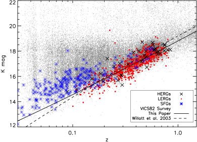
Figure 17: $k-z$ relation produced from matching our spectroscopic cross-matched sample to the VICS82 survey. Here star-forming galaxies (blue stars), HERGs (black crosses) and LERGs (red circles), are plotted along with the entire VICS82 sample of objects covering the same region of sky as the radio survey (grey dots).

8.2 WISE $3.4\mu$m -$z$ relation

Mid-Infrared data from the Wide-field Infrared Survey Explorer (WISE; Wright et al., 2010) has also been observed to correlate with redshift (Gürkan et al., 2014; Glowacki et al., 2017), especially the W1 $3.4\mu$m band, which can essentially be used as a proxy for the $K$-band.

Matching the optical postions of our spectroscopic sources with $z<0.85$ and z warning$=0$ to the nearest object in the All-Sky WISE catalogue within $2\arcsec$, results in a sample of $1523$ objects. This WISE matched sample contains $324$ star-forming galaxies, $1023$ LERGs, $56$ HERGs and $120$ QSOs.

Figure 18 shows the W1 (Vega) magnitudes of the HERG and LERG populations of AGN as a function of redshift. As with the $K-z$ relation above, we fit the LERG population with a 2nd order polynomial (solid line), which yields a line of best fit of $W1=-0.91(\log_{10}z)^{2}+1.41\log_{10}z+15.50$. This is very similar to the line of best fit found by Glowacki et al. (2017) of $W1=-0.68(\log_{10}z)^{2}+1.82\log_{10}z+15.74$ (dashed line), using LERGs from the Large Area Radio Galaxy Evolution Spectroscopic Survey (LARGESS) sample of radio galaxies. Gürkan et al. (2014) probe galaxies at higher redshifts and luminosities than our sample, which may explain why their line of best fit of $W1=-0.13(\log_{10}z)^{2}+2.85\log_{10}z+15.46$ (dotted line in Figure 18) is a poorer fit to our sample. Indeed, many previous studies of the host galaxies of radio galaxies has shown that there is evidence for a correlation between radio luminosity and galaxy mass (e.g. Jarvis et al., 2001; McLure et al., 2004). Given that our sample is around three orders of magnitude more sensitive than the sample used by Gürkan et al. (2014), it is not surprising that the $K-z$ relation is also offset.

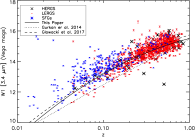
Figure 18: $K-z$ relation of WISE matched AGN and star-forming galaxies, from our cross-matched spectroscopic sample, using W1 ($3.4\mu$m) band as a proxy for the $K$ band. HERGs can be seen as the black crosses, LERGs can be seen as red circles and star-forming galaxies as blue stars. The solid black line indicates our line of best fit to the LERGs. The line of best fit found by Gurkan et al. 2014 can be seen as the dotted line. The line of best fit as found by Glowacki et al. (2017) for LERGs can be seen as the dashed line.

9 WISE colours of the radio populations

In this section we discuss the WISE colours of the HERG and LERG populations of AGN, star-forming galaxies and quasars. WISE colour-colour diagrams, first produced by Wright et al. (2010), have been shown to be an important tool for distinguishing the dominant source of Mid-Infrared (MIR) emission from objects. $W1-W2$ v $W2-W3$ is one such diagram, as shown in Figure 19. Here redder $W1-W2$ colours indicate a greater contribution of non-stellar emission from AGN and $W2-W3$ is correlated to the specific star-formation rate (sSFR), with redder colours indicating lower sSFR (Donoso et al., 2012). Note that we use Vega magnitudes in this figure.

As expected, the majority of QSOs and HERGs in Figure 19 can clearly be seen in the upper half of the figure. We find that for QSOs the $W1-W2$ colour ranges from $0.0<W1-W2<1.75$ with median of $W1-W2=0.8$. $W2-W3$ ranges from $2.14<W2-W3<4.96$ with a median of $W2-W3=3.08$. For the HERGs, the $W1-W2$ colour ranges from $-0.2<W1-W2<1.55$, with the median being $W1-W2=0.31$ and the $W2-W3$ colour ranges from $1.32<W2-W3<4.26$ with a median of $W2-W3=2.77$. We find that $80$ per cent of the QSOs and $31$ per cent of HERGs can be found above $W1-W2>0.5$, which was the line that Mingo et al. (2016) used to label QSOs. A significant number of QSOs would be missed if simply using the AGN selection criterion of $W1-W2>0.8$ for objects to a depth of $W2=15.0$, as used by Stern et al. (2012) from WISE observations of the COSMOS field.

These higher values of $W1-W2$ for the HERGs and QSOs are indicative of the presence of a hot dusty torus. The black solid lines bound a region where objects containing a dusty torus are expected to lie from the three band selected AGN sample of Mateos et al. (2012). The large spread in these colours is likely to be caused by orientation effects, different accretion rates and some element of photometric scatter for the fainter objects in the sample.

The vast majority of the LERG population ($99$ per cent) in Figure 19, can be seen below $W1-W2<0.5$ and show a range of $W2-W3$ colours from $0.2<W2-W3<4.5$. The majority of LERGs reside in the area of colour space where ‘ellipticals’ and ‘spirals’ can generally be found in the WISE colour-colour plot of Wright et al. (2010). The low values of $W1-W2$ indicate thar there is no dusty torus present in the LERG population and the low scatter in $W1-W2$ values implies that they are possibly unaffected by orientation effects, unlike the HERGs and QSOs.

Star-forming galaxies occupy the lower regions of plot along with the LERGs and have $W1-W2<0.7$ but have much bluer $W2-W3$ colours (the mean $W2-W3=3.79$ as opposed to the LERGs with $W2-W3=2.35$). The bluest star-forming galaxies (with $W2-W3>4$) appear where ULIRGS and starbursting galaxies reside in Wright et al. (2010). This ties together with our most rapidly star-forming galaxies having typical SFRs of $10^{3}{\rm M_{\odot}yr}^{-1}$ (see Figure 13).

The regions occupied by the different populations of radio sources, seen in Figure 19, appear to be in good agreement with the findings of Gürkan et al. (2014) using a combined sample of AGN from the 3CRR, 2Jy, 6CE and 7CE surveys, and the results from the LARGESS sample of AGN (Ching et al., 2017).

The host properties of the LERGs and HERGs seen in the previous sections are consistent with the WISE results in this section. LERGs are observed to be a population of massive, passively evolving galaxies, that have formed early in the Universe. These would have long since depleted their reservoir of cold gas, which would be necessary for efficient accretion to occur and allow the formation of a dusty torus in the accretion disk. In the absence of a cold gas reservoir, the radio emission in LERGs is produced from the slow accretion of hot reservoir of gas (Hardcastle et al., 2007; Janssen et al., 2012).

HERGs on the other hand are bluer galaxies, are still undergoing star formation and are more gas rich. This supply of cold gas is accreted onto the central black hole at a more efficient rate, which allows the formation of an optically thick and geometrically thin dusty torus (e.g. Shakura & Sunyaev 1973). The wide range of WISE colours seen in the HERGs is most plausibly due to the dusty torus being observed at different viewing angles, and a range of accretion rates on to different mass black holes, which would result in a large spread of dust temperatures within the sample.

The picture that HERGs and LERGs are undergoing different accretion modes is also reflected in the the differences in the evolution of the luminosity functions of HERGs and LERGs. HERGs are seen to rapidly evolve out to redshift of $z\sim 1$ Pracy et al. (2016), whereas LERGs show little or no evidence of evolution Clewley & Jarvis (2004); Best et al. (2014); Pracy et al. (2016).

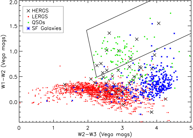
Figure 19: WISE colour-colour diagram for our sample of cross-matches with spectroscopic redshifts $z<0.85$. LERGs can be seen as red circles, HERGs as black crosses, QSOs as green circles and star-forming galaxies as blue stars. The black solid lines bound a region where objects containing a dusty torus are expected to lie from the sample of Mateos et al. (2012).

10 Conclusions

We have combined spectroscopic and photometric optical data from the SDSS with 1.4 GHz radio observations conducted as part of the Stripe 82 1-2GHz VLA snapshot survey of Heywood et al. (2016). From cross-matching the datasets via visual inspection we have produced a catalogue of $4\,795$ objects containing a mixture of star-forming galaxies, radio-loud AGN and quasars. Our main results can be summarised as follows:

• We have cross-matched a sample of $11\,768$ radio components with optical SDSS counterparts. The final catalogue includes a cross-matched sample of $1\,996$ objects with spectroscopic redshifts and $2\,799$ objects with photometric redshifts from the catalogue of Reis et al. (2012).

• We have discovered three new Giant Radio Galaxies in Stripe 82, which would otherwise have been missed using automated cross-matching methods. (Fig. 11).

• For galaxies with spectroscopic redshifts of $z<0.85$ we divide our sample into star-forming galaxies and AGN using the same three diagnostics as Best & Heckman (2012), resulting in a sample of $1\,178$ AGN and $340$ star-forming galaxies. Using [OIII] $5007$Å measurements, the radio-loud AGN population can then be divided into a sample of $57$ HERGs and $1\,121$ LERGs.

• From a control sample of HERGs and LERGs matched on stellar mass, radio luminosity and redshift, we find that the sizes, colours and concentration index of LERGs at $z<0.4$ are indisinguishable to the HERGs. Although on average the LERGs are slightly more likely to be massive, passive, early type galaxies. (Fig. 16).

• For the LERG population, we observe the $K-z$ relationship, after matching the optical positions of our spectroscopic sample to near-infrared VICS82 data. Matching the positions to WISE photometry yields a similar relationship, which is consistent with other recent results. The observed $K-z$ relationship provides further evidence that LERGs are a population of massive, passive galaxies with an early formation time. (Figs. 17 and 18).

• We produce a WISE colour-colour diagram for the different radio populations. QSOs, HERGs, LERGs and star-forming galaxies all reside in different regions of the diagram (Fig. 19). The HERGs and QSOs show MIR colours consistent with being a population of objects which have a dusty torus that are being observed at different orientations. LERGs on the other-hand are more homogenous population without a dusty torus and do not display evidence of orientation effects.

10.1 Future Work

With this large cross-matched radio dataset, covering a large area of $100$ sq degrees and going to depths of $88$ $\muup$Jy, a number of future studies to probe the nature of the different radio populations will now be possible. These will include:

• An investigation into the host properties of LERG and HERG populations of radio-loud AGN, and how their accretion rates vary (See Whittam et al. (2018)).

• Determining the evolution of star-forming galaxies and AGN from the determination of luminosity functions, as well as the evolution of QSOs.

• Determining the stellar mass function of galaxies which will allow the AGN fraction as a function of stellar mass to be investigated.

• Measuring the Far-Infrared Radio correlation, from combining the sample with data from the Herschel Extragalactic Legacy Project (HELP, Vaccari, 2016).

• Determining the morphologies of the radio sources using machine learning techniques, as this sample could also be used as an excellent training set for future surveys.

• Investigating the enviroments and clustering of the radio-loud AGN population.

References

- Abolfathi et al. (2017) Abolfathi B., et al., 2017, preprint, (arXiv:1707.09322)
- Adelman-McCarthy et al. (2006) Adelman-McCarthy J. K., et al., 2006, ApJS, 162, 38
- Annis et al. (2014) Annis J., et al., 2014, ApJ, 794, 120
- Baldwin et al. (1981) Baldwin J. A., Phillips M. M., Terlevich R., 1981, PASP, 93, 5
- Becker et al. (1995) Becker R. H., White R. L., Helfand D. J., 1995, ApJ, 450, 559
- Bertin & Arnouts (1996) Bertin E., Arnouts S., 1996, A&AS, 117, 393
- Best & Heckman (2012) Best P. N., Heckman T. M., 2012, MNRAS, 421, 1569
- Best et al. (2005a) Best P. N., Kauffmann G., Heckman T. M., Ivezić Ž., 2005a, MNRAS, 362, 9
- Best et al. (2005b) Best P. N., Kauffmann G., Heckman T. M., Ivezić Ž., 2005b, MNRAS, 362, 9
- Best et al. (2014) Best P. N., Ker L. M., Simpson C., Rigby E. E., Sabater J., 2014, MNRAS, 445, 955
- Blanton & Roweis (2007) Blanton M. R., Roweis S., 2007, AJ, 133, 734
- Bruzual & Charlot (2003) Bruzual G., Charlot S., 2003, MNRAS, 344, 1000
- Cheung (2007) Cheung C. C., 2007, AJ, 133, 2097
- Ching et al. (2017) Ching J. H. Y., et al., 2017, MNRAS, 464, 1306
- Clewley & Jarvis (2004) Clewley L., Jarvis M. J., 2004, MNRAS, 352, 909
- Colless et al. (2001) Colless M., et al., 2001, MNRAS, 328, 1039
- Condon (1992) Condon J. J., 1992, ARA&A, 30, 575
- Condon et al. (1998) Condon J. J., Cotton W. D., Greisen E. W., Yin Q. F., Perley R. A., Taylor G. B., Broderick J. J., 1998, AJ, 115, 1693
- Dawson et al. (2013) Dawson K. S., et al., 2013, AJ, 145, 10
- Donoso et al. (2012) Donoso E., et al., 2012, ApJ, 748, 80
- Duarte Puertas et al. (2017) Duarte Puertas S., Vilchez J. M., Iglesias-Páramo J., Kehrig C., Pérez-Montero E., Rosales-Ortega F. F., 2017, A&A, 599, A71
- Eales et al. (1997) Eales S., Rawlings S., Law-Green D., Cotter G., Lacy M., 1997, MNRAS, 291, 593
- Eisenstein et al. (2001) Eisenstein D. J., et al., 2001, AJ, 122, 2267
- Fan et al. (2015) Fan D., Budavári T., Norris R. P., Hopkins A. M., 2015, MNRAS, 451, 1299
- Gallego et al. (1995) Gallego J., Zamorano J., Aragon-Salamanca A., Rego M., 1995, ApJ, 455, L1
- Geach et al. (2017) Geach J. E., et al., 2017, ApJS, 231, 7
- Glowacki et al. (2017) Glowacki M., Allison J. R., Sadler E. M., Moss V. A., Jarrett T. H., 2017, preprint, (arXiv:1709.08634)
- Gunn et al. (1998) Gunn J. E., et al., 1998, AJ, 116, 3040
- Gürkan et al. (2014) Gürkan G., Hardcastle M. J., Jarvis M. J., 2014, MNRAS, 438, 1149
- Hardcastle et al. (2007) Hardcastle M. J., Evans D. A., Croston J. H., 2007, MNRAS, 376, 1849
- Hardcastle et al. (2016) Hardcastle M. J., et al., 2016, MNRAS, 462, 1910
- Heywood et al. (2016) Heywood I., et al., 2016, MNRAS, 460, 4433
- Hodge et al. (2011) Hodge J. A., Becker R. H., White R. L., Richards G. T., Zeimann G. R., 2011, AJ, 142, 3
- Hogg et al. (2001) Hogg D. W., Finkbeiner D. P., Schlegel D. J., Gunn J. E., 2001, AJ, 122, 2129
- Ilbert et al. (2006) Ilbert O., et al., 2006, A&A, 457, 841
- Janssen et al. (2012) Janssen R. M. J., Röttgering H. J. A., Best P. N., Brinchmann J., 2012, A&A, 541, A62
- Jarvis et al. (2001) Jarvis M. J., Rawlings S., Eales S., Blundell K. M., Bunker A. J., Croft S., McLure R. J., Willott C. J., 2001, MNRAS, 326, 1585
- Jarvis et al. (2013) Jarvis M. J., et al., 2013, MNRAS, 428, 1281
- Jarvis et al. (2017) Jarvis M. J., et al., 2017, preprint, (arXiv:1709.01901)
- Jones et al. (2004) Jones D. H., et al., 2004, MNRAS, 355, 747
- Kewley et al. (2001) Kewley L. J., Heisler C. A., Dopita M. A., Lumsden S., 2001, ApJS, 132, 37
- Kroupa (2001) Kroupa P., 2001, MNRAS, 322, 231
- Laing et al. (1994) Laing R. A., Jenkins C. R., Wall J. V., Unger S. W., 1994, in Bicknell G. V., Dopita M. A., Quinn P. J., eds, Astronomical Society of the Pacific Conference Series Vol. 54, The Physics of Active Galaxies. p. 201
- Lilly & Longair (1984) Lilly S. J., Longair M. S., 1984, MNRAS, 211, 833
- Malarecki et al. (2013) Malarecki J. M., Staveley-Smith L., Saripalli L., Subrahmanyan R., Jones D. H., Duffy A. R., Rioja M., 2013, MNRAS, 432, 200
- Mateos et al. (2012) Mateos S., et al., 2012, MNRAS, 426, 3271
- Mauch & Sadler (2007) Mauch T., Sadler E. M., 2007, MNRAS, 375, 931
- McAlpine et al. (2012) McAlpine K., Smith D. J. B., Jarvis M. J., Bonfield D. G., Fleuren S., 2012, MNRAS, 423, 132
- McLure et al. (2004) McLure R. J., Willott C. J., Jarvis M. J., Rawlings S., Hill G. J., Mitchell E., Dunlop J. S., Wold M., 2004, MNRAS, 351, 347
- McMullin et al. (2007) McMullin J. P., Waters B., Schiebel D., Young W., Golap K., 2007, in Shaw R. A., Hill F., Bell D. J., eds, Astronomical Society of the Pacific Conference Series Vol. 376, Astronomical Data Analysis Software and Systems XVI. p. 127
- Mingo et al. (2016) Mingo B., et al., 2016, MNRAS, 462, 2631
- Mohan & Rafferty (2015) Mohan N., Rafferty D., 2015, PyBDSF: Python Blob Detection and Source Finder, Astrophysics Source Code Library (ascl:1502.007)
- Norris et al. (2011) Norris R. P., et al., 2011, Publ. Astron. Soc. Australia, 28, 215
- Ocran et al. (2017) Ocran E. F., Taylor A. R., Vaccari M., Green D. A., 2017, MNRAS, 468, 1156
- Padovani et al. (2011) Padovani P., Miller N., Kellermann K. I., Mainieri V., Rosati P., Tozzi P., 2011, ApJ, 740, 20
- Pracy et al. (2016) Pracy M. B., et al., 2016, MNRAS, 460, 2
- Prescott et al. (2016) Prescott M., et al., 2016, MNRAS, 457, 730
- Reis et al. (2012) Reis R. R. R., et al., 2012, ApJ, 747, 59
- Roberts et al. (2018) Roberts D. H., Saripalli L., Wang K. X., Sathyanarayana Rao M., Subrahmanyan R., KleinStern C. C., Morii-Sciolla C. Y., Simpson L., 2018, ApJ, 852, 47
- Robitaille & Bressert (2012) Robitaille T., Bressert E., 2012, APLpy: Astronomical Plotting Library in Python, Astrophysics Source Code Library (ascl:1208.017)
- Sadler et al. (2002) Sadler E. M., et al., 2002, MNRAS, 329, 227
- Santos et al. (2017) Santos M. G., et al., 2017, preprint, (arXiv:1709.06099)
- Saripalli et al. (2005) Saripalli L., Hunstead R. W., Subrahmanyan R., Boyce E., 2005, AJ, 130, 896
- Schirmer et al. (2013) Schirmer M., Diaz R., Holhjem K., Levenson N. A., Winge C., 2013, ApJ, 763, 60
- Schoenmakers et al. (2001) Schoenmakers A. P., de Bruyn A. G., Röttgering H. J. A., van der Laan H., 2001, A&A, 374, 861
- Shakura & Sunyaev (1973) Shakura N. I., Sunyaev R. A., 1973, A&A, 24, 337
- Shimasaku et al. (2001) Shimasaku K., et al., 2001, AJ, 122, 1238
- Smith et al. (2011) Smith D. J. B., et al., 2011, MNRAS, 416, 857
- Smolčić et al. (2017) Smolčić V., et al., 2017, A&A, 602, A1
- Stern et al. (2012) Stern D., et al., 2012, ApJ, 753, 30
- Taylor & Jagannathan (2016) Taylor A. R., Jagannathan P., 2016, MNRAS, 459, L36
- Thomas et al. (2013) Thomas D., et al., 2013, MNRAS, 431, 1383
- Vaccari (2016) Vaccari M., 2016, The Universe of Digital Sky Surveys, 42, 71
- Whittam et al. (2017) Whittam I. H., Green D. A., Jarvis M. J., Riley J. M., 2017, MNRAS, 464, 3357
- Whittam et al. (2018) Whittam I. H., Prescott M., McAlpine K., Jarvis M. J., Heywood I., 2018, MNRAS
- Williams et al. (2016) Williams W. L., et al., 2016, MNRAS, 460, 2385
- Willott et al. (2003) Willott C. J., Rawlings S., Jarvis M. J., Blundell K. M., 2003, MNRAS, 339, 173
- Wright et al. (2010) Wright E. L., et al., 2010, AJ, 140, 1868
- York et al. (2000) York D. G., et al., 2000, AJ, 120, 1579
- van Haarlem et al. (2013) van Haarlem M. P., et al., 2013, A&A, 556, A2