Coexistence of weak and strong coupling with a quantum dot in a photonic molecule

Abstract

We study the emission from a molecular photonic cavity formed by two proximal photonic crystal defect cavities containing a small number (<3) of In(Ga)As quantum dots. Under strong excitation we observe photoluminescence from the bonding and antibonding modes in excellent agreement with expectations from numerical simulations. Power dependent measurements reveal an unexpected peak, emerging at an energy between the bonding and antibonding modes of the molecule. Temperature dependent measurements show that this unexpected feature is photonic in origin. Time-resolved measurements show the emergent peak exhibits a lifetime $\tau_{M}=$0.75\pm 0.1\text{\,}\mathrm{ns}$$, similar to both bonding and antibonding coupled modes. Comparison of experimental results with theoretical expectations reveal that this new feature arises from a coexistence of weak- and strong-coupling, due to the molecule emitting in an environment whose configuration permits or, on the contrary, impedes its strong-coupling. This scenario is reproduced theoretically for our particular geometry with a master equation reduced to the key ingredients of its dynamics. Excellent qualitative agreement is obtained between experiment and theory, showing how solid-state cavity QED can reveal new regimes of light-matter interaction.

I Introduction

Cavity QED (cQED) in solid-state systems Arakawa et al. (2015) is rapidly developing into a field of its own following the Nobel prize winning precedent set by atoms in microwave cavities Haroche (2013). Unlike their atomic counterparts, solid state systems provide great flexibility to engineer ad hoc structures in complex geometries Kuruma et al. (2016). Among the possible architectures, photonic crystal (PhC) nanostructures triplet peak structure provide the flexibility to probe cQED phenomena in non-standard configurations Lodahl et al. (2015). Due to their planar geometry, they provide a promising platform for future integrated quantum photonic devices O’Brien et al. (2009). High quality (Q) factors combined with the ultra-small mode volumes of PhC cavities allows cQED to be studied in the few photon limit Soljačić and Joannopoulos (2004); Englund et al. (2007); Fushman et al. (2008); Englund et al. (2010); Volz et al. (2012); Englund et al. (2012); Choi et al. (2017). Most of the cQED experiments performed to date using PhCs have been performed using a single cavity. In this work, by coupling two proximal nano-resonators to form a photonic molecule (PM) Bayer et al. (1998); Atlasov et al. (2008); Dousse et al. (2010a); Chalcraft et al. (2011); Atlasov et al. (2011); Majumdar et al. (2012), we open the way to explore new degrees of freedom with potential for entirely new functionalities. For example the energy splitting of the PM modes can be tuned via geometric parameters during fabrication or tuning using photochromic materials or nanoelectromechanical systems Cai et al. (2013); Haddadi et al. (2014); Kapfinger et al. (2015); Du et al. (2016). This allows the simultaneous enhancement of two different transitions and establishing of coupling between two quantum emitters separated by distances comparable to the optical wavelength Dousse et al. (2010b, a). Recent theoretical proposals taking advantage of coupled resonators suggest new applications, such as the generation of optimized Gaussian amplitude squeezing with very small Kerr nonlinearities Liew and Savona (2010), the generation of bound photon-atom states Longo et al. (2010) or the full optical coherent control of vacuum Rabi oscillations Bose et al. (2014). Photonic crystal molecules are also of great interest for solid-state implementations of photonic quantum simulators Hartmann et al. (2006); Greentree et al. (2006); Houck et al. (2012). However, to date, only a handful of experiments have been performed using PMs, exploring non-linear effects such as sum frequency generation Rivoire et al. (2010, 2011) or parametric oscillation Armstrong et al. (1962); Diederichs et al. (2006), despite the early demonstration of the up-conversion excitation in bulk GaAs Kammerer et al. (2001), and enhanced efficiencies using planar microcavities Diederichs et al. (2006); Xu et al. (2014).

Here, we investigate the linear and non-linear properties of an individual PM formed by two coupled PhC cavities doped with self assembled quantum dots (QDs). By performing photoluminescence (PL) and PL-excitation (PLE) spectroscopy we provide clear evidence for the photonic coupling of the two cavities. In power dependent PL-measurements we observe bonding- (B) and antibonding- (AB) like modes of the PM at energies that are in excellent quantitative agreement with finite-difference time-domain (FDTD) simulations. Surprisingly, we observe an additional unexpected peak (W) that emerges precisely between B and AB when the system is subjected to strong excitation. Time-integrated PL measurements performed as a function of the lattice temperature and time-resolved spectroscopy reveal that this additional unexpected peak is primarily photonic in origin. We explain this unexpected feature as a zero-dimensional counterpart of phonon-sidebands where an optical transition occurs in a lattice environment which is altered by the emission itself, making it dependent on whether the emitter is in its ground or excited state. Here, in addition to substituting the phonon bath by a two-level system, the emission itself is from a strongly-coupled system which features a Rabi doublet instead of a single line. This results in a peculiar phenomenology where an anomalous peak seem to grow in between a conventional Rabi doublet, that our interpretation shows results from a coexistence of weak and strong-coupling, as an extreme case where the molecule finds itself in an environment that either exposes or shields it from an additional decay channel which results in spoiling or preserving its coherent Rabi dynamics. A quantum-optical model that couples a QD to the PM through phonon-mediated transitions captures this phenomenon and provides a fundamental picture of this otherwise peculiar mechanism. Our result shows that the highly complex configurations one can engineer in the solid state provide interesting variations on the basic themes of light-matter interactions.

II Fabrication and Experiment

The sample was grown using molecular beam epitaxy on a $350\text{\,}\mathrm{\SIUnitSymbolMicro m}$ thick [100] orientated GaAs wafer. After depositing a $300\text{\,}\mathrm{nm}$ thick GaAs buffer layer we grew a $800\text{\,}\mathrm{nm}$ thick sacrificial layer of Al_0.8Ga_0.2As, followed by a $150\text{\,}\mathrm{nm}$ thick nominally undoped GaAs waveguide containing a single layer of In_0.5Ga_0.5As QDs at its midpoint. The growth conditions used for the QD layer produce dots with an areal density $\rho_{D}\sim$ $5\text{\,}\mathrm{\SIUnitSymbolMicro}\mathrm{m}^{-2}$, emitting over the energy range $E_{QD}=$1260-1400\text{\,}\mathrm{meV}$$. After growth, a hexagonal lattice of air holes with a lattice constant of $a=$260\text{\,}\mathrm{nm}$$ was defined in a ZEP $520$-A soft mask and deeply etched using a SiCl₄ based inductively coupled plasma to form a two-dimensional PhC. The resulting PM is formed by two L3 cavities Akahane et al. (2003) with their edges separated by a single period of the PhCl lattice as shown by the scanning electron microscopy image in figure 1(a). In a final step, the AlGaAs layer was selectively removed with hydrofluoric acid to establish a free standing membrane.

After fabrication and characterization the sample was cooled to a lattice temperature $T=$13\text{\,}\mathrm{K}$$ in a He flow-cryostat for optical study. Thereby, we used a $100\times$ microscope objective with a numerical aperture $\text{NA}=0.8$ in a confocal geometry provided by coupling the emitted signal into a single mode fiber to spatially detect emission from a region of interest with a size of $$1\text{\,}\mathrm{\SIUnitSymbolMicro m}$\times$1\text{\,}\mathrm{\SIUnitSymbolMicro m}$$. The sample was optically excited using a pulsed laser with a repetition frequency of $80\text{\,}\mathrm{MHz}$. Hereby, either a non-resonant diode laser at $1580\text{\,}\mathrm{meV}$ ($80\text{\,}\mathrm{ps}$ pulse duration), or a Ti:sapphire laser with an emission energy tuned to $1312\text{\,}\mathrm{meV}$ and a pulse duration of $10\text{\,}\mathrm{ps}$ was used. For measurements using cavity mode resonant excitation Nomura et al. (2006); Kaniber et al. (2009) we used a tunable continuous wave single frequency laser with a bandwidth of $100\text{\,}\mathrm{kHz}$. The collected emission from the sample was spectrally dispersed using an imaging monochromator with a focal length of $0.5\text{\,}\mathrm{m}$ and detected with a liquid nitrogen cooled CCD camera. For time-resolved measurements a Si-avalanche photodiode was used, providing a temporal resolution of $\sim 350\text{\,}\mathrm{ps}$ without deconvolution.

For the system of two coupled L3 cavities, we expect the formation of bonding (B) and anti-bonding (AB) modes with even and odd symmetry, respectively Chalcraft et al. (2011). FDTD simulations Lumerical for cavities having different separations and relative orientations revealed that the $30\text{\,}\mathrm{\SIUnitSymbolDegree}$ configuration between the L3-caviy axis and a line connecting the cavity centers provides the strongest coupling for a given nominal separation between cavity centers Chalcraft et al. (2011). Simulations using geometrical parameters extracted from the scanning electron microscopy image shown in figure 1 (a) yield the electric field distribution of the B and AB modes and their relative energies presented in figure 1 (b). The energy splitting between these two modes is plotted in figure 1 (c) versus the cavity-cavity separation. For a cavity separation of one row of air holes we expect an energy splitting of $\Delta E_{sp}^{th}=$28\text{\,}\mathrm{meV}$$. For comparison we plot in figure 1 (c) the PL emission recorded from the investigated PM (black curve) using strong excitation and the QD emission from an unpatterned region of the sample as a reference (gray curve). We clearly observe emission from the B and AB modes with an energy splitting of $E_{sp}^{exp}=$30\pm 0.1\text{\,}\mathrm{meV}$$, in fair quantitative agreement with our simulations Atlasov et al. (2011); Chalcraft et al. (2011); Majumdar et al. (2012). The Q-factors of the B and AB modes were measured to be $\sim 1700$ and $\sim 1400$, respectively.

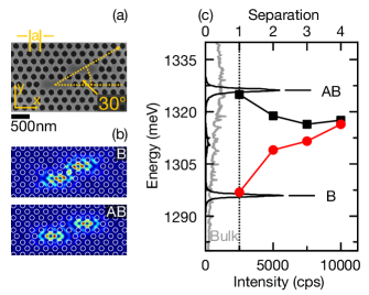
Figure 1: (a) SEM image of the PM formed by two L3 cavities. (b) $|E|^{2}$ extracted from FDTD simulations for the B (upper panel) and AB (lower panel) mode. The white circles indicate the air holes forming the PhC. (c) PL spectrum of the investigated PM (black curve), and QD emission from the unpatterned region of the sample (gray curve). The solid red dots and black squares indicate the simulated energetic position of the AB and B modes as a function of cavity separation.

III Results and Discussions

In figure 2 (a) we present a typical µ-PL spectrum recorded from the PM under pulsed non-resonant excitation. Again, we observe the emission of the B and AB modes as well as a sharp emission line attributed to a single QD at $1298.5\text{\,}\mathrm{meV}$, depicted in green, with a detuning of $\Delta E_{QD}=E_{QD}-E_{B}=$+2.8\text{\,}\mathrm{meV}$$ relative to the energy of the B mode ($E_{B}$). The respective relative energies of the B mode $E_{B}$ (red), the QD $E_{QD}$ (green) and the AB mode $E_{AB}$ (blue) are labeled on the figure. To demonstrate that spatially delocalized molecular-like modes are formed in the PM we excited the system at resonance at the AB mode energy. This allows us to directly pump the cavity mode and excite QDs that are located at positions close to the electric field antinodes within either of the two cavities Nomura et al. (2006); Kaniber et al. (2009). To do this, we tuned a single frequency laser across the emission energy of the AB mode from $1327.2\text{\,}\mathrm{meV}$ to $1324.0\text{\,}\mathrm{meV}$ in steps of $200\text{\,}\mathrm{\SIUnitSymbolMicro eV}$. Simultaneously, we detected emission spectra in the spectral vicinity of the B mode. Figure 2(b) shows the color-coded emission intensity as a function of the detection energy relative to the B mode, $\Delta E_{det}=E_{det}-E_{B}$, and the excitation laser energy $\Delta E_{exc}=E_{exc}-E_{B}$, for a pump power density of $94.5\text{\,}\mathrm{W}\text{\,}{\mathrm{cm}}^{-2}$. We observe two clear maxima at $\Delta E_{det}=$2.8\text{\,}\mathrm{meV}$$ and $\Delta E_{det}=$0\text{\,}\mathrm{meV}$$ when resonantly exciting via the AB mode ($\Delta E_{exc}=$29.3\text{\,}\mathrm{meV}$$) attributed to the QD and the B mode, respectively. The white line shows an emission spectrum for the resonance condition $\Delta E_{exc}=$29.3\text{\,}\mathrm{meV}$$ indicating that the QD and the bonding mode are simultaneously excited via the higher-energy AB mode. In figures 2(c) and (d), we compare horizontal cross-sections through the QD and B mode emission at $\Delta E_{det}=$2.8\text{\,}\mathrm{meV}$$ and $\Delta E_{det}=$0\text{\,}\mathrm{meV}$$, respectively. For both detection energies we simultaneously observe a clear maximum when resonantly exciting via AB. The dashed black lines show the PL spectrum of the AB mode for comparison. The observation of a shared absorption resonance for both the QD and B mode confirms that the two cavities are indeed coupled and that the QD is spatially coupled to one of the two cavities forming the PM.

After confirming the coupled character of the two cavities forming the PM, we present detailed investigations of the linear and non-linear optical properties of the PM coupled to the QD. Figure 3(a) shows typical emission spectra from the PM subject to non-resonant pulsed excitation at $1580\text{\,}\mathrm{meV}$ as the excitation power density is increased from $\sim 2\text{\,}\mathrm{W}\text{\,}{\mathrm{cm}}^{-2}$ to $>200\text{\,}\mathrm{W}\text{\,}{\mathrm{cm}}^{-2}$. As discussed already in the previous paragraph, we observe pronounced emission from B, AB and the QD. More strikingly, an additional emission feature, labeled W in figure 3(a), emerges for elevated excitation power densities. The unexpected W emission is energetically centered precisely between B and AB at $E_{M}=$1311\text{\,}\mathrm{meV}$\approx(E_{AB}+E_{B})/{2}$. In figure 3(b) we present the integrated peak intensities of B, AB, QD and W as a function of the excitation power density, plotted on a double logarithmic representation. The filled symbols label the excitation power densities selected for the spectra plotted in figure 3(a). The QD transition increases linearly with excitation power density, followed by saturation of the emission for excitation power densities above $P_{sat}^{QD}=$13\pm 2\text{\,}\mathrm{W}\text{\,}{\mathrm{cm}}^{-2}$$, as indicated by the dashed line in figure 3(b). The B mode also increases linearly with an exponent of $1.07\pm 0.02$, due to non-resonant feeding via QD ground states Laucht et al. (2010); Hohenester (2010); Winger et al. (2009). In contrast, we observe for the AB mode a clear superlinear increase in intensity of $1.65\pm 0.03$, most likely arising from its proximity to excited QD states. This attribution is supported by time-resolved measurements discussed in detail in figure 5(a). Both A and AB modes saturate at comparable power densities of $P_{sat}=$54\pm 4\text{\,}\mathrm{W}\text{\,}{\mathrm{cm}}^{-2}$$ highlighted with the dotted line in figure 3(b). For the unexpected W peak, we observe a super-linear exponent of $1.68\pm 0.03$, despite being at lower energy than expected for the QD excited states. Moreover, the W peak exhibits a similar saturation power density $P_{sat}=$54\pm 4\text{\,}\mathrm{W}\text{\,}{\mathrm{cm}}^{-2}$$ as the B and AB modes. This excitation power is $4.3\times$ higher than the saturation power $P_{sat}^{QD}$ observed for the QD.

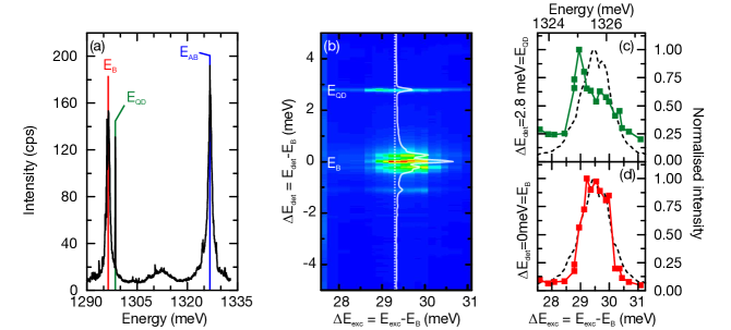
Figure 2: (a) PL emission spectrum of the PM under pulsed above band gap excitation. On the high energy side of the B mode the emission line of a QD, depicted in green, is observed with a detuning of $\Delta E_{QD}=$+2.8\text{\,}\mathrm{meV}$$. The according energies are labeled with B, QD, and AB. (b) Emission intensity as a function of excitation laser energy, whilst tuning the laser across the antibonding resonance. The white line shows an emission spectrum for the excitation energy marked by the white dotted line. (c) Emitted intensity at the QD energy at $\Delta E_{det}=$+2.8\text{\,}\mathrm{meV}$$ as a function of laser detuning. The dashed line shows PL emission of the AB mode subjected to non-resonant excitation for comparison. (d) Emitted intensity of the bonding mode at $\Delta E_{det}=$0\text{\,}\mathrm{meV}$$. The dashed line shows PL emission of the AB subjected to non-resonant excitation mode for comparison.

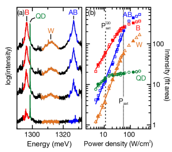
Figure 3: (a) PL intensity of the investigated PM plotted on an logarithmic scale when subjet to pulsed non-resonant excitation. (b) Extracted integrated intensities of B, AB, QD and W as a function of the pump power density, shown in double logarithmic representation. The excitation power densities for the plotted spectra in (a) are highlighted with filled symbols. the black dashed and dotted lines show the saturation power density of the QD $P_{sat}^{QD}$ and the common saturation power $P_{sat}$ of the B, AB and W peak, respectively. The solid lines represent power-law fits to the data points.

In order to shed light on the origin of the W peak, we present in the following temperature dependent PL measurements which enable us to clearly distinguish between the QD-excitonic or photonic character of the individual emission features. For the cavity modes, we expect a weak and approximately linear shift with increasing temperature, due to the change in the refractive index with increasing temperature Marple (1964). In contrast, the QD is expected to exhibit a significantly stronger shift determined by a Varshni type relation $E_{gap}(T)=E_{gap}(T=0)-(\alpha T^{2})/(T+\beta)$, where $\alpha$ and $\beta$ are dependent on the material. For GaAs $\alpha=8.871\times 10^{-4}$, $\beta=572$ Varshni (1967) and $E_{gap}(T=0)=$1521.6\text{\,}\mathrm{meV}$$ Sturge (1962); Thurmond (1975) and for InAs $\alpha=3.158\times 10^{-4}$, $\beta=93$ and $E_{gap}(T=0)=$426\text{\,}\mathrm{meV}$$ Varshni (1967); Dixon and Ellis (1961). In figure 4(a), we present PL spectra recorded from the cavity modes (black curves) and a magnified region around W (orange curves), as well as the QD emission (green curves) for three selected crystal temperatures, $13\text{\,}\mathrm{K}$, $40\text{\,}\mathrm{K}$ and $65\text{\,}\mathrm{K}$ and two excitation power densities; $99\text{\,}\mathrm{W}\text{\,}{\mathrm{cm}}^{-2}$ (black and orange curves) and $3.2\text{\,}\mathrm{W}\text{\,}{\mathrm{cm}}^{-2}$ (green curves), respectively. For both cavity modes and the QD we observe clear shifts to lower energy with increasing lattice temperature. However, the QD exhibits a higher shift rate. In figure 4(b) we present the extracted peak positions of the different emission lines whilst tuning the sample temperature from $13crystaltemperatures\text{\,}\mathrm{K}$ to $70\text{\,}\mathrm{K}$ in steps of $5\text{\,}\mathrm{K}$. For the QD, we obtain a clear non-linear shift of the emission with temperature, yielding an average shift rate of $113.6\text{\,}\mathrm{\SIUnitSymbolMicro eV}\text{\,}{\mathrm{K}}^{-1}$. As expected, the average shift rates for the cavities modes A and AB are $25.4\text{\,}\mathrm{\SIUnitSymbolMicro eV}\text{\,}{\mathrm{K}}^{-1}$ and $27.6\text{\,}\mathrm{\SIUnitSymbolMicro eV}\text{\,}{\mathrm{K}}^{-1}$, respectively, and thus a factor ${}\times 4.3$ smaller as compared to the QD. The pronounced difference in shift rates for QD and B leads to a clear resonance for a temperature of $T=$52\text{\,}\mathrm{K}$$. We observe that the W peak (orange) shows an average shift of $21.1\text{\,}\mathrm{\SIUnitSymbolMicro eV}\text{\,}{\mathrm{K}}^{-1}$, similar to B and AB and stays centered between both modes over the whole temperature range studied, as supported by the calculated center energy $E_{M}$ shown in gray in figure 4 (b). This demonstrates that the observed peak W is predominantly photonic-like and most likely does not arise from excitonic QD states.

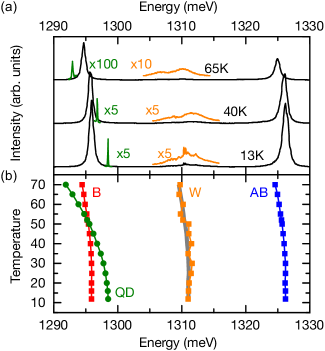
Figure 4: (a) PL emission of the PM for selected temperatures with an excitation power density of $99\text{\,}\mathrm{W}\text{\,}{\mathrm{cm}}^{-2}$ (black curves), magnified W peak (orange curves) and the QD emission under an excitation power of $3.2\text{\,}\mathrm{W}\text{\,}{\mathrm{cm}}^{-2}$ (green curves). (b) Peak energies of the B mode (red), the QD (green), the W (orange) and the AB mode (blue) as a function of crystal temperature. Grey shaded region marks the calculated center between B and AB.

Before identifying the nature of the unexpected W peak by comparing our results with a theoretical model, we continue to explore the decay dynamics of the coupled QD-PM using time-resolved spectroscopy. Measurements were performed as a function of emission energy ($$1290\text{\,}\mathrm{meV}$<E<$1327\text{\,}\mathrm{meV}$$) subject to non-resonant excitation at $1579\text{\,}\mathrm{meV}$ and a repetition frequency of $80\text{\,}\mathrm{MHz}$. We used a spectrometer as tunable $\Delta=$270\text{\,}\mathrm{\SIUnitSymbolMicro eV}$$ bandpass filter and recorded time transients using a time-correlated single-photon counting module Laucht et al. (2010). Figure 5(a) shows the complete detection energy- and time-resolved PL map. The white curve represents the time-integrated signal over all recorded times and resembles the typical PL spectra recorded with a CCD camera. We clearly observe the B and AB mode, as well as the QD that shows a $\sim 3$ times slower decay and, thus, is still visible in the time transient when the signal of the cavity modes have completely decayed. Both the B and AB modes exhibit fast decays, from which we extract exciton lifetimes of $\tau_{B}=$0.76\pm 0.1\text{\,}\mathrm{ns}$$ and $\tau_{AB}=$0.35\pm 0.1\text{\,}\mathrm{ns}$$, respectively. The shorter lifetime for the AB cavity mode is most likely caused by the spectral overlap with excited QD states Laucht et al. (2010). For the QD emission we observe a step-like increase in intensity as shown in figure 5(b), accompanied by a delayed onset of the luminescence decay. Moreover, a clear anti-correlation between the AB and the QD signal is observed; the AB mode has fully decayed prior to the QD decay. Both observations strongly suggest that the AB mode is predominantly fed from energetically higher excited multi-exciton states Laucht et al. (2011). In figure 5(b), we present selected decay transients of the B (red) and AB (blue) modes, the QD (green), as well as the W (orange) peak, as labeled in figure 5(a). The exciton lifetime from the delayed QD decay yields $\tau_{QD}=$2\pm 0.1\text{\,}\mathrm{ns}$$. The W peak, represented by the orange symbols in figure 5(b), shows a lifetime similar to the B and AB modes with $\tau_{M}=$0.75\pm 0.1\text{\,}\mathrm{ns}$$, supporting again our conclusion of the photonic-like origin of the W emission.

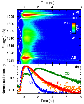
Figure 5: (a) Energy and time resolved µ-PL measurements of the PM. The color scale indicates the intensity of the recorded PL signal increasing from blue to red. The white line represents the time-integrated intensity over all collected times. (b) Selected decay transients for AB, B, QD and W under non-resonant excitation.

Finally, we performed CW resonant excitation of the W mode and power densities increasing from $290\text{\,}\mathrm{W}\text{\,}{\mathrm{cm}}^{-2}$ up to $8\text{\,}\mathrm{kW}\text{\,}{\mathrm{cm}}^{-2}$. The result, shown in figure 6(a), clearly shows emission from both B and AB. Although the excitation laser is tuned to lower energy than the AB mode, we detect significant emission from the higher energy AB mode (blue). The B mode can be directly excited via linear absorption of the excited states of the QD, since the laser is tuned to higher energy than the emission. In figure 6(b) we plot the PL intensity of AB as a function of the excitation power density. For low excitation power densities ($P<$1\text{\,}\mathrm{kW}\text{\,}{\mathrm{cm}}^{-2}$$) we observe a linear dependence of the emission from AB with an exponent of $1.04\pm 0.04$. However, for higher excitation power densities ($P>$2.5\text{\,}\mathrm{kW}\text{\,}{\mathrm{cm}}^{-2}$$) the emission becomes super-linear, with the yellow shaded region highlighting the difference between the linear and super-linear behavior. This indicates that the W mode is directly coupled to the B and AB modes, but there is a-priori no mechanism to account for this coupling. In the following, we will discuss how this arises from a coexistence of weak and strong coupling of the molecule.

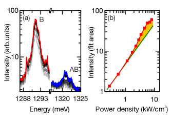
Figure 6: (a) µ-PL spectra detected from the PM under excitation with $10\text{\,}\mathrm{ps}$ pulses resonant to the W peak at $1311\text{\,}\mathrm{meV}$ for different optical pump powers. (b) PL intensity of AB as a function of excitation power density in double logarithmic representation depicted in red. The green line shows a linear power-law fitted to the first data points. The yellow area highlights the non linear fraction of the emission.

IV Identification of the anomalous peak

The observation of a triplet peak structure in solid-state in strong-coupling experiments Hennessy et al. (2007); Winger et al. (2008); Ota et al. (2009, 2018) has been a recurrent conundrum for theorists González-Tudela et al. (2010); Yamaguchi et al. (2009, 2012). Like in some other cases where a spectral triplet was observed when only a Rabi doublet was expected, our explanation relies on a mixture of weak and strong coupling. But instead of a mere incoherent superposition of the two regimes, that would be observed independently in separate time windows, our system involves an inextricable coexistence where both the weak and strong coupling occur simultaneously or at least during the smallest timescale of the system dynamics.

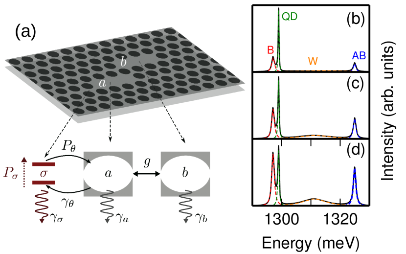
Figure 7: (a) Sketch of the model describing the system: a QD $\sigma$ coupled to cavity $a$, itself part of a photonic molecule with cavity $b$. Straight solid line is the Hamiltonian coherent coupling, curved solid lines is the Liouvillian coherent coupling that comes from the phonon-mediated transitions, dotted line is the incoherent pumping, wavy lines are the decay terms. (b-d) PM emission spectrum as a function of pumping (solid black lines) and its decomposition in terms of the various modes involved (colored lines). The couple of Rabi doublets from Eqs. (3) that can coexist gives rise to a triplet structure.

In our case, the key of the puzzle involves the strong, efficient and strongly asymmetric phonon-assisted coupling mechanism already characterized in such solid-state platforms Hohenester et al. (2009). The molecule finds itself in either one these two scenarios: with the QD that excited it in the first place, through a phonon-assisted process, now in its ground state, or, on the contrary, still in its excited state. Both situations are possible because there is a probabilistic aspect to both the excitation and emission of the various components so that the QD can be re-excited before the molecule gets de-excited. Nevertheless, this incoherent transfer of excitation is correlated, and this is a crucial element of the model. If the QD is de-excited, the molecule finds in the empty QD an efficient decay channel that brings it in weak-coupling. On the other hand, if the QD is still excited, the probability for the molecule to decay through this channel gets suppressed and it therefore retains its strong- coupling. We provide a simple theoretical model that produces this rich and unexpected phenomenology according to the mechanism we have just described. Unlike the model based on the multi-excitonic structure of the quantum dot Yamaguchi et al. (2009), our mechanism holds with a simple two-level system. The Hamiltonian itself is the simplest possible one to capture the key dynamics of our system: two cavities $a$ and $b$ coupled with a strength $g$ much larger than the coupling $g_{\sigma}$ of a QD $\sigma$ coupled to one cavity only. The Hamiltonian describing this situation reads

$$H=\omega_{a}a^{\dagger}a+\omega_{b}b^{\dagger}b+\omega_{\sigma}\sigma^{\dagger}\sigma+g(a^{\dagger}b+b^{\dagger}a)+g_{\sigma}(a^{\dagger}\sigma+\sigma^{\dagger}a)\,.$$ (1)

The dynamics is described with a master equation $i\partial_{t}\rho=[H,\rho]+\mathcal{L}\rho$ for the total density matrix $\rho$, where the Liouvillian $\mathcal{L}$ takes the form:

$$\mathcal{L}\equiv\gamma_{a}\mathcal{L}_{a}+\gamma_{b}\mathcal{L}_{b}+\gamma_{\sigma}\mathcal{L}_{\sigma}+P_{\sigma}\mathcal{L}_{\sigma}+P_{\theta}\mathcal{L}_{\sigma a^{\dagger}}+\gamma_{\theta}\mathcal{L}_{\sigma^{\dagger}a}\,,$$ (2)

where $\mathcal{L}_{c}\rho$ is the superoperator that is defined, for a generic operator $c$, as $c^{\dagger}c\rho+\rho c^{\dagger}c-2c\rho c^{\dagger}$. Equation (2) describes, respectively, the cavities $a$ and $b$ lifetime, the QD lifetime and rate of excitation and, crucially, an incoherent coupling mechanism between the QD and cavity $a$ leading to the excitation of the cavity by the QD (at rate $P_{\theta}$) or on the opposite to its de-excitation by transferring back the excitation to the QD (at rate $\gamma_{\theta}$). Importantly, however, this phonon-cavity coupling is correlated as arising from a simultaneous transfer of the excitation from the QD to the cavity, or vice-versa, as mediated by a phonon. These terms arise for instance from the phonon-mediated coupling studied experimentally and modelled theoretically by Majumdar et al. Majumdar et al. (2011) to account for this type of cavity feeding in microcavity QED. A sketch of this model is shown in figure 7(a). Note that the incoherent version of the QD-‘cavity $a$’ coupling allows different rates of excitation transfers, unlike the Hamiltonian case where the flow back and forth has the same rate $g_{\sigma}$. This is actually one of the important features of the model as the W peak is produced in conditions where $\gamma_{\theta}\gg P_{\theta}$. In fact, this condition is more important for producing a state-dependent configuration of the molecule emission than the saturable two-level character of the QD. The Diagonalisation of the master equation leads to two Rabi splittings for the QD–PM system:

$$R_{1} =\mathrm{Re}\sqrt{g^{2}-\left((\gamma_{a}-\gamma_{b})/4\right)^{2}}\,,$$ (3a)

$$R_{2} =\mathrm{Re}\sqrt{g^{2}-\left((\gamma_{a}+\gamma_{\theta}-\gamma_{b})/4\right)^{2}}\,.$$ (3b)

The first expression, Eq. (3a), is the standard Rabi splitting between the A and AB modes. The second expression, Eq. (3b), is similar but absorbs the phonon decay-rate $\gamma_{\theta}$ into the effective decay rate of the cavity that is coupled to the dot. The master equation shows that both of these Rabi rates enter the dynamics. This provides a quadruplet structure to the emission spectrum. However, the broadening corresponding to the weaker $R_{2}$-splitting is larger than that corresponding to $R_{1}$ and this makes difficult to resolve spectrally four peaks. Instead, one obtains features of a weakly-coupled system in the form of a broad single central peak. This is the structure we observe in the experiment as the W peak, although with hindsight, one could also recognize signs of a quadruplet for instance in figures 4(a) and 5(a). There, a doublet is apparent, although it is of imbalanced height, just as, however, the outer doublet (which could be due to a slight detuning or other variations from an ideal light-matter coupling scenario). At vanishing pumping, the phonon-mediated transfer is small and so is $\gamma_{\theta}$, making $R_{1}\approx R_{2}$ and there is only room for the expected, conventional strong-coupling picture of a Rabi doublet, as shown in figures 1(c) and 7(b). As the pumping is increased, the new decay channel that appeared can be so strong as to bring the molecule in the weak-coupling regime.

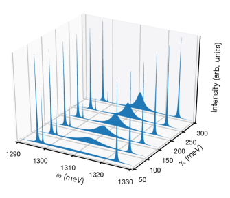
Figure 8: Calculated emission spectrum of the system as a function of $\gamma_{\theta}$, for the parameters $g=$14\text{\,}\mathrm{meV}$$, $g_{JC}=$0.14\text{\,}\mathrm{meV}$$, $\gamma_{a}=\gamma_{b}=$0.23\text{\,}\mathrm{meV}$$, $\gamma_{\sigma}=$0.001\text{\,}\mathrm{meV}$$, $E_{g}(0)=$1299.0\text{\,}\mathrm{meV}$$ and $\omega_{c}(T=0)=$1311\text{\,}\mathrm{meV}$$.

What is remarkable is that this does not destroy the Rabi doublet, however, since this decay channel is conditional on the state of the QD, which can saturate and stops perturbing the molecule’s dynamics, which recovers its strong-coupling. The necessity in the model of the correlated character for the excitation transfer between the QD and the PM as well as the existence of two Rabi splittings depending on the state of the QD suggest an analogy with phonon-sidebands, that are produced as the result of an optical transition affecting its surrounding matrix. Although phonons are also responsible in our case for making this scenario possible, the surrounding matrix itself is actually the QD and we have therefore a 0D counterpart of this phenomenon.

There is an excellent qualitative agreement between our simple minimalistic model and the experimental data, with all the notable features being reproduced. Figure 8, for instance, gives an overview of the spectral features as a function of increasing phonon-induced coupling $\gamma_{\theta}$, showing the neat transition from a conventional Rabi doublet for the PM in presence of a sharp and dominating QD line at low pumping, to a triplet with the added W line and a weakening contribution from the QD line at high pumping, as is observed experimentally (cf. figure 3).

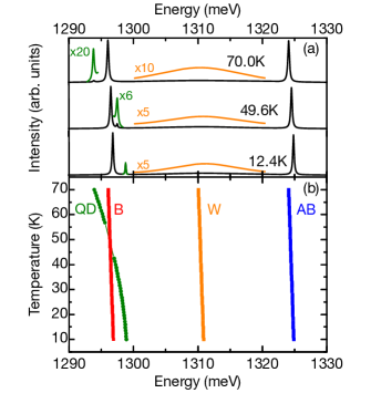
Figure 9: Emission spectrum of the photonic molecule system at different temperatures. Panel (a) $T=$70\text{\,}\mathrm{K}$$, $T=$49.6\text{\,}\mathrm{K}$$ and $T=$12.4\text{\,}\mathrm{K}$$. Additionally, panel (b) shows the center of the peaks as a function of the temperature for the parameters $g=$14\text{\,}\mathrm{meV}$$, $g_{\sigma}=$0.14\text{\,}\mathrm{meV}$$, $\gamma_{a}=\gamma_{b}=$0.23\text{\,}\mathrm{meV}$$, $\gamma_{\sigma}=$0.001\text{\,}\mathrm{meV}$$, $E_{g}(0)=$1299.0\text{\,}\mathrm{meV}$$, $\omega_{c}(T=0)=$1311\text{\,}\mathrm{meV}$$ and $P_{\sigma}=$0.08\text{\,}\mathrm{meV}$$.

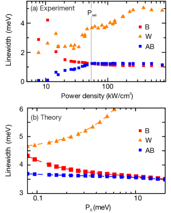
Figure 10: Linewidths as a function of the power density of the three emission peaks. The labels $B$ indicates bonding as red squares, $AB$ the anti-bonding as blue squares and $W$ central peak as orange triangles. The quantum dot is in resonance with the bonding mode. Experimental measurements are shown in panel (a), where the grey line highlights the saturation power $P_{sat}$ of the B and AB cavity modes. The numerical calculations based on our theoretical model are shown in panel (b) where the parameters used are $g=$14\text{\,}\mathrm{meV}$$, $g_{JC}=$0.14\text{\,}\mathrm{meV}$$, $\gamma_{a}=\gamma_{b}=$2.3\text{\,}\mathrm{meV}$$, $\gamma_{\sigma}=$0.6\text{\,}\mathrm{meV}$$, $P_{\theta}=$0.18\text{\,}\mathrm{meV}$$, $\gamma_{\theta}=$360\text{\,}\mathrm{meV}$$ and $T=$75\text{\,}\mathrm{K}$$.

Similarly, Fig. 9 shows how the temperature dependence matches with the experimental observation in Fig. 2, and in Fig. 10, the linewidths dependence are contrasted, with a good qualitative agreement. While there can be some quantitative differences, these are probably due to the fact that in the actual experiment, the key variables $P_{\sigma}$ and $\gamma_{\theta}$ are expected to be interconnected, while in the model, they are independent free parameters that we typically vary one at a time. In these conditions, it would be time consuming to aim for a fit of the data, that is also not guaranteed to be excellent since we have privileged a simple phenomenological model to capture the physics involved, rather than a more accurate but possibly also more confusing full semiconductor model that could provide such a quantitative agreement. In any case, the theoretical model unambiguously describes characteristic and distinctive features, and those are consistently observed in the experiment. The main consequences of this understanding of the anomalous W peak are thus that our system allows for a coexistence of weak and strong coupling, without either regime overtaking the other. This gives rise to a new regime of light-matter interactions with strong qualitative hallmarks, that have been observed thanks to the versatility and richer environment provided by a solid-state platform.

V Conclusions

We have studied the rich phenomenologies that occur in solid-state cQED experiments involving a QD coupled to a photonic molecule. We conducted a comprehensive experimental characterization of the structure using several techniques and in various regimes of excitation. At high pumping, we observed an unexpected feature in the form of an anomalous peak W that is energetically between the PM Rabi doublet. This peak, that bears all the features of a cavity mode, is explained by a simple phenomenological model of light-matter coupling between the QD and the PM that involves a type of coupling (phonon-mediated) that makes the molecule emit in two distinctive environments, that allow or on the opposite impede its strong-coupling. This results in a coexistence of both regimes, as is described theoretically by a simple phenomenological model that reduces the problem to its key ingredients. From this model, we can identify which elements are necessary from those that do not alter the phenomenological observation. For instance, the phonon-assisted Liouvillian coupling terms $\mathcal{L}_{\sigma^{\dagger}a}$ and $\mathcal{L}_{\sigma a^{\dagger}}$, describing incoherent, but correlated, transfers of excitation, are required, as mere rate equations do not reproduce this dynamical dependency of the molecule’s emission on the state of the QD, and only one regime is observed at a time (in which case a triplet would be observed if each regime could be established for long periods of time as compared to the system’s dynamics but short as compared to the integration time, as previously discussed in the literature Hennessy et al. (2007)). Our observations show how the richer and highly tunable geometries that are made possible by solid-state microcavity QED can give rise to new regimes of light-matter interactions that bring curious variations on otherwise familiar themes.

Acknowledgements:

We gratefully acknowledge financial support from the DFG via SFB-631, Teilprojekt B3 and the german excellence initiative via the Nanosystems Initiative Munich, the BMBF via Project No. 16KIS0110, part of the Q.com-Halbleiter consortium and the Ministry of Science and Education of the Russian Federation (RFMEFI61617X0085). S.E.-A. and H.V.-P. gratefully acknowledge funding by COLCIENCIAS project “Emisión en sistemas de Qubits Superconductores acoplados a la radiación. Código 110171249692, CT 293-2016, HERMES 31361”. S.E.-A. acknowledges support from the “Beca de Doctorados Nacionales de COLCIENCIAS 727”. E.A.G acknowledges financial support from the Vicerrectoría de Investigaciones, Universidad del Quindío.

References

- Arakawa et al. (2015) Y. Arakawa, J. Finley, R. Gross, F. Laussy, E. Solano, and J. Vuckovic, New J. Phys. 17, 010201 (2015).
- Haroche (2013) S. Haroche, Rev. Mod. Phys. 85, 1083 (2013).
- Kuruma et al. (2016) K. Kuruma, Y. Ota, M. Kakuda, D. Takamiya, S. Iwamoto, and Y. Arakawa, Appl. Phys. Lett. 109, 071110 (2016).
- Lodahl et al. (2015) P. Lodahl, S. Mahmoodian, and S. Stobbe, Reviews of Modern Physics 87, 347 (2015).
- O’Brien et al. (2009) J. L. O’Brien, A. Furusawa, and J. Vučković, Nature Photonics 3, 687 (2009).
- Soljačić and Joannopoulos (2004) M. Soljačić and J. D. Joannopoulos, Nature materials 3, 211 (2004).
- Englund et al. (2007) D. Englund, A. Faraon, I. Fushman, N. Stoltz, P. Petroff, and J. Vučković, Nature 450, 857 (2007).
- Fushman et al. (2008) I. Fushman, D. Englund, A. Faraon, N. Stoltz, P. Petroff, and J. Vučković, Science 320, 769 (2008).
- Englund et al. (2010) D. Englund, B. Shields, K. Rivoire, F. Hatami, J. Vuckovic, H. Park, and M. D. Lukin, Nano letters 10, 3922 (2010).
- Volz et al. (2012) T. Volz, A. Reinhard, M. Winger, A. Badolato, K. J. Hennessy, E. L. Hu, and A. Imamoğlu, Nature Photonics 6, 605 (2012).
- Englund et al. (2012) D. Englund, A. Majumdar, M. Bajcsy, A. Faraon, P. Petroff, and J. Vučković, Physical review letters 108, 093604 (2012).
- Choi et al. (2017) H. Choi, M. Heuck, and D. Englund, Phys. Rev. Lett. 118, 223605 (2017), URL doi:10.1103/PhysRevLett.118.223605.
- Bayer et al. (1998) M. Bayer, T. Gutbrod, J. Reithmaier, A. Forchel, T. Reinecke, P. Knipp, A. Dremin, and V. Kulakovskii, Physical review letters 81, 2582 (1998).
- Atlasov et al. (2008) K. A. Atlasov, K. F. Karlsson, A. Rudra, B. Dwir, and E. Kapon, Optics express 16, 16255 (2008).
- Dousse et al. (2010a) A. Dousse, J. Suffczyński, A. Beveratos, O. Krebs, A. Lemaître, I. Sagnes, J. Bloch, P. Voisin, and P. Senellart, Nature 466, 217 (2010a).
- Chalcraft et al. (2011) A. Chalcraft, S. Lam, B. Jones, D. Szymanski, R. Oulton, A. Thijssen, M. Skolnick, D. Whittaker, T. Krauss, and A. Fox, Optics express 19, 5670 (2011).
- Atlasov et al. (2011) K. A. Atlasov, A. Rudra, B. Dwir, and E. Kapon, Optics express 19, 2619 (2011).
- Majumdar et al. (2012) A. Majumdar, A. Rundquist, M. Bajcsy, and J. Vučković, Physical Review B 86, 045315 (2012).
- Cai et al. (2013) T. Cai, R. Bose, G. S. Solomon, and E. Waks, Applied Physics Letters 102, 141118 (2013).
- Haddadi et al. (2014) S. Haddadi, P. Hamel, G. Beaudoin, I. Sagnes, C. Sauvan, P. Lalanne, J. A. Levenson, and A. M. Yacomotti, 22, 12359 (2014), URL doi:10.1364/OE.22.012359.
- Kapfinger et al. (2015) S. Kapfinger, T. Reichert, S. Lichtmannecker, K. Müller, J. J. Finley, A. Wixforth, M. Kaniber, and H. J. Krenner, Nature communications 6 (2015).
- Du et al. (2016) H. Du, X. Zhang, G. Chen, J. Deng, F. S. Chau, and G. Zhou, Scientific Report 6, 24766 (2016), URL doi:10.1038/srep24766.
- Dousse et al. (2010b) A. Dousse, J. Suffczyński, O. Krebs, A. Beveratos, A. Lemaître, I. Sagnes, J. Bloch, P. Voisin, and P. Senellart, Applied Physics Letters 97, 081104 (2010b).
- Liew and Savona (2010) T. Liew and V. Savona, Physical review letters 104, 183601 (2010).
- Longo et al. (2010) P. Longo, P. Schmitteckert, and K. Busch, Physical review letters 104, 023602 (2010).
- Bose et al. (2014) R. Bose, T. Cai, K. R. Choudhury, G. S. Solomon, and E. Waks, Nature Photonics (2014).
- Hartmann et al. (2006) M. J. Hartmann, F. G. Brandao, and M. B. Plenio, Nature Physics 2, 849 (2006).
- Greentree et al. (2006) A. D. Greentree, C. Tahan, J. H. Cole, and L. C. Hollenberg, Nature Physics 2, 856 (2006).
- Houck et al. (2012) A. A. Houck, H. E. Türeci, and J. Koch, Nature Physics 8, 292 (2012).
- Rivoire et al. (2010) K. Rivoire, Z. Lin, F. Hatami, and J. Vuckovic, Appl. Phys. Lett 97, 043103 (2010).
- Rivoire et al. (2011) K. Rivoire, S. Buckley, and J. Vučković, Optics express 19, 22198 (2011).
- Armstrong et al. (1962) J. Armstrong, N. Bloembergen, J. Ducuing, and P. Pershan, Physical Review 127, 1918 (1962).
- Diederichs et al. (2006) C. Diederichs, J. Tignon, G. Dasbach, C. Ciuti, A. Lemaitre, J. Bloch, P. Roussignol, and C. Delalande, Nature 440, 904 (2006).
- Kammerer et al. (2001) C. Kammerer, G. Cassabois, C. Voisin, C. Delalande, P. Roussignol, and J. Gérard, Physical review letters 87, 207401 (2001).
- Xu et al. (2014) Q. Xu, C. Piermarocchi, Y. V. Pershin, G. Salamo, M. Xiao, X. Wang, and C.-K. Shih, Scientific reports 4 (2014).
- Akahane et al. (2003) Y. Akahane, M. Mochizuki, T. Asano, Y. Tanaka, and S. Noda, Applied Physics Letters 82, 1341 (2003).
- Nomura et al. (2006) M. Nomura, S. Iwamoto, T. Nakaoka, S. Ishida, and Y. Arakawa, Applied physics letters 88, 141108 (2006).
- Kaniber et al. (2009) M. Kaniber, A. Neumann, A. Laucht, M. Huck, M. Bichler, M. Amann, and J. Finley, New Journal of Physics 11, 013031 (2009).
- (39) Lumerical, https://www.lumerical.com/, [Online accessed: 26-January-2015], URL https://www.lumerical.com/.
- Laucht et al. (2010) A. Laucht, M. Kaniber, A. Mohtashami, N. Hauke, M. Bichler, and J. Finley, Physical Review B 81, 241302 (2010).
- Hohenester (2010) U. Hohenester, Physical Review B 81, 155303 (2010).
- Winger et al. (2009) M. Winger, T. Volz, G. Tarel, S. Portolan, A. Badolato, K. J. Hennessy, E. L. Hu, A. Beveratos, J. Finley, V. Savona, et al., Physical review letters 103, 207403 (2009).
- Marple (1964) D. Marple, Journal of Applied Physics 35, 1241 (1964).
- Varshni (1967) Y. Varshni, Physica 34, 149 (1967).
- Sturge (1962) M. D. Sturge, Physical Review 127, 768 (1962).
- Thurmond (1975) C. Thurmond, Journal of the Electrochemical Society 122, 1133 (1975).
- Dixon and Ellis (1961) J. R. Dixon and J. M. Ellis, Physical Review 123, 1560 (1961).
- Laucht et al. (2011) A. Laucht, N. Hauke, A. Neumann, T. Günthner, F. Hofbauer, A. Mohtashami, K. Müller, G. Böhm, M. Bichler, M.-C. Amann, et al., Journal of Applied Physics 109, 102404 (2011).
- Hennessy et al. (2007) K. Hennessy, A. Badolato, M. Winger, D. Gerace, M. Atature, S. Gulde, S. Fălt, E. L. Hu, and A. Ĭmamoḡlu, Nature 445, 896 (2007).
- Winger et al. (2008) M. Winger, A. Badolato, K. J. Hennessy, E. L. Hu, and A. Imamoğlu, Physical review letters 101, 226808 (2008).
- Ota et al. (2009) Y. Ota, N. Kumagai, S. Ohkouchi, M. Shirane, M. Nomura, S. Ishida, S. Iwamoto, S. Yorozu, and Y. Arakawa, Appl. Phys. Express 2, 122301 (2009).
- Ota et al. (2018) Y. Ota, D. Takamiya, R. Ohta, H. Takagi, N. Kumagai, S. Iwamoto, and Y. Arakawa, Appl. Phys. Lett. 112, 093101 (2018), URL doi:10.1063/1.5016615.
- González-Tudela et al. (2010) A. González-Tudela, E. del Valle, E. Cancellieri, C. Tejedor, D. Sanvitto, and F. P. Laussy, Opt. Express 18, 7002 (2010).
- Yamaguchi et al. (2009) M. Yamaguchi, T. Asano, K. Kojima, and S. Noda, Phys. Rev. B 80, 155326 (2009).
- Yamaguchi et al. (2012) M. Yamaguchi, T. Asano, and S. Noda, Rep. Prg. Phys. 75, 096401 (2012), URL doi:10.1088/0034-4885/75/9/096401.
- Hohenester et al. (2009) U. Hohenester, A. Laucht, M. Kaniber, N. Hauke, A. Neumann, A. Mohtashami, M. Seliger, M. Bichler, and J. J. Finley, Phys. Rev. B 80, 201311(R) (2009).
- Majumdar et al. (2011) A. Majumdar, E. D. Kim, Y. Gong, M. Bajcsy, and J. Vuckovic, Phys. Rev. B 84, 085309 (2011).