Sub-arcsecond Kinematic Structure of the Outflow in the Vicinity of the Protostar in L483

Abstract

The bipolar outflow associated with the Class 0 low-mass protostellar source (IRAS 18148–0440) in L483 has been studied in the CCH and CS line emission at 245 and 262 GHz, respectively. Sub-arcsecond resolution observations of these lines have been conducted with ALMA. Structures and kinematics of the outflow cavity wall are investigated in the CS line, and are analyzed by using a parabolic model of an outflow. We constrain the inclination angle of the outflow to be from 75° to 90°, i.e. the outflow is blowing almost perpendicular to the line of sight. Comparing the outflow parameters derived from the model analysis with those of other sources, we confirm that the opening angle of the outflow and the gas velocity on its cavity wall correlate with the dynamical timescale of the outflows. Moreover, a hint of a rotating motion of the outflow cavity wall is found. Although the rotation motion is marginal, the specific angular momentum of the gas on the outflow cavity wall is evaluated to be comparable to or twice that of the infalling-rotating envelope of L483.

1 Introduction

1.1 Outflows in Disk-Forming Regions

Disk formation around newly born solar-type protostars has extensively been studied both observationally and theoretically as one of central issues in astronomy and astrophysics. Especially, observational studies are rapidly being developed in the radio astronomy field, because high angular-resolution observations down to the disk-forming scale are becoming feasible with the advent of ALMA (e.g., Ohashi et al., 2014; Sakai et al., 2014a, b, 2016; Oya et al., 2014, 2015, 2016, 2017, 2018; Jørgensen et al., 2016; Takakuwa et al., 2017; Aso et al., 2017; Seifried et al., 2016; Yen et al., 2017; Alves et al., 2017; Lee et al., 2017a; Bianchi et al., 2017).

In these years, the detailed molecular distributions in the disk-forming regions have been revealed with ALMA in protostellar sources in their earliest evolutionary stages (Class 0–I), and it has been demonstrated that a gas motion of their infalling-rotating envelopes can be interpreted by the simple model assuming a ballistic motion (e.g., Sakai et al., 2014a, 2016; Oya et al., 2014, 2016; Maureira et al., 2017; Beuther et al., 2017; Alves et al., 2017; Lee et al., 2017a; Girart et al., 2017; van ’t Hoff et al., 2018; Csengeri et al., 2018). These results indicate that the gas falls beyond the centrifugal radius and even to a half of it (‘perihelion’). This position is called ‘centrifugal barrier’. More importantly, centrifugal barrier is suggested to be a boundary interfacing the infalling envelope with the rotationally-supported disk inside it; the gas motion of the disk/envelope system outside the centrifugal barrier can be regarded as the infaling-rotating motion, while that inside it can be as the Keplerian motion. These findings opened a new avenue to explore the transition from the envelope to the disk.

An important issue to be solved in the disk formation studies is how the specific angular momentum of the envelope gas is extracted to allow the gas to fall beyond the centrifugal barrier for disk formation. At the centrifugal barrier, the specific angular momentum of envelope gas is larger than that in the Keplerian disk by a factor of $\sqrt{2}$ (Appendix A). For the extraction mechanisms, outflow launching has been thought to play an important role (e.g. Shu et al., 1994a, b; Tomisaka, 2002; Machida et al., 2008; Hartmann, 2009; Machida & Hosokawa, 2013). In fact, rotating motion of outflows/jets has been reported (e.g., Zapata et al., 2010; Hirota et al., 2017; Lee et al., 2017b; Alves et al., 2017). To elucidate rotating motion of outflows/jets in terms of disk formation, observations of both an outflow/jet system and a disk/envelope system in the vicinity of a protostar is essential. We here characterize the molecular outflow of the low-mass protostellar source L483, for which the kinematic structure of the infalling-rotating envelope is already reported (Oya et al., 2017).

1.2 Target Source: L483

L483 is a dark cloud in Aquila Rift, whose distance from the Sun is 200 pc (Jørgensen et al., 2002; Rice et al., 2006). This cloud is associated with the infrared source IRAS 18148–0440, which is known to be a Class 0 protostar (Fuller et al., 1995; Chapman et al., 2013). The bolometric luminosity is 13 $L_{\odot}$, according to Shirley et al. (2000). The systemic velocity of this source is 5.5 km s^-1 (Hirota et al., 2009). Extensive studies have been reported for the large-scale outflow of this source (e.g. Fuller et al., 1995; Hatchell et al., 1999; Park et al., 2000; Tafalla et al., 2000; Jørgensen, 2004; Takakuwa et al., 2007; Velusamy et al., 2014; Leung et al., 2016). These studies reveal that the outflow blows along the east-west direction. The eastern component is red-shifted, while the western component is blue-shifted. Park et al. (2000) reported the position angle of the outflow axis in the plane of the sky to be 95° on the basis of the HCO⁺ ($J=1-0$) observation. Meanwhile, Chapman et al. (2013) reported it to be 105° on the basis of the shocked H₂ emission (Fuller et al., 1995). Fuller et al. (1995) claimed that the inclination angle of the outflow is about 50° with respect to our line of sight.

Recently, we reported the observation of this source in various molecular lines with ALMA (Oya et al., 2017). The CS ($J=5-4$; 245 GHz) emission was found to be mostly concentrated around the protostar, and its kinematic structure was interpreted as a combination model of the infalling-rotating envelope with the Keplerian disk. With the aid of the simulations assuming the ballistic motion (Oya et al., 2014), the radius of the centrifugal barrier, which approximately divides these two kinematic components, was estimated to be 100 au. Inside the centrifugal barrier, the emission lines of SO, CH₃OH, HCOOCH₃, and HNCO were detected. In addition to the centrally condensed components, an extended component is seen for the CS ($J=5-4$) and CCH ($N=3-2$) lines. They were found to trace the bipolar outflow components extended over scales of 1000 au from the protostar, according to the preliminary analysis (Oya et al., 2017). Characterization of the molecular outflow near its launching point is of potential importance in relation to the transition from the infalling-rotating envelope to the Keplerian disk. Here, we report detailed analyses of the outflow in this source.

2 Observations

The ALMA observations of L483 were carried out during its Cycle 2 operation (12 June 2014). The rotational lines of CCH, CS, and SO at 262.0, 244.9, and 261.8 GHz, respectively, were observed (ALMA Band 6). The line parameters are shown in Table 1. Other observational details were reported elsewhere (Oya et al., 2017).

We obtained images by employing the CLEAN procedure. The robustness parameter of the Brigg’s weighting was set to be 0.5. Self-calibration with the continuum data significantly improved the image quality. An image of the 1.2 mm continuum emission was prepared by averaging line-free channels. We subtracted the continuum component directly from the visibilities to prepare the line image. Table 1 lists the synthesized beam sizes for each line. We obtained the root-mean-square (rms) noise level of 0.13 mJy beam^-1 for the continuum image. The rms noise level of the CCH and CS line images is evaluated to be 8.2 and 7.6 mJy beam^-1, respectively, from nearby line-free channels, where the channel width is 61.030 kHz. The maximum recoverable size of these observations is 3$\farcs$3 for the CCH and CS lines, and 2$\farcs$0 for the SO line. The primary beam correction is not applied.

3 Distribution

Figure 1 shows the moment 0 images of the CCH, CS, and SO lines overlaid on the 1.2 mm dust continuum image. The synthesized beam size for the continuum image is $0\farcs 46\times 0\farcs 42$ (P.A. 11.​​°76). We determined the peak position of the continuum emission to be ($\alpha_{2000}$, $\delta_{2000}$) = (18^h17^m29$\fs$947, -04°39^′39$\farcs$55), by using the two-dimensional Gaussian fit. Figures 1(a), (b), and (d) were originally reported by Oya et al. (2017).

The CCH distribution is extended along the northwest-southeast direction. It seems to trace a part of the outflow components previously reported (e.g. Fuller et al., 1995; Hatchell et al., 1999; Park et al., 2000; Tafalla et al., 2000; Jørgensen, 2004; Takakuwa et al., 2007; Velusamy et al., 2014; Leung et al., 2016), although it is heavily resolved out. The CS distribution is also extended along the northwest-southeast direction. Although the intensity of the extended components appears faint in Figure 1(b) because of the wide velocity range for integration ($-2.5-13.5$ km s^-1), it is clearly seen in Figure 1(c) for the narrower velocity range ($3.0-5.5$ and $5.5-8.0$ km s^-1). Thus, CS also traces the outflow in spite of a heavy resolving-out problem. In addition to the outflow, a compact component around the continuum peak position is seen in the CS emission, which traces the disk/envelope system, as mentioned in Section 1.2 (Oya et al., 2017).

In contrast to the CCH and CS emission, the SO emission only traces the compact component around the continuum peak position in this source. Although the SO emission often traces the outflow and the outflow shocks (e.g. Bachiller & Pérez Gutiérrez, 1997), such a feature is not seen in this sources. The SO emission likely to trace the disk component near the protostar (Oya et al., 2017), although it has been reported to trace shocks near the disk edges in some other sources (e.g., Sakai et al., 2014a; Lee et al., 2016). The emitting region of the SO lines would thus be source-dependent.

Based on these molecular distributions, the CCH and CS emission seem to be appropriate for the outflow analysis. However, the hyperfine structure of the CCH line often makes its velocity structure complicated. In fact, the velocity offset of the hyperfine structure ($\sim 2.5$ km s^-1; see Table 1) is comparable to the velocity range of the outflow components in this source (see also Section 4). Therefore, we here focus on the outflow components traced by CS. In this paper, the position angle (P.A.) of the outflow is assumed to be 105° (Chapman et al., 2013), as shown in Figure 1(b).

4 Outflow Structure Traced by CS

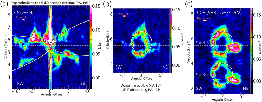
Figure 2: Position-velocity diagrams of CS (a, b) and CCH (c) along the outflow axis (a; P.A. 105°) and the line across the outflow (b, c; P.A. 15°) shown in Figure 1(b). The position axis in panels (b, c) is centered at the distance of 4″ from the protostellar position toward the southeastern direction. White lines represent the results of the parabolic outflow model, where the physical parameters are as follows; $i$ = 80°, $C$ = 0.0025 au^-1, and $v_{0}$ = 0.0015 km s^-1. In panel (c), the outflow model is prepared for each component of the two hyperfine components, whose separation is 2.54 km s^-1.

In Figure 1(c), red- and blue-shifted components are mutually overlapped with each other. This feature is also seen in the moment 1 map of the CS line (Figure 1e). It suggests that the outflow blows almost on the plane of the sky. Figure 2(a) depicts the position-velocity (PV) diagram (P.A. 105°) prepared along the outflow axis. The PV diagram is complicated at first glance, and each lobe of the bipolar outflow has both the blue- and red-shifted components. Figure 2(b) is the PV diagram along the line indicated by the arrow (P.A. 15°) in Figure 1(b), i.e. the line just across the southeastern outflow lobe. In this PV diagram, an elliptic feature is clearly seen. This feature can be confirmed also in the CCH emission (Figure 2c), although the two hyperfine components are nearly overlapped. Since the extended component is mostly resolved out in interferometric observations, this elliptic feature likely corresponds to the outflow cavity wall. Although both the red- and blue-shifted components are visible in Figure 2(b), the center velocity of the elliptic feature is slightly red-shifted from the systemic velocity (5.5 km s^-1; Hirota et al., 2009).

These observed features can be explained by the geometrical configuration shown in Figure 1(f); the outflow blows almost on the plane of the sky, and the center velocities of the northwestern and southeastern lobes are blue- and red-shifted, respectively. It should be noted that the geometrical configuration of the outflow, at least in the vicinity of the protostar, seems different from the previous report ($i\sim 50$°; Fuller et al., 1995) (see Section 5).

Such an outflow feature quite resembles that reported for the low-mass Class 0 source IRAS 15398–3359 (Oya et al., 2014; Bjerkeli et al., 2016). The kinematic structure of the outflow cavity wall of IRAS 15398–3359 is well explained by a parabolic model of an outflow (Oya et al., 2014). We therefore conduct a similar model analysis for L483. We employ the standard outflow model reported by Lee et al. (2000). Further details of the model are presented in Appendix B.

5 Model Analysis of the Outflow

In Figure 2, the outflow model result is overlaid in white lines on the PV diagrams of CS. It seems to well explain the observed feature of the CS line. In the model, a parabolic shape of the outflow cavity wall is assumed. Furthermore, the velocity on the cavity wall is assumed to be proportional to the distance to the protostar. The model parameters employed here are as follows; $i$ = 80°, $C$ = 0.0025 au^-1, and $v_{0}$ = 0.0015 km s^-1. (see Appendix B for their definitions.) This model is also shown in Figure 1(e). With the inclination angle less than 75° or larger than 90°, the kinematic structure cannot be reproduced by the model. Thus, the outflow axis almost on the plane of the sky is confirmed from this kinematical analysis. On the contrary, the inclination angle of this source has previously been reported to be 50° (Fuller et al., 1995). This inclination angle is evaluated from the asymmetric brightness of the two lobes in their near-infrared and submillimeter observations, and thus this discrepancy would come from the large uncertainty of the previous value. On the basis of this model analysis, Oya et al. (2017) employed the inclination angle of 80° for the kinematic analysis of the disk/envelope system.

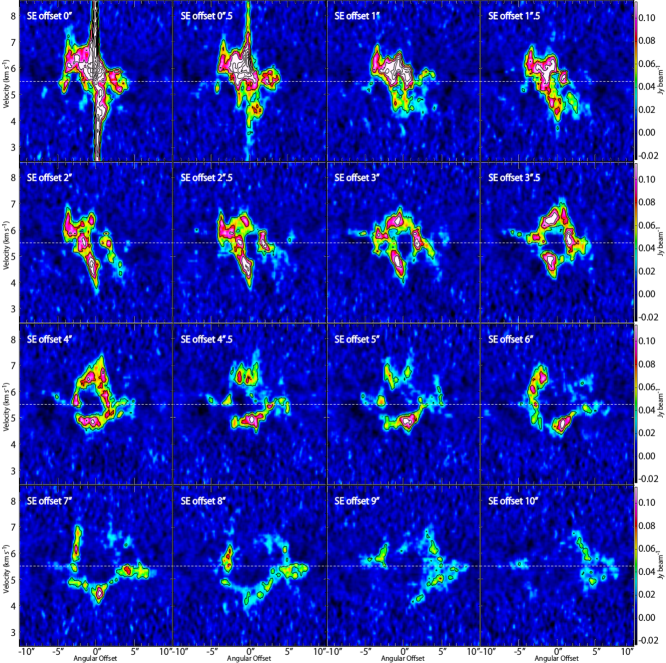
Figure 3: Position-velocity diagrams of CS ($J=5-4$) across the outflow axis. The position axes are along the position angle of 15°, which are perpendicular to the outflow axis (P.A. 105°). The origin of the position axes is on the outflow axis with offsets of the distance of ($0\arcsec-10\arcsec$) from the protostellar position toward the southeastern direction. The color map in the panel labeled as ‘SE offset 4″’ is the same as that in Figure 2(b). The contour levels for CS are every 5$\sigma$, where the rms noise level is 7.6 mJy beam^-1.

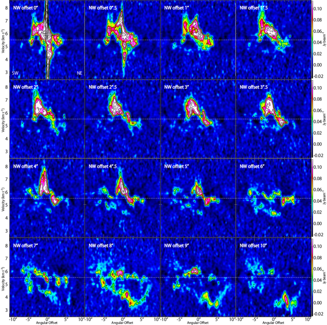
Figure 4: Position-velocity diagrams of CS ($J=5-4$) across the outflow axis. The position axes are along the position angle of 15°, which are perpendicular to the outflow axis (P.A. 105°). The origin of the position axes is on the outflow axis with offsets of the distance of ($0\arcsec-10\arcsec$) from the protostellar position toward the northwestern direction. The contour levels for CS are every 5$\sigma$, where the rms noise level is 7.6 mJy beam^-1.

Figure 3 shows the PV diagrams of CS ($J=5-4$), which are prepared for the position axes taken along the lines with the position angle of 15° (Figure 1b) with the offsets ($0\arcsec-10\arcsec$) from the protostellar position toward the southeastern direction (the red-shifted lobe). The origin of each position axis is taken on the outflow axis. Figure 4 is similar to Figure 3 except that the offset is taken toward the northwestern direction (the blue-shifted lobe). Although the diagrams seem to be heavily contaminated by the disk/envelope components in the panels with the offsets of ($0\arcsec-1\arcsec$) from the protostar, the elliptic feature of the outflow component (Figure 2b) can be confirmed in the panels with larger offsets. The radial size of the elliptic feature seems to be larger for a more distant position to the protostar. This feature indicates the expansion of the outflow cavity wall. The velocity centroid is slightly red- and blue-shifted in the southeastern and northwestern lobes, respectively, which supports the configuration shown in Figure 1(f). The PV diagrams of the two outflow lobes with the same offset from the protostar are not always similar to each other; for instance, the diagram with offset of 8″ in the blue-shifted lobe (Figure 4) shows a more extended feature than that in the red-shifted lobe (Figure 3). This asymmetry would be due to the difference of the ambient environment for the two lobes.

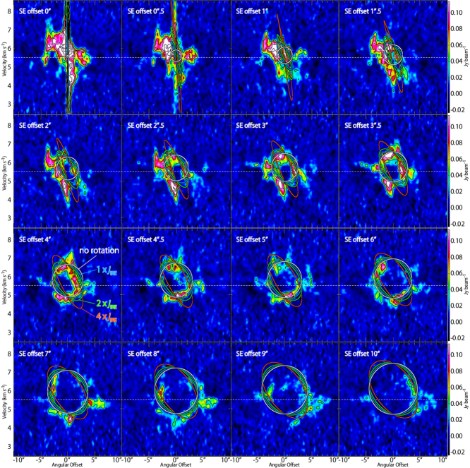
Figure 5: Position-velocity diagrams of CS ($J=5-4$) across the outflow axis. The color maps and the black contours are the same as those in Figure 3. Elliptic lines represent the results of the outflow model, where the physical parameters are as follows; $i$ = 80°, $C$ = 0.0025 au^-1, and $v_{0}$ = 0.0015 km s^-1. The specific angular momentumof the gas in the outflow is assumed to be $0$, $7.9\times 10^{-4}$, $15.8\times 10^{-4}$, and $31.6\times 10^{-4}$ km s^-1 pc for the white, blue, green, and red lines, respectively. The values for the latter three models correspond to once, twice, and four times of the specific angular momentum of the infalling-rotating envelope ($j_{\rm IRE}=7.9\times 10^{-4}$ km s^-1 pc). The specific angular momentum of the gas is assumed to be conserved in each outflow model.

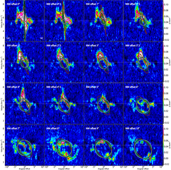
Figure 6: Position-velocity diagrams of CS ($J=5-4$) across the outflow axis. The color maps and the black contours are the same as those in Figure 4. Elliptic lines represent the results of the same outflow models shown in Figure 5.

The results of the above outflow model are superposed on these diagrams in white lines in Figures 5 and 6. In Figure 6, the observation shows excess of red-shifted velocity in the panels for the angular offset of less than 4$\farcs$5, which possibly comes from a local shock on the outflow cavity wall. Such a local shock is also seen in the outflow of IRAS 15398–3359 (Oya et al., 2014). Except for the above shock feature, the model results seem to reasonably explain the observed outflow components in all the panels.

By using the physical parameters estimated in the above analysis, the dynamical time scale ($t_{\rm dyn}$) of the outflow lobes is evaluated to be $(3\pm 1)\times 10^{3}$ yr with the relation: $t_{\rm dyn}=z/v_{z}=z_{0}/v_{0}$, where $z_{0}$ is 1 au (see Appendix B). Hatchell et al. (1999) previously reported model calculations with the dynamical time scale of $(2-6)\times 10^{3}$ yr for the CO ($J=4-3$, $2-1$) observations, while Yıldız et al. (2015) reported $(4.4-6.2)\times 10^{3}$ yr based on their CO ($J=6-5$, $3-2$) observations. On the other hand, Fuller et al. (1995) evaluated it to be $13\times 10^{3}$ yr based on the CO ($J=3-2$) observations. Since they assumed the inclination angle of 50°, the dynamical time scale is overestimated. It is recalculated to be $2\times 10^{3}$ yr by use of the inclination angle of 80° determined in our study. Thus, the dynamical time scales are almost consistent with one another, and its most plausible value would be a few $10^{3}$ yr. In particular, it should be stressed that the dynamical time scale derived from our observations at a 1000 au scale is consistent with the above previous reports based on the observations at larger scales (e.g. at $\sim 10000$ au scale; Yıldız et al., 2015). The outflow parameters for this source are summarized in Table 2.

6 Evolution of Outflows

6.1 Comparison with Other Sources

Oya et al. (2014, 2015) reported the kinematic structure of the outflow near the protostar for IRAS 15398–3359 and L1527 observed with ALMA as well as their envelope structure. The physical parameters for the outflow evaluated for these sources with the aid of the parabolic outflow model are summarized in Table 3.

Both IRAS 15398–3359 and L1527 have outflows blowing almost on the plane of the sky, as L483. However, their outflow shapes are quite different from each other. The outflow of IRAS 15398–3359 is well collimated, while that of L1527 shows a butterfly-feature. The L483 case seems in between. In the L1527 case, an offset of 1$\farcs$24 (170 au) between the launching points of blue-shifted and red-shifted lobes is assumed to account for the outflow structure, as reported by Tobin et al. (2008). In contrast, such an offset of the outflow launching points is not definitively seen in L483 as well as IRAS 15398–3359. This is probably because the envelope component would be contaminated with the outflow component near the protostar for the L483 and IRAS 15398–3359 cases. If such an offset is ignored for simplicity, the diversity of the opening angles of the outflow cavity is mainly translated to the variation of $C$ by an order of magnitude among these three sources.

In Table 3, the error ranges of the physical parameters for L483, IRAS 15398–3359, and L1527 are estimated on the basis of the simulations with a wide range of the parameters. The dynamical time scale of the outflow is evaluated to be $(1.9\pm 0.2)\times 10^{3}$ and $(6.5\pm 1.3)\times 10^{3}$ yr for IRAS 15398–3359 and L1527, respectively. These values are comparable to or different by a factor of a few from those reported based on larger scale observations (Table 3; Yıldız et al., 2015). It would be more appropriate to employ the dynamical time scales by Yıldız et al. (2015) rather than those derived from the outflow model. As for the L483 case, we employ the dynamical time scale estimated in our analysis ($t_{\rm dyn}=3\times 10^{3}$ yr), because it seems to be reliable, as discussed in Section 5.

6.2 Relation to Dynamical Ages

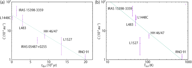
Figure 7: Relation between the curvature parameter ($C$) of an outflow, its dynamical time scale ($t_{\rm dyn}$; a), and bolometric temperature ($T_{\rm bol}$; b). The dynamical time scales for IRAS 15398–3359 and L1527 are the averaged value of the blue and red lobes. The green dashed lines represent the best-fit functions: $\log C=(-0.18\pm 0.03)\times(t_{\rm dyn}\times 10^{-3})+(-5.6\pm 0.3)$ and $\log C=(-1.1\pm 0.4)\times\log$ $T_{\rm bol}$$+(-2\pm 2)$ for (a) and (b), respectively. The correlation coefficients are $-0.95$ and $-0.85$ for (a) and (b), respectively, where the uniform weights are applied to all the sources.

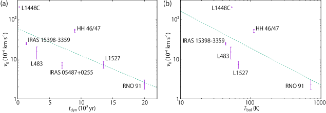
Figure 8: Relation between the velocity parameter ($v_{0}$) of an outflow, its dynamical time scale ($t_{\rm dyn}$; a), and its bolometric temperature ($T_{\rm bol}$; b). The dynamical time scales for IRAS 15398–3359 and L1527 are the averaged value of the blue and red lobes. The green dashed lines represent the best-fit functions: $\log v_{0}=(-0.15\pm 0.06)\times(t_{\rm dyn}\times 10^{-3})+(-5.2\pm 0.6)$ and $\log v_{0}=(-0.9\pm 0.6)\times\log$ $T_{\rm bol}$$+(-2\pm 3)$ for (a) and (b), respectively. The correlation coefficients are $-0.75$ and $-0.63$ for (a) and (b), respectively. where the uniform weights are applied to all the sources.

We compare the physical parameters of the outflow model ($C$ and $v_{0}$) and the dynamical time scale for the seven sources listed in Table 3. We also compare the model parameters and the bolometric temperature. Figures 7 and 8 show semi-log plots of $C$ and $v_{0}$ versus the dynamical time scale  and bolometric temperature, respectively. The plots with the dynamical time scale were previously reported by Oya et al. (2015) for the six sources except for L483. The outflow parameters for IRAS 05487$+$0255, RNO 91, L1448C, and HH 46/47 are converted to those in the units used for the other sources, as described in Appendix B (see also Oya et al., 2015). We excluded IRAS 05487$+$0255 in Figures 7 and 8, because the bolometric temperature is not available for this source.

As shown in Figures 7 and 8, the results for L483 seem to be consistent with those for the other sources. The dashed lines are obtained by linear fitting to the data under the assumption of equal weight. The correlation coefficients are $-0.95$, $-0.85$, $-0.75$, and $-0.63$ for the four plots. In spite of a small number of the sources, we can see a trend that both $C$ and $v_{0}$ decrease exponentially as an increasing dynamical time scale of the outflow and an increasing bolometric temperature.

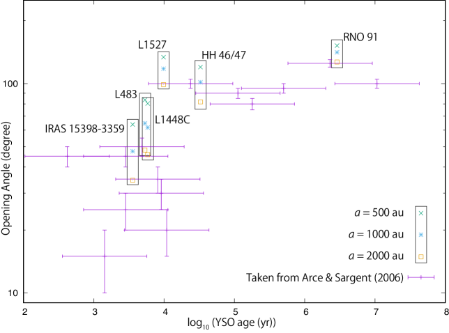
Figure 9: Relation between the opening angle of the outflow and the source age. The original plot was reported by Arce & Sargent (2006), from which three sources (L1527, L1448, and RNO91) are replaced by the results of this study. The sources listed in Table 3 are also shown in the plot, except for IRAS 05487$+$0255. The source age is obtained from the bolometric temperature by using the relation (Ladd et al., 1998): $\log(t_{\rm years})=[2.4\times\log(T_{\rm bol})-0.9]\pm 0.6$. For the samples taken from Arce & Sargent (2006), the errors for the source age come from this relation, while those for the opening angle are uniformly set to be 5°. For the other six sources, the opening angles are derived by adopting $a$ of 500, 1000, and 2000 au based on the outflow model analysis, which are approximate extents of the outflows (see Appendix B).

As discussed by Oya et al. (2015), the trend seen in Figure 7 well corresponds to the previous observational and theoretical results which report a relation between an opening angle of an outflow and a source age (e.g. Arce & Sargent, 2006; Shang et al., 2006; Seale & Looney, 2008; Offner et al., 2011; Machida & Hosokawa, 2013; Velusamy et al., 2014). Figure 9 shows the relation between the opening angle of the outflow and the source age. This plot was originally reported by Arce & Sargent (2006). In order to involve the sources listed in Table 3 in this plot, we calculated the opening angle of the outflow based on the model results (see Appendix B). These new samples are consistent with the trend reported by Arce & Sargent (2006).

Again, it should be stressed that we evaluate the outflow parameters in Table 3 from the full use of the geometrical and velocity structures of the outflow near the protostar considering the inclination angle, and provide quantitative supports of the above trends. Moreover, the ALMA results focused on narrow regions (at $\sim$ 1000 au scale; L483, IRAS 15398–3359, and L1527) are consistent with the other results based on the observations at larger scales. Thus, outflows can be characterized by focusing only on a small region around the protostar. This result further supports the idea that the outflow launching is mostly defined in the vicinity of the protostar.

7 Rotation Motion in the Outflow

In protostellar evolution, especially in disk formation, angular momentum of the gas is expected to play a crucial role. The infalling envelope gas needs to lose its angular momentum to fall becyond the centrifugal barrier for disk formation (Section 1.1). Outflow launching is thought to be a potential mechanism for the angular momentum extraction (e.g. Shu et al., 1994a, b; Tomisaka, 2002; Machida et al., 2008; Hartmann, 2009; Machida & Hosokawa, 2013). If this is the case, outflows would have a rotation motion. On the basis of this prediction, we examined the rotation motion of the outflow cavity wall in L1527 (Oya et al., 2015) without success because of the insufficient signal-to-noise (S/N) ratio of the available data. Here, we conduct such an analysis for L483, where the S/N ratio of the outflow image in the CS line is better than that in the L1527 case.

In Figures 1(c) and (e), we see a hint that there is a velocity gradient perpendicular to the outflow axis, although these maps possibly suffered by an asymmetric distribution of the gas or local shocks on the cavity wall. Moreover, when we carefully look at Figure 5, we may notice that the observed elliptic shape of the PV diagram tends to be elongated obliquely for the small offsets (1$\farcs$5–3″) in comparison with the simulation shown in white ellipses. A similar trend could be seen in Figure 6. Such a slant distortion of the expanding motion in the PV diagram suggests association of the rotation motion. Although the above trend is marginal, we examine the effect of the rotation of the outflow on the PV diagrams. The blue, green, and red elliptic lines in Figures 5 and 6 show the model results superposed on the PV diagrams of CS, where the rotation motion of the outflow is considered. The rotation velocity of the outflow cavity wall is simply calculated under assumption of the angular momentum conservation. In the model calculations, the specific angular momentum of the outflowing gas is assumed to be the same as that of the infalling-rotating envelope component ($j_{\rm IRE}$ = $7.9\times 10^{-4}$ km s^-1 pc; Oya et al., 2017) (blue ellipses in Figures 5 and 6), twice as much ($j=2\times$ $j_{\rm IRE}$; green ellipes), or four times as much ($j=4\times$ $j_{\rm IRE}$; red ellipses), as examples. When a larger specific angular momentum is assumed, a slant distortion of the elliptic feature in the PV diagram becomes more significant. Comparing the model results with the observations, we find a hint that the first and second models ($j=$ $j_{\rm IRE}$, $2\times$ $j_{\rm IRE}$; blue and green ellipses) would better reproduce the observations in the panels with the smaller offsets (e.g. an offset of $1\arcsec-4\arcsec$) than the model without rotation motion ($j=0$; white ellipses). The rotation motion seems to be overestimated in the third model ($j=4\times$ $j_{\rm IRE}$; red ellipses).

If the outflow is really extracting a substantial amount of the angular momentum from the envelope gas, the outflow should extract a larger specific angular momentum than that of the envelope. Suppose that a gas clump with the mass of $(m_{1}+m_{2})$ and the specific angular momentum of $j_{0}$ splits into two smaller gas clumps of the mass of $m_{1}$ and $m_{2}$ with the specific angular momentum of $j_{1}$ and $j_{2}$, respectively. Then, the conservation of angular momentum is expressed as:

$$(m_{1}+m_{2})\times j_{0} =m_{1}\times j_{1}+m_{2}\times j_{2},$$ (1)

If the small gas clump with the mass of $m_{1}$ falls toward the protostar because of angular momentum loss ($j_{1}<j_{0}$), the other small gas clump with the mass of $m_{2}$ is required to extract a larger specific angular momentum before the split ($j_{2}>j_{0}$). Thus, a better agreement for the second case ($j=2\times$ $j_{\rm IRE}$; green ellipes) seems reasonable. Moreover, the third ($j=4\times$ $j_{\rm IRE}$; red ellipses) case gives the upper limit to the specific angular momentum that the outflow is extracting. Nevertheless, it is difficult to evaluate the amount of the specific angular momentum and the total angular momentum extracted by the outflow accurately at the current stage.

As shown here, a change in the specific angular momentum by a factor of a few can affect the outflow feature in the PV diagrams. We can thus investigate the outflow rotation by looking at the kinematic structure much more carefully with better quality and higher angular resolution data, especially in the vicinity of its launching point, where the rotation motion is expected to be most prominent.

It should be noted that Hirota et al. (2017) recently reported a clear rotation motion of the outflow in the high-mass young stellar object candidate Orion Source I. They observed the outflow in the SiO line at an angular resolution of $\sim 0\farcs 1$ with ALMA, and detected rotation velocities of 17.9 and 7.0 km s^-1 at the distances of 24 and 76 au from the protostar, respectively. This rotation velocity is translated to the specific angular momentum of $2.1\times 10^{-3}$ and $2.6\times 10^{-3}$ km s^-1 pc, which is larger than that of L483 ($7.9\times 10^{-4}$ km s^-1 pc; Table 2).

8 Relation between the Envelope and the Outflow

8.1 Mass Rates of Outflow and Accretion

The outflow mass loss rate of L483 was reported to be $(5.4-14)\times 10^{-6}$ $M_{\odot}$ yr^-1 by Yıldız et al. (2015). Here, we compare this with the accretion rate. The averaged mass accretion rate ($\dot{M}_{\rm acc}$) can be estimated to be $5\times 10^{-5}$ $M_{\odot}$ yr^-1 from the dynamical time scale of $3\times 10^{3}$ yr (Section 5) and the protostellar mass ($M_{\rm star}$ = 0.15 $M_{\odot}$; Oya et al., 2017). The current mass accretion rate can also be derived from the bolometric luminosity by using the following equation (Palla & Stahler, 1991);

$$\dot{M}_{\rm acc} =\frac{L_{\rm bol}R_{\rm star}}{GM_{\rm star}},$$ (2)

where $R_{\rm star}$ denotes the protostar radius and $G$ the gravitational constant. Assuming $R_{\rm star}$ of 2.5 $R_{\odot}$ (e.g. Baraffe & Chabrier, 2010), $\dot{M}_{\rm acc}$ is calculated to be $6.9\times 10^{-6}$ $M_{\odot}$ yr^-1 by using the current bolometric luminosity. Compared with this value, the mass accretion rate derived from the dynamical time scale of the outflow may be larger than the outflow mass loss rate. Since the dynamical time scale is expected to give the lower limit for the source age, the mass accretion rate derived from it could be overestimated.

8.2 Is the Centrifugal Barrier the Launching Point of the Outflow?

Recent studies reveal that the gas motion in the envelope at a scale of a few 100 au from the protostar can be explained by the infalling-rotating envelope model (Sakai et al., 2014a, b, 2016; Oya et al., 2014, 2015, 2016, 2017). Moreover, the disk component seems to exist inside the centrifugal barrier, which can be traced by the H₂CS and H₂CO lines in IRAS 16293–2422 (Oya et al., 2016) and L1527 (Sakai et al., 2014b), respectively. Thus, the centrifugal barrier can be recognized as a boundary interfacing the infalling envelope with the disk component. However, the gas of the infalling envelope cannot fall into the disk beyond the centrifugal barrier, as long as its specific angular momentum is conserved, as mentioned before (Section 1.1). To extract the specific angular momentum of the envelope gas for disk formation and further growth of the protostar, the outflow launched around the centrifugal barrier could play an important role. A hint of the outflow rotation described in Section 7 may support this idea, if confirmed.

Alves et al. (2017) recently reported a support for this picture; the molecular outflow in BHB07-11 is clearly delineated with their ALMA observation, and it is found to be launched outside the disk, far from the protostellar position. We also found a similar feature in IRAS 16293–2422 Source B; the pole-on outflow lobes traced by the SiO line show a radial offset near the protostar, and their launching point seems to be near the centrifugal barrier traced by OCS and H₂CS ($r_{\rm CB}$ $\sim 40$ au; Oya et al., 2018). In L483, the SiO emission shows an intensity peak at the position apart from the protostar by 100 au, which is close to the position of the centrifugal barrier (Oya et al., 2017). Since SiO is known as a shock tracer (e.g. Mikami et al., 1992), the results for IRAS 16293–2422 Source B and L483 imply possible shocks caused by the collision of the outflowing gas with the infalling envelope gas near the centrifugal barrier.

Recently, Sakai et al. (2017) reported that the envelope gas in L1527 is accumulated in front of the centrifugal barrier, and that it has a substantial extension perpendicular to the mid-plane. It is likely that a part of the gas is escaping from the mid-plane. Sakai et al. (2017) suggested a possibility that this outflowing motion forms so-called ‘disk winds’ or ‘low-velocity molecular outflow’ launched at the centrifugal barrier. If so, one would expect a rotation motion of the outflow particularly near the centrifugal barrier.

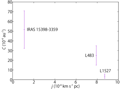
Figure 10: Plots of the curvature parameter ($C$) of the outflow against the specific angular momentum of the infalling-rotating envelope.

If the centrifugal barrier is responsible for the launch of the low-velocity outflow, there would be some relations between the radius of the centrifugal barrier and the outflow shape. To inspect its possibility, the outflow parameter $C$ is plotted against the specific angular momentum of the infalling-rotating envelope ($j$; Figure 10; Table 4). It shows a hint of decrease of $C$ as increase of $j$. However, the data points are limited, and hence, this possible relation has to be followed up in future works.

9 Summary

We analyzed the kinematic structure of the outflow in the Class 0 low-mass protostellar source L483 observed at a sub-arcsecond resolution with ALMA. The main results are summarized below:

1. The CCH and CS lines trace the bipolar outflow components extended at a 1000 au scale. On the other hand, the SO line, which is often regarded as the outflow tracer, does not trace the outflow components in this source.

2. Based on the distribution of the CS line and its kinematic structure, the geometrical configuration of the outflow is revealed. The outflow blows almost on the plane of the sky ($i\sim 80\arcdeg$), where the northwestern and southeastern lobes are blue- and red-shifted, respectively.

3. The parabolic model of the outflow well reproduces the geometrical and velocity structures of the outflow traced by the CS line. The physical parameters for the model are evaluated as follows: $C=$ 0.0025 au^-1, and $v_{0}=$ 0.0015 km s^-1.

4. The physical parameters for the parabolic outflow model are compared among seven protostellar sources. The parameters ($C$ and $v_{0}$) are further confirmed to decrease as the dynamical time scale of the outflow, which means that the opening angle of the outflow increases. A possible relation between the outflow parameters and the specific angular momentum of the infalling envelope is suggested, but it has to be examined by observations of more sources.

5. The rotation motion of the outflow is carefully inspected by using the outflow model taking account of the rotation. The PV diagrams seem to be better reproduced, if the specific angular momentum of the outflow cavity is a factor of a few of the infalling-rotating envelope. Thus, a hint of the rotation motion is found, although it is marginal.

Appendix A Specific Angular Momentum

Here, we consider the infalling-rotating envelope gas conserving the specific angular momentum (Sakai et al., 2014a; Oya et al., 2014). In this case, the specific angular momentum ($j$) is represented in terms of the mass of the protostar ($M$) and the radius of the centrifugal barrier ($r_{\rm CB}$) as:

$$j =\sqrt{2GMr_{\rm CB}},$$ (A1)

where $G$ denotes the gravitational constant. This is larger than the corresponding specific angular momentum for the Kepler motion at $r_{\rm CB}$ by a factor of $\sqrt{2}$:

$$j =\sqrt{GMr_{\rm CB}}.$$ (A2)

Oya et al. (2017) investigated the kinematic structure of the envelope gas of L483 with the aid of the infalling-rotating envelope model, and evaluated the protostellar mass ($M$) of 0.15 $M_{\odot}$ and the radius of the centrifugal barrier ($r_{\rm CB}$) of 100 au. Here, they assumed the inclination angle ($i$) to be 80° (0° for a face-on configuration) derived from the outflow analysis in this paper. With the above values, we evaluate the specific angular momentum of the gas to be $7.9\times 10^{-4}$ km s^-1 pc in the infalling-rotating envelope by using Eq. (A1).

Appendix B Parabolic Outflow Model

We analyze the outflow structure by using the standard model reported by (Lee et al., 2000). Although this is just a morphological model, it has widely been applied to outflows in low-mass and high-mass star forming regions (e.g. Arce et al., 2013; Beuther et al., 2004; Lumbreras & Zapata, 2014; Takahashi & Ho, 2012; Takahashi et al., 2013; Yeh et al., 2008; Zapata et al., 2014).

This model assumes a parabolic shape of the outflow cavity. It also assumes that the outflow velocity linearly increases as an increasing distance to the protostar. Then, the shape and the velocity of the outflow cavity wall are represented as:

$$z =CR^{2},\quad v_{R}=v_{0}\frac{R}{R_{0}},\quad v_{z}=v_{0}\frac{z}{z_{0}}.$$ (B1)

Here, we define the $z$-axis along the outflow, where the origin is taken at the protostar position. We set the normalization constant $z_{0}$ to be 1 au. On the other hand, the radial size of the outflow cavity is denoted by $R$, where the normalization constant $R_{0}$ is set to be 1 au. We fit this model to the observed PV diagrams, and determine the two free parameters, $C$ and $v_{0}$.

The outflow parameters for IRAS 05487$+$0255, RNO 91, L1448C, and HH 46/47 are originally reported in the unit of arcsecond (Lee et al., 2000; Hirano et al., 2010; Arce et al., 2013):

$$C_{\rm as} =CD,\quad v_{\rm as}=v_{0}D.$$ (B2)

Here, $D$ denotes the source distance. Hence, the coefficients of proportionality are converted to the values in the unit of au in Table 3.

The opening angle of the outflow ($\theta$) can be defined for a fixed distance of $a$. At the distance of $a$ along the outflow axis from the protostar (i.e. the length of the outflow), the radial size of the outflow is $\sqrt{a/C}$ in radius. Thus, the opening angle is expressed as:

$$\tan\frac{\theta}{2} =\frac{\sqrt{a/C}}{a}$$

$$=\frac{1}{\sqrt{aC}}.$$ (B3)

For instance, the opening angle of the outflow model for L483 is calculated to be 42°, 32°, and 24°, for $a$ of 500, 1000, and 2000 au, respectively. It should be noted that the opening angle decreases as increasing $a$, and thus the $a$ value should be fixed when comparing the opening angle among sources. Also, it should be stressed that the obtained opening angle is no longer under an influence of the inclination angle effect.

Table 1: Parameters of the Observed Lines

Molecule	Transition	Frequency (GHz)	$E_{u}$ (K)	$S\mu^{2}$ (Debye2)	$A_{ij}$ ($s^{-1}$)	Synthesized Beam
CS	$J=5-4$	244.9355565	35.3	19	2.98 $\times 10^{-4}$	$0\farcs 51\times 0\farcs 46$ (P.A. $2.\!\!\arcdeg 76$)
						$0\farcs 99\times 0\farcs 95$ (P.A. $-71.\!\!\arcdeg 95$)
SO	$J_{N}=6_{7}-5_{6}$	261.8437210	47.6	16	2.28 $\times 10^{-4}$	$0\farcs 46\times 0\farcs 42$ (P.A. 3.​​°09)
CCH	$N=3-2,J=7/2-5/2$
	$F=4-3$	262.0042600	25.1	2.3	5.32 $\times 10^{-5}$	$0\farcs 98\times 0\farcs 92$ (P.A. $-75.\!\!\arcdeg 93$)
	$F=3-2$	262.0064820	25.1	1.7	5.12 $\times 10^{-5}$	$0\farcs 98\times 0\farcs 92$ (P.A. $-75.\!\!\arcdeg 93$)

Table 2: Physical Parameters of L483

Outflow
Inclination Angle		80°
		(The NW lobe is blue-shifted.)
Position Angle		105°
Dynamic Timescale ($t_{\rm dyn}$)		$3\times 10^{3}$ yr
Outflow Mass Loss Rate ($\dot{M}_{\rm out}$)		$(5.4-14)\times 10^{-6}$ $M_{\odot}$ yr-1
Protostar/Envelope
Age		$<4.2\times 10^{3}$ yr
		(With an uncertainty of a factor of 3)
Central Mass ($M_{\rm star}$)		0.15 $M_{\odot}$
Bolometric Luminosity ($L_{\rm bol}$)		13 $L_{\odot}$
Bolometric Temperature ($T_{\rm bol}$)		$<56$ K
Accretion Rate ($\dot{M}_{\rm acc}$)	$(M_{\rm star}/t_{\rm dyn})$	$5\times 10^{-5}$ $M_{\odot}$ yr-1
	$(LR_{\rm star}/GM_{\rm star})$	$6.9\times 10^{-6}$ $M_{\odot}$ yr-1
Specific Angular Momentum ($j$)		$7.9^{+4}_{-3}\times 10^{-4}$ km s-1 pc

Table 3: Phsyical Parameters of Outflows

Source	Distance	$T_{\rm bol}$	$t_{\rm dyn}$	Inclination Angle	$C$	$v_{0}$
	(pc)	(K)	($10^{3}$ yr)	($\arcdeg$)	($10^{-4}$ au-1)	($10^{-4}$ km s-1)
L483	200	52	3	80 $\pm$ 5	$25\pm 10$	$15\pm 5$
IRAS 15398–3359	155	44	0.9 (northeast), 1.8 (southwest)	70 $\pm$ 10	52 $\pm$ 19	25 $\pm$ 2
L1527	137	67	20.6 (east), 6.5 (west)	85 $\pm$ 10	3.6 $\pm$ 2.2	7.3 $\pm$ 1.5
IRAS 05487$+$0255	460		$\sim$7	71 $\pm$ 3	4.8 $\pm$ 1.1	7.0 $\pm$ 1.1
RNO 91	160	715	$\sim$20	70 $\pm$ 4	1.3 $\pm$ 0.25	2.4 $\pm$ 0.6
L1448C	250	54	$\sim 0.24$	69	24, 32	200
HH 46/47	450	111.0	9	61 $\pm$ 1	6.7 $\pm$ 1.1	51 $\pm$ 4

Table 4: Physical Parameters of Envelopes

Source Name	Evolutionary	Inclination	Protostellar	Radius of	$j$
	Stage	Angle (°)	Mass ($M_{\odot}$)	the CB(au)	($10^{-4}$ km s-1 pc)
L483	Class 0	80	$0.15\pm 0.05$	$100^{+100}_{-70}$	$7.9^{+4}_{-3}$
IRAS 15398–3359	Class 0/I	70	$0.007^{+0.004}_{-0.003}$	40	$1.1\pm 0.3$
L1527	Class 0/I	85	$0.18\pm 0.05$	$100\pm 20$	$8.7\pm 1$

Figure 1: Integrated intensity maps of CCH ($N=3-2,J=7/2-5/2,F=4-3$ and $3-2$; a), CS ($J=5-4$; b, c), and SO ($J_{N}=6_{7}-5_{6}$; d). An outer taper of 1″ is applied for the CS data in panel (c). The velocity-shift range for integration is $\pm 8$ km s^-1 for CCH and CS (b), and $\pm 9$ km s^-1 for SO ($v_{\rm sys}=5.5$ km s^-1; Hirota et al., 2009). The CCH emission has the contribution from both the two hyperfine components (see Table 1). In panel (c) (CS), the velocity-shift range for integration is $(0-+2.5)$ and $(-2.5-0)$ km s^-1 for the red and blue contours, respectively. The outflow component is clearly seen in the maps for the narrower integration rarnges. The contour levels for the red and blue contours are every 5$\sigma$ from 3$\sigma$, where the rms noise level is 20 mJy beam^-1 km s^-1. The black contours represent the 1.2 mm continuum map, where the contour levels are 10, 20, 40, 80, and 160$\sigma$, where the rms noise level is 0.13 mJy beam^-1. The outflow axis is along the red arrow with a P.A. of 105° in panel (b). The PV diagram in Figure 2(b) is prepared along the red arrow with a P.A. of 15° in panel (b), which is centered at the position with an offset of 4″ to the southeast from the continuum peak along a P.A. of 105°. Panel (e) shows the velocity field (moment 1) map of CS with the velocity range for integration of $(-2.5-+2.5)$ km s^-1, on which the parabolic outflow model is superposed (see Section 5). Panel (f) shows a schematic illustration of the outflow, which blows almost on the plane of the sky.

References

- Arce & Sargent (2006) Arce, H. G., & Sargent, A. I. 2006, ApJ, 646, 1070
- Arce et al. (2013) Arce, H. G., Mardones, D., Corder, S. A., et al. 2013, ApJ, 774, 39
- Alves et al. (2017) Alves, F. O., Girart, J. M., Caselli, P., et al. 2017, A&A, 603, L3
- Aso et al. (2017) Aso, Y., Ohashi, N., Aikawa, Y., et al. 2017, ApJ, 849, 56
- Bachiller & Pérez Gutiérrez (1997) Bachiller, R., & Pérez Gutiérrez, M. 1997, ApJ, 487, L93
- Baraffe & Chabrier (2010) Baraffe, I., & Chabrier, G. 2010, A&A, 521, A44
- Beuther et al. (2004) Beuther, H., Schilke, P., & Gueth, F. 2004, ApJ, 608, 330
- Beuther et al. (2017) Beuther, H., Walsh, A. J., Johnston, K. G., et al. 2017, A&A, 603, A10
- Bianchi et al. (2017) Bianchi, E., Codella, C., Ceccarelli, C., et al. 2017, A&A, 606, L7
- Bjerkeli et al. (2016) Bjerkeli, P., Jørgensen, J. K., & Brinch, C. 2016, A&A, 587, A145
- Chapman et al. (2013) Chapman, N. L., Davidson, J. A., Goldsmith, P. F., et al. 2013, ApJ, 770, 151
- Chen et al. (1995) Chen, H., Myers, P. C., Ladd, E. F., & Wood, D. O. S. 1995, ApJ, 445, 377
- Csengeri et al. (2018) Csengeri, T., Bontemps, S., Wyrowski, F., et al. 2018, arXiv:1804.06482
- Fuller et al. (1995) Fuller, G. A., Lada, E. A., Masson, C. R., & Myers, P. C. 1995, ApJ, 453, 754
- Girart et al. (2017) Girart, J. M., Estalella, R., Fernández-López, M., et al. 2017, ApJ, 847, 58
- Green et al. (2013) Green, J. D., Evans, N. J., II, Jørgensen, J. K., et al. 2013, ApJ, 770, 123
- Hatchell et al. (1999) Hatchell, J., Fuller, G. A., & Ladd, E. F. 1999, A&A, 344, 687
- Hartmann (2009) Hartmann, L. 2009a, Astrophysics and Space Science Proceedings, 13, 23
- Hirano et al. (2010) Hirano, N., Ho, P. P. T., Liu, S.-Y., et al. 2010, ApJ, 717, 58
- Hirota et al. (2009) Hirota, T., Ohishi, M., & Yamamoto, S. 2009, ApJ, 699, 585
- Hirota et al. (2010) Hirota, T., Sakai, N., & Yamamoto, S. 2010, ApJ, 720, 1370
- Hirota et al. (2017) Hirota, T., Machida, M. N., Matsushita, Y., et al. 2017, Nature Astronomy, 1, 0146
- Jørgensen et al. (2002) Jørgensen, J. K., Schöier, F. L., & van Dishoeck, E. F. 2002, A&A, 389, 908
- Jørgensen (2004) Jørgensen, J. K. 2004, A&A, 424, 589
- Jørgensen et al. (2013) Jørgensen, J. K., Visser, R., Sakai, N., et al. 2013, ApJ, 779, L22
- Jørgensen et al. (2016) Jørgensen, J. K., van der Wiel, M. H. D., Coutens, A., et al. 2016, A&A, 595, A117
- Ladd et al. (1998) Ladd, E. F., Fuller, G. A., & Deane, J. R. 1998, ApJ, 495, 871
- Lee et al. (2000) Lee, C.-F., Mundy, L. G., Reipurth, B., Ostriker, E. C., & Stone, J. M. 2000, ApJ, 542, 925
- Lee et al. (2016) Lee, C.-F., Hwang, H.-C., & Li, Z.-Y. 2016, ApJ, 826, 213
- Lee et al. (2017a) Lee, C.-F., Li, Z.-Y., Ho, P. T. P., et al. 2017, ApJ, 843, 27
- Lee et al. (2017b) Lee, C.-F., Ho, P. T. P., Li, Z.-Y., et al. 2017, Nature Astronomy, 1, 0152
- Leung et al. (2016) Leung, G. Y. C., Lim, J., & Takakuwa, S. 2016, ApJ, 833, 55
- Lumbreras & Zapata (2014) Lumbreras, A. M., & Zapata, L. A. 2014, AJ, 147, 72
- Machida et al. (2008) Machida, M. N., Tomisaka, K., Matsumoto, T., & Inutsuka, S.-i. 2008, ApJ, 677, 327-347
- Machida & Hosokawa (2013) Machida, M. N., & Hosokawa, T. 2013, MNRAS, 431, 1719
- Maureira et al. (2017) Maureira, M. J., Arce, H. G., Dunham, M. M., et al. 2017, ApJ, 838, 60
- Mikami et al. (1992) Mikami, H., Umemoto, T., Yamamoto, S., & Saito, S. 1992, ApJ, 392, L87
- Müller et al. (2005) Müller, H. S. P., Schlöder, F., Stutzki, J., & Winnewisser, G. 2005, Journal of Molecular Structure, 742, 215
- Offner et al. (2011) Offner, S. S. R., Lee, E. J., Goodman, A. A., & Arce, H. 2011, ApJ, 743, 91
- Ohashi et al. (2014) Ohashi, N., Saigo, K., Aso, Y., et al. 2014, ApJ, 796, 131
- Okoda et al. (2018) Okoda, Y., Oya, Y., Sakai, N., et al. 2018, in prep.
- Oya et al. (2014) Oya, Y., Sakai, N., Sakai, T., et al. 2014, ApJ, 795, 152
- Oya et al. (2015) Oya, Y., Sakai, N., Lefloch, B., et al. 2015, ApJ, 812, 59
- Oya et al. (2016) Oya, Y., Sakai, N., López-Sepulcre, A., et al. 2016, ApJ, 824, 88
- Oya et al. (2017) Oya, Y., Sakai, N., López-Sepulcre, A., et al. 2017, ApJ, 837, 174
- Oya et al. (2018) Oya, Y., Sakai, N., Watanabe, Y., et al. 2018, ApJ, in press.
- Palla & Stahler (1991) Palla, F., & Stahler, S. W. 1991, ApJ, 375, 288
- Park et al. (2000) Park, Y.-S., Panis, J.-F., Ohashi, N., Choi, M., & Minh, Y. C. 2000, ApJ, 542, 344
- Rice et al. (2006) Rice, E. L., Prato, L., & McLean, I. S. 2006, ApJ, 647, 432
- Sakai et al. (2014a) Sakai, N., Sakai, T., Hirota, T., et al. 2014a, Nature, 507, 78
- Sakai et al. (2014b) Sakai, N., Oya, Y., Sakai, T., et al. 2014b, ApJ, 791, L38
- Sakai et al. (2016) Sakai, N., Oya, Y., López-Sepulcre, A., et al. 2016, ApJ, 820, L34
- Sakai et al. (2017) Sakai, N., Oya, Y., López-Sepulcre, A., et al. 2017, MNRAS, 467, L76
- Seale & Looney (2008) Seale, J. P., & Looney, L. W. 2008, ApJ, 675, 427-442
- Seifried et al. (2016) Seifried, D., Sánchez-Monge, Á., Walch, S., & Banerjee, R. 2016, MNRAS, 459, 1892
- Shang et al. (2006) Shang, H., Allen, A., Li, Z.-Y., et al. 2006, ApJ, 649, 845
- Shirley et al. (2000) Shirley, Y. L., Evans, N. J., II, Rawlings, J. M. C., & Gregersen, E. M. 2000, ApJS, 131, 249
- Shu et al. (1994a) Shu, F., Najita, J., Ostriker, E., et al. 1994a, ApJ, 429, 781
- Shu et al. (1994b) Shu, F. H., Najita, J., Ruden, S. P., & Lizano, S. 1994b, ApJ, 429, 797
- Tafalla et al. (2000) Tafalla, M., Myers, P. C., Mardones, D., & Bachiller, R. 2000, A&A, 359, 967
- Takakuwa et al. (2007) Takakuwa, S., Kamazaki, T., Saito, M., Yamaguchi, N., & Kohno, K. 2007, PASJ, 59, 1
- Takakuwa et al. (2017) Takakuwa, S., Saigo, K., Matsumoto, T., et al. 2017, ApJ, 837, 86
- Takahashi & Ho (2012) Takahashi, S., & Ho, P. T. P. 2012, ApJ, 745, L10
- Takahashi et al. (2013) Takahashi, S., Ohashi, N., & Bourke, T. L. 2013, ApJ, 774, 20
- Tobin et al. (2008) Tobin, J. J., Hartmann, L., Calvet, N., & D’Alessio, P. 2008, ApJ, 679, 1364-1384
- Tomisaka (2002) Tomisaka, K. 2002, ApJ, 575, 306
- van ’t Hoff et al. (2018) van ’t Hoff, M. L. R., Tobin, J. J., Harsono, D., & van Dishoeck, E. F. 2018, arXiv:1803.04515
- Velusamy et al. (2014) Velusamy, T., Langer, W. D., & Thompson, T. 2014, ApJ, 783, 6
- Yang et al. (2018) Yang, Y.-L., Green, J. D., Evans, N. J., II, et al. 2018, arXiv:1805.00957
- Yeh et al. (2008) Yeh, S. C. C., Hirano, N., Bourke, T. L., et al. 2008, ApJ, 675, 454-463
- Yen et al. (2017) Yen, H.-W., Koch, P. M., Takakuwa, S., et al. 2017, ApJ, 834, 178
- Yıldız et al. (2015) Yıldız, U. A., Kristensen, L. E., van Dishoeck, E. F., et al. 2015, A&A, 576, A109
- Zapata et al. (2010) Zapata, L. A., Schmid-Burgk, J., Muders, D., et al. 2010, A&A, 510, A2
- Zapata et al. (2014) Zapata, L. A., Arce, H. G., Brassfield, E., et al. 2014, MNRAS, 441, 3696