Online Optimal Task Offloading with One-Bit Feedback

Abstract

Task offloading is an emerging technology in fog-enabled networks. It allows users to transmit tasks to neighbor fog nodes so as to utilize the computing resources of the networks. In this paper, we investigate a stochastic task offloading model and propose a multi-armed bandit framework to formulate this model. We consider the fact that different helper nodes prefer different kinds of tasks. Further, we assume each helper node just feeds back one-bit information to the task node to indicate the level of happiness. The key challenge of this problem lies in the exploration-exploitation tradeoff. We thus implement a UCB-type algorithm to maximize the long-term happiness metric. Numerical simulations are given in the end of the paper to corroborate our strategy.

Index Terms—  Task offloading, fog computing, online learning, MAB.

1 Introduction

With the arriving of Internet of Things (IoT), 5G wireless systems, and the embedded artificial intelligence, more and more data processing capability is required in mobile devices [1]. To benefit from all the available computational resources, fog computing (or mobile edge computing) has been considered to be a potential solution to enable computation-intensive and latency-critical applications at the battery-empowered mobile devices [2].

Fog computing promises dramatic reduction in latency and mobile energy consumption by offloading computation tasks [3]. Recently, many works have been carried out addressing the task offloading in fog computing [9, 8, 7, 6, 5, 4]. Among these works, some considered the energy issues and formulated the task offloading as deterministic optimization problems [5, 4]. Considering the real-time states of users and servers, the task offloading problem is a typical stochastic optimization problem. To make this problem tractable, in [9, 8, 7, 6], the Lyapunov optimization method was applied to transform the challenging stochastic optimization problem to a sequential decision problem.

Note that all the above literatures assumed perfect knowledge about the system parameters, e.g. the precise relationship among latency, energy consumption, and computational resources. However, in practice, the models may be too complicated to be modeled accurately and it is difficult to learn all the system parameters. For example, the communication delay and the computation delay were modeled as bandit feedbacks in [10], which were only revealed for the nodes that were queried. Without assuming particular system models and without perfect knowledge about the system parameters, the tradeoff between learning the system and pursuing the empirically best offloading strategy was investigated under the bandit model in [11]. The exploration versus exploitation tradeoff in [11] was addressed based on the multi-armed bandit (MAB) framework, which has been extensively studied in statistics [13, 14, 12].

In reality, it is hard to know the exact feedback rules of different fog nodes. This reality motivates us to find one unified and analytical model involving several features to approximate the behavior of fog nodes, e.g. whether they feel optimistic about the incoming task or not. Additionally, it is unnecessary to estimate all the parameters corresponding to every fog node since we just want to get optimistic feedbacks after offloading each task. Clearly, there exists a tradeoff between exploiting the empirically best node as often as possible and exploring other nodes to find more profitable actions. In this paper, we model the overall performance of offloading each task as one bit. This one-bit information is fed back to the task node after completing the task. The value of the feedback bit is modeled as a random variable and is related to some particular features of the task and the node processing the task. We endeavor to make online decisions to maximize the long-term performance of task offloading with these probabilistic feedbacks. Our main contributions are summarized as follows. First, we apply a bandit learning method to approximate the behavior of the concerned fog nodes and model the node uncertainty with a logit model, which is more practical than the previous ones, e.g. [4, 5, 6, 7]. Second, we extend the algorithm proposed in [15] to make it suitable to learn the feature weights of different fog nodes. We further analyze our proposed algorithm and establish the corresponding performance guarantee for our extension.

The rest of this paper is organized as follows. Section 2 introduces the system model and assumptions. Section 3 describes our algorithm and the related performance guarantees. Numerical results are provided in section 5 and Section 6 concludes the paper.

Notations: Notations $\bm{A}^{\top}$, $|\mathcal{A}|$, $\|\bm{x}\|_{A}^{2}$, $\Pr[A]$, and $\mathbb{E}[A]$ stand for the matrix transpose, the cardinality of the set $\mathcal{A}$, the norm with respect to $\bm{A}$, i.e. $\bm{x}^{\top}\bm{A}\bm{x}$ for a positive definite matrix $\bm{A}\in\mathbb{R}^{d\times d}$, the probability of event $A$, and the expectation of a random variable $A$. Indicator function $\mathds{1}\{\cdot\}$ takes the value of $1$ ($0$) when the specified condition is met (otherwise).

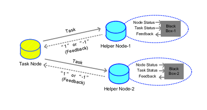
Fig. 1: A task offloading example. The task node offloads a task to a helper node and immediately receives a one-bit feedback representing “happy” or “unhappy”. The feedback is determined jointly by the node status and the task details.

2 System Model

We consider the task offloading problem in a network including $K$ fog nodes, i.e. one task node and $(K-1)$ helper nodes. See Fig. 1 for an example. Define the set of fog nodes as

$$\mathcal{I}:=\{\underbrace{1,2,\cdots,K-1}_{\rm helper~{}nodes},\underbrace{K}_{\rm task~{}node}\}.\vspace{-2mm}$$ (1)

In each time slot, the task node generates one task and intelligently chooses one fog node to offload this task. The helper nodes can also generate tasks occasionally. In this paper, we focus on the offloading decisions at the task node. We assume the tasks generated at the helper nodes are processed locally. Further, we assume all the incoming tasks at each node are cached and executed in a first-input first-output (FIFO) fashion.

In time slot-$t$, the task node offloads a task to a particular node-$I_{t}$ and receives a one-bit feedback $y_{I_{t}}^{(t)}$. This one-bit feedback $y_{I_{t}}^{(t)}$ indicates whether the helper node feels optimistic about the current task. Without loss of generality, we use $y_{I_{t}}^{(t)}=1\ (-1)$ to denote the node is happy (unhappy). In this paper, we assume the feedback is delivered immediately after receiving the offloaded task. As shown in Fig. 1, the feedback is determined jointly by the task details and the node status. To represent all the factors affecting the feedback $y_{i}^{(t)}$ from node-$i$, we combine them into a feature vector $\bm{x}_{i}^{(t)}$, whose elements is a series of hypothetical features to depict the model. The elements may include some real attributes, e.g. queue length, data length, task complexity, central processing unit (CPU) frequency, channel quality information (CQI). In general cases, however, the features have no specific meaning. Each element in $\bm{x}_{i}^{(t)}$ is normalized such that $\|\bm{x}_{i}^{(t)}\|_{2}\leq 1$. Note that different kinds of computing nodes certainly have different preferences over various tasks, which can be reflected by applying different weights to the features. Specifically, we can employ one weight vector $\bm{w}_{i}$ and each element quantifies the weight associated with the corresponding feature in $\bm{x}_{i}^{(t)}$. Similar to $\bm{x}_{i}^{(t)}$, we also normalize $\bm{w}_{i}$ such that $\|\bm{w}_{i}\|_{2}\leq 1$.

Note that it is hard to know the exact feedback rules of different fog nodes. In this paper, we assume each node exploits the logit model, a commonly used binary classifier [15], to evaluate the incoming tasks. Accordingly, the probability of feeding back $y_{i}^{(t)}=1$ or $y_{i}^{(t)}=-1$ is given by

$$\Pr\left[y_{i}^{(t)}=\pm 1|\bm{x}_{i}^{(t)}\right]=\frac{1}{1+\exp\left(-y_{i}^{(t)}\bm{w}_{i}^{\top}\bm{x}_{i}^{(t)}\right)},\vspace{-1mm}$$ (2)

where the pair $(\bm{x}_{i}^{(t)},\bm{w}_{i})$ is chosen from the following set

$$\mathcal{D}_{t}:=\{(\bm{x}_{i}^{(t)},\bm{w}_{i}),\forall i\in\mathcal{I}\}.$$ (3)

3 Problem Formulation

Our goal is to maximize the long-term happiness metric. Consider a time range $\mathcal{T}:=\{1,2,\cdots,T\}$. The maximization of the long-term happiness metric can be formulated as follows.

$$\begin{split}\underset{\{I_{t}\}}{\rm maximize}\quad&\underset{T\rightarrow\infty}{\rm lim}\ \frac{1}{T}\sum_{t\in\mathcal{T}}y_{I_{t}}^{(t)}\\ {\rm subject\ to}\quad&(\ref{Eq:FeedbackProb}),\ {I_{t}}\in\mathcal{I},\forall t\in\mathcal{T}.\end{split}$$ (4)

There are two difficulties in (4). First, the weight vector $\bm{w}_{i}^{(t)}$ is unknown to the task node. Furthermore, the offloading decision is made at the beginning of each time slot. Thus it is necessary to learn the weight vectors along with making the task offloading decisions. To deal with the latter one, we turn to solve the following problem as an alternative.

$$\begin{split}\underset{I_{t}}{\rm maximize}\quad&\mathbb{E}[y_{I_{t}}^{(t)}]\\ {\rm subject\ to}\quad&(\ref{Eq:FeedbackProb}),\ {I_{t}}\in\mathcal{I}.\end{split}$$ (5)

Although the above problem is not exactly the same as the original one in (4), it is one common approach and was adopted in [7, 8, 9, 11]. Meanwhile, under the stochastic framework [14], it is more natural to focus on the expectation, i.e. $\mathbb{E}[y_{I_{t}}^{(t)}]$. Note the expected happiness metric of each arm has to be estimated based on the historical feedback. There is thus an exploration-exploitation tradeoff in (5). On the one hand, the task node tends to choose the best node according to the historical information. On the other hand, trying offloading to unfamiliar nodes may bring task node extra rewards. Plenty of works have been done to deal with this kind of exploration-exploitation tradeoff problem under the MAB framework [11, 12, 13, 14, 15]. In the rest of the paper, we also address this tradeoff through the bandit methods.

4 Online task offloading

4.1 Task Offloading with One-bit Feedback

This exploration-exploitation tradeoff can be solved with a stationary multi-armed bandit (MAB) model, where each node can be viewed as one arm. Offloading one task is like testing one arm and the task node makes decisions according to all the feedbacks it has received. Given the first $T$ observations of the feedbacks, i.e. $y_{I_{t}}^{(t)},t=1,2,\cdots,T$, the weight vector of each fog node can be approximated by its maximum likelihood estimate as follows.

$$\bar{\bm{w}}_{i}^{(T)}=\arg\max_{\|\bm{w}\|\leq 1}\frac{1}{T}\sum_{t=1}^{T}f_{i}^{(t)}(\bm{w}),\forall i\in\mathcal{I},$$ (6)

where the log likelihood function is defined based on (2),

$$f_{i}^{(t)}(\bm{w})=-\log\left(1+\exp(-y^{(t)}_{i}{\bm{w}}^{\top}{\bm{x}_{i}})\right)\mathds{1}\{I_{t}=i\}.$$ (7)

Clearly, this approach needs to optimize over all the historical feedbacks, which is not scalable. To admits online updating, we refer to [15] and propose an approximate sequential MLE solution as

$$\begin{split}\bar{\bm{w}}_{i}^{(t+1)}&={\arg\max_{\|\bm{w}\|_{2}\leq 1}}-\frac{\|\bm{w}-\bar{\bm{w}}_{i}^{(t)}\|_{\bm{Z}_{i}^{(t)}}}{2}\\ &+(\bm{w}-\bar{\bm{w}}_{i}^{(t)})^{\top}\nabla f_{i}^{(t)}(\bar{\bm{w}}_{i}^{(t)})\mathds{1}\{I_{t}=i\},\end{split}$$ (8)

where

$$\bm{Z}_{i}^{(t+1)}=\bm{Z}_{i}^{(t)}+\frac{\beta}{2}{\bm{x}}_{i}^{(t)}({\bm{x}}_{i}^{(t)})^{\top}\mathds{1}\{I_{t}=i\}.$$ (9)

The term $\|\bm{w}-\bar{\bm{w}}_{i}^{(t)}\|_{\bm{Z}_{i}^{(t)}}$ in (8) is an exploration bonus. Specifically, if one fog node is explored deficiently, the restriction given by $\bm{Z}_{i}^{(t)}$ on the exploration bonus term is relatively loose. Thus the wider range of exploration of this node is more recommended.

As indicated in (5), our goal is to maximize the expectation of instantaneous happiness metric, which is positively correlated to the probability of $y_{I_{t}}^{(t)}=1$. Additionally, the metric is positively correlated to $\bm{w}_{i}^{\top}\bm{x}_{i}$ as well. In time slot-$t$, the task node then chooses one fog node to offload based on the feature $\bm{x}_{i}^{(t)}$ by solving the following optimization problem:

$$({\bm{x}}_{I_{t}}^{(t)},\hat{\bm{w}}_{I_{t}})=\arg\max_{(\bm{x},\bm{w})\in\bar{\mathcal{D}}_{t}}\bm{w}^{\top}\bm{x}.\vspace{-2mm}$$ (10)

Note $\hat{\bm{w}}_{I_{t}}$ is just a temporal variable that does not engage in the updates of any variables. Essentially, we are only interested in the index of the node, i.e. $I_{t}$. The domain $\bar{\mathcal{D}}_{t}$ is defined as

$$\bar{\mathcal{D}}_{t}=\bigcup_{i\in\mathcal{I}}\{(\bm{x},\bm{w})|\bm{x}=\bm{x}_{i}^{(t)},\bm{w}\in\mathcal{W}_{i}^{(t)}\},$$ (11)

and $\mathcal{W}_{i}^{(t)}$ denotes the feasible region of the estimated weights, which is a ball centered at $\bar{\bm{w}}_{i}^{(t)}$. Specifically, the ball is characterized as

$$\mathcal{W}_{i}^{(t)}:=\{\bm{w}|\|\bar{\bm{w}}_{i}^{(t)}-{\bm{w}}\|_{{\bm{Z}}^{(t)}_{i}}^{2}\leq{\gamma^{(t)}_{i}}\}.$$ (12)

The benefit of the exploration will be further explained in section 4.2. Note ${\gamma^{(t)}_{i}}$ is an important parameter, the value of which determines the performance of our proposed algorithm. Details about ${\gamma^{(t)}_{i}}$ and the corresponding theoretical guarantees will be discussed later in Section 4.2. Based on the feasible region of $\hat{\bm{w}}_{I_{t}}$ defined in (12), we can identify the node index $I_{t}$ in (10) as follows.

$$\begin{split}{I_{t}}&=\arg\max_{i\in\mathcal{I}}\ \left(\max_{\|\bar{\bm{w}}_{i}^{(t)}-{\bm{w}}\|_{{\bm{Z}}^{(t)}_{i}}^{2}\leq{\gamma^{(t)}_{i}}}\bm{w}^{\top}\bm{x}_{i}^{(t)}\right)\\ &=\arg\max_{i\in\mathcal{I}}\ \left((\bar{\bm{w}}_{i}^{(t)})^{\top}\bm{x}_{i}^{(t)}-\min_{\|\bm{z}\|_{2}^{2}\leq{\gamma^{(t)}_{i}}}[(\sqrt{{\bm{Z}}^{(t)}_{i}})^{-1}{\bm{z}}]^{\top}\bm{x}_{i}^{(t)}\right)\\ &=\arg\max_{i\in\mathcal{I}}\ \left((\bar{\bm{w}}_{i}^{(t)})^{\top}\bm{x}_{i}^{(t)}+\sqrt{\gamma^{(t)}_{i}}\|\bm{x}_{i}^{(t)}\|_{\left(\bm{Z}_{i}^{(t)}\right)^{-1}}\right).\end{split}$$ (13)

The proposed strategy, i.e. Task Offloading with One-bit Feedback (TOOF), is summarized in Algorithm 1. Referring to (8), (9), and (13), our updating strategy relies on the latest feedback rather than the accumulated history information. Thus, it can be executed in an online fashion with remarkably low complexity. It’s worth mentioning that the TOOF resorts to a UCB-type algorithm and the deciding rule of $I_{t}$ in (13) functions as the upper confidence bound as in [12].

Algorithm 1 Task Offloading with One-bit Feedback (TOOF)

1:Initialization $\lambda=1$, $\bm{Z}_{i}^{(1)}=\lambda\bm{I}$, $\bm{w}_{i}^{(1)}=\bm{0}$, $\forall i\in\mathcal{I}$;

2:for $t=1,2,\cdots$ do

3: if $t\leq K$

4:  Observe feature vector $\bm{x}_{i}^{(t)}$; select node-$I_{t}=t$;

5: else if $t>K$

6:  Observe feature vector $\bm{x}_{i}^{(t)}$, select node-$I_{t}$ as (13);

7: end if

8: Transmit task-$t$ to node-$I_{t}$, observe $y_{I_{t}}^{(t)}\in\{\pm 1\}$;

9: Update $\bm{w}_{i}^{(t+1)}$ and $\bm{Z}_{i}^{(t+1)}$ as (8) and (9), $\forall i\in\mathcal{I}$;

10:end for

4.2 Theoretical Guarantees

We provide theoretical analyses for our proposed algorithm when the actual feedback model is the same as the one in (2). The convergence of $\bm{w}_{i}$ is provided in Proposition 1. Note the proof is similar to the one for Theorem 1 in [15].

Proposition 1.

With a probability at least $(1-\delta)$, we have

$$\|\bar{\bm{w}}_{i}^{(t+1)}-{\bm{w}}_{i}\|_{{\bm{Z}}^{(t+1)}_{i}}^{2}\leq{\gamma^{(t+1)}_{i}},\forall t>0,$$ (14)

where $\delta$ is a control parameter, and

$$\gamma^{(t+1)}_{i}=\left[8+\left(\frac{8}{\beta}+\frac{16}{3}\right)\tau_{t}+\frac{2}{\beta}\log\frac{\det(\bm{Z}^{(t+1)}_{i})}{\det(\bm{Z}^{(1)}_{i})}\right]+\lambda,$$ (15)

$$\tau_{t}=\log\left(\frac{2\lceil 2\log_{2}t\rceil t^{2}}{\delta}\right),\ \ \beta=\frac{1}{2(1+\exp(1))}.$$ (16)

Proposition 1 indicates that the width of the confidence region, i.e. $\gamma^{(t+1)}_{i}$, is in the order of $O(\sqrt{d\log t})$, where $d$ is a particular constant. By carefully choosing the value of $\delta$, we can say that the weight vector ${\bm{w}}_{i}$ is in $\mathcal{W}_{i}^{(t)}$ with a sufficiently high probability. If the weight vector of each node is perfectly observed, the task node can pick a node with the maximal probability of positive feedback. Thus, we define the optimal node in time slot-$t$ as node-$I^{*}_{t}$ such that

$$({\bm{x}}_{I_{t}^{*}}^{(t)},{\bm{w}}_{I_{t}^{*}})=\arg\max_{(\bm{x},\bm{w})\in\mathcal{D}_{t}}\bm{w}^{\top}\bm{x},$$ (17)

where the domain $\mathcal{D}_{t}$ is defined in (3). Accordingly, the instantaneous regret function could be written as follows.

$$r_{t}=\left(\bm{w}_{I_{t}^{*}}^{\top}\bm{x}_{I_{t}^{*}}-\bm{w}_{I_{t}}^{\top}\bm{x}_{I_{t}}^{(t)}\right).$$ (18)

The upper bound on the regret is given in proposition 2.

Proposition 2.

With a probability at least $(1-\delta)$, the average regret, i.e. $R(T):=\frac{1}{T}\sum_{t=1}^{T}r_{t}$ is upper-bounded as

$$\begin{split}R(T)\leq 4\sqrt{\frac{\gamma^{(T)}}{\beta T}\sum_{i=1}^{K}\log\frac{\det(\bm{Z}_{i}^{(T)})}{\det(\bm{Z}_{i}^{(1)})}},\end{split}$$ (19)

where $\gamma^{(T)}=\max_{i\in\mathcal{I}}\gamma_{i}^{(T)}$.

This proposition implies the average regret approaches to zero as the time goes to infinity with overwhelming probability. Additionally, the upper bound is in the order of $O(\sqrt{(\log t)/t})$. The proof outline can be found in Appendix.

5 Numerical Results

In this section, we examine the performance of our algorithm by testing $T=2000$ tasks and compare the performance with other algorithms. The tasks are allocated to $K=10$ fog nodes on demand. Besides, we assume that data length uniformly distributed within $[1,15]$KB. For each task, $\bm{x}_{i}$ consists of five features. In particular, features including “task length”, “task complexity”, and “ queue length” are negatively correlated to the happiness of a node. Meanwhile, features including “CPU frequency” and “CQI” are positively correlated. The parameter $\lambda$ is introduced to make sure that $Z_{t}$ is invertible and barely affects the performance of our algorithm. Hence, we simply choose $\lambda=1$ according to [15]. The parameter $\gamma^{(t)}_{i}$ is tuned to be $c\log\frac{\det(\bm{Z}_{i}^{(t)})}{\det(\bm{Z}_{i}^{(1)})}$ according to (15) where $c=0.01$. It is worth noting that the value of $\gamma^{(t)}_{i}$ has the same order as that in (15) instead of the exact value. This is due to the fact that the $\gamma^{(t)}_{i}$ in (15) only provides an upper bound on the estimation error of $\bm{w}_{i}$, which may not be tight enough in terms of the aforementioned constant $d$ in Proposition 1.

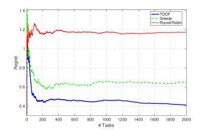
Fig. 2: Average regret versus time. The regret is calculated as $R(T):=\frac{1}{T}\sum_{t=1}^{T}r_{t}$.

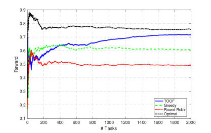
Fig. 3: Average reward versus time. The reward is calculated as $\tilde{R}(T):=\frac{1}{T}\sum_{t=1}^{T}\mathds{1}\{y_{I_{t}}^{(t)}=1\}$.

In Fig. 2, we compare the performance of the TOOF algorithm with Round-Robin and Greedy. In the round-robin algorithm, nodes are chosen in a cyclic sequence regardless of their current states. In the greedy algorithm, the task node chooses a helper node in each time slot under the same rule as TOOF, but $Z_{t}$ stays the same over time. It means that each single element of the estimated weight vector $\bar{\bm{w}}_{i}$ is updated in the same pace. Clearly, Fig. 2 indicates that our proposed TOOF algorithm shows the tendency of converging to zero. Besides, the TOOF algorithm achieves much lower regret than the other two algorithms.

The superior performance of our proposed scheme is also shown in Fig. 3. Comparing with (4), we find that the reward defined in Fig. 3 is also a happiness metric by denoting happy (unhappy) by $y_{I_{t}}^{(t)}=1(0)$. In Fig. 3, Optimal shows the performance in the case of perfect knowledge, where the node is chosen as (17). Note that the regret of Optimal is a zero value function. Our algorithm begins to show its superiority to the greedy algorithm since time slot-$400$ and keeps widening the gap. Fig. 3 also illustrates that the reward obtained via the TOOF algorithm approaches the optimal one. This shows that, with the increment of the number of tasks, our TOOF algorithm is capable of dealing with the tradeoff between learning system parameters and getting a high immediate reward.

6 Conclusions

In this paper, we have investigated an efficient task offloading strategy with one-bit feedback and have established the corresponding performance guarantee. Without knowing weight vectors of the helper nodes, with the probabilistic feedbacks, a multi-armed bandit framework has been formulated. Under the framework, we have proposed an efficient TOOF algorithm basing on the UCB policy. We have also proven that the upper bound of the average regret function is in the order of $O(\sqrt{(\log t)/t})$. Numerical simulations also demonstrate that our TOOF algorithm is able to obtain superior performance in an online fashion.

7 Appendix

The following inequality always holds due to that ${\bm{w}}_{I_{t}}$ and ${\bm{x}}_{I_{t}}^{(t)}$ have been normalized unitary:

$$\begin{split}r_{t}=&{\bm{w}}_{I_{t}^{*}}^{\top}{\bm{x}}_{I_{t}^{*}}^{(t)}-{\bm{w}}_{I_{t}}^{\top}{\bm{x}}_{I_{t}}^{(t)}\\ =&{\bm{w}}_{I_{t}^{*}}^{\top}({\bm{x}}_{I_{t}^{*}}^{(t)}-{\bm{x}}_{I_{t}}^{(t)})+({\bm{w}}_{I_{t}^{*}}-{\bm{w}}_{I_{t}})^{\top}{\bm{x}}_{I_{t}}^{(t)}\leq 4.\end{split}$$ (20)

On the other hand, with a probability at least $(1-\delta)$, the instantaneous regret $r_{t}$ can be upper-bounded as follows.

$$\begin{split}r_{t}&={\bm{w}}_{I_{t}^{*}}^{\top}{\bm{x}}_{I_{t}^{*}}^{(t)}-{\bm{w}}_{I_{t}}^{\top}{\bm{x}}_{I_{t}}^{(t)}\\ &\leq(\hat{\bm{w}}_{I_{t}}^{(t)}-\bar{\bm{w}}_{I_{t}}^{(t)})^{\top}{\bm{x}}_{I_{t}}^{(t)}+(\bar{\bm{w}}_{I_{t}}^{(t)}-{\bm{w}}_{I_{t}})^{\top}{\bm{x}}_{I_{t}}^{(t)}\\ &\overset{(a)}{\leq}\left(\|\hat{\bm{w}}_{I_{t}}^{(t)}-\bar{\bm{w}}_{I_{t}}^{(t)}\|_{\bm{Z}^{(t)}_{i}}+\|\bar{\bm{w}}_{I_{t}}^{(t)}-{\bm{w}}_{I_{t}}\|_{\bm{Z}^{(t)}_{i}}\right)\|{\bm{x}}_{I_{t}}^{(t)}\|_{(\bm{Z}^{(t)}_{i})^{-1}}\\ &\overset{(b)}{\leq}2\sqrt{\gamma_{i}^{(t)}}\|{\bm{x}}_{I_{t}}^{(t)}\|_{(\bm{Z}^{(t)}_{I_{t}})^{-1}}.\end{split}$$

where $(a)$ holds due to the Cauchy–Schwarz inequality, and $(b)$ holds with a probability at least $(1-\delta)$ referring to Proposition 1. Then the total regret can be upper-bounded by

$$\begin{split}&\sum_{t=1}^{T}r_{t}=\sum_{t=1}^{T}\left({\bm{w}}_{I_{t}^{*}}^{\top}{\bm{x}}_{I_{t}^{*}}^{(t)}-{\bm{w}}_{I_{t}}^{\top}{\bm{x}}_{I_{t}}^{(t)}\right)\\ &\leq\sum_{t=1}^{T}\min\left(2\sqrt{\gamma^{(t)}}\|\bm{x}_{I_{t}}^{(t)}\|_{(\bm{Z}_{I_{t}}^{(t)})^{-1}},4\right)\\ &\leq\sqrt{\frac{8\gamma^{(T)}}{\beta}}\max\left(1,\sqrt{2\beta}R\right)\sum_{t=1}^{T}\min\left(\sqrt{\frac{\beta}{2}}\|\bm{x}_{I_{t}}^{(t)}\|_{(\bm{Z}_{I_{t}}^{(t)})^{-1}},1\right)\\ &\leq\sqrt{\frac{8\gamma^{(T)}T}{\beta}}\sqrt{\sum_{t=1}^{T}\min\left({\frac{\beta}{2}}\|\bm{x}_{I_{t}}^{(t)}\|^{2}_{(\bm{Z}_{I_{t}}^{(t)})^{-1}},1\right)}.\\ \end{split}\vspace{-3mm}$$ (21)

Similar to the result from Lemma 11 in [16], we have

$$\begin{split}&\det\left(\bm{Z}_{i}^{(T+1)}\right)\\ &=\det\left(\bm{Z}_{i}^{(T)}+\frac{\beta}{2}\bm{x}_{i}^{(T)}(\bm{x}_{i}^{(T)})^{\top}\mathds{1}\{I_{T}=i\}\right)\\ &=\det\left(\bm{Z}_{i}^{(T)}\right)\left(1+\frac{\beta}{2}\|\bm{x}_{i}^{(T)}\|^{2}_{(\bm{Z}_{i}^{(T)})^{-1}}\mathds{1}\{I_{T}=i\}\right)\\ &=\det\left(\bm{Z}_{i}^{(1)}\right)\prod_{t=1}^{T}\left(1+\frac{\beta}{2}\|\bm{x}_{i}^{(t)}\|^{2}_{(\bm{Z}_{i}^{(t)})^{-1}}\mathds{1}\{I_{t}=i\}\right).\end{split}$$ (22)

Thus we have

$$\begin{split}&\sum_{t=1}^{T}\min\left({\frac{\beta}{2}}\|\bm{x}_{I_{t}}^{(t)}\|^{2}_{(\bm{Z}_{I_{t}}^{(t)})^{-1}},1\right)\\ &\leq 2\sum_{t=1}^{T}\log\left(1+{\frac{\beta}{2}}\|\bm{x}_{I_{t}}^{(t)}\|^{2}_{(\bm{Z}_{I_{t}}^{(t)})^{-1}}\right)\\ &=2\sum_{t=1}^{T}\sum_{i=1}^{K}\log\left(1+{\frac{\beta}{2}}\|\bm{x}_{i}^{(t)}\|^{2}_{(\bm{Z}_{i}^{(t)})^{-1}}\mathds{1}\{I_{t}=i\}\right)\\ &=2\sum_{i=1}^{K}\log\frac{\det\left(\bm{Z}_{i}^{(T)}\right)}{\det\left(\bm{Z}_{i}^{(1)}\right)}.\end{split}$$ (23)

Taking this result to (21) yields

$$\sum_{t=1}^{T}r_{t}\leq 4\sqrt{\frac{\gamma^{(T)}T}{\beta}\sum_{i=1}^{K}\log\frac{\det(\bm{Z}_{i}^{(T)})}{\det(\bm{Z}_{i}^{(1)})}}.\\$$ (24)

References

- [1] M. Chiang and T. Zhang, “Fog and IoT: An overview of research opportunities,” IEEE Internet Things J., vol. 3, no. 6, pp. 854–864, Dec. 2016.
- [2] T. Q. Dinh, J. Tang, Q. D. La, and T. Q. S. Quek, “Offloading in mobile edge computing: Task allocation and computational frequency scaling,” IEEE Trans. Commun., vol. 65, no. 8, pp. 3571–3584, Aug. 2017.
- [3] Y. Mao, C. You, J. Zhang, K. Huang, and K. B. Letaief, “A survey on mobile edge computing: The communication perspective,” IEEE Commun. Surveys Tuts., vol. 19, no. 4, pp. 2322–2358, Aug. 2017.
- [4] Y. Yang, K. Wang, G. Zhang, X. Chen, X. Luo, and M. Zhou, “MEETS: Maximal energy efficient task scheduling in homogeneous fog networks,” submitted to IEEE Internet Things J., 2017.
- [5] C. You, K. Huang, H. Chae, and B.-H. Kim, “Energy-efficient resource allocation for mobile-edge computation offloading,” IEEE Trans. Wireless Commun., vol. 16, no. 3, pp. 1397–1411, Mar. 2017.
- [6] J. Kwak, Y. Kim, J. Lee, and S. Chong, “DREAM: Dynamic resource and task allocation for energy minimization in mobile cloud systems,” IEEE J. Sel. Areas Commun., vol. 33, no. 12, pp. 2510–2523, Dec. 2015.
- [7] Y. Mao, J. Zhang, S. H. Song, and K. B. Letaief, “Stochastic joint radio and computational resource management for multi-user mobile-edge computing systems,” IEEE Trans. Wireless Commun., vol. 16, no. 9, pp. 5994–6009, Sept. 2017.
- [8] Y. Yang, S. Zhao, W. Zhang, Y. Chen, X. Luo, and J. Wang, “DEBTS: Delay energy balanced task scheduling in homogeneous fog networks,” IEEE Internet Things J., vol. 5, no. 3, pp. 2094-2016, Jun. 2018.
- [9] L. Pu, X. Chen, J. Xu, and X. Fu, “D2D fogging: An energy-efficient and incentive-aware task offloading framework via network-assisted D2D collaboration,” IEEE J. Sel. Areas Commun., vol. 34, no.12, pp. 3887–3901, Dec. 2016.
- [10] T. Chen and G. B. Giannakis, “Bandit convex optimization for scalable and dynamic IoT management”, IEEE Internet Things J., in press.
- [11] Z. Zhu, T. Liu, S. Jin, and X. Luo, “Learn and pick right nodes to offload”, arXiv preprint arXiv:1804.08416, 2018.
- [12] P. Auer, N. Cesa-Bianchi, and P. Fischer, “Finite-time analysis of the multiarmed bandit problem,” Mach. Learn., vol. 47, no. 2, pp. 235–256, May 2002.
- [13] D. A. Berry and B. Fristedt, Bandit Problems: Sequential Allocation of Experiments. London, U.K.: Chapman & Hall, 1985.
- [14] S. Bubeck and N. Cesa-Bianchi, “Regret analysis of stochastic and nonstochastic multi-armed bandit problems,” Found. Trends Mach. Learn., vol. 5, no. 1, pp. 1–122, 2012.
- [15] L. Zhang, T. Yang, R. Jin, Y. Xiao, and Z. Zhou, “Online stochastic linear optimization under one-bit feedback,” Proc. ICML, New York, NY, USA, Jun. 2016, pp. 392–401.
- [16] Y. Abbasi-Yadkori, D. Pál, and C. Szepesvári, “Improved algorithms for linear stochastic bandits,” Advances in Neural Information Processing Systems, Granada, Spain, Dec. 2011.