Notes on ten-dimensional localized black holes and deconfined states in two-dimensional SYM

Abstract

We numerically construct static localized black holes in ten spacetime dimensions with one compact periodic dimension. In particular, we investigate the critical regime in which the poles of the localized black hole are about to merge. When approaching the critical region, the behavior of physical quantities is described by a single real valued exponent giving rise to a logarithmic scaling of the thermodynamic quantities, in agreement with the theoretical prediction derived from the double-cone metric. As a peculiarity, the localized black hole solution in ten dimensions can be related to the spatially deconfined phase of two dimensional $\mathcal{N}=\left(8,8\right)$ super Yang-Mills theory (SYM) on a spatial circle. We use the localized black hole solutions to determine the SYM phase diagram. In particular, we compute the location of the first order phase confinement/deconfinement transition and the related latent heat to unprecedented accuracy.

1 Introduction and Summary

Throughout the last decades, the topic of black holes in higher dimensional spacetime with $D>4$ attracted a lot of attention. Special focus was devoted to the study of $D$-dimensional black objects in spacetimes with one periodic dimension, called Kaluza-Klein black holes. In this context there are various solutions to Einstein’s vacuum equations with different horizon topologies, such as black strings and localized black holes. The former are extended along the entire compact dimension while the latter are localized there.

Uniform black strings are unstable below a certain mass [1, 2]. From this instability the branch of non-uniform black strings arises, which a number of authors have constructed in different dimensions using perturbative and numerical techniques [3, 4, 5, 6, 7, 8, 9, 10, 11, 12]. However, thermodynamic arguments show that localized black holes are a more stable configuration for small masses. Such solutions have been constructed perturbatively and numerically only in $D=5,\,6$ [13, 14, 15, 16, 17, 18, 19, 20, 8, 21] and recently in $D=10$ [12]. Altogether this leads to an interesting and rather involved phase diagram of static Kaluza-Klein black holes. Good reviews summarizing the scientific progress in this realm can be found in references [22, 23, 24, 25].

In particular, recent work shed new light on this topic, showing that the solution branches of non-uniform black strings and localized black holes converge towards each other and that this transition is controlled by complex critical exponents [10, 11, 21]. Interestingly, this critical behavior can be deduced from the so-called double-cone metric, which Kol proposed as a local model of the transit solution between non-uniform black strings and localized black holes [26, 27].

While these recent results only concern the dimensions $D=5,\,6$, the present work concentrates on the construction of localized black holes in $D=10$ based on the methods presented in [21]. Special attention is devoted to the critical regime, where the poles of the horizons are about to merge along the compact dimension. In particular, we show that the critical regime in $D=10$ is approached in a qualitatively different manner than for $D=5,\,6$, i.e. without oscillations. Moreover, the obtained value of the real critical exponent is in excellent agreement with the value that was predicted by Kol [26, 27].

In a second strand of the paper we investigate the phase diagram of maximally supersymmetric, two-dimensional super Yang-Mills theory (SYM) on a spatial circle $\mathbb{S}^{1}$ at strong coupling by the virtue of the AdS/CFT correspondence [28, 29]. Due to the relation of the $D=10$ dimensional black hole and black string solutions to thermal states of the SYM [30, 31, 12], we are able to determine the phase diagram of the dual quantum field theory. While black strings correspond to spatially confined phases, the localized black hole solution is dual to a deconfined phase. We locate the first order phase transition between deconfined and confined phases in the microcanonical and canonical ensemble with extraordinary accuracy. In addition, we calculate the latent the heat of the phase transition and find a critical behavior where the two meta-stable branches merge. All together, these quantities provide valuable predictions for calculations within lattice quantum field theory (see e.g. [32, 33, 34]).

The paper is structured as follows: We review the physical setup for localized black holes in ten-dimensional asymptotically flat spacetimes in section 2. As in reference [21], the heart of our numerical implementation is a multi-domain pseudo-spectral method. In section 2.2 we present our main results and compare the extracted critical exponent with the theoretical predictions. As a second strand of the paper we study two-dimensional maximally supersymmetric Yang-Mills theory using the conjectured gauge/gravity duality in section 3. In particular, we determine its phase diagram in 3.1, and investigate the critical regime in the dual SYM in section 3.2.

We provide supplementary material in appendix A concerning the numerical implementation and the calculation of the phase transition points. Moreover, in appendix B we review the supergravity description of the two-dimensional maximally supersymmetric Yang-Mills theory and its regime of validity.

Note added: While this paper was being completed we became aware of upcoming work discussing similar issues [35].

2 Localized black holes in ten dimensions

This section is devoted to localized black hole solutions arising from pure general relativity in ten dimensions with one compact spatial dimension. The ansatz for their numerical construction is outlined in subsection 2.1, while we postpone a more detailed description of the numerics to appendix A. We utilized the numerical scheme developed in reference [21] and only made some minor adaptions. We present the results of our computations in the localized black hole context in subsection 2.2.

2.1 Ansatz for the metric

We consider ten-dimensional solutions of Einstein’s vacuum field equations $R_{\mu\nu}=0$, where one of the spatial dimensions is curled up to a circle of size $L$. The simplest solution reads

$$\mathrm{d}s^{2}=-\mathrm{d}t^{2}+\mathrm{d}x^{2}+x^{2}\,\mathrm{d}\Omega^{2}_{7}+\mathrm{d}y^{2}\,.$$ (1)

Obviously, there is a spherical symmetry on the spatially extended dimensions with the radial coordinate $x\in[0,\infty]$. The additional coordinate $y$ is compact, $y\in[0,L]$, and periodically identified, i.e. $y\simeq y+L$. This metric is a direct product of nine-dimensional Minkowski spacetime and a circle $\mathbb{S}^{1}$. Therefore, it serves as the background metric, which all other solutions shall approach in the asymptotic limit $x\to\infty$.

Keeping the spherical symmetry and, moreover, restricting ourselves to static solutions, a general metric ansatz which incorporates the required symmetries reads

$$\mathrm{d}s^{2}=-T_{\mathrm{a}}\,\mathrm{d}t^{2}+A_{\mathrm{a}}\,\mathrm{d}x^{2}+B_{\mathrm{a}}\,\mathrm{d}y^{2}+2\,F_{\mathrm{a}}\,\mathrm{d}x\,\mathrm{d}y+x^{2}S_{\mathrm{a}}\,\mathrm{d}\Omega^{2}_{7}\,.$$ (2)

The five metric functions $T_{\mathrm{a}}$, $A_{\mathrm{a}}$, $B_{\mathrm{a}}$, $F_{\mathrm{a}}$ and $S_{\mathrm{a}}$ depend on $x$ and $y$. We obtain two asymptotic charges, the mass $M$ and the relative tension $n$, from the subleading behavior of the metric (2) at infinity. In fact, these two quantities are related to the coefficients $c_{t}$ and $c_{y}$ defined by

$$T_{\mathrm{a}}\simeq 1-c_{t}\,\frac{L^{6}}{x^{6}}\,,\quad{}B_{\mathrm{a}}\simeq 1+c_{y}\,\frac{L^{6}}{x^{6}}\,,$$ (3)

in the following way

$$M=\frac{L^{7}\,\Omega_{7}}{16\pi G_{10}}\,\left(7c_{t}-c_{y}\right)\,,\quad n=\frac{c_{t}-7\,c_{y}}{7\,c_{t}-c_{y}}\,.$$ (4)

Note that the relative tension describes the force by which an object tries to compress the compact dimension.

There are at least two types of static black hole solutions in Kaluza-Klein theory: black strings, which are extended all over the compact dimension and localized black holes, which are smaller than the compact dimension. For the latter ones, being the subject of this work, the coordinates used in the metric (2) are not appropriate to describe their near horizon behavior, since the horizon is some curved contour in the $(x,y)$-plane. For this reason, we introduce polar coordinates $(\varrho,\varphi)$ via $x=\varrho\sin\varphi$ and $y=\varrho\cos\varphi$, and rewrite the metric as

$$\mathrm{d}s^{2}=-\kappa^{2}(\varrho-\varrho_{0})^{2}T_{\mathrm{h}}\,\mathrm{d}t^{2}+A_{\mathrm{h}}\,\mathrm{d}\varrho^{2}+\varrho^{2}B_{\mathrm{h}}\,\mathrm{d}\varphi^{2}+2\,\varrho F_{\mathrm{h}}\,\mathrm{d}\varrho\,\mathrm{d}\varphi+\varrho^{2}\sin^{2}\varphi S_{\mathrm{h}}\,\mathrm{d}\Omega^{2}_{7}\,.$$ (5)

The functions $T_{\mathrm{h}}$, $A_{\mathrm{h}}$, $B_{\mathrm{h}}$, $F_{\mathrm{h}}$ and $S_{\mathrm{h}}$ depend on $\varrho$ and $\varphi$, and are connected with their counterparts of the metric (2) in a linear way. By the extraction of the term $\kappa^{2}(\varrho-\varrho_{0})^{2}$ from the $tt$-component of the metric we ensure that the horizon is located at $x^{2}+y^{2}=\varrho^{2}=\varrho_{0}^{2}$. In fact, this is only a gauge choice in a sense that we want the horizon to have a spherical shape in the $(x,y)$ chart but the ’true’ horizon shape will not necessarily be exactly spherical. Thus, the parameter $\varrho_{0}$ does not have a specific physical meaning. In contrast, the surface gravity $\kappa$ determines physically inequivalent solutions.

Our numerical approach to find localized black hole solutions relies both on the metric (2) and the metric (5), which we call the asymptotic and the near horizon chart, respectively. This has the advantage of having coordinates and metric functions that are well suited to different regions of the spacetime. We postpone an outline of the numerical scheme to appendix A.

Besides the asymptotic charges there are some more physical quantities of interest, in particular the temperature $T$ and the entropy $S$ of the black hole. While the temperature is simply related to the surface gravity via $T=\kappa/(2\pi)$, the entropy is proportional to the surface area of the horizon. In what follows we consider the following dimensionless normalization of the physical quantities:

$$\tilde{M}=\frac{G_{10}\,M}{L^{7}}\,,\qquad\tilde{T}=TL\,,\qquad\tilde{S}=\frac{G_{10}\,S}{L^{8}}\,.$$ (6)

2.2 Thermodynamics and critical behavior

We show the phase diagram of localized black holes in ten dimensions in figure 1 for the microcanonical and canonical ensemble. The comparison with uniform black strings reveals that localized black holes are thermodynamically favored for small masses and large temperatures. Note that reference [12] did already show this picture qualitatively and, moreover, included the non-uniform black string results into the diagram. However, we were able to extend the localized black hole solutions much closer to the end point of this branch, where a transition to non-uniform black strings is expected. Moreover, we are able to extract the position of the first order phase transition (the point where the uniform black string branch and the localized black hole branch cross each other) from our data with high accuracy by distributing the data points around this intersection on a Lobatto grid, see appendix section A.4 for more details. In the microcanonical ensemble we obtain

$$\tilde{M}_{\text{PT}}=0.01369926356406(1)\,,$$ (7)

whereas in the canonical ensemble we get

$$\tilde{T}_{\text{PT}}=1.267669090870(1)\,.$$ (8)

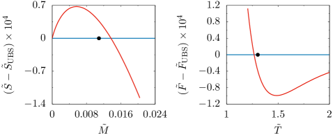
Figure 1: Phase diagram of 10-dimensional localized black holes in the microcanonical (left) and canonical (right) ensemble. We plot the difference of entropy and free energy, respectively, to the corresponding values of the uniform black string, which is thus represented as the blue zero line in these diagrams with the black circle indicating the solution where the Gregory-Laflamme instability arises. The branch of localized black holes, represented by the red line, is thermodynamically favored over the uniform black strings for small masses or high temperatures.

We now turn our attention to the end point of the localized black hole branch. Following this branch it turns out that the black hole horizon spreads more and more along the compact dimension. The transition to non-uniform black strings is believed to be controlled by the so-called double-cone metric [26], which is a local model of the spacetime at the point where the poles of the localized black hole touch each other. Indeed, figure 2 shows how the localized black hole horizon approaches the double-cone locally. These horizon shapes were obtained by embedding the horizons of different localized black hole solutions into flat space, cf. references [21, 25] for more details.

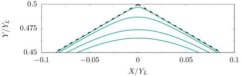
Figure 2: Local convergence towards the double-cone horizon shape. We embed the horizons of different localized black holes solutions into nine-dimensional flat space and display two-dimensional cross-sections disregarding the seven-dimensional spherical symmetry. The non-trivial directions $X$ and $Y$ correspond to our spacetime coordinates $x$ and $y$. In the region close to the edge of the compact dimension, $Y\lesssim Y_{L}/2$, we see that the shape predicted by the double-cone metric (dashed line) is nicely approached by localized black hole horizons (green lines) for increasing mass or decreasing temperature, respectively.

Another interesting conjecture in the context of the double-cone metric is the occurrence of critical exponents that control the thermodynamics when the black hole/black string transition is approached [26, 27]. More concretely, we expect a certain physical quantity $p$ in this regime to scale as

$$f-f_{\text{c}}=A\,Q^{-s_{+}}+B\,Q^{-s_{-}}\,,\quad{}\text{with}\quad{}s_{\pm}=-\frac{D-2}{2}\left(-1\pm\text{i}\sqrt{\frac{8}{D-2}-1}\right)\,,$$ (9)

where $Q$ is a typical length scale controlling the transition, $a$ and $b$ are constants and $f_{\text{c}}$ is the value of the quantity $f$ at the transition. While for dimensions $D<10$ the exponents $s_{\pm}$ are complex and hence lead to damped oscillations of physical quantities, they become purely real for $D\geq 10$. For $D=5,6$ this expectation was explicitly confirmed in reference [21]. In the case considered here, $D=10$, the exponents $s_{\pm}$ degenerate, $s_{-}=s_{+}$, and hence the scaling law (9) has to be modified as follows

$$f(Q)=f_{\text{c}}-Q^{b}(a_{1}+a_{2}\,\log Q)\,,$$ (10)

with $b=4$. Moreover, $a_{1}$ and $a_{2}$ are constants.

Table 1: Fit parameters for the function $f(Q)=f_{\text{c}}-Q^{b}\,(a_{1}+a_{2}\,\log Q)$ where $f$ stands for different physical quantities and $Q=L_{\mathcal{A}}/L$. The fit parameters were determined using all data points with $Q\lesssim 0.02$.

$f$	$f_{c}$	$b$	$a_{1}$	$a_{2}$
$\tilde{M}$	0.020404622	4.0009	0.2125	-1.1380
$n$	0.019873805	3.9999	-7.8223	-6.1737
$\tilde{T}$	1.205852954	4.0006	-0.5245	10.8728
$\tilde{S}$	0.014764118	4.0009	0.1757	-0.9440

In order to check this conjecture we follow reference [21] and fit our data for the ten-dimensional localized black holes with the ansatz (10) leaving $f_{\text{c}}$, $b$, $a_{1}$ and $a_{2}$ as free parameters to be determined by the fit routine. We use the proper distance between the poles $L_{\mathcal{A}}$ as the length scale to describe the transition, as $L_{\mathcal{A}}=0$ when the transition is reached. Accordingly, we set $Q=L_{\mathcal{A}}/L$. Table 1 shows the obtained fit parameter values for different physical quantities. Most importantly, the theoretical predicted value $b=4$ is confirmed to great accuracy. Moreover, we display the good agreement of data points and fit exemplarily for the mass in figure 3.

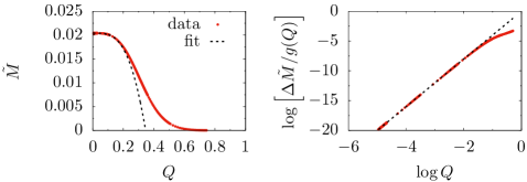
Figure 3: Scaling of mass. We show the rescaled mass $\tilde{M}$ as a function of the normalized proper distance between the poles $Q=L_{\mathcal{A}}/L$ (left). To illustrate the remarkable agreement of data points and fit, we plot the mass difference $\Delta\tilde{M}=\tilde{M}_{0}-\tilde{M}$ divided by $g(Q)=a_{1}+a_{2}\,\log Q$ against $Q$ in a double logarithmic diagram (right).

3 Thermal states of $\mathcal{N}=(8,8)$ SYM and localized black holes

Via the renowned gauge/gravity duality conjecture, Kaluza-Klein black holes in $D=10$ are related to thermal states of a two-dimensional $\mathcal{N}=\left(8,8\right)$ supersymmetric Yang-Mills (SYM) theory compactified to a circle $\mathbb{S}^{1}$ with gauge group $SU(N)$ in the large $N$ limit. In particular, localized black holes correspond to a spatially deconfined phase within the SYM, while black strings are related to spatially confined phases.

Note that the aforementioned SYM can be characterized by three dimensionless quantities: The rank of the gauge group $N$, the dimensionless ’t Hooft coupling constant $\lambda=Ng_{YM}^{2}L^{2}$ and the dimensionless temperature $\mathcal{T}$ given by the product of the ordinary temperature and the length of the circle $L$. In the following, we denote the (dimensionless) thermodynamic quantities of the SYM by $\mathcal{U}$ for the energy, $\mathcal{T}$ for the temperature and $\mathcal{S}$ for the entropy.

According to [30, 31, 12], the localized black holes and black strings in $D=10$ dimensional asymptotically flat spacetime with one compact periodic dimension discussed in section 2 can be related to the gravitational dual solution of SYM states by employing the the following solution generating technique:

1. First, we lift the $D=10$ dimensional solutions of vacuum Einstein equations discussed in section 2 to $D=11$ dimensions and perform a boost in the new coordinate, followed by a subsequent Kaluza-Klein reduction.

   The result is a solution in type IIA supergravity. Concretely, the localized black hole solutions in $D=10$ with $\mathbb{R}^{1,8}\times\mathbb{S}^{1}$ asymptotics correspond to localized D0-branes in type IIA supergravity.

2. As a next step a T-duality transformation is applied, which converts the type IIA supergravity solution into a type IIB supergravity solution.

3. As a last step we take the decoupling limit between the string and gravitational length scales on the type IIB gravity side, which corresponds to taking the limit $N\rightarrow\infty$ with $\lambda$ fixed on the SYM side, and to consider the large $\lambda$ limit in a second step.

The details of the decoupling limit are rather complicated and we refer the reader to the references [30, 31, 12] and appendix  B for a thorough description of the underlying limits and an analysis on the validity of the supergravity description of the SYM states.

We determine the phase diagram of the $\mathcal{N}=\left(8,8\right)$ SYM compactified to a circle $\mathbb{S}^{1}$ in section 3.1 by applying the solution generating to the ten-dimensional localized black holes in asymptotically flat spacetime. In particular we locate the first order phase transition to very high accuracy. Moreover, in 3.2 we interpret the critical regime between localized black holes and non-uniform black strings as an emergent critical scaling behavior related to the first order phase transition where the the two meta-stable branches merge.

3.1 Thermodynamic quantities

As a result of the solution generating procedure, we can relate the thermodynamic quantities of the SYM to the thermodynamic properties of the Kaluza-Klein black holes. In particular, considering the normalized quantities $\mathcal{\tilde{U}}=\mathcal{U}\cdot\lambda^{2}/N^{2}$, $\mathcal{\tilde{T}}=\mathcal{T}\cdot\lambda^{1/2}$ and $\mathcal{\tilde{S}}=\mathcal{S}\cdot\lambda^{3/2}/N^{2}$, we obtain (cf. reference [12])

$$\mathcal{\tilde{U}}=64\,\pi^{4}\left(2\tilde{M}-\tilde{S}\tilde{T}\right)\,,\qquad\mathcal{\tilde{T}}=4\sqrt{2}\pi\tilde{S}^{1/2}\tilde{T}^{3/2}\,,\qquad\mathcal{\tilde{S}}=16\sqrt{2}\pi^{3}\sqrt{\frac{\tilde{S}}{\tilde{T}}}\,.$$ (11)

The free energy $\mathcal{F}$ of the canonical ensemble and its normalized version $\mathcal{\tilde{F}}=\mathcal{F}\cdot\lambda^{2}/N^{2}$ are given by $\mathcal{F}=\mathcal{U}-\mathcal{S}\mathcal{T}$ and $\mathcal{\tilde{F}}=\mathcal{\tilde{U}}-\mathcal{\tilde{S}}\mathcal{\tilde{T}}$.

Figure 4 shows the phase diagrams of the microcanonical and canonical ensembles of the uniform and localized phases of the $\mathcal{N}=\left(8,8\right)$ SYM. For the microcanonical ensemble, we see that the localized phase is thermodynamically preferred over the uniform phase up to some threshold value of the normalized internal energy $\tilde{\mathcal{U}}_{PT}$, where the uniform phase starts to dominate. There is a first order phase transition, where the entropy of the uniform phase exceeds the entropy of the localized branch. We have a similar picture when considering the canonical phase diagram. Here, lower values of the free energy $\mathcal{\tilde{\mathcal{F}}}$ correspond to the thermodynamically preferred phase. Accordingly, we see that the localized phase is dominating for small values of the normalized temperature $\tilde{\mathcal{T}}$. As before, the uniform phase becomes thermodynamically preferred at some threshold value $\tilde{\mathcal{T}}_{PT}$. We remark that including the SYM phases corresponding to non-uniform black strings will not alter this picture of thermodynamic stability, since the related branch is thermodynamically inferior for all configurations, as can be seen from the data presented in reference [12].

With the procedure described in appendix section A.4 we determine the first order phase transition between the localized and the uniform phase in the microcanonical ensemble to be at

$$\mathcal{\tilde{U}}_{\text{PT}}=96.9053906163(1)\,.$$ (12)

For the canonical ensemble we find

$$\mathcal{\tilde{T}}_{\text{PT}}=2.451118333749(1)\,.$$ (13)

Both values are in good agreement with reference [12] which determines $\mathcal{\tilde{U}}_{\text{PT}}\approx 97.067$ and $\mathcal{\tilde{T}}_{\text{PT}}\approx 2.451$. Moreover, the latent heat associated with the first order phase transition between localized black holes and uniform black strings (UBS) is given by

$$\Delta\mathcal{\tilde{Q}} =\mathcal{\tilde{T}}_{\text{PT}}\,\cdot\,\left(\mathcal{\tilde{S}}_{\mathrm{UBS}}-\mathcal{\tilde{S}}\right)\Big{|}_{\mathcal{\tilde{T}}=\mathcal{\tilde{T}}_{\text{PT}}}$$ (14a)

$$=\mathcal{\tilde{T}}_{\text{PT}}\,\cdot\,\frac{\partial(\mathcal{\tilde{F}}-\mathcal{\tilde{F}}_{\mathrm{UBS}})}{\partial\mathcal{\tilde{T}}}\Big{|}_{\mathcal{\tilde{T}}=\mathcal{\tilde{T}}_{\text{PT}}}$$ (14b)

where $\mathcal{\tilde{S}}(\mathcal{\tilde{T}})$ is the normalized entropy associated with the localized black holes. Utilizing again the procedure described in appendix section A.4 we determine the latent heat to be

$$\Delta\mathcal{\tilde{Q}}=9.47738683316(1)\,.$$ (15)

Note that this value was obtained from equation (14a). We also evaluated equation (14b) and only found deviations within the last two digits compared to the value given in equation (15), which is completely expected since in this case we have to perform a numerical derivative of the free energy.

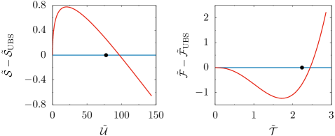
Figure 4: Phase diagram of $\mathcal{N}=(8,8)$ SYM on a circle with length $L$ in the microcanonical (left) and canonical (right) ensemble. We plot the difference of entropy and free energy, respectively, to the corresponding values of the uniform branch, which is thus represented as the blue zero line in these diagrams with the black circle indicating the solution where the Gregory-Laflamme instability arises. The localized branch, represented by the red line, is thermodynamically favored over the uniform branch for small masses or small temperatures.

Again, when approaching the end point of the localized branch, the physical quantities show a scaling behavior, reminiscent of the one for the localized black holes in ten dimensional Kaluza-Klein geometries. While this is expected from the gravitational point of view, cf. reference [27], this is surprising from the field theory perspective. To our best knowledge, we are not aware of results in the literature concerning an emergent scaling behaviour with real critical exponents when the two meta-stable branches merge into each other.

In table 2 we list these unexpected critical exponents (see third column) which were obtained by fitting our data with the same ansatz (10) as we used for the localized black holes.

Table 2: Fit parameters for the function $f(Q)=f_{\text{c}}-Q^{b}\,(a_{1}+a_{2}\,\log Q)$ where $f$ stands for different physical quantities and $Q=L_{\mathcal{A}}/L$. The fit parameters were determined using all data points with $Q\lesssim 0.02$.

$f$	$f_{c}$	$b$	$a_{1}$	$a_{2}$
$\mathcal{\tilde{U}}$	143.42290	4.0009	1362	-8100
$\mathcal{\tilde{T}}$	2.8593686	4.0008	15.46	-52.60
$\mathcal{\tilde{S}}$	77.632071	4.0008	480.1	-2831
$\mathcal{\tilde{F}}$	-78.555803	4.0010	-1188	4088

3.2 Lessons for the dual SYM

We obtained the phase diagrams of the localized and uniform phases of the two-dimensional $\mathcal{N}=\left(8,8\right)$ supersymmetric SYM theory compactified to a circle $\mathbb{S}^{1}$ with gauge group $SU(N)$ in the large $N$ limit from the corresponding localized black hole and uniform black string solutions. The localized branch was found to be predominating for small energies or temperatures, whereas the uniform phase becomes thermodynamically favored at some threshold values of the energy $\tilde{\mathcal{U}}_{PT}$ or temperature $\tilde{\mathcal{T}}_{PT}$. We obtained the threshold values with unprecedented accuracy and additionally computed the latent heat $\Delta\tilde{\mathcal{Q}}$ of the related first order phase transition.

Especially the values $\tilde{\mathcal{U}}_{PT}$, $\tilde{\mathcal{T}}_{PT}$ and $\Delta\tilde{\mathcal{Q}}$ are the basis for a comparison of our results with regarding data from quantum lattice calculations. We refer the reader to the references [32, 33, 34] for lattice results that show indications of a first-order phase transition. We remark, that possible phase transitions within this theory, are detected within lattice calculations by considering the Polyakov loop $P_{L}$ for a closed curve $\mathcal{C}_{L}$ along the periodic spatial direction

$$P_{L} =\frac{1}{N}\left\langle\textrm{Tr}\,\mathcal{P}\exp\left(\text{i}\oint_{\mathcal{C}_{L}}A\right)\right\rangle\,,$$ (16)

where $\mathcal{P}$ indicates the usual ordering prescription for Polyakov and Wilson loops. $P_{L}$ is an order parameter for a spatial confinement/deconfinement phase transition: $P_{L}\neq 0$ indicates a deconfined spatial behavior, while $P_{L}=0$ signals a confined spatial behavior. Within the dual supergravity theory, the localized black hole phase corresponds to a spatially deconfined phase with non-zero Polyakov loop $P_{L}\neq 0$ while the black string solutions are related to a spatially confined phases with $P_{L}=0$.

A more refined observable is the eigenvalue distribution of the Polyakov loop $P_{L}$ [30] on the complex unit circle. Note that the eigenvalue distribution is continuous in the large $N$ limit. This observable allows us to distinguish between states dual to localized black holes as well as non-uniform and uniform black strings. While uniform black strings are dual to a state with a homogeneous eigenvalue distribution on the complex unit circle, the non-uniform black strings correspond to a non-uniform eigenvalue distribution which is spread over the entire unit circle, i.e. for black strings we have the eigenvalues $\exp(\text{i}\varphi)$ for all $\varphi\in[-\pi,\pi]$.

In contrast, for the state dual to the localized black hole, we only have eigenvalues for $\varphi\in[-\varphi_{0},\varphi_{0}],$ where $\varphi_{0}<\pi$. In other words, the eigenvalue distribution is only nonzero for $|\varphi|\leq\varphi_{0}$. Hence, the state corresponding to the limiting case $\varphi_{0}\rightarrow\pi$ is dual to the merger solution in the gravitational theory, approached from the branch of the localized black holes. We expect that the scaling law (10), with $Q\sim\pi-\varphi_{0}$ and the critical exponents as reported in table 2, should emerge while interpolating between the localized and non-homogeneous eigenvalue distributions.

Appendix A Numerical details and convergence

Reference [21] gives a comprehensive discussion of how to construct localized black hole solutions in five and six spacetime dimensions very accurately. The setup that we utilized for the ten-dimensional case heavily relies on this approach. In subsection A.1 we only want to emphasize the corner stones of our numerical implementation while referring to reference [21] for more details. However, to extract the asymptotic charges accurately, we had to introduce some new techniques, which we explain in subsection A.2. In subsection A.3 we discuss the accuracy and the convergence of the numerical solutions. Finally, subsection A.4 shows how we obtained the highly accurate values regarding the phase transition from our data.

A.1 Overall scheme

We utilize the DeTurck method [8] in order to find numerical solutions to Einstein’s vacuum equations in the given context, see references [37, 38] for reviews. Hence, rather than solving these equations directly, we want to find solutions to the Einstein-DeTurck equations

$$R_{\mu\nu}-\nabla_{(\mu}\xi_{\nu)}=0\,,$$ (17)

with the DeTurck vector field $\xi$ defined by

$$\xi^{\mu}=g^{\alpha\beta}\left(\Gamma_{\alpha\beta}^{\mu}-\bar{\Gamma}_{\alpha\beta}^{\mu}\right)\,.$$ (18)

While $\Gamma$ is the usual Christoffel connection obtained from the desired spacetime metric $g$, $\bar{\Gamma}$ is the Christoffel connection associated with an unphysical reference metric $\bar{g}$ that only needs to exhibit the same causal structure and boundary conditions as $g$. If this is the case, a solution $g$ of the Einstein-DeTurck equations also satisfies Einstein’s vacuum equations, at least in the static case considered here [39]. Nevertheless, for a numerical solution $g$ it is always a good idea to check if the DeTurck vector is sufficiently close to zero, which ensures that the additional term in the Einstein-DeTurck equations vanishes.

To construct an appropriate reference metric we follow the lines of reference [21]: Observing that the background metric (1) already satisfies the right boundary conditions on all boundaries except the horizon, we simply take this metric as reference but only for $x^{2}+y^{2}=\varrho^{2}\geq\varrho_{1}^{2}$, see also reference [8]. Within $\varrho_{0}\leq\varrho\leq\varrho_{1}$ we construct the reference by matching it with the background metric at $\varrho=\varrho_{1}$ and with a ten-dimensional Schwarzschild-Tangherlini metric at $\varrho=\varrho_{0}$, see reference [21] for more details.

Our numerical approach relies on a pseudo-spectral method. In particular, we approximate all functions with a truncated series of Chebyshev polynomials of the first kind, while we demand that this approximation is exact on Lobatto grid points. With this we are able to utilize the Newton-Raphson method in order to solve the differential equations on the grid. The rate of convergence of a Chebyshev series heavily relies on smoothness properties of the underlying function. For this reason we decompose the domain of integration into several subdomains and perform appropriate coordinate transformations. The resulting grid setup is discussed in figure 5 but we refer to reference [21] for more details.

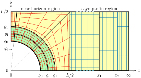
Figure 5: Grid structure for the construction of localized black hole solutions. For $x\leq L/2$ the computations are carried out with respect to the near horizon chart (5) (indicated by red grid lines) while for $x\geq L/2$ the asymptotic chart (2) is used (indicated by blue grid lines). For $\varrho\leq\varrho_{1}$ (green shaded region) we define a $\varphi$-independent reference metric that only contains powers of $\varrho$ by matching with the the ten-dimensional Schwarzschild-Tangherlini metric at the horizon $\varrho=\varrho_{0}$ and with the Kaluza-Klein background metric at $\varrho=\varrho_{1}$. Consequently, for $\varrho>\varrho_{1}$ (yellow shaded region) we simply use the Kaluza-Klein background as a reference. We introduce additional inner boundaries along $\varrho=\varrho_{\text{i}}$, $\varphi=\varphi_{\text{i}}$, $x=x_{1}$ and $x=x_{2}$ in order to be able to increase the numerical resolution especially near the horizon $\varrho=\varrho_{0}$, the exposed axis $\varphi=0$ and infinity $x\to\infty$. For the majority of our calculations we used the following parameter values: $L=8$, $\varrho_{0}=2$, $\varrho_{\text{i}}=2.5$, $\varrho_{1}=3$, $\varphi=0.1$, $x_{1}=L$ and $x_{2}=5\,L$. The reference metric itself can be used to construct an initial guess for the Newton-Raphson scheme with the above parameter values and $\kappa=1.4$. Once a first solution is found, different solutions are obtained by slightly perturbing $\kappa$ and using the old solution as an initial guess.

The domain of integration consists of five outer boundaries: the asymptotic boundary ($x\to\infty$), start and mid point of the compact dimension ($y=0$ and $y=L/2$), the symmetry axis ($x=0$) and the horizon ($x^{2}+y^{2}=\varrho_{0}^{2}$). We divide the domain of integration into an asymptotic region ($x\geq L/2$) and a near horizon region ($x\leq L/2$). In the former we consider the metric functions of the asymptotic chart (2), while in the latter it is more convenient to work with the polar coordinates in the near horizon chart (5).

The numerical method requires boundary conditions for all functions in each subdomain. On inner boundaries we simply demand equality of the metric function values and their normal derivatives with respect to neighboring subdomains. Conditions on the five outer boundaries mentioned above are obtained from regularity and symmetry requirements of the metric and are derived from the field equations itself, see reference [21] for the explicit conditions or reference [38] for a more general discussion of boundary conditions in the context of the DeTurck method. However, an exception is the asymptotic boundary, where the metric shall approach the background and therefore Dirichlet conditions are usually employed. As mentioned before, since we want to extract the asymptotic charges quite accurately, we use a more sophisticated approach here, which we explain in the next subsection.

A.2 Extraction of asymptotic charges

To obtain the asymptotic charges, mass and tension, we need to extract the coefficients $c_{t}$ and $c_{y}$ from the functions $T_{\mathrm{a}}$ and $B_{\mathrm{a}}$, cf. equation (3). Of course, we cover the integration domain up to infinity with an appropriate coordinate transformation that compactifies the asymptotic boundary to a finite coordinate value. This coordinate transformation reads $x(s)=L/(1-s)$ where $s\in[-1,1]$ covers the whole asymptotic region $x\in[L/2,\infty]$. Consequently, in principle it is possible to get the asymptotic coefficients $c_{t}$ and $c_{y}$ from the sixth derivative of the functions $T_{\mathrm{a}}$ and $B_{\mathrm{a}}$ with respect to $s$. However, since each numerical derivative is accompanied with some small errors, we cannot expect the sixth derivative to be reasonable accurate.

This is in contrast to the five- or six-dimensional approach, where only the first or second derivatives are involved and an accurate determination of the asymptotic coefficients is possible, see reference [21].

Therefore, in the ten-dimensional case we employ the following approach: We write the functions in the asymptotic chart $X_{\mathrm{a}}=\{T_{\mathrm{a}},A_{\mathrm{a}},B_{\mathrm{a}},S_{\mathrm{a}}\}$ and $F_{\mathrm{a}}$ as

$$X_{\mathrm{a}}=1+\frac{(1-s)^{5}}{32}\tilde{X_{\mathrm{a}}}\quad\text{and}\quad F_{\mathrm{a}}=\frac{(1-s)^{5}}{32}\tilde{F_{\mathrm{a}}}\,,$$ (19)

and now solve for the new functions $\tilde{X_{\mathrm{a}}}$ and $\tilde{F_{\mathrm{a}}}$. In this way we obtain the asymptotic coefficients $c_{t}$ and $c_{y}$ only from the first derivatives of the functions $\tilde{T_{\mathrm{a}}}$ and $\tilde{B_{\mathrm{a}}}$ at $s=1$. Note that the ansatz (19) incorporates the leading asymptotic behavior, namely that the spacetime approaches the Kaluza-Klein background at $s=1$ where $X_{\mathrm{a}}=1$ and $F_{\mathrm{a}}=0$. The boundary conditions on the newly defined functions are $\tilde{X_{\mathrm{a}}}=\tilde{F_{\mathrm{a}}}=0$.

Let us make a few technical comments on the above described trick. First, one could ask why we do not extract one more power of $(1-s)$ from the functions leading to a scenario where we can read off the asymptotic coefficients directly from the values of the redefined functions at $s=1$ without performing any derivative. The reason is that this may lead to some more complicated conditions on the functions at $s=1$ as it is the case in five and six dimensions, see reference [11] where in the black string setup a rather involved decomposition of the functions near infinity was utilized. With the approach described here we circumvent these technical obstacles.

The second question one could ask is why do we extract the appropriate powers of $(1-s)$ from all metric functions and not only from $T_{\mathrm{a}}$ and $B_{\mathrm{a}}$, since we are only interested in their sixth derivatives. If we would do so, this would probably worsen the accuracy of the extracted values of the asymptotic coefficients because near the asymptotic boundary $s=1$ the functions $\tilde{T_{\mathrm{a}}}$ and $\tilde{B_{\mathrm{a}}}$ would be suppressed in the field equations by a factor of $(1-s)^{5}$. As a result, conditions involving the asymptotic coefficients would be suppressed considerably. This is a problem in numerical calculations due to finite machine precision and we thus cannot expect the extracted values of the asymptotic coefficients to be very accurate. However, with the ansatz (19) we ensure that we can extract an appropriate power of $(1-s)$ from each field equation avoiding the suppression of the crucial terms.

Finally, we note that the factors of 32 appearing in the ansatz (19) are chosen in order to normalize the functions and field equations at $s=-1$.

A.3 Test of numerical results

As usual, in order to assess the reliability of the numerical solutions, we need to study the convergence of the numerical solution scheme in dependence of the grid resolution. In particular, we compare the values of the solution functions for increasing resolution with a reference solution at high resolution, where we denote the difference as the residual. Furthermore, for all solutions we display the deviation from Smarr’s relation, cf. references [40, 41], with the relevant physical quantities obtained from the corresponding numerical data. In theory, the resulting errors should decrease as the resolution increases at least up to some remaining round-off error.

Exemplary, in figure 6 we show the convergence of the residual for the configuration with inter polar distance $L_{\mathcal{A}}/L\approx 0.00703$, which is the solution closest to the transition that we presented here. As expected, we see a nice convergence of the respective errors.

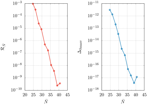
Figure 6: Convergence of the numerical solutions for a localized black hole with inter polar distance $L_{\mathcal{A}}/L\approx 0.00703$. For different resolutions $\bar{N}$ we show the maximal difference $\mathcal{R}_{\bar{N}}$ to a reference solution with high resolution (left) and the deviation from Smarr’s relation $\Delta_{\text{Smarr}}=|(D-2)\tilde{T}\tilde{S}-(D-3-n)\tilde{M}|$ (right). The mean resolution $\bar{N}$ is averaged over all domains and directions.

Finally, we note that the maximum of the non-trivial components of the DeTurck vector $\xi$, cf. equation (18), always remained below $10^{-10}$ for all solutions we constructed.

A.4 Obtaining the phase transition

In order to obtain a highly-accurate value for the position of the first order phase transition, we have to find the intersection point of the localized and the uniform branch in the phase diagrams, cf. figure 1 and figure 4. For this purpose, we compute a series of localized black hole solutions with values of the control parameter $\kappa$ that are distributed on a Lobatto grid around the intersection, i.e. for

$$\kappa_{j} =\frac{\kappa_{\textrm{end}}+\kappa_{\textrm{start}}}{2}-\frac{\kappa_{\textrm{end}}-\kappa_{\textrm{start}}}{2}\cos\left(\frac{\pi j}{N_{\kappa}}\right)\,,\quad j=0,\ldots,N_{\kappa}\,.$$ (20)

An interval $\kappa\in\left[\kappa_{\text{start}},\kappa_{\text{end}}\right]$ in which the corresponding phase transition is located can be easily identified once the data for producing the phase diagrams is at hand. We took $\kappa_{\text{start}}=0.98$ and $\kappa_{\text{end}}=1.02$ (recall that we set $L=8$ in our computations). At each of the Lobatto points we calculate the relevant physical quantities (mass and entropy). By using standard pseudo-spectral techniques we are able to express these quantities in the given interval as a truncated Chebyshev series depending on $\kappa$ with expansion order $N_{\kappa}$. Finally, we identify the phase transition point by determining the root of the difference of these functions and the analytically known uniform branch.

Due to the high accuracy of our localized black hole solutions this procedure will give highly accurate values for the intersection points as well, at least if the resolution $N_{\kappa}$ is high enough, but since we chose a rather small interval $[\kappa_{\text{start}},\kappa_{\text{end}}]$, comparably small values of $N_{\kappa}$ suffice. Moreover, this approach provides a natural estimation of accuracy for the phase transition values, simply by comparing the values obtained for different resolutions, similarly to the procedure described above. The result of this convergence analysis is shown in figure 7.

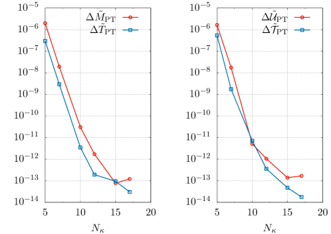
Figure 7: Convergence of the numerically obtained values of the first order phase transition between the localized and the uniform phase. We show the differences to the values of the regarding quantity obtained with $N_{\kappa}=20$ Lobatto points normalized by this value.

Moreover, this procedure even gives a straightforward way to calculate derivatives of the thermodynamic quantities in the corresponding interval $\left[\kappa_{\text{start}},\kappa_{\text{end}}\right]$ by using standard spectral algorithms, which can be employed for obtaining the latent heat, cf. equation (14b). Besides that, we are able to check the first law of thermodynamics $\mathrm{d}M=T\,\mathrm{d}S$ in this interval as an additional consistency check of the numerical results. Indeed, the deviation from this law rapidly drops down as the resolution is increased and saturates at values of $10^{-12}$.

Appendix B Review: $\mathcal{N}=(8,8)$ SYM on $\mathbb{S}^{1}$ and its supergravity description

Strongly coupled $\mathcal{N}=(8,8)$ SYM in the large-N limit is conjectured to be equivalent to type II superstring theory, with string length $l_{s}=\sqrt{\alpha^{\prime}}$ and string coupling constant $g_{s}$.

As discussed in [28, 29], this duality may be motivated within string theory by considering $N$ coincident (non-extremal) D1-branes in type IIB superstring theory. This duality becomes tractable in the limit $1\ll\lambda\ll N^{4/7}$ which we assume to hold from now on. In this regime, curvature scales are much larger than the string scale and the effective string coupling constant is small. Hence, we can approximate superstring theory by type IIB supergravity, and the $N$ coincident D1-branes correspond to a particular (non-extremal) supergravity solution, known as a 1-brane. Finally, taking the decoupling limit

$$l_{s}\rightarrow 0\quad\textrm{with}\ \ g_{s}l_{s}^{-2}\ \ \text{and}\ \ r/l_{s}^{2}\ \ \text{fixed}\,,$$ (21)

we arrive at the conjectured duality between $\mathcal{N}=(8,8)$ SYM and type IIB supergravity. Since we also keep $r/l_{s}^{2}$ fixed, where $r$ represents any physical length, we effectively zoom into the near-horizon part of the supergravity solution.

In addition, to describe $\mathcal{N}=(8,8)$ SYM on a circle $\mathbb{S}^{1}$, the spatial coordinate of D1-branes has to be compactified on a circle with circumference $L$. Due to the compactified spatial direction we have to ensure that the curvature scale has to be small enough such that stringy excitations winding around the $\mathbb{S}^{1}$ are suppressed. In addition, momentum carrying excitations along the circle should not excite string oscillations. In the large $N$ limit and strong coupling limit, this is ensured if $\lambda^{-1/6}\ll\mathcal{T}\ll\sqrt{\lambda}.$ Here $\mathcal{T}$ is the dimensionless temperature associated with the type IIB supergravity solution and may be identified with the dimensionless temperature on the field theory side.

Note that the type IIB supergravity solution breaks down for small enough temperatures. However, for temperatures of order $\lambda^{-1/6}$ or below, we may perform a T-duality along the compactified spatial direction of the type IIB supergravity solution by using the Buscher rules [28, 30]. In particular, the T-duality transforms the length of the circle $L$ into $\tilde{L}=4\pi^{2}l_{s}^{2}/L.$ The resulting type IIA supergravity solution is valid for dimensionless temperatures $\mathcal{T}\ll\lambda^{-1/6}$.

In this paper, we are only interested in the type IIA supergravity description. This supergravity solution may be viewed as D0-branes uniformly smeared along the spatial circle $\mathbb{S}^{1}.$ However, for low enough temperatures, the D0-branes tend to be non-uniformly smeared along this direction. This instability is reminiscent of the well-known Gregory-Laflamme instability in asymptotically flat Kaluza-Klein geometries and was found in [30]. In particular, the onset of the instability occurs for [1, 30, 12]

$$\mathcal{\tilde{T}}_{\text{GL}}=\mathcal{T}_{\text{GL}}\,\sqrt{\lambda}\approx 2.243\,.$$ (22)

In [12], the authors construct the associated non-uniform black string solutions. It is expected that these non-uniform black string solutions with horizon topology $\mathbb{S}^{1}\times\mathbb{S}^{7}$ will merge into the localized black holes with horizon topology $\mathbb{S}^{8}$. The latter ones correspond to D0-branes localized on the spatial circle $\mathbb{S}^{1}.$

References

- [1] R. Gregory and R. Laflamme, “Black strings and p-branes are unstable,” Phys. Rev. Lett. 70 (1993) 2837–2840, hep-th/9301052.
- [2] R. Gregory and R. Laflamme, “The Instability of charged black strings and p-branes,” Nucl. Phys. B428 (1994) 399–434, hep-th/9404071.
- [3] S. S. Gubser, “On nonuniform black branes,” Class. Quant. Grav. 19 (2002) 4825–4844, hep-th/0110193.
- [4] T. Wiseman, “Static axisymmetric vacuum solutions and nonuniform black strings,” Class. Quant. Grav. 20 (2003) 1137–1176, hep-th/0209051.
- [5] E. Sorkin, “A Critical dimension in the black string phase transition,” Phys. Rev. Lett. 93 (2004) 031601, hep-th/0402216.
- [6] B. Kleihaus, J. Kunz, and E. Radu, “New nonuniform black string solutions,” JHEP 06 (2006) 016, hep-th/0603119.
- [7] E. Sorkin, “Non-uniform black strings in various dimensions,” Phys. Rev. D74 (2006) 104027, gr-qc/0608115.
- [8] M. Headrick, S. Kitchen, and T. Wiseman, “A New approach to static numerical relativity, and its application to Kaluza-Klein black holes,” Class. Quant. Grav. 27 (2010) 035002, 0905.1822.
- [9] P. Figueras, K. Murata, and H. S. Reall, “Stable non-uniform black strings below the critical dimension,” JHEP 11 (2012) 071, 1209.1981.
- [10] M. Kalisch and M. Ansorg, “Highly Deformed Non-uniform Black Strings in Six Dimensions,” in Proceedings, 14th Marcel Grossmann Meeting on Recent Developments in Theoretical and Experimental General Relativity, Astrophysics, and Relativistic Field Theories (MG14) (In 4 Volumes): Rome, Italy, July 12-18, 2015, vol. 2, pp. 1799–1804. 2017. 1509.03083.
- [11] M. Kalisch and M. Ansorg, “Pseudo-spectral construction of non-uniform black string solutions in five and six spacetime dimensions,” Class. Quant. Grav. 33 (2016), no. 21, 215005, 1607.03099.
- [12] O. J. C. Dias, J. E. Santos, and B. Way, “Localised and nonuniform thermal states of super-Yang-Mills on a circle,” JHEP 06 (2017) 029, 1702.07718.
- [13] R. C. Myers, “Higher Dimensional Black Holes in Compactified Space-times,” Phys. Rev. D35 (1987) 455.
- [14] T. Harmark, “Small black holes on cylinders,” Phys. Rev. D69 (2004) 104015, hep-th/0310259.
- [15] D. Gorbonos and B. Kol, “A Dialogue of multipoles: Matched asymptotic expansion for caged black holes,” JHEP 06 (2004) 053, hep-th/0406002.
- [16] D. Gorbonos and B. Kol, “Matched asymptotic expansion for caged black holes: Regularization of the post-Newtonian order,” Class. Quant. Grav. 22 (2005) 3935–3960, hep-th/0505009.
- [17] T. Wiseman, “From black strings to black holes,” Class. Quant. Grav. 20 (2003) 1177–1186, hep-th/0211028.
- [18] E. Sorkin, B. Kol, and T. Piran, “Caged black holes: Black holes in compactified space-times. 2. 5-d numerical implementation,” Phys. Rev. D69 (2004) 064032, hep-th/0310096.
- [19] H. Kudoh and T. Wiseman, “Properties of Kaluza-Klein black holes,” Prog. Theor. Phys. 111 (2004) 475–507, hep-th/0310104.
- [20] H. Kudoh and T. Wiseman, “Connecting black holes and black strings,” Phys. Rev. Lett. 94 (2005) 161102, hep-th/0409111.
- [21] M. Kalisch, S. Möckel, and M. Ammon, “Critical behavior of the black hole/black string transition,” JHEP 08 (2017) 049, 1706.02323.
- [22] B. Kol, “The Phase transition between caged black holes and black strings: A Review,” Phys. Rept. 422 (2006) 119–165, hep-th/0411240.
- [23] T. Harmark and N. A. Obers, “Phases of Kaluza-Klein black holes: A Brief review,” hep-th/0503020.
- [24] G. T. Horowitz and T. Wiseman, “General black holes in Kaluza-Klein theory,” in Black holes in higher dimensions, G. T. Horowitz, ed. Cambridge University Press, Cambridge, UK, 2012. 1107.5563.
- [25] M. Kalisch, Numerical construction and critical behavior of Kaluza-Klein black holes. PhD thesis, Jena U., 2018. 1802.06596.
- [26] B. Kol, “Topology change in general relativity, and the black hole black string transition,” JHEP 10 (2005) 049, hep-th/0206220.
- [27] B. Kol, “Choptuik scaling and the merger transition,” JHEP 10 (2006) 017, hep-th/0502033.
- [28] N. Itzhaki, J. M. Maldacena, J. Sonnenschein, and S. Yankielowicz, “Supergravity and the large N limit of theories with sixteen supercharges,” Phys. Rev. D58 (1998) 046004, hep-th/9802042.
- [29] M. Ammon and J. Erdmenger, Gauge/gravity duality. Cambridge University Press, 2015.
- [30] O. Aharony, J. Marsano, S. Minwalla, and T. Wiseman, “Black hole-black string phase transitions in thermal 1+1 dimensional supersymmetric Yang-Mills theory on a circle,” Class. Quant. Grav. 21 (2004) 5169–5192, hep-th/0406210.
- [31] T. Harmark and N. A. Obers, “New phases of near-extremal branes on a circle,” JHEP 09 (2004) 022, hep-th/0407094.
- [32] S. Catterall, A. Joseph, and T. Wiseman, “Thermal phases of D1-branes on a circle from lattice super Yang-Mills,” JHEP 12 (2010) 022, 1008.4964.
- [33] S. Catterall, R. G. Jha, D. Schaich, and T. Wiseman, “Testing holography using lattice super-Yang-Mills theory on a 2-torus,” Phys. Rev. D97 (2018), no. 8, 086020, 1709.07025.
- [34] R. G. Jha, S. Catterall, D. Schaich, and T. Wiseman, “Testing the holographic principle using lattice simulations,” EPJ Web Conf. 175 (2018) 08004, 1710.06398.
- [35] B. Cardona and P. Figueras, “Critical Kaluza-Klein black holes and black strings in D=10,” to appear.
- [36] R. Emparan, R. Luna, M. Martinez, R. Suzuki, and K. Tanabe, “Phases and Stability of Non-Uniform Black Strings,” 1802.08191.
- [37] T. Wiseman, “Numerical construction of static and stationary black holes,” in Black holes in higher dimensions, G. T. Horowitz, ed. Cambridge University Press, Cambridge, UK, 2012. 1107.5513.
- [38] O. J. C. Dias, J. E. Santos, and B. Way, “Numerical Methods for Finding Stationary Gravitational Solutions,” Class. Quant. Grav. 33 (2016), no. 13, 133001, 1510.02804.
- [39] P. Figueras, J. Lucietti, and T. Wiseman, “Ricci solitons, Ricci flow, and strongly coupled CFT in the Schwarzschild Unruh or Boulware vacua,” Class. Quant. Grav. 28 (2011) 215018, 1104.4489.
- [40] B. Kol, E. Sorkin, and T. Piran, “Caged black holes: Black holes in compactified space-times. 1. Theory,” Phys. Rev. D69 (2004) 064031, hep-th/0309190.
- [41] T. Harmark and N. A. Obers, “New phase diagram for black holes and strings on cylinders,” Class. Quant. Grav. 21 (2004) 1709, hep-th/0309116.