Tuning of MC generator MPI models

Abstract

Contributed chapter to “Multiple Parton Interactions at the LHC”, World Scientific
MC models of multiple partonic scattering inevitably introduce many free parameters, either fundamental to the models or from their integration with MC treatments of primary-scattering evolution. This non-perturbative and non-factorisable physics in particular cannot currently be constrained from theoretical principles, and hence parameter optimisation against experimental data is required. This process is commonly referred to as MC tuning. We summarise the principles, problems and history of MC tuning, and the still-evolving modern approach to both model optimisation and estimation of modelling uncertainties.

1 Introduction

It is an unfortunate fact of life that the modelling approaches to multiple partonic scattering implemented in Monte Carlo event generator programs are not fully unambiguous. Not only are ansätze required for computation of the hadronic matter overlap and low-$p_{\perp}$ regularisation of the partonic scattering cross-section, but also the secondary scattering must coherently connect to the other aspects of event modelling in general-purpose MC codes.

For example, MPI scattering must interface somehow with QCD evolution down to soft momentum-transfer scales, as described by parton showers and matrix element corrections, and to the colour connections between the partonic scattering system and the beam remnants. Phenomenological hadronisation models must also be modified to accommodate MPI as a source of partons, most notably via somewhat ad hoc “colour reconnection” or “colour disruption” mechanisms.

The result of this complexity is that MPI models not only contain degrees of freedom intrinsic to their own formulation, but also require extensions to the generator components concerned with the primary partonic scatter. As much of the physics involved is non-perturbative — and that which is not is only defined up to leading-order or leading-logarithmic accuracy — it is typical for more than ten model parameters to influence observables of interest, with little or no a priori prediction of their values. These parameters must somehow be “tuned” to describe MPI-sensitive observables in experimental data.

In this chapter we describe the dominant modern approach to MC generator parameter optimisation, from the technical machinery to the parameters and observables, and the methodology applied to both achieve convergence and avoid overfitting. As is always true for parameter estimation in physics, the resulting uncertainty is as important as the central value and hence we review the statistical methodology applied to estimate model uncertainties through tuning. Finally, we survey the road ahead for MC tuning and improved constraints on MPI modelling.

2 Tuning methodology

From the outset we should be clear that tuning is not desirable. While currently a necessary part of the landscape of MPI modelling (and other hadron-collider event features), in an ideal world our models would have sufficiently few ambiguities that tuning will become unnecessary. We can dream! But for now, modelling flexibility is necessary to achieve the degree of data description required by experiment — at the significant cost of exchanging parameter fitting and uncertainty estimation for predictivity.

In this pragmatic compromise, it is preferable not to simply throw all possible parameters and data into a massive fit. Rather, well-motivated modelling components — typically those involving QCD at perturbative scales — are trusted to be predictive from first principles, while phenomenological models which are only unconstrained in the asymptotic limits of QCD are ripe for fitting. We use the word “tuning” to refer only to fits of the latter parameter type, and as far as possible avoid fitting true theory uncertainties such as scale choices in the perturbation expansion.

In the simplest case, tuning consists of finding the value of a single model parameter — say, the $p_{\perp}$ scale used to regularise the divergent secondary scattering cross-section — which gives the best agreement with a single data bin, e.g. a total cross-section for double-partonic scattering. For this, little technical machinery is required: a set of MC generator runs with different values of the parameter (either over the whole natural range of the model, or focused on a “known-good” region) are compared to the data, and the best-performing model point is chosen as the “tune”. Perhaps a couple of iterations will be required. This is “manual tuning.”

Extension of this scheme to include more data is simple but not entirely trivial. For example, a multi-bin observable such as an “underlying event” characterisation of mean particle or energy flow away from the hard primary scattering products, simply requires that the goodness of fit be computed via an aggregation of the fit quality across the many bins. Computing the fit quality naturally introduces several questions:

1. Which regions of the observable are most important to describe?

2. Are there bins which the model fundamentally can/should not describe?

3. Are these bins independent of each other, or correlated somehow?

Unfortunately we do not have general answers to the first two of these points, which immediately makes a robust statistical foundation for tuning problematic. The third in principle can be solved by publication of bin-correlation data, but this has both been rare in MPI-sensitive measurements until now, and is arguably rendered moot by the first two issues. We shall return to this theme later.

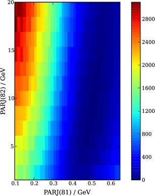
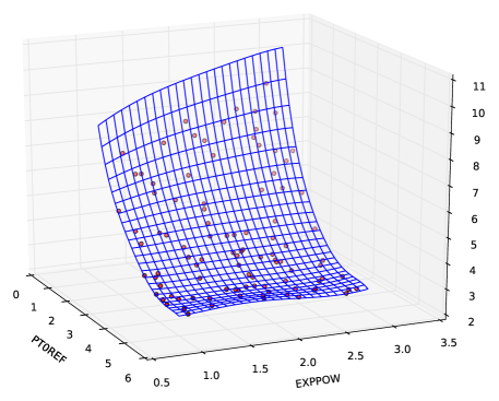
Figure 1: Goodness-of-fit characterisations in 2-parameter tunes. Left, LEP event thrust in Pythia 6 parton shower; Right, LHC minimum-bias in Pythia 8 MPI model (with Professor $\chi^{2}$ function fit to the sampled points).

Now a more technically troublesome extension: more parameters. In a two-dimensional parameter space, such as including a scaling parameter for the hadronic matter distribution in addition to the $p_{\perp}$ regulariser — a by-eye approach is still possible: as before, make MC runs for several combinations of the two parameters’ values and compare to data. In addition, computing a goodness-of-fit measure for all points in a 2D grid can provide a useful visualisation of the physics dependence, as illustrated in Figure 1. But the increased computational cost is clear: if $N$ trial points were required for a single parameter, $\mathcal{O}(N^{2})$ will be required for two parameters, and this exponential scaling continues into the less visualisable spaces of 3 and more parameters. The severity of this problem is emphasised by the expense of a typical parameter-point evaluation: the required statistical precision means that $\mathcal{O}(\text{100k--1M})$ events are needed per colliding-beam configuration and per primary-scattering process type, hence the total time for a parameter point may be counted in CPU-days. A comprehensive grid-scan of the $\mathcal{O}(\text{10--20})$ parameters needed in a full generator is clearly unfeasible.

One possible approach is physical intuition, and this is undoubtedly helpful. Fortunately a 20-dimensional appreciation of model behaviour is not necessary, since many modelling components approximately factorise and can be reasoned about in isolation. But even so, once more than a few interconnected parameters are involved, intuition is not enough to break fit-quality degeneracies, and it is impossible to be sure that a final intuitive tune is truly optimal. However, despite the availability of more technical machinery, the wholly intuitive approach is far from irrelevant [1].

The alternative is to somehow make do with an incomplete sampling of the parameter space, and to use computational machinery to guide the fit. Done naïvely, this runs into problems of its own: a random sampling of a large-dimensional space gives little confidence that the best-seen parameter point is anywhere near to the global optimum. Attempting to systematically improve on the points visited so far would provide a better sampling of the space, but at the unsustainable cost of abandoning the implicitly parallelisable approach of independent MC runs. Even very sophisticated attempts to serially sample MPI model parameter spaces have proven intractable due to the high computational cost of the MC “function” [2]. Instead, the method which has become most widespread, via the Professor toolkit [3], is a hybrid of parallel sampling and serial optimisation, via parametrisation of the MC generator response to parameter variations. It is this approach to which we will dedicate most space in this summary. First, however, it is important that we acquaint ourselves with the typical parameters and observables that will be encountered while constructing an MC generator tune.

2.1 Experimental observables and model parameters

While our interest here is naturally biased toward the MPI-specific aspects of generator modelling, it is worthwhile to also discuss how the rest of the generator system is involved in tuning. In rough reverse order from final to initial state, the main components of an MC generator are hadronisation, fragmentation, final-state QCD radiation, initial-state QCD radiation, and multiple partonic scattering. Taken together, these components readily comprise a parameter space with in excess of 30 dimensions. Even with computational tricks in the generator runs, sampling such a space requires extraordinary CPU resources. But there are usually significant factorisations between these major modelling steps, which can be exploited to make the tuning more tractable.

Typically we start by identifying these factorised blocks working backward from the final state, assuming that decays, hadronisation (not including colour reconnection), and the final-state parton shower should be sufficiently independent of initial-state QCD effects that they can be tuned to $e^{+}e^{-}$ data from LEP and SLD only. Using hadron collider data (at least in the first iteration) could bias this tuning via poor initial-state modelling, so it is typically left out, saving CPU time and complexity. Since hadronisation models can account for the majority of MC generator parameters, it is not unusual to split this final-state tuning stage into several rounds, e.g. first concentrating on using identified hadron rates [4] to fix hadronisation parameters such as strangeness suppression, then using identified particle energy spectra, event shapes, and jet rates [5, 6, 7] to constrain the final-state parton shower and fragmentation functions. As the parton shower is built on perturbative physics, it has few degrees of freedom: typically just the emission cutoff scale and perhaps the definition of $\alpha_{\text{S}}$ evolution. Treated in this combined way, the first Professor tunes of Pythia 6 achieved degrees of data description for LEP event shapes, jet rates, and $b$-fragmentation that had previously eluded manual tunes.

Having addressed the tuning of final-state modelling, we now confront the combination of the initial-state parton shower, the MPI mechanism, and the colour-reconnection mechanism: all key to description of particle production and energy flow observables at hadron colliders. The most important observables depend on the bias of one’s physics interest, but in the general-purpose tunes which have received most attention, the emphasis in soft QCD has been on kinematics rather than flavour content. This due to experimental priorities: for most purposes at the LHC, secondary-scattering is a background to measurement of hard signal-process scattering, and hence the key requirement of a general-purpose MPI tune is to accurately model its contribution to charged track multiplicities and energy flows. Since these background contributions are divided into inclusive soft-QCD scattering in additional $pp$ collisions (known as “pile-up”), and additional partonic scattering in signal events (the “underlying event”), the dominant observables in such tunes are those measured in inclusive “minimum bias” event selection, and those specific to the underlying event.

Minimum-bias physics measurements at hadron colliders have been dominated by charged-track observables, partially because the low-luminosity early phases of each data-taking run are crucial for calibration of detector tracking systems. The main data from these measurements, often grouped as “min-bias observables”, are charged-particle multiplicities and $p_{\perp}$ spectra within fiducial acceptance cuts (most obviously the tracker coverage in pseudorapidity, $\eta$), and the correlation of the average charged-particle $p_{\perp}$ with the event’s fiducial track multiplicity. Broadly speaking, the distribution of charged-particle multiplicity $N_{\mathrm{ch}}$ with $\eta$ is the canonical distribution used to indicate the inclusive amount of minimum bias particle production, particularly in the flat central region $|\eta|<1$. This is governed by a correlated combination of MPI $p_{\perp}^{0}$ regularisation parameter, the amount of hadronic matter overlap for large impact parameter (since $b\sim 1/Q$ and the typical scale $Q$ of inclusive minimum-bias interaction is low), and perhaps scaling of the MPI partonic process via freedom in parametrisation of the MPI $\alpha_{\text{S}}$. The correlation of $\langle p_{\perp}\rangle$ with $N_{\mathrm{ch}}$ became an important tuning observable when it was noted that models without colour-reconnection were unable to describe it, predicting too soft a particle production spectrum in higher-multiplicity scattering events. Colour disruption mechanisms were added to the hadronisation models of Pythia and Herwig to address this, naturally introducing extra degrees of freedom for tuning.

In the LHC era, additional fiducial cuts were introduced to minimum-bias data analyses as variations of “analysis phase space” to modify the sensitivity to different aspects of inclusive scattering physics. These include requirements on charged-particle fiducial multiplicity (e.g. from 1 to $\sim\!20$) and on minimum charged-particle $p_{\perp}$ (e.g. from 100 MeV to $\sim\!\!10$ GeV). The result is that a very large number of many-bin observables, generally with small uncertainties, is available from the Tevatron to the LHC, and from 300 GeV to 13 TeV beam energies [8, 9, 10, 11, 12, 13, 14, 15, 16, 17]. In addition, ATLAS and CMS have published calorimetric measurements of energy flow as a function of $\eta$, including a minimum-bias trigger selection. These provide a counterpart to the track-specific measurements, including both a central overlap with tracking detector acceptance and extension to high-$|\eta|$, crucial for forward/diffractive and beam-connection physics. This availability of multiple independent measurements of each observable is important to avoid overfitting of a single measurement, and the different phase spaces enable, for example, degeneracy breaking between non-diffractive MPI and diffractive physics contributions to particle production.

Underlying event (UE) analyses are a specialisation of the minimum bias observables to events where a more exclusive trigger is required, i.e. a genuinely high-scale scattering process such as hard jet or $Z$ boson production. Typically the motivation of UE measurements is to specifically study the connection between this hard process and the associated secondary scattering, as a test of the eikonal MPI model and of the interaction between it and the perturbative QCD dressing of the primary scatter.

Since a hard primary partonic process will dominate the particle- and energy-flow characteristics of each event, UE analyses specifically analyse event regions expected to contain minimal hard process contamination — for example, regions azimuthally transverse to the axis of a balanced dijet event [18, 19, 20], transverse to or in the direction of a hard leptonic $Z$ [21, 22], or with identified jet activity “cut out” from anywhere in the event $\eta$–$\phi$ phase space [23]. The transverse regions are often further specialised to discriminate between the more and less active sides on a per-event basis, to provide additional resolution between MPI and parton shower activity.

The canonical UE observable is the evolution of the mean value of a minimum-bias event property like charged-particle multiplicity or $p_{\perp}$ sum within a sensitive phase-space region, as a function of the scale (usually a $p_{\perp}$) of the hard scattering process. This produces an extremely informative curve showing the smooth evolution of mean event properties from minimum-bias at low event scales (interpreted as peripheral hadronic collisions), up to very hard primary scatterings as $b\to 0$. Underlying event physics hence probes the same MPI mechanisms as minimum-bias (particularly high-activity MB phases spaces), but with a clear connection to the pedestal effect, which maps the matter overlap profile in detail, and an increased emphasis on the role of initial-state QCD radiation from the high-scale primary process.

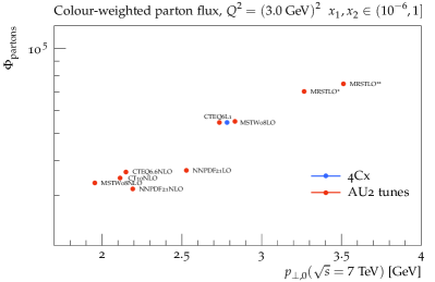
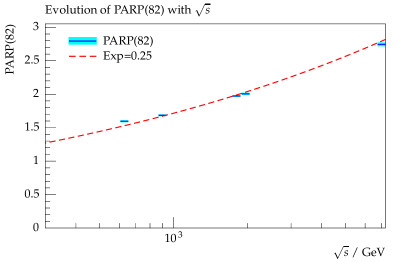
Figure 2: 2 Tuned Pythia 8 MPI cross-section regulariser, $p_{\perp}^{0}$, as a function of low-$x$ gluon luminosity from various PDFs. The correlation between higher gluon flux and higher $p_{\perp}^{0}$ (meaning more screening of that flux) is clear. 2 Empirical $p_{\perp}^{0}$ scaling via independent tunes to hadron collider data at different $\sqrt{s}$.

Parton density functions play an important role in hadronic initial-state tuning, particularly MPI since the partonic cross-section for multiple scattering at low-$Q$ is strongly driven by the diverging low-$x$ gluon PDF, which varies a great deal between different PDF fits. Additionally, PDF differences produce variations in the rapidity distribution of MPI partonic scattering. These effects, influencing the multiplicity of MPI scattering and $d\eta/dN_{\mathrm{ch}}$ distribution shapes respectively, are responded to in tuning by correlated shifts in the $p_{\perp}^{0}$ screening factor, matter distribution/overlap parametrisation, and MPI $\alpha_{\text{S}}$. The Pythia MPI model in particular is rather over-parametrised: the MPI rate can be more-or-less directly modified via $p_{\perp}^{0}$, $\alpha_{\text{S}}$, and a partonic scattering scale-factor. Naïvely throwing all these parameters into a fit will likely produce degenerate or overfitted tunes: it is best to instead use a subset of at most 3 parameters, e.g. $\alpha_{\text{S}}$ or scale-factor (or neither) but certainly not both in a single tune. The relationship between gluon luminosity (the integral of a PDF over MPI partonic scattering scales) and tuned $p_{\perp}^{0}$ may be seen in Figure 2: a more divergent low-$x$ PDF with a higher gluon luminosity is strongly correlated with a higher $p_{\perp}^{0}$ tune value and hence more screening of the divergence. Tunes, or at least their MPI component, are hence specific to a particular PDF — even, arguably, to the variation fits within a given PDF set.

A key aspect of MPI tuning in modern MC generators is to fit the $\sqrt{s}$ dependence of the model. The Jimmy MPI model, and early versions of Herwig++, attempted to describe all MPI activity with a fixed $p_{\perp}$ regulariser value at all energies, but this ultimately proved unworkable and a Pythia-like $\sqrt{s}$ dependence with a slow power-law dependence similar to total $pp$ cross-section fits [25] was instead introduced. The analogy is not predictive, however, so this exponent is also a free tuning parameter for any tune interested in describing more than one collider energy. Experimental data from more than one energy is obviously needed to constrain this parameter, but the power-law ansatz has been found to work well and even been supported empirically by independent tunes of $p_{\perp}^{0}$ at different $\sqrt{s}$  [26] as shown in Figure 2.

Finally, a marginal aspect of tuning: the “primordial $k_{\perp}$”. This quantity, implemented in several parton shower generators, is the $\mathcal{O}(1)~{}\text{Ge\kern-0.6458ptV}$ width of a function used to add a randomly sampled transverse momentum boost to the whole modelled scattering event. This is motivated almost entirely by the pragmatic desire for a good description of the $Z$ $p_{\perp}$ differential cross-section, a precisely measured observable generated by initial-state recoils, which rises steeply from zero at $p_{\perp}(Z)=0$ to a peak at a few GeV. The exact position of this peak is determined by resummation of large QCD logarithms, i.e. the process approximated by the parton shower. Comparisons to data with a “vanilla” parton shower almost invariably produce a peak at too small a $p_{\perp}$ value, and hence primordial $k_{\perp}$ smearing was introduced as the simplest possible mechanism to “correct” this flaw in data description. While this nebulous shortcoming of parton shower models is somewhat distressing, at present only the $Z$ $p_{\perp}$ distribution is precisely enough measured at hadron colliders to be sensitive to this effect (and other very soft QCD modelling effects, such as the ISR shower cutoff scale and/or Powheg real emission cutoff [27]). Primordial $k_{\perp}$ can hence be tuned virtually independently of other initial-state quantities, although it can equally be included in larger tunes, where it becomes a flat direction in the parameter space for all bins except those in the low-$p_{\perp}$ region of $Z$ $p_{\perp}$ and related observables.

2.2 Parameterisation-based tunes:

Tuning via parametrisation of MC generator behaviour has a lengthy history [28, 29, 30, 6, 31, 5]. The fundamental idea is to replace the expensive, probably multi-day, explicit evaluation of a proposed MC parameter point with a very fast, analytic approximation.

It is tempting to try to parametrise the shape of an observable as a whole as function of some input parameters by using splines or similar structures. This, however, is a non-trivial task as the functional form of an observable will in most cases not be parametrisable by simple functions. Similarly, parametrising the entirety of a multi-bin goodness-of-fit (GoF) function proves fraught. Instead, a $P$-dimensional polynomial is independently fitted to the generator response, $\text{MC}_{b}(\mathbf{p}=(p_{1},\dots,p_{P}))$, of each observable bin $b$. By doing so the potentially complicated behaviour of observables is captured by a collection of simple analytical functions.

Having determined, via means yet undetailed, a good parametrisation of the generator response to the steering parameters for each observable bin, it remains to construct a GoF function and minimise it. The result is a predicted parameter vector, $\mathbf{p}_{\text{tune}}$, which should (modulo checks of the technique’s robustness) closely resemble the best description of the tune data that the generator can provide.

In parametrisation-based tuning, the run-time is dominated by the time taken to run the generator to produce inputs to the parameterisation. This step is trivially parallelisable and large tunes can be tractable even with modest computing resources. The calculation of the parameterisation rarely exceeds a few minutes, as does the subsequent numerical minimisation step: this technique hence enables rapid tuning in response to new measurements, as well as systematic exploration of freedoms in the tuning procedure itself. The preparation of input data depends on the complexity of the task at hand, namely the sophistication of the generator and the dimension of the parameter space.

It is important to check the fidelity of the parametrisation, and to ensure that the parametrisation scan includes predictions surrounding the target data values. The construction of “envelope plots” is a good practice to check a priori that the chosen sampling range actually covers the data considered for tuning. For each bin of each observable the minimal and maximal value from the corresponding inputs is obtained and thus allows to spot mistakes and model limitations early on, as shown in Figure 3. Using disjoint sets of input MC data for parametrisation-building and testing allows the accuracy of the parametrisation to be estimated.

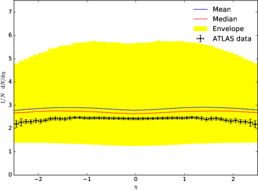
Figure 3: Example of a tuning “envelope plot”. Here the experimental data is clearly contained within the yellow band of the sampled model space, but that is not always the case.

Fitting model

To illustrate the method, we discuss the parameterisation of the bin content $\text{MC}_{b}$ using a general polynomial of second order:

$$\text{MC}_{b}(\mathbf{p})\approx\alpha^{(b)}_{0}+\sum_{i}\beta^{(b)}_{i}\,p^{\prime}_{i}+\sum_{i\leq j}\gamma^{(b)}_{ij}\,p^{\prime}_{i}\,p^{\prime}_{j}.$$ (1)

The task at hand is to determine the coefficients $\alpha,\beta_{i},\gamma_{i}$. Algorithmically this is done by generating at least as many inputs $\text{MC}_{b}(\mathbf{p})$ for different $\mathbf{p}$ as there are coefficients in the to be fit polynomial such that we are able to solve a system of linear equations. Since it is much more practical we cast the right hand side into a scalar product:

$$\text{MC}_{b}(\mathbf{p})\approx f^{(b)}(\mathbf{p})=\sum_{i=1}^{N_{\text{min}}(P)}c^{(b)}_{i}\,\tilde{p}_{i}.$$ (2)

For a second order polynomial of a two dimensional parameter space ($x,y$), the coefficient vector would have the form

$$\mathbf{c^{(b)}}=(\alpha,\beta_{x},\beta_{y},\gamma_{xx},\gamma_{xy},\gamma_{yy}),$$ (3)

and for each set of input points ($x_{i},y_{i}$) we can write

$$\tilde{p}_{i}=(1,x_{i},y_{i},x_{i}^{2},x_{i}y_{i},y_{i}^{2}).$$ (4)

By doing so and denoting the set of $\tilde{p}_{i}$ as $\tilde{P}$ and the set of corresponding bin values as $\mathbf{\text{MC}_{b}}$ we construct the matrix equation

$$\text{$\mathbf{MC}$}_{b}=\mathbf{\tilde{P}}\cdot\mathbf{c^{(b)}},$$ (5)

which allows us to determine the set of coefficients $\mathbf{c^{(b)}}$ by inverting $\mathbf{\tilde{P}}$, i.e.

$$\mathbf{c^{(b)}}=\mathcal{I}[\tilde{P}]\mathbf{\text{MC}_{b}}.$$ (6)

In Professor, a singular value decomposition (SVD) algorithm (implemented in the Eigen3 library) is used to perform the matrix (pseudo)inversion $\mathcal{I}[\tilde{P}]$. The SVD method is equivalent to a desirable least-squares fit of the target polynomial to the input data. In the case of having as many input points as there are coefficients to be determined, the solution is exact. When providing more than $N_{n}(P)$ inputs, the system is over-constrained and therefore the fit will average out to some degree both statistical fluctuations and the fact that the true generator response will almost never be fully describable by a general polynomial. We prefer to oversample by at least a factor of two for robustness. As only the central bin values enter the SVD algorithm, but the statistical uncertainty of the input data is crucial to GoF construction and optimisation, the bin uncertainties are fitted as a separate polynomial in exactly the same way as the bin values.

The dimension of the parameter space and the order of the polynomial to be fitted determine the dimension of the to be inverted matrix and thus the minimal number of required input datasets. Generating more inputs than minimally necessary is in this context equivalent to over-constraining a system of linear equations. Doing so has the benefit of being able to test the stability of the obtained best parameter point against two aspects. One being the order of polynomials chosen as higher order correlations can become important. Secondly, although parametrisations obtained from all available inputs should give the best prediction of the generator response in the whole of the parameter space, smaller subsets can yield different best parameter points which is indicative of the polynomial approximation breaking down (typically in a too large parameter space). The number of coefficients of a $P$-dimensional general polynomial of order $n$ is

$$N_{n}(P)=1+\sum_{i=1}^{n}\,\frac{1}{i\,!}\,\prod_{j=0}^{i-1}(P+j).$$ (7)

How the number of parameters scales with $P$ for 2nd and 3rd order polynomials is tabulated in Table 1 and shown in Figure 4. The latter also shows how computational cost scales with $P$ and $n$.

Num params, $P$	$N_{2}(P)$ (2nd order)	$N_{3}(P)$ (3rd order)
1	3	4
2	6	10
4	15	35
8	45	165

Table 1: Scaling of number of polynomial coefficients $N_{n}(P)$ with dimensionality (number of parameters) $P$, for polynomials of second- ($n=2$) and third-order ($n=3$).

Professor allows to calculate polynomials of in principle arbitrary order, including $0$th order, i.e. the constant mean value. To account for lowest-order parameter correlations, a polynomial of at least second-order should be used as the basis for bin parametrisation. In practice, a 3rd order polynomial suffices for almost every MC generator distribution studied to date, i.e. there is no correlated failure of the fitted description across a majority of bins in the vicinity of best generator behaviour. An upper limit on the usable polynomial order is implicitly given by the double precision of the machinery effectively limiting the maximum usable order to about 11. It should be noted that other classes of single polynomials such as Chebychev or Legendre have no additional benefit in the Professor method. The quality of the resulting parametrisation is exactly the same, with merely different groupings of the coefficients.

The set of input points for each bin are determined by randomly sampling the generator from $N$ parameter space points in a $P$-dimensional parameter hypercube $[\,\mathbf{p}_{\text{min}},\mathbf{p}_{\text{max}}]$ defined by the user. This definition requires physics input — each parameter $p_{i}$ should have its upper and lower sampling limits $p_{\text{min,max}}$ chosen so as to encompass all reasonable values while avoiding discontinuities. In cases where bin values vary over many orders of magnitude general polynomials are obviously a poor choice for an approximate function. It is nonetheless possible to use Professor by simply taming the input data by parametrising e.g. the logarithm of bin values.

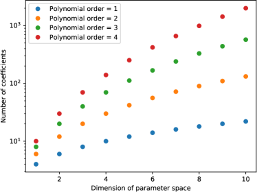
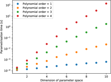
Figure 4: Parameterisation requirements. Left, $N_{n}(P)$ vs $P$; Right, single core computation time vs $P$.

Goodness of fit function and optimisation

With the parameterisation of the generator at hand the optimisation can be turned into a numerical task. By default an ad hoc GoF measure is minimised using Minuit’s migrad algorithm with the typical features of being able to fix or impose limits on individual parameters during the fit. For the purpose of generator tuning with typically imperfect models it is often necessary to bias the GoF in order to force the description of certain key observables, e.g. the plateau of the underlying event or to switch off parts of histograms entirely when it is known that the underlying model is unable to describe the data at all. The relative importance of individual bins and observables can be set in Professor using weights, $w_{b}$, in the GoF definition:

$$\chi^{2}(\mathbf{p})=\sum_{\mathcal{O}}\sum_{b\,\in\,\mathcal{O}}w_{b}\cdot\frac{(f^{(b)}(\mathbf{p})-\mathcal{R}_{b})^{2}}{\Delta^{2}_{b}(\mathbf{p})},$$ (8)

where $\mathcal{R}_{b}$ is the reference data value for bin $b$. The error $\Delta_{b}$ is composed of the total uncertainty of the reference which is a constant for each point $\mathbf{p}$ and the parameterised statistical uncertainty of the Monte Carlo input for bin $b$. In practice we attempt to generate sufficient events at each sampled parameter point that the statistical MC error is much smaller than the reference error for all bins.

Further methods

Optimisation in tuning is by no means limited to this setup. The Python language bindings to the core objects in Professor allow to easily construct arbitrary GoF measures and to use other minimisers that have Python bindings, such as MultiNest [32].

Although being highly successful, the polynomial parameterisations have obvious limitations. The framework hence allows to use different parameterisation methods for instance the ones available in scikit-learn and Gaussian Processes where no prior assumption on the functional form has to be made.

Professor also provides tools for the interactive exploration of the parameter space as GTK application as well as Jupyter notebooks. Both allow to load a previously calculated set of parametrisations and displays the corresponding histograms. GUI sliders (one per parameter) allow to conveniently set the parameter point to a new value resulting in the histogram being redrawn immediately. These tools help to build intuition into what effect parameters have on distributions.

3 Influential MC generator tuning results

Parton shower MC generators have been tuned for as long as they have existed: the intrinsic limitations of their formal accuracy and the dependence of truncated perturbative calculations on unphysical scales means that some authorial intuition has long been needed to achieve a good description of key data observables “out of the box”. At LEP, the experiments also sank effort into tuning of final-state parton showers and fragmentation. But the existence of a wider programme of tuning, particularly for MPI modelling, started with the work of Rick Field and the CDF tunes of Pythia 6 [33].

The first such construction was Tune A, its name acknowledging immediately that it was bound not to be the last word on this limitless subject. Tune A was constructed specifically to provide a first reasonable modelling of the underlying event, based on CDF’s first UE measurement [34]. However, it was soon noticed that its parameter choices, particularly for the PARP(64) parameter governing the ISR evolution scale and the PARP(91) primordial $k_{\perp}$ width, resulted in a $Z$ $p_{\perp}$ spectrum whose peak was at too small a $p_{\perp}$ value. A new tune was needed [33, 35], and soon came in the form of Tune AW with a 2.1 GeV primordial $k_{\perp}$ width and a reduced ISR scale — corresponding to a larger $\alpha_{\text{S}}$ and hence more initial-state radiation against which to recoil. Inevitably, Tune AW also hit an obstacle: the dijet azimuthal decorrelation distribution [36], characterising the extent to which, in generic Tevatron jet events, initial-state recoils between high-$p_{\perp}$ jets push the leading dijet system away from the 2-body back-to-back configuration. Having specifically boosted the amount of ISR to create Tune AW, it now needed to be reduced again (this time via Pythia’s PARP(67) ISR starting scale parameter) to avoid creating too many hard multi-jet events: the resulting tune was christened Tune DW. Several other variations joined the swelling ranks of CDF Pythia 6 tunes, including variations in PDF choice and the energy dependence of MPI regularisation. (This last issue, almost in isolation, was also applied to tuning of the Herwig MPI model, Jimmy, in anticipation of the energy leap from Tevatron to LHC.)

The pattern at this point had become clear: the initial-state system of MPI, ISR, and intrinsic $k_{\perp}$— as well as developments in matrix element matching & merging — was too complex to be entirely optimised by hand. Every single-parameter change would both address the modelling problem at which it was aimed, and break several other distributions. The Professor tuning effort arose at this point, to apply the computational methods described above to this optimisation problem. The first and only tunes to bear the Professor label were the Prof0-Q2 and Prof0-pT tunes [3] of Pythia 6, for its virtuality ordered parton shower and newer $p_{\perp}$-ordered parton shower respectively. Both tunings were “global”, in the senses that they covered all aspects of the generator from final-state showering and hadronisation, to the initial-state effects covered by the CDF tunes as well as the widest available dataset from LEP hadron spectra to event shapes, and to Tevatron minimum-bias and underlying event data. More influentially, the Professor machinery was immediately used within ATLAS to produce its own tune series first based on CDF data and then including the early ATLAS data in the AMBT and AUET tune series between 2009 and 2012. Also influential were the hand-tuned “Perugia” family by Peter Skands, particularly since they included systematic variations of the parton showers useful for uncertainty estimation.

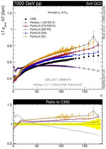
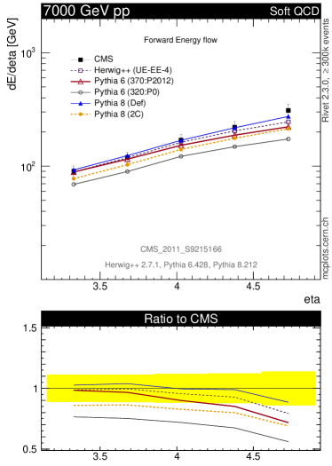
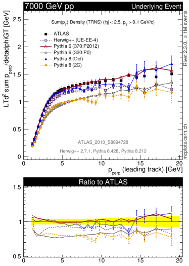
Figure 5: Performance of MC tunes on MPI-sensitive observables, showing Pythia 6 (two “Perugia” tunes), Pythia 8 (the author Tune 2C and default Monash tune), and Herwig++ (UEEE-4 tune). The Perugia 0 and 2C tunes are based on pre-LHC Tevatron data, and the others include early LHC data. The top row shows LHC minimum-bias $p_{\perp}$ spectrum and $\langle p_{\perp}\rangle$ vs. $N_{\mathrm{ch}}$ observables, and the bottom row shows tune performance on minimum-bias energy flow (left), and underlying event $\sum p_{\perp}$ observables. The inclusion of LHC data in all cases improves the data description.

As suggested by the story so far, the initial LHC tuning community focus was concentrated on Pythia 6. Additional work was performed at this time, largely via the Professor technique, to tune the Sherpa fragmentation model and the Jimmy MPI mechanism for the Herwig 6 generator. The next major developments in MPI tuning were the shift during LHC Run 1 to the newer C++ family of generators. The Pythia 8, Herwig++, and Sherpa generators were all tuned using the Professor tools within their development collaborations, with the most notable outputs being the Pythia 8 Tune 4C, and Herwig++’s UEEE tune series which introduced tuned modelling of MPI energy evolution and colour-reconnection in response to the evidence that MPI observables could not be successfully tuned within the existing model space without such mechanisms.

ATLAS and CMS tuning of Pythia continued, with ATLAS’s A1, A2 and AU2 tunes being heavily used in the Run 1 simulation leading up to the Higgs boson discovery, while CMS’ “Z”-tune variants on the AMBT series were used for the same purpose on that experiment. Each experiment focused on its own growing collection of soft-QCD data analyses as the LHC energy increased. At the end of LHC Run 1, Skands and collaborators provided the “Monash” global tunes of Pythia 8 [1], which ATLAS modified into the “A14” tunes for use in Run 2 modelling, incorporating high-$p_{\perp}$ $Z$ and $t\bar{t}$ observables into the fit to serve the needs of BSM searches [37]. CMS, meanwhile, constructed its own Run 2 series, the CUET and CDPST tunes [38], the latter of which is unique in being tuned to hard double-partonic scattering data. At the time of writing, these experiments’ and authors’ tunes of Herwig++ and Sherpa are the most widespread general purpose tunes at the LHC.

Recently most LHC tuning effort has been focused on configurations most suitable for use with matching and merging event generators in which the parton shower is interleaved with collections of higher-order matrix elements. The results have been specialist tunes such as ATLAS’ AZ and AZNLO [39] (specifically for description of the $Z$ $p_{\perp}$, to be used in $W$-mass measurement) and ATTBAR [40]. The LHC split between tunes for minimum-bias data description and underlying-event description has also still to be resolved, perhaps by inclusion of more advanced diffractive physics models although efforts along those lines have yet to prove fully satisfying.

4 Tuning uncertainties

Producing optimal fits of MC models to data is valuable, but not the whole story. In particular for experimentalists’ usage of these simulations, it is crucial that the uncertainties in a tuned model also be quantified. This permits, in varying degrees of sophistication, numerical treatment of modelling uncertainties as nuisance parameters in fits of physics both from the Standard Model and from beyond it. Estimates of tuning uncertainty also proved valuable in the run-up to LHC operations, when tune fits to Tevatron and other low-energy data permitted a quantitative estimate of the range of underlying event activity to be expected at the new 13 TeV collider — this extrapolation of uncertainty is visible in Figure 6.

Simple uncertainty estimates can be produced in various ad hoc ways. First, an approach analogous to scale choices in perturbative calculation: simply pick some parameter variations that seem “reasonable” — typically factors of two — and release them as variation tunes. A step up in sophistication is to make such changes to key parameters, e.g. enforcing more or less initial-state radiation, and then re-tuning the remaining $(P-1)$-parameter system to infer how much other parameters can compensate for the forced move away from the global optimum. As with scale-setting, there is a degree of artistry to this: parameter changes which result in very large or very small changes to observables may be judged as “unreasonable” and be modified accordingly.

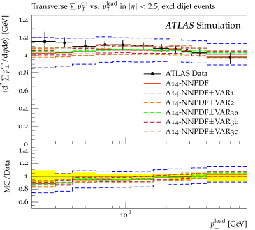
Figure 6: Use of tune uncertainty estimation to predict LHC underlying event activity

The logical conclusion of this is to decide that the ultimate arbiter of how large a parameter change should be is that it produces a model variation comparable to the measured experimental uncertainty on the observables, such that the union of all parameter variations envelopes all or at least most data uncertainties. This approach is the philosophy adopted by several recent Professor-based tunes, such as the A14 series [37], which provide “eigentune” variations to complement the global fit — an example is shown in Figure 6.

The additional detail in eigentune construction is that there are an infinity of ways in which to make model variations “cover” all data, so we prefer a set of variations which are maximally decoupled from one another. This can be achieved by use of a second-order approximation to the $\chi^{2}$ valley around the global optimum: in general this will be an ellipsoid in the parameter space, and the principal basis of this ellipsoid defines $2P$ principal vectors along which to make parameter variations. These vectors are obtained as the eigenbasis of the covariance matrix computed at the global tune point.

If the test statistic were truly distributed according to the $\chi^{2}$ distribution, the required deviation could be calculated analytically from the $\chi^{2}(k,x)$ distribution for degree of freedom $k=N_{\mathrm{bins}}-P$, by making pairs of deviations along the $P$ eigenvectors until the $\chi^{2}$ corresponding to a $p$-value of e.g. $1\sigma$ is found: for a perfect $\chi^{2}$ statistic and a best-fit value of $\chi^{2}_{\mathrm{best}}\sim k$, this should require a $\Delta\chi^{2}$ shift of $\sim\!2k/3$. But in practice we find that such a construction fails the “reasonableness test”: the resulting variations are far too small. Empirically, the typical distribution in global LHC fits has a much larger mean than expected for the number of degrees of freedom, and a narrow spread incompatible with the $\chi^{2}$ distribution’s relation between mean and variance. Instead the strategy of producing empirical model variations which cover the experimental uncertainties has been adopted in tune sets such as A14, requiring a $\Delta\chi^{2}\sim N/2$ to produce experimentally useful systematic variations. Other, less empirical, approaches are still being explored.

It is thought that this deviation from statistical expectation largely stems from the fact that we do not yet have models capable of reproducing all data observables: “the truth” is not contained in the model space. In addition, the data available so far for MPI tuning have not included detailed bin-to-bin correlations from systematic uncertainties, which in principle could be eliminated by a nuisance parameter fit — this futher distorts the goodness-of-fit measure away from the $\chi^{2}$ distribution. Finally, there is the ever-present risk of underestimated experimental uncertainties. There is hence still potential to improve tuning methodology, by construction of more robustly motivated systematic variations and reducing tuning uncertainties by fully correlated likelihood construction across multiple measurements.

In addition to the eigentune method described here, a full assessment of tuning uncertainties should coherently encompass statistical uncertainties in the Professor parameterisation construction (estimated by making many semi-independent parameterisations, from subsets of the available MC runs), and correlations in $\chi^{2}$ construction. Accurate treatment of these effects may eventually permit tune uncertainties to be treated on the same statistical level as those of parton density function fits.

5 Outlook

Tuning has proven to be an important activity in the development of MC models of initial-state QCD at the LHC, both by providing the experiments with unprecedentedly well-honed simulations of collision events (including pile-up), but also by providing a mechanism by which to unambiguously identify when a model’s limitations are fundamental. At the same time, the development of tuning machinery for the LHC has provided ways to quantitatively estimate model and tune uncertainties, and in principle to reduce them — although the statistical foundation still requires development.

Technically, the Professor framework has seen recent advances, originally developed for BSM physics studies but readily applied to QCD MC tuning: the most obvious of these are the inclusion of non-polynomial functional forms such as neural nets, suport vector machines, and methods based on decision trees. Work on using Gaussian processes, along with more refined statistical testing of parameterisation fidelity, offer the possibility of yet more accurate MC parameterisation for use in fitting. In parallel, a serial Markov chain approach to tuning, based on Bayesian parameter optimisation has been developed and appears interesting, if yet unproven on the large-scale problem of initial-state QCD tuning where the MC runs are very computationally expensive [41].

The most painful price paid for the increasing LHC demands of simulation accuracy has been the proliferation of tunes specific to process types: underlying event vs. inclusive minimum-bias, or QCD-singlet vs. coloured hard-processes. Such fragmentation is undesirable because it implies a lack of predictivity in the models: if we cannot trust an MPI+shower model to simultaneously describe minimum-bias and underlying event, how confident can we be about its extrapolation to more rarified regions of phase-space? The resolution of this problem, and the coherent integration of diffractive processes and hence the connection between fiducial and total inelastic scattering cross-sections, must be the main challenges for development and tuning of MC models in the coming years. While technology has helped the development of tunes through the early phase of the LHC, in the end it must be coupled to physics insights to achieve the goal of truly comprehensive description of hadronic initial-state interactions.

References

- [1] P. Skands, S. Carrazza, and J. Rojo, Tuning PYTHIA 8.1: the Monash 2013 Tune, Eur. Phys. J. C74(8), 3024 (2014). 10.1140/epjc/s10052-014-3024-y.
- [2] S. Kama. Automatic Monte-Carlo Tuning for Minimum Bias Events at the LHC. PhD thesis, DESY (2010-03-24). URL https://inspirehep.net/record/1186251/files/CERN-THESIS-2010-259.pdf.
- [3] A. Buckley, H. Hoeth, H. Lacker, H. Schulz, and J. E. von Seggern, Systematic event generator tuning for the LHC, Eur. Phys. J. C65, 331–357 (2010). 10.1140/epjc/s10052-009-1196-7.
- [4] C. Patrignani et al., Review of Particle Physics, Chin. Phys. C40(10), 100001 (2016). 10.1088/1674-1137/40/10/100001.
- [5] P. Abreu et al., Tuning and test of fragmentation models based on identified particles and precision event shape data, Z. Phys. C73, 11–60 (1996). 10.1007/s002880050295.
- [6] R. Barate et al., Studies of quantum chromodynamics with the ALEPH detector, Phys. Rept. 294, 1–165 (1998). 10.1016/S0370-1573(97)00045-8.
- [7] P. Pfeifenschneider et al., QCD analyses and determinations of alpha(s) in e+ e- annihilation at energies between 35-GeV and 189-GeV, Eur. Phys. J. C17, 19–51 (2000). 10.1007/s100520000432.
- [8] B. Abelev et al., Measurement of inelastic, single- and double-diffraction cross sections in proton–proton collisions at the LHC with ALICE, Eur. Phys. J. C73(6), 2456 (2013). 10.1140/epjc/s10052-013-2456-0.
- [9] F. Abe et al., Pseudorapidity distributions of charged particles produced in interactions at GeV and 1800 GeV, Phys. Rev. D41, 2330 (1990). 10.1103/PhysRevD.41.2330. [,119(1989)].
- [10] D. Acosta et al., Soft and hard interactions in collisions at 1800-GeV and 630-GeV, Phys. Rev. D65, 072005 (2002). 10.1103/PhysRevD.65.072005.
- [11] T. Aaltonen et al., Measurement of Particle Production and Inclusive Differential Cross Sections in Collisions at -TeV, Phys. Rev. D79, 112005 (2009). 10.1103/PhysRevD.82.119903, 10.1103/PhysRevD.79.112005. [Erratum: Phys. Rev.D82,119903(2010)].
- [12] G. Aad et al., Charged-particle multiplicities in interactions at GeV measured with the ATLAS detector at the LHC, Phys. Lett. B688, 21–42 (2010). 10.1016/j.physletb.2010.03.064.
- [13] G. Aad et al., Charged-particle multiplicities in pp interactions measured with the ATLAS detector at the LHC, New J. Phys. 13, 053033 (2011). 10.1088/1367-2630/13/5/053033.
- [14] G. Aad et al., Charged-particle distributions in = 13 TeV pp interactions measured with the ATLAS detector at the LHC, Phys. Lett. B758, 67–88 (2016). 10.1016/j.physletb.2016.04.050.
- [15] G. Aad et al., Charged-particle distributions in interactions at 8 TeV measured with the ATLAS detector, Eur. Phys. J. C76(7), 403 (2016). 10.1140/epjc/s10052-016-4203-9.
- [16] M. Aaboud et al., Charged-particle distributions at low transverse momentum in TeV interactions measured with the ATLAS detector at the LHC, Eur. Phys. J. C76(9), 502 (2016). 10.1140/epjc/s10052-016-4335-y.
- [17] V. Khachatryan et al., Charged particle multiplicities in interactions at , 2.36, and 7 TeV, JHEP. 01, 079 (2011). 10.1007/JHEP01(2011)079.
- [18] G. Aad et al., Measurement of the underlying event in jet events from 7 TeV proton-proton collisions with the ATLAS detector, Eur. Phys. J. C74(8), 2965 (2014). 10.1140/epjc/s10052-014-2965-5.
- [19] S. Chatrchyan et al., Measurement of the Underlying Event Activity at the LHC with TeV and Comparison with TeV, JHEP. 09, 109 (2011). 10.1007/JHEP09(2011)109.
- [20] V. Khachatryan et al., Measurement of the underlying event activity using charged-particle jets in proton-proton collisions at sqrt(s) = 2.76 TeV, JHEP. 09, 137 (2015). 10.1007/JHEP09(2015)137.
- [21] T. Aaltonen et al., Studying the Underlying Event in Drell-Yan and High Transverse Momentum Jet Production at the Tevatron, Phys. Rev. D82, 034001 (2010). 10.1103/PhysRevD.82.034001.
- [22] G. Aad et al., Measurement of distributions sensitive to the underlying event in inclusive Z-boson production in collisions at TeV with the ATLAS detector, Eur. Phys. J. C74(12), 3195 (2014). 10.1140/epjc/s10052-014-3195-6.
- [23] D. Acosta et al., The underlying event in hard interactions at the Tevatron collider, Phys. Rev. D70, 072002 (2004). 10.1103/PhysRevD.70.072002.
- [24] A. Buckley, Sensitivities to PDFs in parton shower MC generator reweighting and tuning (2016).
- [25] A. Donnachie and P. V. Landshoff, Small x: Two pomerons!, Phys. Lett. B437, 408–416 (1998). 10.1016/S0370-2693(98)00899-5.
- [26] H. Schulz and P. Z. Skands, Energy Scaling of Minimum-Bias Tunes, Eur. Phys. J. C71, 1644 (2011). 10.1140/epjc/s10052-011-1644-z.
- [27] S. Frixione, P. Nason, and C. Oleari, Matching NLO QCD computations with Parton Shower simulations: the POWHEG method, JHEP. 11, 070 (2007). 10.1088/1126-6708/2007/11/070.
- [28] M. Althoff et al., Determination of in First and Second Order QCD From Annihilation Into Hadrons, Z. Phys. C26, 157 (1984).
- [29] W. Braunschweig et al., Jet Fragmentation and QCD Models in Annihilation at .m. Energies Between 12-GeV and 41.5-GeV, Z. Phys. C41, 359–373 (1988). 10.1007/BF01585620.
- [30] D. Buskulic et al., Properties of hadronic Z decays and test of QCD generators, Z. Phys. C55, 209–234 (1992). 10.1007/BF01482583.
- [31] K. Hamacher and M. Weierstall, The Next round of hadronic generator tuning heavily based on identified particle data (1995).
- [32] F. Feroz, M. P. Hobson, E. Cameron, and A. N. Pettitt, Importance Nested Sampling and the MultiNest Algorithm (2013).
- [33] R. Field. CDF Run II Monte-Carlo tunes. In TeV4LHC 2006 Workshop 4th meeting Batavia, Illinois, October 20-22, 2006 (2006).
- [34] T. Affolder et al., Charged jet evolution and the underlying event in collisions at 1.8 TeV, Phys. Rev. D65, 092002 (2002). 10.1103/PhysRevD.65.092002.
- [35] T. Affolder et al., The transverse momentum and total cross section of pairs in the boson region from collisions at TeV, Phys. Rev. Lett. 84, 845–850 (2000). 10.1103/PhysRevLett.84.845.
- [36] V. M. Abazov et al., Measurement of dijet azimuthal decorrelations at central rapidities in collisions at TeV, Phys. Rev. Lett. 94, 221801 (2005). 10.1103/PhysRevLett.94.221801.
- [37] ATLAS Run 1 Pythia8 tunes. Technical Report ATL-PHYS-PUB-2014-021, CERN, Geneva (Nov, 2014). URL https://cds.cern.ch/record/1966419.
- [38] V. Khachatryan et al., Event generator tunes obtained from underlying event and multiparton scattering measurements, Eur. Phys. J. C76(3), 155 (2016). 10.1140/epjc/s10052-016-3988-x.
- [39] Example ATLAS tunes of Pythia8, Pythia6 and Powheg to an observable sensitive to boson transverse momentum. Technical Report ATL-PHYS-PUB-2013-017, CERN, Geneva (Nov, 2013). URL https://cds.cern.ch/record/1629317.
- [40] A study of the sensitivity to the Pythia8 parton shower parameters of production measurements in collisions at TeV with the ATLAS experiment at the LHC. Technical Report ATL-PHYS-PUB-2015-007, CERN, Geneva (Mar, 2015). URL https://cds.cern.ch/record/2004362.
- [41] P. Ilten, M. Williams, and Y. Yang, Event generator tuning using Bayesian optimization, JINST. 12(04), P04028 (2017). 10.1088/1748-0221/12/04/P04028.