LAPTH-026/18 Stationary double black hole
without naked ring singularity

Abstract

Recently double black hole vacuum and electrovacuum metrics attracted attention as exact solutions suitable for visualization of ultra-compact objects beyond the Kerr paradigm. However, many of the proposed systems are plagued with ring curvature singularities. Here we present a new simple solution of this type which is asymptotically Kerr, has zero electric and magnetic charges, but is endowed with magnetic dipole moment and electric quadrupole moment. It is manifestly free of ring singularities, and contains only a mild string-like singularity on the axis corresponding to a distributional energy-momentum tensor. Its main constituents are two extreme co-rotating black holes carrying equal electric and opposite magnetic and NUT charges.

I Introduction

Binary black holes became an especially hot topic after the discovery of the first gravitational wave signal from merging black holes Barack:2018yly . A particular interest lies in determining their observational features other than emission of strong gravitational waves. Such features include gravitational lensing and shadows which presumably can be observed in experiments such as the Event Horizon Telescope and future space projects. For these experiments to have sense, one needs to model plausible alternatives to the Kerr paradigm Yagi . Most proposed scenarios use phenomenologically constructed metrics such as deformed Kerr, or “bumpy” black holes, not necessarily satisfying the Einstein equations, or exact solutions for black holes with hair, and black holes in modified gravity to study lensing/shadow pictures Cunha:2018acu .

Some popular lensing/shadow models use the double Kerr solution of Kramer and Neugebauer Kramer1980 ; Costa:2010zzg describing two rotating Kerr black holes sitting on the same axis, as well as more general vacuum and electrovacuum solutions for double black holes (DBH) Cunha:2018gql ; Cunha:2018cof . One should be warned, however, that typically DBH solutions contain strong curvature singularities in the physical region, which are often overlooked or ignored Johannsen:2013rqa . Solutions with strong naked curvature singularities should certainly be rejected as unphysical. At the same time, in view of uniqueness theorems for Kerr black hole, to go beyond the Kerr paradigm one should tolerate violation of some standard assumptions, preferably those which were not rigorously proven. In our opinion, mild violations of cosmic censorship, rejecting strong naked curvature singularities, while admitting distributional ones, such as conical singularities associated with infinitely thin cosmic strings, deserve to be explored more closely. From the theory of cosmic strings. it is known that such singularities can be removed by the introduction of suitable additional matter, so their presence in DBHs can be regarded just as evidence for extra matter, maybe exotic. In view of unsolved dark matter and dark energy problems, such metrics should not be rejected.

With this motivation, we present here a detailed discussion of a new DBH solution of Einstein-Maxwell equations (a short presentation was given in Clement:2017kas ) devoid of strong curvature singularities but containing a string singularity between the constituent black holes. This solution was first constructed, not by the soliton technique which is now the main tool in the domain of exact solutions, but by applying an original approach of one of the authors GC98 which opens a way to generate rotating electrovacuum solutions generically not accessible by soliton dressing.

An early solution, the magnetic dipole of Bonnor (1966) Bonnor:1966 , was later reinterpreted as a dihole: a static system of two extremal black holes with opposite magnetic charges Emparan:1999au ; Emparan:2001bb . Another early family of stationary vacuum solutions was that of “deformed” Kerr metrics given by Tomimatsu and Sato Tomimatsu:1972zz (TS) with the integer deformation parameter $\delta$, such that the Kerr metric is reproduced for $\delta=1$. Its $\delta=2$ member was later interpreted as a DBH. In fact, the static version of the Tomimatsu-Sato solution with $\delta=2$ (TS2) was known since the papers by Bach and Weyl (1922) BW , Darmois (1927) darmois , Zipoy (1966) Zipoy1966 and Voorhees (1971) Voorhees:1971wh (ZV). These solutions, expressed in prolate spheroidal coordinates ($x,y$), exhibit directional singularities at $x=1,y=\pm 1$ gibbons73 . The two-surface nature of the “points” $x=1,y=\pm 1$ of the TS2 solution, hinted at in Ernst ; Economou , was then explicitly demonstrated by Papadopoulos et al. in 1981 Papadopoulos:1981wr showing that these are black hole horizons. Still, misinterpretation persisted in some papers (see e.g. Manko:1999xg ), until it was unambiguosly proven by Kodama and Hikida Kodama:2003ch that both ZV2 and TS2 are DBH solutions indeed, though singular (for modern analysis and applications also see Gegenberg:2010np ). The Tomimatsu-Sato family, apart from the “deformation” parameter $\delta$, have only two physical parameters which can be chosen as the total mass and angular momentum, as for the Kerr metric. The Kerr uniqueness is circumvented in this case because the TS2 metric contains a naked ring singularity in the domain of outer communications Tomimatsu:1972zz . Our solution can be interpreted as a new rotating electrovacuum extension of the ZV2 solution different from TS2 as well as from previously known electrovacuum extensions of TS2 Ernst1 ; Manko:1999xg , which are also plagued with strong naked singularities.

A new hunt for double-center solutions started with Kramer and Neugebauer Kramer1980 , who applied Bäcklund transformations Hoenselaers:1985qk to construct two-black hole solutions with the individual masses, angular momenta, and NUT charges of the constituents, together with the distance between them, as free parameters. Soon after it was realized that the inverse scattering method (ISM) of Belinski and Zakharov Belinsky:1979mh ; Belinski:2001ph is a more universal and convenient tool to produce DBH solutions via soliton dressing of black-hole backgrounds (for a review and further references see an accessible introduction by Herdeiro et al. Herdeiro:2008kq , an extensive book by Griffiths and Podolsky GP , and a more recent paper by Alekseev Alekseev:2017zuh ). It is worth noting that the method used in the current paper, though it generates only a one-parameter family of new solutions, is applicable in the case of generic non-analytic metrics where the ISM does not work. In the case of applicability of ISM both methods lead to identical results.

One of the main problems in the DBH theory was the search for equilibrium configurations of two vacuum or charged black holes. It has been known for some time that equilibrium of two centers generically carrying masses and electric (magnetic) charges is possible only in the case when masses and charges satisfy the so-called no-force conditions Breitenlohner:1987dg . The corresponding solutions are characterized by conformally flat three-metrics, so that consequently multi-center solutions may exist for any positions of the centers (Majumdar-Papapetrou multi-black hole solution). But, two-center solutions can also exist for a certain separation between the centers, with a quite different relationship between the parameters Bonnor:1993 ; Perry , though these have naked singularities.

An intriguing question was whether the gravitational spin-spin interaction, which is repulsive for parallel spins, can overcome gravitational attraction. The extremal co-rotating Kerr black holes seem to be most favored for this. General conditions for force balance were formulated by Tomimatsu and collaborators Tomimatsu:1981bc ; Kihara:1981mx ; Tomimatsu:1983qc , but the first found rotating configurations obeying these conditions were shown to contain strong naked singularities. A thorough investigation of double-Kerr solutions by Dietz and Hoenselaers Dietz1985 led to the conclusion that the balance is not possible for two black holes with regular horizons, unless hyperextreme objects (which are not black holes, but naked singularities) are involved. Later, several non-existence theorems for stationary balanced vacuum two-black hole systems (including extremal black holes) were formulated by Neugebauer and Hennig Neugebauer:2009su ; Hennig:2011fp ; Neugebauer:2011qb , see also Chrusciel:2011iv . The conclusion following from this analysis is that to balance two asymptotically flat black holes one needs conical singularities (a cosmic string) on the axis between the centers. Similar conclusions were derived in the electrovacuum case Alekseev:2012au .

An additional restriction comes from the requirement that the string be non-rotating, since otherwise it will be surrounded by a region where $g_{\varphi\varphi}$ changes sign, implying the existence of closed timelike curves (CTC). For two rotating black holes this causes additional restrictions on the parameters, excluding in particular the possibility of NUT charges of the constituents (“axis conditions”). Here we do not introduce these restrictions, and allow for the possibility of rotating cosmic strings. In so doing, we enlarge the family of metrics with a distributional Ricci tensor, which indicates that new forms of matter should be involved. On the other hand, we exclude ring curvature singularities in the physical region, since these can in no case be smoothed out by additional matter sources.

II Constructing the solution

II.1 The seed

Our new solution was constructed using the original generating technique of GC98 , with a seed belonging to the Weyl stationary axisymmetric class, the static ZV2 vacuum solution. In the standard Weyl-Papapetrou parametrization

$$ds^{2}=-F(dt-\omega d\varphi)^{2}+F^{-1}[e^{2k}(d\rho^{2}+dz^{2})+\rho^{2}d\varphi^{2}],$$ (2.1)

the ZV2 solution Zipoy1966 ; Voorhees:1971wh , first given by Darmois darmois , is characterized by

$$F=\left(\displaystyle\frac{x-1}{x+1}\right)^{2},\quad e^{2k}=\left(\displaystyle\frac{x^{2}-1}{x^{2}-y^{2}}\right)^{4},\quad\omega=0,$$ (2.2)

where the prolate spheroidal coordinates $(x,y)$ are related to the Weyl coordinates by

$$\rho=\kappa(x^{2}-1)^{1/2}(1-y^{2})^{1/2},\quad z=\kappa xy$$ (2.3)

(the positive constant $\kappa$ setting the length scale).

This solution is asymptotically (as $x\to\infty$) flat and has the Schwarzschild mass $M=2\kappa$, which can be easily seen by using the asymptotic identification

$$x\approx r/\kappa-1+{\rm O}(1/r),\quad y=\cos\theta.$$ (2.4)

To reveal the singularities, one computes the Kretschmann scalar $K=R_{\mu\nu\lambda\tau}R^{\mu\nu\lambda\tau}$, obtaining

$$K=\frac{192(x^{2}-y^{2})^{5}}{\kappa^{2}(x^{2}-1)^{6}(x+1)^{8}}\left[x^{4}-4x^{3}+(7-4y^{2})x^{2}+(10y^{2}-6)x-7y^{2}+3\right].$$ (2.5)

The coordinate region $x\geq 1,\,|y|\leq 1$ thus presents an asymptotically flat space-time with a curvature singularity at $x=1$ and $|y|<1$, which corresponds to an open set in the Weyl coordinates $\rho=0,\,-\kappa<z<\kappa$ (the singular rod).

The boundary points of the rod $z=\pm\kappa$ are directional singularities. If one approaches $z=\kappa,\,\rho=0$ sending $x\to 1,y\to 1$ and keeping the ratio $X^{2}=(1-y^{2})/(x^{2}-1)$ fixed (with $Y=y/x\to 1$ ), one finds that the Kretschmann scalar depends on $X$,

$$K_{H}=\lim_{Y\to\pm 1}K=\frac{3(X^{2}+1)^{6}}{4\kappa^{4}},$$ (2.6)

and diverges as $X\to\infty$. The same value of $K$ will be obtained approaching $z=-\kappa$ with fixed $X$, in which case $Y\to-1$. Following Kodama:2003ch and using $X,\,Y$ as new coordinates,

$$X=\sqrt{\frac{1-y^{2}}{x^{2}-1}},\;\;Y=\frac{y}{x},\quad x=\sqrt{\frac{X^{2}+1}{X^{2}+Y^{2}}},\;\;y=Y\,\sqrt{\frac{X^{2}+1}{X^{2}+Y^{2}}},$$ (2.7)

one can see that the infinite value $X=\infty$ corresponds to the singular open set $\rho=0,\,-\kappa<z<\kappa$, while the limiting “points” $\rho=0,\,z=\pm\kappa$ are actually two-surfaces $Y=\pm 1$. Using the relations

$$x^{2}-1=\frac{1-Y^{2}}{X^{2}+Y^{2}},\quad 1-y^{2}=\frac{X^{2}(1-Y^{2})}{X^{2}+Y^{2}},\quad x^{2}-y^{2}=\frac{(X^{2}+1)(1-Y^{2})}{X^{2}+Y^{2}},$$

$$\rho=\frac{\kappa X(1-Y^{2})}{X^{2}+Y^{2}},\quad z=\frac{\kappa Y(X^{2}+1)}{X^{2}+Y^{2}},$$ (2.8)

$$d\rho^{2}+dz^{2}=\kappa^{2}(x^{2}-y^{2})\left(\frac{dx^{2}}{x^{2}-1}+\frac{dy^{2}}{1-y^{2}}\right)=\kappa^{2}(x^{2}-y^{2})^{2}\left[\frac{dX^{2}}{(X^{2}+1)^{2}}+\frac{dY^{2}}{(1-Y^{2})^{2}}\right],$$

one can rewrite the metric in the vicinity of $Y=\pm 1$ as

$$ds_{\pm}^{2}=\frac{1}{(X^{2}+1)^{2}}\left[-\frac{(1\mp Y)^{2}}{4}\,dt^{2}+\frac{4\kappa^{2}}{(1\mp Y)^{2}}\,dY^{2}\right]+16\kappa^{2}\left[\frac{dX^{2}}{(X^{2}+1)^{4}}+X^{2}d\varphi^{2}\right]\,.$$ (2.9)

Apparently, these metrics describe two extremal black holes with degenerate horizons $H_{\pm}$ at $Y=\pm 1$, and finite horizon area Kodama:2003ch

$${\cal A}_{H}=32\pi\kappa^{2}\int_{0}^{\infty}\frac{XdX}{(X^{2}+1)^{2}}=16\pi\kappa^{2}.$$ (2.10)

Kodama and Hikida Kodama:2003ch have constructed an analytic continuation through the horizons to other Lorentzian sectors $|y|>1,|x|<1$. However these horizons are not regular, but share the ring-like curvature singularity $X\to\infty$ as common boundary. They have also shown that the Komar mass of this singularity is equal to the total mass $M=2\kappa$ (which is unusual for naked singularities typically corresponding to negative mass), so that the black holes themselves are massless.

The ZV2 metric has two Killing symmetries ($\partial_{t}$ and $\partial_{\varphi}$) and no second-order Killing tensors, so the geodesic equations and the wave equations are not separable. While equatorial motion can be explored in a closed form, the non-equatorial orbits can be studied only numerically and generically exhibit chaotic features. Recently this metric attracted attention as an alternative to standard black holes and the corresponding shadows were constructed Cunha:2018acu .

Rotating vacuum generalizations were constructed for integer $\delta$ by Tomimatsu and Sato Tomimatsu:1972zz , who showed that the $\delta=2$ rotating solution (TS2) has a naked ring singularity. As discussed by Gibbons and Russel-Clark gibbons73 , it also has a causal boundary ($g_{\varphi\varphi}=0$), and a non-curvature Misner-string singularity at $x=1$. The subsequent analysis of Kodama and Hikida Kodama:2003ch revealed that the segment $x=1$ is generically a line of conical singularities (cosmic string) connecting two degenerate, topologically spherical horizons at $x=\pm y=1$. Thus, the rotating TS2 solution is more regular than the ZV2 solution.

II.2 Clément transformation

The four-dimensional stationary Einstein-Maxwell equations are invariant under an $SU(2,1)$ group of transformations Kinnersley:1978pz ; Kinnersley:1978 . These transformations map asymptotically flat monopole solutions into monopole solutions, and so cannot be used to transform an axisymmetric static monopole solution into a rotating monopole–dipole solution. It was shown in GC98 that this goal could be achieved by combining $SU(2,1)$ transformations changing the asymptotic behavior with linear coordinate transformations in the plane of the two Killing vectors, leading to a special finite Geroch transformation.

More precisely, the rotation–generating transformation is the product

$$\Sigma=\Pi^{-1}\,{\cal R}(\Omega)\,\Pi$$ (2.11)

of three successive transformations, two “vertical” transformations $\Pi\,,\Pi^{-1}\in$ SU(2,1) acting on the space of the complex Ernst potentials ${\cal E}$ and $\psi$, and a “horizontal” global coordinate transformation ${\cal}R(\Omega)$ acting on the Killing 2–plane. The transformation $\Pi:\;({\cal E},\psi)\leftrightarrow(\hat{\cal E},\hat{\psi})$ with

$$\hat{\cal E}=\frac{-1+{\cal E}\pm 2\psi}{1-{\cal E}+\pm 2\psi}\,,\quad\hat{\psi}=\mp\frac{1+{\cal E}}{1-{\cal E}\pm 2\psi}\,.$$ (2.12)

leads from an asymptotically flat monopole seed solution to one which asymptotes to $AdS_{2}\times S^{2}$, i.e, is asymptotically Bertotti-Robinson (BR)-like. The global coordinate transformation ${\cal R}(\Omega,\gamma(\Omega))$ is the product of the transformation to a uniformly rotating frame and of a time dilation,

$$d\varphi=d\varphi^{\prime}+\Omega\gamma\,dt^{\prime}\,,\qquad dt=\gamma\,dt^{\prime}\,.$$ (2.13)

This does not modify the leading asymptotic behavior of asymptotically BR–like metrics, so that the last transformation $\Pi^{-1}$ in (2.11) then leads to a new asymptotically flat solution with a dipole gravimagnetic moment proportional to $\Omega$, ie. a rotating solution. In the case of a vacuum seed solution, the parameter $\gamma(\Omega)$ can be chosen so that this new solution has no monopole electromagnetic charges, but it will generically (except in the case of the Schwarzschild seed, which leads to the neutral Kerr solution) have a dipole magnetic moment and a quadrupole electric moment.

II.3 New solution

The new rotating solution generated from the ZV2 solution by the transformation $\Sigma$ can be given in terms of the Kinnersley potentials:

$$U = p\displaystyle\frac{x^{2}+1}{2x}+iqy,\qquad V=\varepsilon(W-1),$$

$$W = 1+\displaystyle\frac{q^{2}}{2}\displaystyle\frac{1-y^{2}}{x^{2}-1}-i\displaystyle\frac{pq}{2}\displaystyle\frac{y}{x},\qquad(\varepsilon^{2}=1),$$ (2.14)

related to the complex Ernst potentials by

$${\cal E}=(U-W)/(U+W),\qquad\psi=V/(U+W).$$ (2.15)

The real parameters $p$ and $q$ are related by $p=\sqrt{1-q^{2}}$ so that, just as the TS2 solution, this family of solutions depends on the single dimensionless rotation parameter $q$ (proportional to $\Omega$). The potentials of the ZV2 solution are recovered for $q=0$.

The form (II.3) of the solution is only implicit. Dualization of the imaginary part of the scalar Ernst potentials to vector potentials leads to the explicit metric

$$ds^{2} = -\frac{f}{\Sigma}\left(dt-\frac{\kappa\Pi}{f}\,d\varphi\right)^{2}+\kappa^{2}\Sigma\left[e^{2\nu}\left(\frac{dx^{2}}{x^{2}-1}+\frac{dy^{2}}{1-y^{2}}\right)\right.$$ (2.16)

$$\left.\quad+f^{-1}(x^{2}-1)(1-y^{2})d\varphi^{2}\right],$$

where $\varphi$ is periodic with period $2\pi$ as before, and the Weyl metric functions are split as follows:

$$F=\frac{f}{\Sigma},\quad\omega=\frac{\kappa\Pi}{f},\quad e^{2k}=\frac{fe^{2\nu}}{x^{2}-y^{2}},$$ (2.17)

with

$$f = \frac{p^{2}(x^{2}-1)^{2}}{4x^{2}}-\frac{q^{2}x^{2}(1-y^{2})}{x^{2}-1},$$ (2.18)

$$\Sigma = \left[\frac{px^{2}+2x+p}{2x}+\frac{q^{2}(1-y^{2})}{2(x^{2}-1)}\right]^{2}+q^{2}\left(1-\frac{p}{2x}\right)^{2}y^{2},$$ (2.19)

$$e^{2\nu} = \frac{4x^{2}(x^{2}-1)^{2}}{p^{2}(x^{2}-y^{2})^{3}},$$ (2.20)

Note that $\Sigma$ is positive definite. The rotation function $\omega$ is proportional to the second order polynomial in $(1-y^{2})$:

$$\Pi=\Pi_{1}(x)(1-y^{2})+\Pi_{2}(x)(1-y^{2})^{2},$$ (2.21)

with $x$-dependent coefficients

$$\Pi_{1} = -\frac{q}{2p}\left\{\frac{(px+2)[4x^{2}+p^{2}(x^{2}-1)]}{x^{2}}+\frac{4p(1+p^{2})x+8+p^{2}-p^{4}}{x^{2}-1}\right\},$$ (2.22)

$$\Pi_{2} = -\frac{q^{3}}{2}\left[\frac{p}{4x^{2}}+\frac{2x-p}{x^{2}-1}\right].$$ (2.23)

This is a stationary axisymmetric solution of the Einstein-Maxwell equations, whose electromagnetic part is given by the four-potential $A=A_{0}(x,y)dt+A_{\varphi}(x,y)d\varphi$, with

$$A_{0}=\frac{\varepsilon\overline{v}}{\Sigma},\quad A_{\varphi}=\frac{\varepsilon\kappa\Theta}{\Sigma},$$ (2.24)

where

$$\overline{v}=\frac{q^{2}}{4}\left\{-\frac{p(2x-p)}{x^{2}}+\left[\frac{p(2x-p)}{x^{2}}+\frac{px^{2}+2x+p}{x(x^{2}-1)}\right](1-y^{2})+\frac{q^{2}(1-y^{2})^{2}}{(x^{2}-1)^{2}}\right\},$$ (2.25)

$\varepsilon=\pm 1$, and $\Theta$ is the third order polynomial in $1-y^{2}$:

$$\Theta=\Theta_{1}(x)(1-y^{2})+\Theta_{2}(x)(1-y^{2})^{2}+\Theta_{3}(x)(1-y^{2})^{3},$$ (2.26)

with $x$-dependent coefficients

$$\Theta_{1}= -\frac{q}{4p}\left\{\frac{p\left[p^{2}x^{3}+5px^{2}-(8-4p^{2}+p^{4})x+2p-3p^{3}\right]}{x^{2}}+\frac{(16-p^{2}+p^{4})px+8+7p^{2}+p^{4}}{x^{2}-1}\right\},$$ (2.27)

$$\Theta_{2}= -\frac{q^{3}}{8p}\left[\frac{p(4x^{3}-3px^{2}+2p^{2}x+5p)}{x^{2}(x^{2}-1)}+\frac{2(4x+3p+p^{3})}{x(x^{2}-1)^{2}}\right],$$ (2.28)

$$\Theta_{3}= -\frac{q^{5}}{8x(x^{2}-1)^{2}}.$$ (2.29)

This solution is different from the TS2 vacuum solution, but turns out to coincide with a subclass of the four-parameter family of solutions of the Einstein-Maxwell equations constructed by Manko et al. in manko00 , corresponding to the two constraints on their parameters (here indexed with $M$):

$$\delta_{M}=0\quad(\mu_{M}=-m_{M}b_{M},\;d_{M}=k_{M}^{2}),\quad(a_{M}-b_{M})d_{M}=m_{M}^{2}b_{M}.$$ (2.30)

The non-vanishing Manko et al. parameters are related to ours by

$$k_{M}=\kappa,\quad m_{M}=\frac{2\kappa}{p},\quad b_{M}=-\frac{\kappa pq}{2},\quad a_{M}=-\frac{2\kappa q}{p}(1+p^{2}/4),$$ (2.31)

and $m_{M}b_{M}=-\kappa^{2}q$, $a_{M}-b_{M}=-2\kappa q/p$. The correspondence between their metric functions (23) and ours is

$$\frac{f}{E_{M}}=\frac{\Sigma}{D_{M}}=-\kappa\frac{\Pi_{1}+(1-y^{2})\Pi_{2}}{F_{M}}=\frac{p^{2}}{64\kappa^{8}x^{2}(x^{2}-1)^{2}}.$$ (2.32)

III Physical properties

III.1 Asymptotics

The metric (2.16) is asymptotically (for $x\to\infty$) Minkowskian, which can be seen by introducing spherical coordinates (2.4):

$$F \sim 1-\frac{4\kappa}{pr}+O\left(\frac{1}{r^{2}}\right),$$ (3.1)

$$\omega \sim-\frac{2q\kappa^{2}(p^{2}+4)\sin^{2}\theta}{p^{2}r}+O\left(\frac{1}{r^{2}}\right),$$ (3.2)

$$g_{rr} \sim 1+\frac{4\kappa}{pr}+O\left(\frac{1}{r^{2}}\right),$$ (3.3)

$$g_{\theta\theta} \sim r^{2},\quad g_{\varphi\varphi}\sim r^{2}\sin^{2}\theta.$$ (3.4)

The associated mass $M$ and angular momentum $J$ are

$$M=\frac{2\kappa}{p},\quad J=\frac{\kappa^{2}q(4+p^{2})}{p^{2}}.$$ (3.5)

The electromagnetic potential exhibits the following asymptotic behavior:

$$A_{t} \sim\frac{\varepsilon\kappa^{3}q^{2}(1-3\cos^{3}\theta)}{pr^{2}}+O\left(\frac{1}{r^{3}}\right),$$ (3.6)

$$A_{\varphi} \sim-\frac{\varepsilon\kappa^{2}q\sin^{2}\theta}{r}+O\left(\frac{1}{r^{2}}\right).$$ (3.7)

It follows that the total electric and magnetic charges are zero, while there are a magnetic dipole moment $\mu$, and a quadrupole electric moment $Q_{2}$:

$$\mu=\varepsilon\kappa^{2}q,\qquad Q_{2}=-\varepsilon\kappa^{3}q^{2}/p.$$ (3.8)

The ratio $|\mu/J|$ is bounded above by $1/5$, in agreement with the Barrow-Gibbons bound BG $|\mu/J|\leq 1$, while the ratio $|J|/M^{2}$ satisfies the Kerr-like bound

$$|J|/M^{2}=|q|(1+p^{2}/4)\leq 1.$$ (3.9)

The upper bound in (3.9) is attained in the limit $p\to 0$ with $M$ fixed, meaning also $\kappa=pM/2\to 0$. Accordingly one must first, as in the case of the Kerr or Kerr-Newman solutions, rescale the radial coordinate $x$ by

$$x=2\frac{\overline{x}}{p}$$ (3.10)

before taking the limit $p\to 0$, which for fixed $\overline{x}$ sends $x$ to infinity. It follows that the Kinnersley potentials (II.3) go over to

$$U_{\rm lim}=\overline{x}\pm iy,\quad V_{\rm lim}=0,\quad W_{\rm lim}=1,$$ (3.11)

which are those of the extreme Kerr metric. So the rescaled solution interpolates between two limiting vacuum solutions, ZV2 for $q\to 0$ and extreme Kerr for $q\to 1$.

We will show later that, like ZV2, our solution, initially defined in the domain $x\in]1,\infty),y\in[-1,1]$, can be extended through the horizons at $x=|y|=1$ beyond this region. But let us first explore the solution with decreasing $x$ step by step, starting from the region of large $x$ and $y\in[-1,1]$ where $f>0$, $g_{\varphi\varphi}>0$.

III.2 Absence of ring singularity

The first obvious singularities appearing in rotating solutions generated by the method proposed in GC98 are Kerr-like ring singularities corresponding to zeroes of $\Sigma(x,y)$ ($\Sigma$ is the sum of two squares, so $\Sigma(x,y)=0$ actually corresponds to two equations). To the difference of the TS2 vacuum solution, the present solution is free from a naked ring singularity, as it is clear from (2.19) that $\Sigma$ admits the lower bound

$$\Sigma(x,y)>(p+1)^{2}$$ (3.12)

in the region of outer communication $x>1$, $|y|\leq 1$.

III.3 Ergosphere

The solution has two Killing vectors $k=\partial_{t}$ and $m=\partial_{\varphi}$. As $x$ decreases, $k$ eventually becomes null on the ergosurface $f(x,y)=0$,

$$1-y^{2}=\sin^{2}\theta=\frac{p^{2}(x^{2}-1)^{3}}{4q^{2}x^{4}},$$ (3.13)

marking the boundary of the ergosphere where $k$ is spacelike, $g_{tt}>0$. On this ergosurface,

$$g_{\varphi\varphi}\equiv F^{-1}\rho^{2}-F\omega^{2}=\kappa^{2}\left[\frac{\Sigma}{f}(x^{2}-1)(1-y^{2})-\frac{\Pi^{2}}{\Sigma f}\right]$$ (3.14)

is the difference between two terms which both diverge as $f\to 0$. We show in Appendix A that these two poles cancel exactly so that $g_{\varphi\varphi}$ is, as in the case of the Kerr metric, finite and positive on the ergosurface.

As usual, inside the ergosphere the frame dragging effect is manifest, forcing any neutral particle to rotate with an angular velocity $\Omega$ in order that its world-line $x^{\mu}(\tau)$ be time-like, i.e. $g_{\mu\nu}{\dot{x}^{\mu}}{\dot{x}^{\nu}}<0$. This angular velocity must be within the bounds

$$\Omega_{-}<\Omega<\Omega_{+},\qquad\Omega_{\pm}=\frac{-g_{t\varphi}\pm\sqrt{g_{t\varphi}^{2}-g_{tt}g_{\varphi\varphi}}}{g_{\varphi\varphi}}=\frac{-F\omega\pm\rho}{g_{\varphi\varphi}}.$$ (3.15)

In the case of the Kerr metric, the bounding velocities $\Omega_{\pm}$ approach each other with decreasing $x$ till the horizon $\rho=0$, where $\Omega_{-}=\Omega_{+}$ is the angular velocity of rotation of the horizon. In our case the situation appears to be different. When $x$ decreases towards $1$ with $y$ fixed ($|y|<1$), the various metric functions will behave as $f={\rm O}(\xi^{-2})$ ($f$ remaining negative), $\Sigma={\rm O}(\xi^{-4})$, $\Pi={\rm O}(\xi^{-2})$, with $\xi^{2}\equiv x^{2}-1$, so that from (3.14) $g_{\varphi\varphi}$ will be dominated by the constant negative first term. Therefore there is between the ergosphere and the singularity $x=1$ a surface $g_{\varphi\varphi}(x,y)=0$ bounding the chronosphere where $g_{\varphi\varphi}$ stays negative (see below). But, as in the case of the seed ZV2 one can also approach the singularity $x=1$ along a curve $(1-y^{2})/(x^{2}-1)=X^{2}$ constant. Then $f$, $\Sigma$ and $\Pi$ will go to constant values ($f$ remaining again negative), so that now $g_{\varphi\varphi}$ will be dominated by the constant second term in (3.14) and go to finite positive values, depending on the direction $X$, near the coordinate singularities $x=1$, $y=\pm 1$ which, as in the case of ZV2, are actually two disjoint components of the degenerate horizon.

III.4 Horizon

Passing to the coordinates $X,\,Y$ via (2.7), (II.1) one can see that $Y=\pm 1$ are degenerate (second order) horizons with $X$ being related to some angular coordinates on them. Remarkably, while in the seed ZV2 metric the horizons were not topological spheres, in the new solution they are, so the transformation “improved” the horizon geometry. This indicates that the limits $q\to 0$ (ZV2 limit of the solution) and $|Y|\to 1$ (near-horizon) do not commute. This can be seen by writing the function $f$ in $(X,Y)$ coordinates as:

$$f=\frac{1}{(X^{2}+1)(X^{2}+Y^{2})}\left[\frac{p^{2}}{4}(1-Y^{2})^{2}-q^{2}X^{2}(X^{2}+1)^{2}\right]\,.$$ (3.16)

If we set first $q=0$ ($p=1$), $f$ develop a double zero $Y=\pm 1$ corresponding to the double horizon of the ZV2 degenerate static metric as in (2.9) while, for non-zero $q$, $f$ goes to a non-zero limit $f_{H}$ for $|Y|\to 1$. We have

$$f_{H}(X) = -q^{2}X^{2},\quad\Pi_{H}(X)=-q\lambda(p)X^{2},$$

$$\Sigma_{H}(X) = \frac{p\lambda(p)}{2}+q^{2}(1+p)X^{2}+\frac{q^{4}}{4}X^{4},\quad e^{2\nu}=\frac{4}{p^{2}(1-Y^{2})(X^{2}+1)^{2}}\,,$$ (3.17)

with

$$\lambda(p)=\frac{(1+p)(8-4p+5p^{2}-p^{3})}{2p}\geq 8$$ (3.18)

(the lower bound being attained in the limit $q\to 0$).

Inserting these behaviors in (3.14), we find that $g_{\varphi\varphi}$ goes over to a positive function of $X$

$$g_{\varphi\varphi}|_{H}(X)=\frac{\kappa^{2}[\lambda(p)]^{2}X^{2}}{\Sigma_{H}(X)}$$ (3.19)

including the case $q=0$ (the static ZV2 metric), in agreement with the result obtained in Kodama:2003ch . The Weyl coordinate $\rho=\kappa X(1-Y^{2})/(X^{2}+Y^{2})$ goes to zero for $Y\to\pm 1$ so that, from (3.15), the Killing vector $K=\partial_{t}-\Omega_{H}\partial_{\varphi}$ becomes null for $Y=\pm 1$, where the angular velocity of the two-component horizon is

$$\Omega_{H}=\lim_{|Y|\to 1}\Omega_{\pm}=\left.-\frac{\kappa\Pi}{\Sigma g_{\varphi\varphi}}\right|_{H}=\left.\frac{f}{\kappa\Pi}\right|_{H}=\frac{q}{\kappa\lambda(p)}.$$ (3.20)

In the horizon co-rotating frame $(\hat{t},X,Y,\hat{\varphi})$ defined by $\hat{t}=t$, $\hat{\varphi}=\varphi-\Omega_{H}t$, the two-dimensional sections of the two horizon components $Y=\pm 1$ have the same metric:

$$ds_{H}^{2}=\frac{4\kappa^{2}\Sigma(X)dX^{2}}{p^{2}(X^{2}+1)^{4}}+\frac{\kappa^{2}\lambda^{2}(p)X^{2}d\hat{\varphi}^{2}}{\Sigma(X)},$$ (3.21)

Introducing a new angular coordinate $\eta$ by

$$X=\tan(\eta/2)\quad(0\leq\eta\leq\pi),$$ (3.22)

(3.21) can be rewritten as

$$ds_{H}^{2}=\frac{\kappa^{2}\lambda(p)}{2pl(\eta)}\left[d\eta^{2}+l^{2}(\eta)\sin^{2}\eta d\hat{\varphi}^{2}\right],$$ (3.23)

where

$$l(\eta)=\frac{p\lambda(p)}{2}\frac{(X^{2}+1)^{2}}{\Sigma(X)}$$ (3.24)

is everywhere positive and finite. It follows that each horizon is homeomorphic to $S^{2}$.

From (3.21) or (3.23) we obtain the horizon area

$${\cal A}_{H}=4\pi\kappa^{2}\frac{\lambda(p)}{2p}.$$ (3.25)

The corresponding areal radius is of the order of the total mass $M$. More precisely, for small $q$, ${\cal A}_{H}\simeq 16\pi\kappa^{2}$, which leads to a total horizon area $2{\cal A}_{H}(p=1)=32\pi\kappa^{2}=8\pi M^{2}$, as in the static ZV2 case. This is one-half of the horizon area for a Schwarzschild black hole of the same asymptotic mass. The horizon area decreases monotonically with increasing $|q|$ (decreasing $p$), until, for small $p$, $\lambda(p)\sim 4/p$, leading to a total horizon area $2{\cal A}_{H}(p=0)=4\pi M^{2}$, which is again one-half of the horizon area for an extreme Kerr black hole of the same asymptotic mass. It follows that

$$2{\cal A}_{H}(p)\leq 8\pi M^{2}\leq{\cal A}_{\rm Kerr}=8\pi Mr_{+},$$ (3.26)

where $r_{+}=M+\sqrt{M^{2}-J^{2}/M^{2}}$ is the horizon radius for a Kerr black hole of mass $M$ and angular momentum $J$, so that the total horizon area of the present solution is always smaller than that for a Kerr black hole of same mass and angular momentum. Let us also note that it may seem surprising that the total horizon area in the limit $p\to 0$ is only one-half of that of the limiting solution, which is the extreme Kerr black hole.

The metric (3.23) has coordinate singularities at $\eta=0$ ($X=0$), corresponding to the points where the two horizon components intersect the regular semi-axes $\rho=0$, $|z|>\kappa$, and $\eta=\pi$ ($X\to\infty$), corresponding to the ends of the interconnecting string. From (III.4) $l(0)=1$, so that the singularity at $\eta=0$ is spurious. The curvature radius at $\eta=0$ is $\sqrt{2}$ times the areal horizon radius. For $\eta=\pi$, we find

$$l(\pi)=\alpha(p)\equiv\frac{2p\lambda(p)}{q^{4}}>\frac{8}{q^{4}}>8,$$ (3.27)

meaning a conical singularity with negative deficit angle $2\pi(1-\alpha(p))$.

The evaluation of the electromagnetic functions $\overline{v}$ and $\Theta$ on the horizons leads to

$$\overline{v}_{H}(X)=\frac{q^{2}}{4}\left[p(2-p)-2(1+p)X^{2}-q^{2}X^{4}\right],\quad\Theta_{H}(X)=\frac{q}{4}\left[\delta(p)X^{2}+q^{2}\gamma(p)X^{4}\right],$$ (3.28)

where

$$\gamma(p) = \frac{(1+p)(4-p+p^{2})}{p}=\lambda(p)+\frac{q^{2}}{2}(2-p),$$

$$\delta(p) = \frac{(1+p)^{2}(8-p^{2}+p^{3})}{p}=2(1+p)[\lambda(p)+q^{2}(2-p)].$$ (3.29)

Defining the electrostatic potential $\hat{v}$ in the static near-horizon frame by $\hat{v}=v+\Omega_{H}A_{\varphi}$, we obtain on the horizon

$$\hat{\overline{v}}_{H}(X)=\frac{q^{2}(2-p)}{2\lambda(p)}\Sigma_{H}(X).$$ (3.30)

It follows that the horizon electromagnetic potential in the co-rotating frame is, in the gauge $A(\infty)=0$,

$$\hat{A}_{H}=-\varepsilon\left(\frac{q^{2}(2-p)}{2\lambda(p)}\,dt+\frac{\kappa q}{4}\frac{(\delta(p)X^{2}+q^{2}\gamma(p)X^{4})}{\Sigma(X)}\,d\hat{\varphi}\right).$$ (3.31)

The vector potential (3.31) generates a magnetic field perpendicular to the horizon. Because the normals to the two horizons $Y=1$ and $Y=-1$ are oppositely oriented and the net magnetic charge is zero, the magnetic lines of force must emerge from one horizon and flow into the other horizon, so that the two horizons can be considered as carrying exactly opposite magnetic charges $P_{+}=-P_{-}=P_{H}$, where

$$P_{H}=\frac{1}{4\pi}\oint_{H_{+}}dA_{\varphi}\,d\varphi=\varepsilon\frac{\kappa\gamma(p)}{2q}.$$ (3.32)

III.5 Chronosphere

We will call the region where the norm of the azimuthal Killing vector $m$ is negative, $g_{\varphi\varphi}(x,y)<0$, the chronosphere, since the time-like character of $\varphi\in[0,2\pi]$ means that it contains closed time-like curves. The boundary of the chronosphere (or causal boundary) $x=x_{c}(y)$ has its maximal extension in the equatorial plane $y=0$, and is a tiny region whose size in natural units $\kappa=1$ is less than $10^{-4}$. In Fig. 1 we plot the family of curves $x=x_{c}(y)$ for different values of the parameter $q$ (here assumed positive). The maximal size of the chronosphere is achieved for $q=q^{*}\approx.89915$ as shown in Fig. 2 where $x_{c}(y=0)$ is plotted as function of $q$ in the vicinity of $q^{*}$. The plot of $g_{\varphi\varphi}$ (factored by $10^{-2}$ for compatibility) in the equatorial plane for $q=q^{*}$ is shown on Figs. 3, 4 together with $g_{tt}$. The Fig. 4 shows a simple zero of $g_{\varphi\varphi}$ at $x=x_{c}$, while $g_{tt}$ remains positive, as it has to be inside the ergosphere.

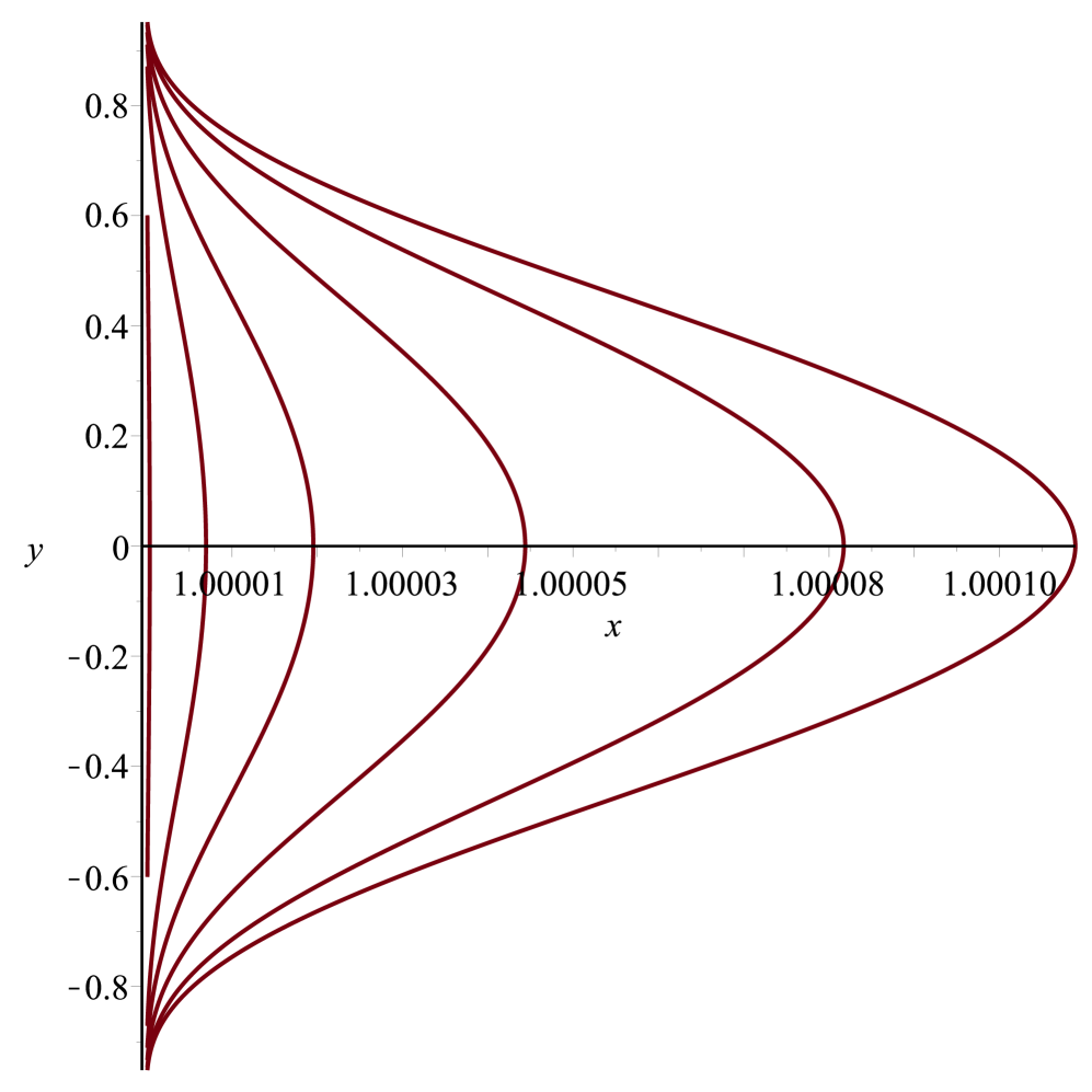
Figure 1: Chronosphere boundary for $q=.5,\,.6,\,.7,\,.8,\,.9,\,.9999$ (from left to right).

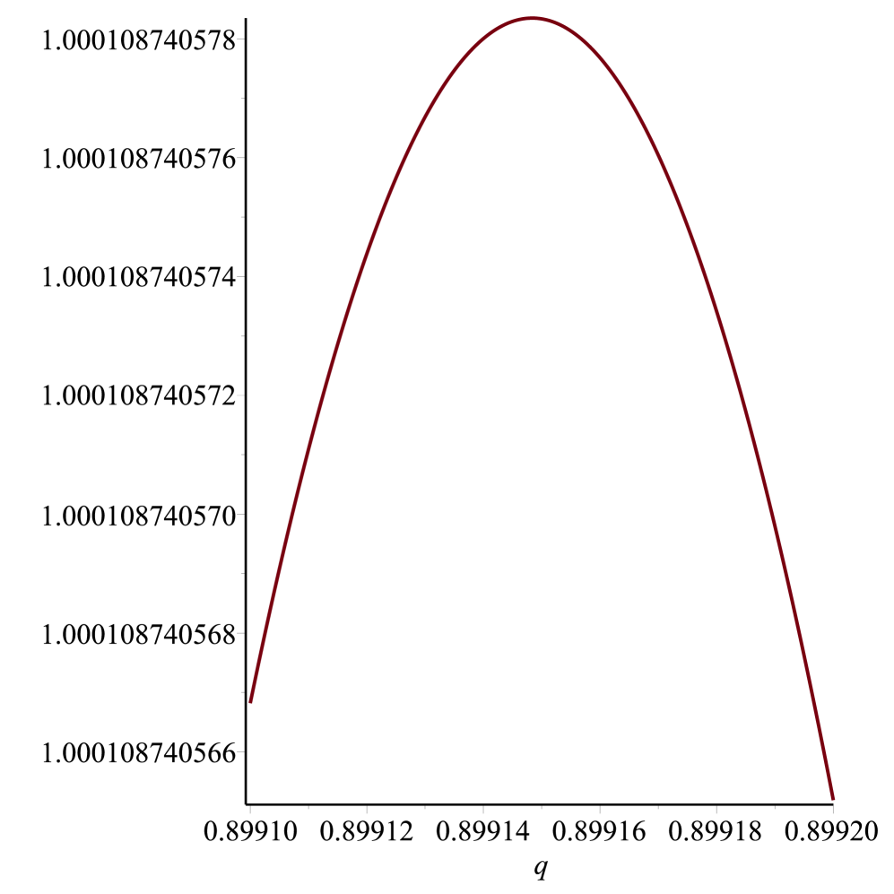
Figure 2: Chronosphere boundary at the equatorial plane (maximal extension) in the vicinity of the critical $q=q^{*}\approx.89915$ corresponding to the maximal size.

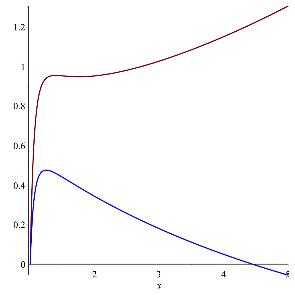
Figure 3: Plots of $10^{-2}g_{\varphi\varphi}$ (black) and $g_{tt}$ (blue) for $q=q^{*}$ at the equatorial plane. $g_{tt}$ changes sign to positive at the ergosphere boundary. Inside the ergosphere $g_{\varphi\varphi}$ seems positive too, but in fact it changes sign at the chronosphere boundary, as can be seen with better resolution near $x=1$ (Fig. 4).

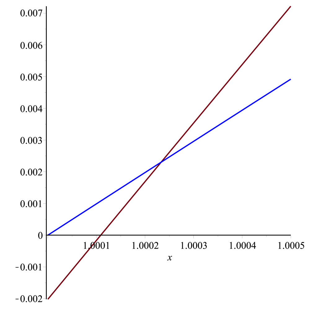
Figure 4: The blow up of the plot Fig. 3 in the vicinity of $x=1$. Intersection of zero by $g_{\varphi\varphi}$ (black) marks the boundary of the chronosphere, inside which $g_{tt}$ (blue) is still positive. Thus the chronosphere lies entirely inside the ergoregion.

The frame dragging velocities $\Omega_{\pm}$ are plotted for $y=0$ and $q=q^{*}$ in Fig. 5 as functions of $x$ in the ergosphere outside the chronosphere. Both are positive there. $\Omega_{+}$ diverges at the chronosphere boundary as $x\to x_{c}+0$ while $\Omega_{-}$ remains bounded,

$$\lim_{x\to x_{c}-0}\Omega_{-}(x)=\frac{g_{tt}}{2\left|g_{t\varphi}\right|}\Big{|}_{x=x_{c}}=\frac{1}{2\omega}\Big{|}_{x=x_{c}}.$$ (3.33)

Inside the chronosphere, $\Omega_{+}\to-\infty$ as $x\to x_{c}-0$, so that now $\Omega_{+}<\Omega_{-}$.

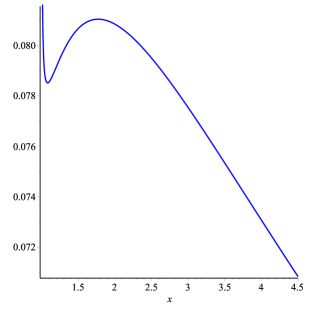
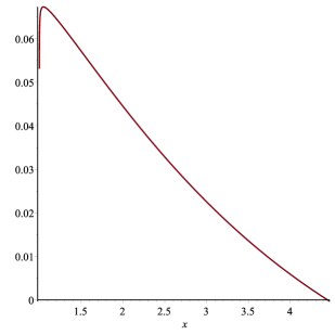
Figure 5: Bounds of dragging angular velocities in the ergosphere outside the chronosphere at the equatorial plane: $\Omega_{+}$ (left panel) and $\Omega_{-}$ (right panel).

Thus the conditions for an observer’s world-line to remain time-like inside the chronosphere are somewhat similar to (3.15), but with an “and” replaced by an “or”,

$$\Omega<\Omega_{+}\,,\quad{\rm or}\quad\Omega>\Omega_{-}\,.$$ (3.34)

We expect that, similarly to the cases studied in RTN ; NW , all possible closed time-like curves inside the chronosphere can be shown to be non-geodesic. One can also argue that typical quantum effects would be expected to be of the order of $1/\kappa$, i.e. one in the above units. The classical chronosphere having a size four orders of magnitude smaller would then be far outside the validity of the classical theory. This can be contrasted with the case of the Taub-NUT metric, where the chronosphere around the Misner string in non-compact, and whose characteristic size is of the order of the horizon radius.

The relative positions of the ergosphere, chronosphere, horizons and string singularity are shown in Fig. 6.

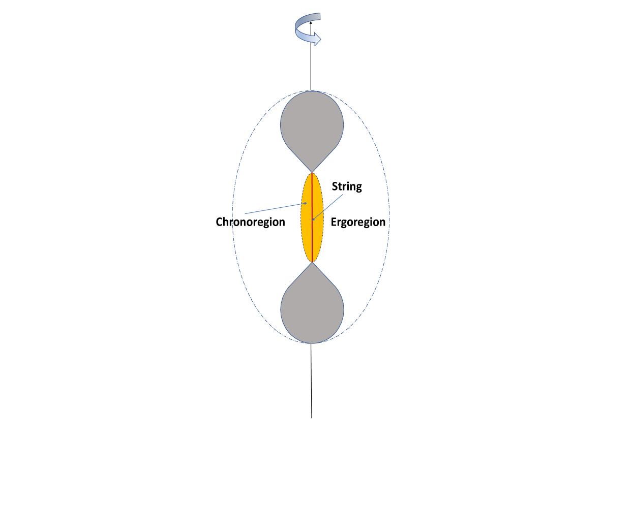
Figure 6: Relative positions of the ergosphere, chronosphere, constituent black holes and string singularity.

In the Kerr metric the chronosphere exists too but it lies inside the event horizon, and thus is ignored. In the case of the TS2 solution, closer to ours, the chronosphere is not inside the ergosphere. The ergoregion there has an inner boundary within which sits the chronosphere. The two surfaces intersect on a singular ring, which is a strong curvature singularity Kodama:2003ch .

III.6 Singular string

This is the segment $x=1$, $-1<y<1$ ($\rho=0$, $-\kappa<z<\kappa$) between the two horizons. For $\xi^{2}\equiv x^{2}-1\to 0$ (with $y^{2}<1$), the solution (2.16)-(2.24) reduces to:

$$ds^{2} \sim -\frac{\kappa^{2}q^{2}}{4}(1-y^{2})^{2}\,d\varphi^{2}+\frac{\kappa^{2}q^{4}}{p^{2}(1-y^{2})}\left[\frac{dy^{2}}{1-y^{2}}\right.$$ (3.35)

$$\left.+d\xi^{2}+\frac{4p^{2}}{\kappa^{2}q^{6}}\xi^{2}\left(dt-\kappa\left(\frac{\lambda(p)}{q}+q(1-p/2)(1-y^{2})\right)d\varphi\right)^{2}\right]$$

$$A \sim \varepsilon\left[\left(1-\frac{2(1+p)\xi^{2}}{q^{2}(1-y^{2})}\right)dt-\kappa\left(\frac{\gamma(p)}{q}+\frac{q(1-y^{2})}{2}\right)d\varphi\right],$$ (3.36)

where we have neglected irrelevant terms of order $\xi^{2}$ and higher.

The singularity at $\xi=0$ looks like a conical singularity. It would be one if the time coordinate $t$ was periodic with period $T$, and it would disappear altogether for the value of the period $T=\pi\kappa q^{3}/p$. The electromagnetic invariants

$$\frac{1}{2}F^{\mu\nu}F_{\mu\nu}\sim\frac{4p^{2}}{\kappa^{2}q^{6}}[(1+p)^{2}-q^{2}y^{2}],\quad\frac{1}{4\sqrt{|g|}}\varepsilon^{\mu\nu\rho\sigma}F_{\mu\nu}F_{\rho\sigma}\sim-\frac{8p^{2}(1+p)}{\kappa^{2}q^{5}}\,y$$ (3.37)

are finite, as well as the mixed Ricci tensor components, the diagonal components behaving as

$$R^{t}_{t}\sim R^{x}_{x}\sim-R^{\varphi}_{\varphi}\sim-R^{y}_{y}\sim\frac{4p^{2}}{\kappa^{2}q^{6}}[(1+p)^{2}+q^{2}y^{2}],$$ (3.38)

with $R^{\varphi}_{t}\sim R^{x}_{y}\sim 0$, so that the Ricci square scalar

$$R^{\mu\nu}R_{\mu\nu}\sim\frac{64p^{4}}{\kappa^{4}q^{12}}[(1+p)^{2}+q^{2}y^{2}]^{2}$$ (3.39)

stays finite near the singularity. On the string $x=1$ both dragging velocities $\Omega_{\pm}$ tend to zero in accordance with the law

$$\lim_{x\to 1}\Omega_{\mp}\sim\pm\frac{4}{q^{2}}\frac{(x^{2}-1)^{1/2}}{\kappa(1-y^{2})^{3/2}}$$ (3.40)

It follows from (3.34) that in the near-string limit $x\to 1$ all observer angular velocities are allowed, which is the exact opposite of the near-horizon limit, so in this sense the interconnecting string can be viewed as an anti-horizon.

The string geometry becomes more transparent in the horizon co-rotating frame $(t,x,y,\hat{\varphi})$, with $d\hat{\varphi}=d\varphi-\Omega_{H}dt$. The near-string metric (3.35) transforms to

$$ds^{2} \sim q^{4}\left[-\frac{(1-y^{2})^{2}}{4\lambda^{2}(p)}\left(dt+\Omega_{H}^{-1}\,d\hat{\varphi}\right)^{2}\right.$$ (3.41)

$$+ \left.\frac{\kappa^{2}}{p^{2}(1-y^{2})}\left(\frac{dy^{2}}{1-y^{2}}+{d\xi^{2}}+\alpha^{2}\xi^{2}\,d\hat{\varphi}^{2}\right)\right].$$

We recognize in (3.41) the metric of a spinning cosmic string DJH ; GC85 in a curved spacetime, with (negative) tension per unit length $(1-\alpha)/4$, where $\alpha(p)$ is given in (3.27), and “spin” $\Omega_{H}^{-1}/4$, where $\Omega_{H}(p)$ is given in (3.20). In view of the fact that the finite-length string connects two black holes, this spin should actually be interpreted as a gravimagnetic flow along the Misner string connecting two opposite NUT sources at $\rho=0$, $z=\pm\kappa$, with the gravimagnetic potential $\omega/2=N_{+}\cos\theta_{+}+N_{-}\cos\theta_{-}$ where $\cos\theta_{\pm}=\mp 1$ along the string, and $N_{+}=-N_{-}=N_{H}$, where

$$N_{H}=\displaystyle\frac{\kappa\lambda(p)}{4q}.$$ (3.42)

Similarly, the constant contribution $-\varepsilon\kappa\gamma(p)/q$ to $A_{\varphi}$ in (3.36) should be interpreted as the magnetic flow along a Dirac string connecting two opposite monopoles at $z=\pm\kappa$ with magnetic charges $P_{+}=-P_{-}=P_{H}$, where $P_{H}$ is the horizon magnetic charge already given in (3.32). The non-constant contribution gives rise to a magnetic field density $\sqrt{|g|}B^{\xi}=F_{y\varphi}=\varepsilon\kappa qy$, which leads to an intrinsic string magnetic moment

$$\mu_{S}=\frac{1}{4\pi}\int_{-1}^{+1}\sqrt{|g|}B^{\xi}\,z\,2\pi\,dy=\frac{\varepsilon\kappa^{2}q}{3}=\frac{\mu}{3}$$ (3.43)

(to obtain the total magnetic moment $\mu$, the magnetic dipole contribution $2\kappa P_{H}$ and the sum of the horizon magnetic moments should be added to this). Other string observables (mass, angular momentum, electric charge) shall be evaluated in the next section.

IV Komar-Tomimatsu observables

Tomimatsu has shown tom84 that, by using the Ostrogradsky theorem and thef Einstein-Maxwell equations, the Komar mass and angular momentum at infinity

$$M=\frac{1}{4\pi}\oint_{\infty}D^{\nu}k^{\mu}d\Sigma_{\mu\nu},\quad J=-(1/8\pi)\oint_{\infty}D^{\nu}m^{\mu}d\Sigma_{\mu\nu}$$ (4.1)

($k^{\mu}=\delta^{\mu}_{t}$, $m^{\mu}=\delta^{\mu}_{\varphi}$) can be transformed into the sums over the boundary surfaces $S_{n}$ (here, the two horizons and the string) $M=\sum_{n}M_{n}$, $J=\sum_{n}J_{n}$, with

$$M_{n} = \frac{1}{8\pi}\oint_{S_{n}}\left[g^{ij}g^{ta}\partial_{j}g_{ta}+2(A_{t}F^{it}-A_{\varphi}F^{i\varphi})\right]d\Sigma_{i}.$$

$$J_{n} = -\frac{1}{16\pi}\oint_{S_{n}}\left[g^{ij}g^{ta}\partial_{j}g_{\varphi a}+4A_{\varphi}F^{it}\right]d\Sigma_{i}.$$ (4.2)

In the case of rotating black holes, the horizon Komar mass and angular momentum ((IV) with $S_{n}=H$) reduce on the horizons to tom84 ; smarr

$$M_{H} = \frac{1}{8\pi}\oint_{H}\left[\omega\partial_{z}{\rm Im}{\cal E}+2\partial_{z}(A_{\varphi}\,{\rm Im}\psi)\right]dz\,d\varphi,$$ (4.3)

$$J_{H} = \frac{1}{8\pi}\oint_{H}\omega\left[-1+\displaystyle\frac{1}{2}\omega\,\partial_{z}{\rm Im}{\cal E}+\partial_{z}(A_{\varphi}\,{\rm Im}\psi)+\omega\hat{A}_{t}\partial_{z}{\rm Im}\psi\right]dz\,d\varphi$$ (4.4)

(the second term in (4.3) was omitted in tom84 ).

Transforming from the Weyl coordinates $\rho,z$ to the coordinates $X,Y$, and taking into account the constancy of $\omega$ and $\hat{A}_{t}$ over the horizon, the expressions (4.3) and (4.4) can be integrated to

$$M_{H} = \frac{1}{4}\bigg{[}\omega{\rm Im}{\cal E}+2A_{\varphi}\,{\rm Im}\psi\bigg{]}_{X=\infty}^{X=0},$$ (4.5)

$$J_{H} = \frac{1}{4}\omega\left[\displaystyle\frac{1}{2}\omega{\rm Im}{\cal E}+A_{\varphi}\,{\rm Im}\psi+\omega\hat{A}_{t}{\rm Im}\psi\right]_{X=\infty}^{X=0},$$ (4.6)

evaluated over the upper horizon $Y=1$ (the contributions of the two horizons are equal). Using $\omega_{H}=1/\Omega_{H}$, we find

$$M_{H_{\pm}}= \frac{\kappa}{p}+\frac{\kappa p}{2},$$ (4.7)

$$J_{H_{\pm}}= \frac{\kappa^{2}}{8qp}\left[2\lambda(p)(2+p^{2})+q^{2}p(1+p)(2-p)\right].$$ (4.8)

The horizon mass (4.7) is larger than half of the global mass $2\kappa/p$, so the string must have negative mass.

Similarly, the horizon electric charge

$$Q_{H}=\frac{1}{4\pi}\int_{H}\sqrt{|g|}F^{t\rho}dzd\varphi$$ (4.9)

may be transformed into the Tomimatsu integral tom84

$$Q_{H}=-\displaystyle\frac{1}{4\pi}\oint_{H}\omega\,d\,{\rm Im}\psi\,d\varphi,$$ (4.10)

leading to

$$Q_{H_{\pm}}=-\displaystyle\frac{\varepsilon\kappa(1+p)}{2}.$$ (4.11)

To ensure global electric neutrality, the string must be also charged, which we shall now check.

The near-string covariant component $F_{t\xi}$ of the radial electric field vanishes to order ${\rm O}(\xi)$, but on account of $g_{tt}={\rm O}(\xi^{2})$ and $\sqrt{|g|}={\rm O}(\xi)$, the radial electric field density $\sqrt{|g|}F^{t\xi}$ is finite and constant along (a small cylinder centered on) the string, leading to the electric charge

$$Q_{S}=\frac{1}{4\pi}\int_{-1}^{+1}\sqrt{|g|}F^{t\xi}\,2\pi\,dy=\varepsilon\kappa(1+p).$$ (4.12)

This string electric charge together with the horizon electric charges lead to a vanishing total electric charge

$$Q_{H_{+}}+Q_{H_{-}}+Q_{S}=0,$$ (4.13)

a vanishing electric dipole moment, and a contribution to the total electric quadrupole moment, to which must be added that of the two opposite horizon electric dipole moments generated by the rotation of the horizon magnetic charges, and the sum of the horizon electric quadrupole moments.

The string mass and angular momentum can be evaluated from (IV) integrated over a small cylinder centered on the string $x=1$, $-1<y<1$, and are the sum of gravitational and electromagnetic contributions. Although, in the co-rotating frame, the string is a spinning cosmic string with negative tension, and thus presumably negative gravitational mass, in the global frame the gravitational contribution to the string mass is – surprisingly – positive. However it is overwhelmed by the negative electromagnetic contribution $-Q_{S}A_{t}(\xi=0)$, resulting in a net negative string mass

$$M_{S}=\kappa-\kappa(1+p)=-\kappa p,$$ (4.14)

which represents the binding energy between the two black holes of mass $(\kappa/p+\kappa p/2)$, leading to the total mass

$$M=M_{H_{+}}+M_{H_{-}}+M_{S}=\frac{2\kappa}{p}.$$ (4.15)

The fact that the string mass is negative explains the repulsion experienced by test particles in geodesic motion near the string (antigravity).

Similarly, the string angular momentum is the sum of gravitational and electromagnetic contributions

$$J_{S} = \kappa^{2}\left[\frac{\lambda(p)}{2q}+\frac{q}{3}\left(1-\frac{p}{2}\right)\right]-\kappa^{2}(1+p)\left[\frac{\gamma(p)}{q}+\frac{q}{3}\right]$$ (4.16)

$$= \frac{\kappa^{2}}{2q}\left[\lambda(p)-2(1+p)\gamma(p)-pq^{2}\right].$$

The first term $\kappa^{2}\lambda(p)/2q$ is the NUT dipole $2\kappa N_{H}$. The second term can be understood as the charge-monopole angular momentum contribution $Q_{S}(P_{H_{+}}-P_{H_{-}})$. If this interpretation is correct, the remainder $-\kappa pq/2$ corresponds to the intrinsic string angular momentum. It can be checked that the horizon angular momenta (4.8) and the total string angular momentum (4.16) add up to the net angular momentum (3.5):

$$J=J_{H+}+J_{H_{-}}+J_{S}=\frac{\kappa^{2}q(4+p^{2})}{p^{2}}.$$ (4.17)

V Geodesics

Two obvious first integrals of the geodesic equations of motion are

$$F\left(\dot{t}-\omega\dot{\varphi}\right)=E,$$ (5.1)

$$F^{-1}\rho^{2}\dot{\varphi}+F\omega\left(\dot{t}-\omega\dot{\varphi}\right)=L,$$ (5.2)

where $\dot{=}d/d\tau$, and $E$ (energy) and $L$ (orbital angular momentum) are two constants of the motion. A third first integral is

$$\frac{ds^{2}}{d\tau^{2}}\equiv g_{\mu\nu}\dot{x}^{\mu}\dot{x}^{\nu}\equiv T+U=\epsilon,$$ (5.3)

where $\epsilon=-1$, $0$ or $+1$ for timelike, null or spacelike geodesics, and

$$T = \kappa^{2}\Sigma e^{2\nu}\left(\displaystyle\frac{\dot{x}^{2}}{x^{2}-1}+\displaystyle\frac{\dot{y}^{2}}{1-y^{2}}\right)>0,$$ (5.4)

$$U = \displaystyle\frac{(L-E\omega)^{2}F}{\rho^{2}}-\displaystyle\frac{E^{2}}{F}.$$ (5.5)

The fourth equation is the geodesic equation for the coordinate $y$, which reads:

$$\frac{2\kappa^{2}}{\sqrt{1-y^{2}}}\frac{d}{d\tau}\left(\frac{\Sigma e^{2\nu}\dot{y}}{\sqrt{1-y^{2}}}\right)=\frac{E^{2}\Sigma}{f}\left[2\frac{\Sigma_{y}}{\Sigma}+2\nu_{y}-\frac{f_{y}}{f}\right]+\frac{2\kappa E\Pi}{f}\left[\frac{\Pi_{y}}{\Pi}-\frac{f_{y}}{f}\right]$$

$$+\epsilon\left[\frac{\Sigma_{y}}{\Sigma}+2\nu_{y}\right]-\frac{(Lf-\kappa E\Pi)^{2}}{\kappa^{2}f\Sigma(x^{2}-1)(1-y^{2})}\left[\frac{f_{y}}{f}+2\frac{y}{1-y^{2}}+2\nu_{y}\right],$$ (5.6)

where $\rho^{2}$ is given by Eq. (2.3), $F_{y}=\partial F/\partial y$ and so on.

Contrary to the Kerr case, there is no Carter constant corresponding to the second order Killing tensor, so the system of $(x(\tau),\,y(\tau))$ equations cannot be decoupled. However one can derive a separate non-linear differential equation for the function $y(x)$ describing the geodesic trajectories in the $(x,\,y)$ plane. In the ZV2 case such an equation was given in Kodama:2003ch . To this aim one writes $\dot{y}=y^{\prime}\dot{x}$, where $y^{\prime}=dy/dx$, and substitute this in the Eqs. (5.3, 5.4):

$$\kappa^{2}\Sigma e^{2\nu}{\dot{x}^{2}}\left(\displaystyle\frac{1}{x^{2}-1}+\displaystyle\frac{{y^{\prime}}^{2}}{1-y^{2}}\right)+U=\epsilon\,,$$ (5.7)

to express $\dot{x}^{2}$ as a function of three variables $\chi(x,y,y^{\prime})$:

$$\dot{x}^{2}=\chi\equiv\frac{(\epsilon-U)(x^{2}-1)(1-y^{2})}{\kappa^{2}\Sigma e^{2\nu}\left[1-y^{2}+(x^{2}-1)y^{\prime 2}\right]}\,.$$ (5.8)

Making the same substitution in Eq. (V) we obtain the desired equation

$$y^{\prime\prime}\left(\chi+y^{\prime}\chi_{y^{\prime}}/2\right)+y^{\prime}(\partial_{x}+y^{\prime}\partial_{y})\ln\left(\Sigma e^{2\nu}\chi^{1/2}\right)+2yy^{\prime 2}\chi(1-y^{2})^{-1}=\Phi(1-y^{2})/2\kappa^{2}\,.$$ (5.9)

Let us first discuss the behavior of geodesics near the string $S$ ($x=1$, $y^{2}<1$). We have seen that near $S$ both $F^{-1}\rho^{2}$ and $\omega$ go to finite limits depending on $y$, so that the first centrifugal term in $U$ is negative and bounded, while from (3.35) the second term $-E^{2}/F$ is positive and increases without bound, so that the geodesics are reflected by a potential barrier. This argument breaks down in the exceptional case $E=0$, where only the (attractive) centrifugal potential remains, so that these geodesics terminate (or originate) on the singularity $S$. However, the timelike or null geodesics ($\epsilon\leq 0$) are confined to the region where the centrifugal potential is attractive, i.e. inside the ergosphere, and the orbits must have a turning point somewhere, and by reason of symmetry end again on the singularity.

Consider now geodesics approaching either of the two points $H_{\pm}$ ($x=1$, $y=\pm 1$). The simplest case is that of axial geodesics $\rho\texttwosuperior=0$. A first possibility is $y=\pm 1$ (axial geodesics originating from infinity), which necessitates $L=0$, and in which case $\omega=0$. Then $fe^{2\nu}=x^{2}-1$, so that Eq. (5.3) reduces to the exact equation

$$\dot{x}^{2}-\frac{\epsilon p^{2}(x^{2}-1)^{2}}{4\kappa^{2}x^{2}\Sigma(x)}=\frac{E^{2}}{\kappa^{2}},$$ (5.10)

where $\Sigma(x)$ goes to a finite limit for $x\to 1$ . Clearly these special geodesics attain $x=1$ in a finite affine time, with an affine velocity equal to that of light, and can be analytically continued to $x<1$, all the way to $x\to-\infty$ (from (2.19) $x^{2}\Sigma(x)$ admits the lower bound $p^{2}/2$). The other possibility is $x=1$ (geodesics along the string from one horizon to the other). Then $F=0$, so finiteness of $U$ requires $E=0$, the first integrated geodesic equation

$$\dot{y}^{2}-\frac{\epsilon p^{2}}{\kappa^{2}q^{4}}(1-y^{2})^{2}=\frac{4L^{2}p^{2}}{\kappa^{4}q^{6}}$$ (5.11)

showing that the two horizon components are connected by axial spacelike geodesics, null geodesics with $L\neq 0$, as well as timelike geodesics with $|L|>\kappa q/2$.

In the generic case, let us assume that the geodesic hits the point $H_{\pm}$ tangentially to the curve

$$1-y^{2}=X^{2}(x^{2}-1),$$ (5.12)

i.e. that the initial conditions for the orbit $y(x)$ at $x=1$ are $y(1)=\pm 1$, $y^{\prime}(1)=\mp X^{2}$, and show that these conditions are consistent with the geodesic equation for $y$ (V). First we observe that, as $x^{2}\to 1$, the functions $f$, $\Sigma$ and $\Pi$ all go to finite limits (given below in (III.4)), while the logarithmic derivatives $\Sigma_{y}/\Sigma$, $\nu_{y}$ and $f_{y}/f$ are all of order $1/(x^{2}-1)$. It follows that the right-hand side of (V) is dominated by the last term. Furthermore, $f\sim-q^{2}x^{2}(1-y^{2})/(x^{2}-1)$, so that to leading order $f/(1-y^{2})$ does not depend on $y$, and the square bracket in this last term is dominated by the term $2\nu_{y}$. Accordingly, near $x=1$ Eq. (V) may be replaced to leading order by

$$\frac{2\kappa^{2}}{\sqrt{1-y^{2}}}\left(\frac{\Sigma e^{2\nu}\dot{y}}{\sqrt{1-y^{2}}}\right)^{\dot{}}\simeq-2\displaystyle\frac{(L-E\omega)^{2}F}{\rho^{2}}\nu_{y}\simeq-2U\nu_{y}\simeq 2T\nu_{y},$$ (5.13)

where we have used (5.5) and (5.3) to leading order. Because $\Sigma$ and $\dot{y}$ go to finite limits for $x\to 1$, their derivatives may be neglected in (5.13), which may be again replaced by

$$2\kappa^{2}\Sigma e^{2\nu}\,\frac{\dot{y}}{1-y^{2}}\left[2\dot{\nu}+\frac{y\dot{y}}{1-y^{2}}\right]\simeq 2T\nu_{y}.$$ (5.14)

Comparing with the definition (5.4) of $T$, we arrive at the equation

$$-2(x^{2}-1)(\nu_{x}-X^{2}y\nu_{y})+1\simeq(x^{2}-1)(1+X^{2})y\nu_{y},$$ (5.15)

which, using the partial derivatives of (2.20)

$$\nu_{x}\simeq\left(2-\frac{3}{1+X^{2}}\right)\frac{1}{x^{2}-1},\qquad\nu_{y}\simeq\frac{3y}{1+X^{2}}\frac{1}{x^{2}-1},$$ (5.16)

is seen to be satisfied. This shows that the behavior (2.20) of the metric function $e^{2\nu}$, inherited from the ZV2 solution, is essential for the consistency of the assumption (5.12).

Considering now the effective radial equation $T\sim-U$ where $y(x)$ is given by (5.12) and $U$ is dominated by the negative centrifugal contribution, and using the limit

$$\lim_{x\to 1}{\displaystyle\frac{e^{2\nu}\rho^{2}}{x^{2}-1}}=\displaystyle\frac{4\kappa^{2}}{p^{2}}\,\displaystyle\frac{X^{2}}{(1+X^{2})^{3}},$$ (5.17)

we see that the ‘radial’ velocity $\dot{x}$ goes for $x\to 1$ to a finite limit

$$\dot{x}_{H}=-\frac{p(qL+\kappa\lambda(p)E)}{2\kappa^{2}}\,\frac{1+X^{2}}{\Sigma_{H}(X)}.$$ (5.18)

The axial radial velocity $-E/\kappa$ is recovered in the limit ($X\to 0$, $L\to 0$).

The geodesic equations being analytical in $x$ and $y$, these geodesics can be smoothly continued through the horizon $x=\pm y=1$ to an interior region with $x<1$ and $y^{2}>1$, without changing the signature of the metric because the simultaneous sign change of $x^{2}-1$ and $1-y^{2}$ leads to a sign change of $e^{2\nu}$, proportional to $x^{2}-y^{2}$.

VI Beyond the horizons

The metric inside the black hole (region $II$) is again given by (2.16) where now $-1<x<1$ and $y\geq 1$ (North interior region $II_{+}$) or $y\leq-1$ (South interior region $II_{-}$). These two isometrical interior regions are actually disconnected, each being bounded by two horizons $H_{\pm}$ ($x=1,\,y=\pm 1$) and $H^{\prime}_{\pm}$ ($x=-1,\,y=\pm 1$). Behind the second horizons $H^{\prime}_{\pm}$ lie two new exterior regions with $x<-1$ and $-1\leq y\leq 1$. In the most economical maximal analytic extension, these two isometrical regions can be identified (exterior region $III$).

In region $II$ the role of the radial coordinate is now played by $y$, $x$ being related to the natural angular coordinate by $x=\cos\theta$. It follows that the coordinate singularity at ($x=1$, $|y|>1$) as well as that at ($x=-1$, $|y|>1$) are axial singularities of the cosmic string type, the near-singularity metric and electromagnetic potential, obtained by taking $1-x^{2}=\xi^{2}\to 0$ being now

$$ds^{2} \sim -\frac{\kappa^{2}q^{2}}{4}(y^{2}-1)^{2}\,d\varphi^{2}+\frac{\kappa^{2}q^{4}}{p^{2}(y^{2}-1)}\left[\frac{dy^{2}}{y^{2}-1}\right.$$ (6.1)

$$\left.+d\xi^{2}+\alpha^{2}\Omega_{H}^{2}\xi^{2}\left(dt-\kappa\left(\frac{\lambda(\pm p)}{q}-q(1\mp p/2)(y^{2}-1)\right)d\varphi\right)^{2}\right]$$

$$A \sim \varepsilon\left[\left(1-\frac{2(1\pm p)\xi^{2}}{q^{2}(y^{2}-1)}\right)dt-\kappa\left(\frac{\gamma(\pm p)}{q}-\frac{q(y^{2}-1)}{2}\right)d\varphi\right],$$ (6.2)

These two strings have different tensions $(1-\alpha(\pm p))/4$ and different spins $\Omega_{H}(\pm p)^{-1}/4$ (it is clear from (II.3) that the exchange $x\to-x$ is equivalent to the exchange $p\to-p$), $\alpha(\pm p)$ being given in (3.27) and $\Omega_{H}(\pm p)$ in (3.20) (with the product $\alpha(\pm p)\Omega_{H}(\pm p)=\mp 2p/\kappa q^{3}$). As in the case of Sect. 4, the effective potential of (5.3) increases for $E\neq 0$ as $1/\xi^{2}$, so that no geodesics can reach these singular strings, except for exceptional geodesics with $E=0$. Again, these cosmic strings are themselves geodesic with $E=0$ and the first integrated geodesic equation (5.11).

There is also an apparent singularity at $x=0$. However evaluation of the various metric elements near $x=0$ leads to the regular behavior

$$ds^{2} \sim -\frac{1}{1+q^{2}y^{2}}\left[dt+\frac{4\kappa q}{p}\left(1+\frac{q^{2}}{8}(y^{2}-1)\right)(y^{2}-1)d\varphi\right]^{2}$$ (6.3)

$$+ \kappa^{2}(1+q^{2}y^{2})\left[y^{-6}\left(dx^{2}+\frac{dy^{2}}{y^{2}-1}\right)+(y^{2}-1)d\varphi^{2}\right].$$

Again, there is no ring singularity in region $II$, because $\Sigma$ is the sum of two squares, the second of which can vanish only for $x=p/2$, and it is then easy to show that $\Sigma(p/2,y)>4$.

The metric is by construction regular for $y=\pm 1$, being of the form

$$ds^{2}\sim-\frac{f(x)}{\Sigma(x)}\,dt+\frac{\kappa^{2}\Sigma(x)(1-x^{2})}{f(x)}\left[\frac{dx^{2}}{1-x^{2}}+\frac{dy^{2}}{y^{2}-1}+(y^{2}-1)d\varphi^{2}\right],$$ (6.4)

with $f(x)$ strictly positive. Axial ($l=0$) geodesics along $y=\pm 1$ connect the two horizons in region $II$, the first integrated geodesic equation being (5.10). For timelike axial geodesics, it seems (see Appendix C) that the effective potential $V(x)$ has a relative maximum in the range $x\in[-1,0]$ with $V_{max}>V(\infty)=1/\kappa^{2}$. So an observer radially infalling from $x=+\infty$ with sufficiently high velocity will cross the two horizons and proceed towards $x=-\infty$ in region $III$, but an observer with sufficiently low velocity will instead be reflected back through the outer horizon to $x=+\infty$, albeit in another spacetime coordinate patch $I$, to the future of the previous one. The effective radial distance between the two horizons in region $II$ is $\Delta r=\kappa\Delta x=2\kappa=pM$.

When $|y|$ increases, an ergosurface $f(x,y)=0$ appears. The behaviors of the various metric and electromagnetic functions for $y^{2}\to\infty$

$$f \sim -\frac{q^{2}x^{2}y^{2}}{1-x^{2}},\quad\Sigma\sim\overline{v}\sim\frac{q^{4}y^{4}}{4(1-x^{2})^{2}},\quad-e^{2\nu}\sim\frac{4x^{2}(1-x^{2})^{2}}{p^{2}y^{6}},$$

$$\Pi \sim \Pi_{2}(x)y^{4},\quad\Theta\sim\frac{q^{5}y^{6}}{8x(1-x^{2})^{2}}$$ (6.5)

lead to the non-asymptotically flat behavior of the metric and electromagnetic field

$$ds^{2} \sim -\frac{\kappa^{2}q^{2}y^{4}}{4x^{2}}d\varphi^{2}+\frac{\kappa^{2}q^{4}x^{2}}{p^{2}y^{2}}\left(\frac{dy^{2}}{y^{2}}+\frac{dx^{2}}{1-x^{2}}+\right.$$ (6.6)

$$+ \left.\frac{4p^{2}(1-x^{2})}{\kappa^{2}q^{6}}\left[dt+\frac{\kappa\Pi_{2}(x)(1-x^{2})y^{2}}{q^{2}x^{2}}d\varphi\right]^{2}\right),$$

$$A \sim \varepsilon\left\{\left[1+\frac{(1-x^{2})(p-6x-3px^{2}+4x^{3})}{q^{2}xy^{2}}\right]dt+\frac{\kappa qy^{2}}{2x}\,d\varphi\right\}.$$ (6.7)

The squared Ricci scalar diverges as $y^{4}$.

As it is enclosed between two horizons which are topological spheres, the singularity $|y|\to\infty$ must actually be at finite distance. Indeed, putting $y=\zeta^{-1}$ and $x=\cos\chi$, the asymptotic metric (6.6) takes the form

$$ds^{2} \simeq -\frac{\kappa^{2}q^{2}}{4\cos^{2}\chi}\zeta^{-4}\,d\varphi^{2}+\frac{\kappa^{2}q^{4}\cos^{2}\chi}{p^{2}}\left[d\zeta^{2}+\zeta^{2}\,d\chi^{2}\right.$$ (6.8)

$$+ \left.\frac{4p^{2}\zeta^{2}}{\kappa^{2}q^{6}}\sin^{2}\chi(dt+\frac{\kappa\Pi_{2}(\chi)\sin^{2}\chi}{\zeta}^{-2}d\varphi^{2})\right],$$

It follows that $\zeta=0$ corresponds to a point $S_{0}$ in the $\varphi=$ constant sections, or a closed timelike line of the four-dimensional spacetime. Note also that $\sqrt{|g|}$ goes to the finite limit $(\kappa^{3}q^{4}/p^{2})\cos^{2}\chi|\sin\chi|$ for $\zeta\to 0$, so that this singularity has a finite volume per unit time $(4\pi/3)\kappa^{3}q^{4}/p^{2}$.

For $E\neq 0$, the effective potential $U$ is dominated by the term $-E^{2}/F$, which is positive and increases as $y^{2}$, so that the geodesics turn back before reaching $y\to\infty$. For $E=0$, however, $U=L^{2}F/\rho^{2}$ is negative and goes to zero as $y^{-4}$, so that timelike geodesics again turn back while null geodesics extend to infinity and are complete ($\tau\propto y$). Thus only spacelike geodesics with $E=0$ terminate at the singularity $S_{0}$. This analysis applies equally to geodesics following the cosmic strings $x=1$ and $x=-1$. Indeed, analytic extension of the geodesic motion through the two exterior horizons $H_{+}$ and $H_{-}$ shows that the line $x=1$ may be viewed as a single cosmic string connecting the two singularities $S_{0\pm}$. Likewise, the line $x=-1$ may be considered as a single cosmic string connecting the two singularities $S_{0\pm}$ through the two interior horizons $H^{\prime}_{+}$ and $H^{\prime}_{-}$, these singularities themselves arising from the mismatch between the different tensions and angular velocities of the two cosmic strings. These cosmic strings are also Dirac and Misner strings, the exterior cosmic string carrying the magnetic and gravimagnetic fluxes computed in Sect. 3, and the interior cosmic string carrying the corresponding fluxes with $p$ replaced by $-p$. It follows that the singularities $S_{0\pm}$ have opposite magnetic charges $\pm P_{0}$ and NUT charges $\pm N_{0}$ with

$$P_{0}=\frac{\varepsilon\kappa}{2q}[\gamma(p)-\gamma(-p)]=\frac{\varepsilon\kappa}{q}(3+p^{2}),\quad N_{0}=\frac{\kappa}{4q}[\lambda(p)-\lambda(-p)]=\frac{\kappa}{q}(1+p^{2}).$$ (6.9)

Fig. 7 shows the relative positions of the two outer and inner horizons, the connecting strings in regions $I$ and $II_{\pm}$, and the singularities $S_{0\pm}$.

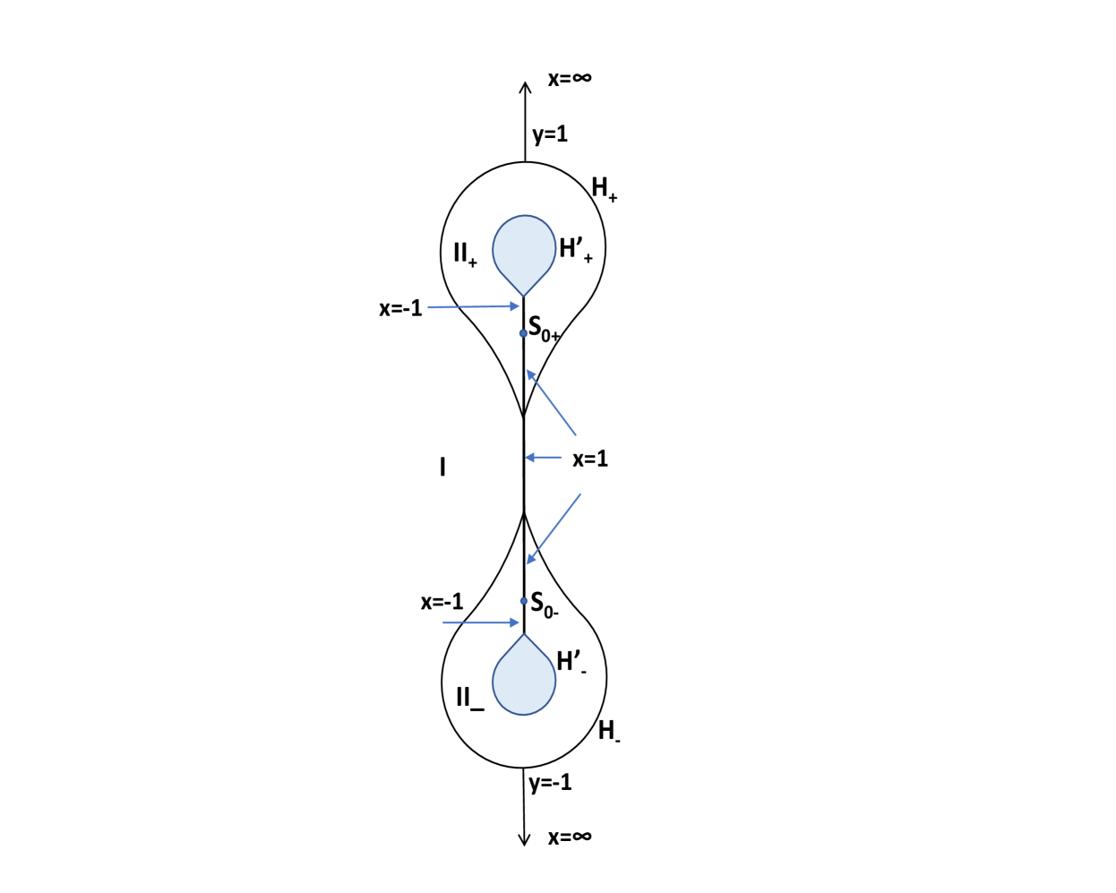
Figure 7: Relative positions of the two outer and inner horizons, the connecting strings in regions $I$ and $II_{\pm}$, and the singularities $S_{0\pm}$.

The properties of the third region $III$ ($x<-1$ and $-1\leq y\leq 1$) are in the whole similar to those of the exterior region $I$, except for the existence of the ring singularity $\Sigma(x,y)=0$, i.e. $y=0$ and $x=x_{0}$ with

$$\frac{p(x_{0}^{2}+1)}{2x_{0}}+1+\frac{q^{2}}{2(x_{0}^{2}-1)}=0.$$ (6.10)

We show in Appendix C that, for every $p\in]0,1[$, this equation has a solution $x_{0}(p)<-1$. This is actually such that $x_{0}(p)<-1/p$ . To the difference of the case of Kerr, $f(x_{0},0)$ does not vanish. Using (6.10), one can show that

$$f(x_{0},0)=\frac{(px_{0}^{2}+2x_{0}+p)^{2}}{4x^{2}}>0,$$ (6.11)

so that the equatorial ring singularity is timelike. From (5.5) the effective potential $U$ diverges on the ring, so that all geodesics are generically repelled away from the ring by a potential barrier. The only geodesics which can reach the ring are spacelike geodesics with parameters fine-tuned so that $L/E=\kappa\Pi(x_{0})/f(x_{0})$, in which case $L-E\omega$ goes to zero as $x-x_{0}$, so that $U$ goes on the ring to a constant positive value $U_{0}$. Note also that on this ring $g_{\varphi\varphi}\sim-\kappa^{2}\Pi^{2}/\Sigma f\to-\infty$. As a consequence, $g_{\varphi\varphi}$ must be negative in the vicinity of the ring, which therefore lies within the region of CTCs.

If the two innermost regions $III$ are identified, the spatial topology of the maximally extended spacetime can be described, in terms of the coordinates $X$ (or $\eta=2\arctan{X}$) and $Y$ previously introduced, as that of a truncated cylinder, with longitudinal coordinate $X\geq 0$ ($0\leq\eta\leq\pi$) and angular coordinate $\psi$ related to $Y$ by $Y=\tan\psi$, see Fig. 8.

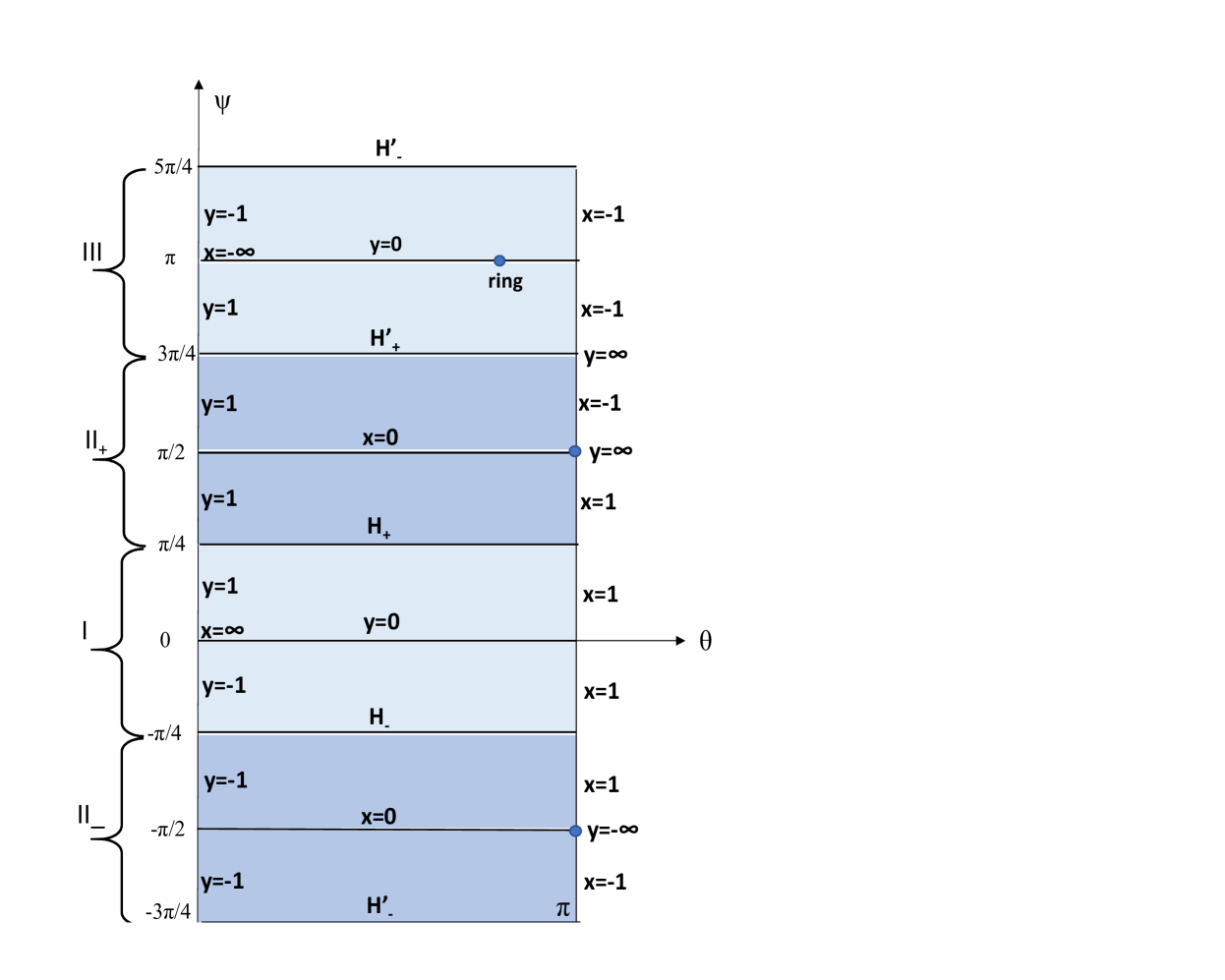
Figure 8: Spatial topology of the two-black hole system, with the outer regions $I$ and $III$ and inner regions $II_{\pm}$. The horizons $H_{\pm}$ and $H^{\prime}_{\pm}$ are represented by horizontal lines, the two regular $z$ axes by the left vertical line, and the two singular strings by the right vertical line.

The basis circle $X=0$ ($\eta=0$) corresponds to the regular portion of the symmetry axis, $y^{2}=1$, except for the two points $\psi=0$ ($x\to+\infty$) and $\psi=\pi$ ($x\to-\infty$) which correspond to spacelike infinity. So the regular portion of the symmetry axis has two components, each homeomorphic to the real line. The generatrices $\psi=0$ or $\psi=\pi$ correspond to the equatorial plane. The horizons are represented by the generatrices $\psi=\pi/4+k\pi/2$, the sector $\psi\in]-\pi/4,\pi/4[$ corresponding to region $I$, the sector $\psi\in]\pi/4,3\pi/4[$ to region $II_{+}$, the sector $\psi\in]3\pi/4,5\pi/4[$ to region $III$, and the sector $\psi\in]5\pi/4,7\pi/4[$ to region $II_{-}$. The circle $X\to\infty$ ($\eta=\pi$) corresponds to the singular cosmic strings $x^{2}=1$ connecting together, through the two exterior or interior horizon conical singularities, the two singular points $S_{0\pm}$ ($X\to\infty$, $\psi=\pm\pi/2$) which correspond to the timelike singularities $y\to\pm\infty$ in regions $II_{\pm}$. Finally, the isolated timelike singular ring $(x=x_{0},y=0)$ is represented by a point $X=X_{0}$ on the generatrix $\psi=\pi$.

The metric function $f=-||\partial/\partial t||^{2}$ is positive on the basis circle $X=0$, while it is negative on the horizons $\psi=\pi/4+k\pi/2$. So the $\varphi=$ constant sections of the ergosurfaces are represented by curves connecting the successive points ($X=0$, $\psi=\pi/4+k\pi/2$), the ergosphere extending from these curves to $X\to\infty$. Conversely, $g_{\varphi\varphi}=||\partial/\partial\varphi||^{2}$ is positive on the horizons and negative on the singular circle $X\to\infty$, so that the causal boundary $g_{\varphi\varphi}=0$ is represented by curves connecting successive points ($X=\to\infty$, $\psi=\pi/4+k\pi/2$), the domain extending from these curves to $X\to\infty$ containing CTCs. Because the singular ring ($X=X_{0}$, $\psi=\pi$) belongs both to the stationary domain $f>0$ and to the domain containing CTCs, the ergosurface and the causal boundary must intersect in region $III$.

VII Conclusions

The binary black hole presented here differs from numerous previously known double-center solutions in many respects. First, it was derived without use of ISM, which is designed to generate solutions with as many independent parameters as possible. This generality, however, creates problems with calculating physical parameters and revealing physical properties of the solutions. Our solution is much more simple and contains only two parameters, which can be chosen as the total mass and the total angular momentum, exactly as in the Kerr case. It was derived using an original generating technique due to one of the authors which is a product of invariance transformations of the dimensionally reduced target space sigma model with a rotation in the space of Killing orbits. Applied to the ZV2 vacuum metric, this procedure leads to a rotating two-center solution of the Einstein-Maxwell equations with many attractive features. Asymptotically it looks like the Kerr solution with zero Coulomb charges but with magnetic dipole and electric quadrupole moments. It has an ergosphere inside which one finds two extremal co-rotating black holes touching the ergosphere at the points on the symmetry axis, endowed with equal electric charges and opposite magnetic and NUT charges. Since the total NUT charge is zero, the metric is asymptotically flat.

Contrary to many known rotating double-center solutions to vacuum and electrovacuum gravity, our solution is manifestly free from ring singularities outside the horizons. Still, the solution is unbalanced and contains conical singularities on the segment of the polar axis between the constituent black holes. This string co-rotates with the horizons, has an electric charge balancing the two black hole charges, and is also the Dirac string carrying the magnetic flux between the opposite magnetic monopoles, and the Misner string carrying the gravimagnetic flux between the opposite NUT charges.

The rotating string is surrounded by a tiny chronosphere which lies entirely inside the ergosphere, its maximal size being of the order of $10^{-4}$ of the length defined by the Schwarzschild mass of the solution. We investigated its structure finding that one of the boundaries of the dragging angular velocity diverges on the chronosphere. Both boundaries of dragging velocities converge on the polar axis to a zero value.

The solution was analytically continued inside the horizons. The most economical maximal analytical extension contains two isometrical interior regions between an outer and an inner horizon (both degenerate). Inside these interior regions one meets a strong closed timelike singularity. Beyond the inner horizons there is a third, asymptotically flat region containing a timelike ring singularity repelling almost all geodesics.

Our family of solutions interpolates between the vacuum ZV2 solution and (after a suitable rescaling) the extreme Kerr metric. Remarkably, the total horizon area of the constituents is, in this extreme limit, one-half of the horizon area of the limiting Kerr black hole of the same mass. This is similar to the case of ZV2: as shown by Kodama and Hikida Kodama:2003ch , the total horizon area of the two constituents is one-half of the area of the Schwarzschild black hole of the same mass. We leave a more complete discussion of thermodynamics for future work.

Appendix A: Positivity of $g_{\varphi\varphi}$ on the ergosurface

Let us show that

$$g_{\varphi\varphi}=\kappa^{2}\left(\frac{\Sigma}{f}(x^{2}-1)(1-y^{2})-\frac{\Pi^{2}}{\Sigma f}\right)$$ (A.1)

is finite on the ergosurface where

$$f(x,y)=\frac{p^{2}(x^{2}-1)^{2}}{4x^{2}}-\frac{q^{2}x^{2}(1-y^{2})}{x^{2}-1}$$ (A.2)

vanishes.

Putting $x^{2}-1=\xi^{2}$, $1-y^{2}=\eta^{2}$, $g_{\varphi\varphi}$ factors as

$$g_{\varphi\varphi}=\frac{\kappa^{2}\xi^{2}\eta^{2}}{\Sigma f}\left(\Sigma-\frac{\Pi}{\xi\eta}\right)\left(\Sigma+\frac{\Pi}{\xi\eta}\right)=\frac{\kappa^{2}\xi^{2}\eta^{2}}{\Sigma f}\,\Sigma_{-}\,\Sigma_{+}\,.$$ (A.3)

From (2.21), we may expand

$$\frac{\Pi}{\xi\eta}=\frac{\overline{\Pi}_{1}(x)}{\xi}\,\beta+\frac{\overline{\Pi}_{2}(x)}{\xi}\,\beta^{3}\qquad(\beta\equiv q\eta),$$ (A.4)

where we have put $\Pi_{1}=q\overline{\Pi}_{1}$, $\Pi_{2}=q^{3}\overline{\Pi}_{2}$. Similarly, $\Sigma$ given by (2.19) may be expanded as

$$\Sigma=\Sigma_{0}(x)+\Sigma_{2}(x)\beta^{2}+\Sigma_{4}(x)\beta^{4}.$$ (A.5)

Assuming without loss of generality $q>0$, Eq. (A.2) may be inverted and linearized near $f=0$ to:

$$\beta=\beta_{0}(x)-\frac{f}{p\xi}+{\rm O}(f^{2}),\quad\beta_{0}\equiv\frac{p\xi^{3}}{2x^{2}}.$$ (A.6)

We can then show that the function

$$\Sigma_{+}(x,\beta)\equiv\Sigma_{0}(x)+\frac{\overline{\Pi}_{1}(x)}{\xi}\beta+\Sigma_{2}(x)\beta^{2}+\frac{\overline{\Pi}_{2}(x)}{\xi}\beta^{3}+\Sigma_{4}(x)\beta^{4}$$ (A.7)

vanishes identically for $\beta=\beta_{0}(x)$ ($f=0$), so that $g_{\varphi\varphi}$ is given on the ergosurface by

$$\left.g_{\varphi\varphi}\right|_{E}=-\frac{\kappa^{2}p\xi^{7}}{2q^{2}x^{4}}\,\frac{\partial\Sigma_{+}}{\partial\beta}\left(x,\beta_{0}(x)\right).$$ (A.8)

Evaluation of (A.8) leads to

$$\left.g_{\varphi\varphi}\right|_{E} = \frac{\kappa^{2}p\xi^{4}}{2q^{2}x^{10}}\left\{\frac{x^{3}}{4}\left[8x^{4}(x^{2}+p^{2})-p^{2}\xi^{6}\right]\right.$$ (A.9)

$$\left.+\left[\frac{8+p^{2}-p^{4}}{2p}x^{6}+\frac{4}{p}\xi^{2}x^{6}+\frac{p}{32}\xi^{6}(32x^{4}-5p^{2}x^{2}+p^{2})\right]\right\}.$$

Both functions of $x$ inside square brackets are positive definite for $x^{2}>1$, $0<p<1$, so that $\partial_{\varphi}$ is spacelike on the ergosurface in the outer region $I$ ($x>1$). On the other hand, in the innermost region $III$ ($x<-1$), either term may dominate depending on the value of $x$, meaning that the ergosurface and causal boundary may intersect.

Appendix B: Relative maximum of the effective potential $V(x)$ in region $II$

The effective potential $V(x)=p^{2}(x^{2}-1)^{2}/4\kappa^{2}x^{2}\Sigma(x)$ for timelike axial geodesics in the interior region II ($-1<x<1$, $\epsilon=-1$ in (5.10)) is larger than the potential at infinity $V_{\infty}=1/\kappa^{2}$ if $F(x)<0$, where $F(x)$ is the cubic

$$F(x)\equiv 4px^{3}+8x^{2}+4p^{3}x+p^{2}q^{2}.$$ (B.1)

$F$ is positive for $x=0$ and $x=-1$ ($F(-1)=4(1-p)(p^{2}+p+2)$), while its derivative

$$F^{\prime}(x)=4(3px^{2}+4x+p^{3})$$ (B.2)

is positive for $x=0$ and negative for $x=-1$ ($F^{\prime}(-1)=-4(1-p)(p^{2}+p+4)$). So $F$ must have a minimum $x_{0}$ somewhere in the range $x\in[-1,0]$. If this minimum value is negative, then $V(x_{0})>V_{\infty}$.

It is not clear that $F(x_{0})<0$ for all $p\in[0,1]$. But it is easy to show that for $|q|$ small enough, one can find some $x\in[-1,0]$ such that $F(x)<0$. Take e.g. $x=-p/2$. Then,

$$F(-p/2)=3p^{2}(q^{2}-p^{2}/6)$$ (B.3)

is negative for $q^{2}<1/7$.

Appendix C: Existence of the ring singularity in region $III$

In the equatorial plane, $\Sigma(x,0)=F^{2}(x)/4x^{2}(x^{2}-1)^{2}$ with

$$F(x)\equiv px^{4}+2x^{3}-(1+p^{2})x-p.$$ (C.1)

Its derivative $F^{\prime}(x)$ is negative for $x\to-\infty$, has a local maximum at $x=-1/p$, where it is positive, and a local minimum at $x=0$. It is also positive for $x=-1$. It must be therefore negative for $x<\alpha$ and remain positive in the range $\alpha<x\leq-1$, for some $\alpha<-1/p$. So $F(x)$ decreases from $x\to-\infty$, where it is positive, to $X=\alpha$, then increases to $x=-1$, where it is negative. It follows that $F(x)$ must vanish once in the range $x\leq-1$ for some value $x=x_{0}<\alpha<-1/p$.

References

- (1) L. Barack et al., arXiv:1806.05195 [gr-qc].
- (2) K. Yagi and L. C. Stein, Class. Quant. Grav. 33, 054001 (2016) [arXiv:1602.02413 [gr-qc]].
- (3) P. V. P. Cunha and C. A. R. Herdeiro, Gen. Rel. Grav. 50, no. 4, 42 (2018). doi:10.1007/s10714-018-2361-9 [arXiv:1801.00860 [gr-qc]].
- (4) D. Kramer and G. Neugebauer, Phys. Left. A 75 (1980), 259.
- (5) M. S. Costa, C. A. R. Herdeiro and C. Rebelo, J. Phys. Conf. Ser. 229, 012062 (2010). doi:10.1088/1742-6596/229/1/012062.
- (6) P. V. P. Cunha, C. A. R. Herdeiro and M. J. Rodriguez, Phys. Rev. D 97, no. 8, 084020 (2018). doi:10.1103/PhysRevD.97.084020 [arXiv:1802.02675 [gr-qc]].
- (7) P. V. P. Cunha, C. A. R. Herdeiro and M. J. Rodriguez, arXiv:1805.03798 [gr-qc].
- (8) T. Johannsen, Phys. Rev. D 87, no. 12, 124017 (2013). doi:10.1103/PhysRevD.87.124017 [arXiv:1304.7786 [gr-qc]].
- (9) G. Clément and D. Gal’tsov, Phys. Lett. B 771, 457 (2017). doi:10.1016/j.physletb.2017.05.096 [arXiv:1705.08017 [gr-qc]].
- (10) G. Clément, Phys. Rev. D 37, 4885 (1998) [arXiv:gr-qc/9710109].
- (11) W. B. Bonnor, Z. Phys. 190, 444 (1966).
- (12) R. Emparan, Phys. Rev. D 61, 104009 (2000). doi:10.1103/PhysRevD.61.104009 [hep-th/9906160].
- (13) R. Emparan and E. Teo, Nucl. Phys. B 610, 190 (2001). doi:10.1016/S0550-3213(01)00319-4 [hep-th/0104206].
- (14) A. Tomimatsu and H. Sato, Phys. Rev. Lett. 29, 1344 (1972). doi:10.1103/PhysRevLett.29.1344; Progr. Theor. Phys. 50, 95 (1973).
- (15) R. Bach and H. Weyl, Math. Z. 13, 134 (1922).
- (16) G. Darmois, Mémorial des sciences mathématiques, Fasc. XXV, Gauthiers-Villars, Paris 1927.
- (17) D.M. Zipoy, J. Math. Phys. 7, 1137 (1966). doi.org/10.1063/1.1705005.
- (18) B. H. Voorhees, Phys. Rev. D 2, 2119 (1970). doi:10.1103/PhysRevD.2.2119.
- (19) G.W. Gibbons and R. Russell-Clark, Phys. Rev. Lett. 30, 398 (1973).
- (20) F.J. Ernst, J. Math Phys. 17, 1091 (1976).
- (21) J. E. Economou, J. Math Phys. 17, 1095 (1976).
- (22) D. Papadopoulos, B. Stewart and L. Witten, Phys. Rev. D 24, 320 (1981). doi:10.1103/PhysRevD.24.320.
- (23) O. V. Manko, V. S. Manko and J. D. Sanabria-Gómez, Gen. Rel. Grav. 31, 1539 (1999). doi:10.1023/A:1026782404418.
- (24) H. Kodama and W. Hikida, Class. Quant. Grav. 20, 5121 (2003). doi:10.1088/0264-9381/20/23/011 [gr-qc/0304064].
- (25) J. Gegenberg, H. Liu, S. S. Seahra and B. K. Tippett, Class. Quant. Grav. 28, 085004 (2011). doi:10.1088/0264-9381/28/8/085004 [arXiv:1010.2803 [hep-th]].
- (26) F.J. Ernst, Phys. Rev. D7, 2510 (1973).
- (27) D. Kramer and G. Neugebauer, in “Solutions of Einstein’s Equations: Techniques and Results. Proceedings, International Seminar, Retzbach, F.R. Germany, November 14-18, 1983,” W. Dietz and C. Hoenselaers, eds., Lecture Notes in Physics, v.205, 1984.
- (28) V. A. Belinsky and V. E. Zakharov, Sov. Phys. JETP 50, 1 (1979) [Zh. Eksp. Teor. Fiz. 77, 3 (1979)].
- (29) V. Belinski and E. Verdaguer, “Gravitational Solitons,” CUP, United Kingdom (2005). ISBN 10: 0521018064, ISBN 13: 9780521018067, doi:10.1017/CBO9780511535253.
- (30) C. A. R. Herdeiro and C. Rebelo, JHEP 0810, 017 (2008). doi:10.1088/1126-6708/2008/10/017 [arXiv:0808.3941 [gr-qc]].
- (31) J.B. Griffiths and J. Podolsky, “Exact Space-times in Einstein’s General Relativity”, CUP, 2009.
- (32) G. A. Alekseev, Trudy Steklov Mat. Inst. 295, 7 (2016) doi:10.1134/S0081543816080010 [arXiv:1702.05925 [gr-qc]].
- (33) P. Breitenlohner, D. Maison and G. W. Gibbons, Commun. Math. Phys. 120, 295 (1988). doi:10.1007/BF01217967.
- (34) W. B. Bonnor, Z. Phys. 190, 444 (1966). Class. Quant. Grav. 10, 2077 (1993).
- (35) G. P. Perry and F. I. Cooperstock Class. Quant. Grav. 14, 1329 (1997); arXiv:gr-qc/9611066.
- (36) A. Tomimatsu and M. Kihara, Prog. Theor. Phys. 67, 1406 (1982). doi:10.1143/PTP.67.1406.
- (37) M. Kihara and A. Tomimatsu, Prog. Theor. Phys. 67 (1982) 349. doi:10.1143/PTP.67.349.
- (38) A. Tomimatsu, Prog. Theor. Phys. 70, 385 (1983). doi:10.1143/PTP.70.385
- (39) C. Hoenselaers and W. Dietz, Annals of Physics, 165, 319-383 (1985).
- (40) G. Neugebauer and J. Hennig, Gen. Rel. Grav. 41, 2113 (2009). doi:10.1007/s10714-009-0840-8 [arXiv:0905.4179 [gr-qc]].
- (41) J. Hennig and G. Neugebauer, Gen. Rel. Grav. 43, 3139 (2011). doi:10.1007/s10714-011-1228-0 [arXiv:1103.5248 [gr-qc]].
- (42) G. Neugebauer and J. Hennig, J. Geom. Phys. 62, 613 (2012). doi:10.1016/j.geomphys.2011.05.008 [arXiv:1105.5830 [gr-qc]].
- (43) P. T. Chrusciel, M. Eckstein, L. Nguyen and S. J. Szybka, Class. Quant. Grav. 28, 245017 (2011). doi:10.1088/0264-9381/28/24/245017 [arXiv:1111.1448 [gr-qc]].
- (44) G. A. Alekseev and V. A. Belinski, arXiv:1211.3964 [gr-qc].
- (45) W. Kinnersley and D. M. Chitre, J. Math. Phys. 19, 1926 (1978). doi:10.1063/1.523912
- (46) W. Kinnersley and D. M. Chitre, J. Math. Phys. 19, 2037 (1978).
- (47) V.S. Manko, E.W. Mielke and J.D. Sanabria-Gómez, Phys. Rev. D 61 (2000). 081501 [arXiv:gr-qc/0001081].
- (48) J.D. Barrow and G.W. Gibbons, Phys. Rev. D 95, no. 6, 064040 (2017). doi:10.1103/PhysRevD.95.064040, [arXiv:1701.06343].
- (49) G. Clément, D. Gal’tsov and M. Guenouche, Phys. Lett. B 750, 591 (2015) [arXiv:1508.07622 [hep-th]].
- (50) G. Clément, D. Gal’tsov and M. Guenouche, Phys. Rev. D 93, 024048 (2016) [arXiv:1509.07854[hep-th]].
- (51) S. Deser, R. Jackiw and G. ’t Hooft, Annals Phys. 152, 220 (1984).
- (52) G. Clément, Int. J. Theor. Phys 24, 267 (1985).
- (53) A. Tomimatsu, Progr. Theor. Phys. 72, 73 (1984).
- (54) G. Clément and D. Gal’tsov, Phys. Lett. B 773 (2017) 290 [arXiv:1707.01332].