Broken-symmetry phases of interacting nested Weyl and Dirac loops

Abstract

We study interaction-induced broken symmetry phases that can arise in metallic or semimetallic band structures with two nested Weyl or Dirac loops. The odered phases can be of the charge or (pseudo)spin density wave type, or superconductivity from interloop pairing. A general analysis for two types of Weyl loops is given, according to whether a local reflection symmetry in momentum space exists or not, for Hamiltonians having a global PT symmetry. The resulting density-wave phases always have lower total energy, and can be metallic, insulating, or semimetallic (with nodal loops), depending on both the reflection symmetry of the loops and the symmetry transformation that maps one loop onto the other. We extend this study to nested $\mathbb{Z}_{2}$ nodal lines, for which the ordered phases include also nodal point and nodal chain semimetals, and to spinful Dirac nodal lines. Superconductivity from interloop pairing can be fully gapped only if the initial double loop system is semimetallic.

I Introduction

Since the discovery of topological insulators, band structures of fermionic systems with non-trivial momentum-space topology have received much attention in modern condensed matter physics. Their low energy description involves Dirac-like band dispersions, which in some cases imply gapless band structures characterized by the presence of nodal points or lines. Among these, are the nodal line semimetals (NLSMs) mullen ; hklattice . A NLSM has valence and conduction bands touching along one-dimensional (1D) lines in the three-dimensional (3D) momentum space, and feature two-dimensional (2D) “drumhead” surface states surrounded by the nodal lines Burkov ; Yang2014 ; Chen2015 ; Weng2015 ; Zhang2016 . Contrary to the well-studied topological insulating phases and nodal point semimetals, the 1D nodal lines of NLSMs provide rich topological structures such as links and knots Links_knots1 ; Links_knots2 ; Links_knots3 ; Links_knots4 ; Links_knots5 , which cannot be described unambiguously by a single sign (e.g. the $Z_{2}$ number) or a integer (e.g. the Chern number) multi_links_Li . On the other hand, a variety of gapped and gapless topological phases have been predicted in NLSMs (while possibly breaking certain symmetries). For example, a spin-orbit interaction can induce 3D Dirac semimetals from a NLSM SOC1 ; SOC2 , and periodical driving such as linear or circular polarized light may induce different types of nodal points light_driven1 ; light_driven2 ; light_driven3 ; light_driven4 ; light_driven5 ; light_driven6 . By introducing various types of extra gapped terms, a NLSM can also be driven into several different types of topological insulators, including the recently discovered high-order topological insulators TI_NL1 ; TI_NL2 .

Spontaneous symmetry breaking from interactions in three dimensional systems with Weyl/Dirac nodal points or lines have also been addressed. For single nodal loop (NL) systems, superconducting and charge (or spin) density wave instabilities have been investigated using renormalization of fermionic interactionsNandkishore2 , including also the mean-field description of the ordered phasesNandkishore1 ; roy ; ryu .

Certain symmetries, such as spatial inversion or time-reversal, imply that Weyl nodes must occur at an even number of Brillouin Zone (BZ) points. Charge and spin density waves, as well as superconducting phases, which arise from nested spherical Fermi surfaces (FSs) in doped (or uncompensated) Weyl/Dirac points have been discussedwangye . Weyl or Dirac NLs, on the other hand, do not necessarily have to exist in pairs. Although two-loop semimetals have not yet been found in nature, pairs of linked NLs (or Hopf-link structures) have been theoretically proposedLinks_knots3 ; Links_knots4 ; Links_knots6 . Furthermore, a class of NLs protected by a combination of inversion and time-reversal has recently been discussedZ2_loop , which carry $\mathbb{Z}_{2}$ monopole charges, and must therefore be created or annihilated in pairs.

This has motivated us to address the spontaneous symmetry breaking from short range interactions in two-loop band structures, when the NLs are related through a nesting vector ${\bf Q}$ in the BZ. We describe the density wave and superconducting phases, which can be metallic, semimetallic (with double NLs) or fully gapped. A systematic analysis for two-band NL models is given, where the NLs can either satisfy a local reflection symmetry in the loop plane or not. If a global PT symmetry exists, then a symmetry operation can relate the two NLs. These properties combined determine the nature of the ordered phases. We also study specific four-band models that have appeared in the recent literature, such as the $\mathbb{Z}_{2}$ NLs, and NLs arising from perturbed Dirac points. Superconducting phases arising from pairing of fermions in different loops are also considered for all cases of singlet and triplet gap functions in loop space as well as (pseuso)spin space. But we have restricted our search to order parameters with time-reversal symmetry (TRS) and fully gapped phases, because the latter are expected to be more stable. The possibility of gap functions with a winding number, which break TRS, is not addressed here.

The structure of the paper is as follows. In Section II we introduce the local $k\cdot p$ Hamiltonians for two-band Weyl NLs, which can either satisfy a local reflection symmetry in the NL plane, or not. The Hubbard interaction and the density wave order parameters associated with the NL nesting vector are also introduced. The density wave phases are described in Section III, and Section IV is devoted to example models and to a four-band system that was not included in the general analysis of the previous Sections: the nested $\mathbb{Z}_{2}$ NLs. In Section V, we study spin degenerate Dirac NLs and also NLs arising from perturbed Dirac points. The superconducting pairing between nested NLs is studied in Section VI. The analysis is focused on interloop pairing and time-reversal symmetric order parameters. In Section VII we present our conclusions.

II Model

We consider spinless fermions and let $\bm{\tau}$ denote the Pauli matrices acting on the pseudo-spin (orbital) degree of freedom. We assume that the band structure has two degenerate loops. If the Hamiltonian has PT symmetry, both loops involve the same Pauli matrices, $\tau_{a}\,,\tau_{b}$, so that each one can be locally described by $k\cdot p$ Hamiltonians:

$$H_{0}({\bf k}) = v_{1}\left(p_{\parallel}-p_{o}\right)\tau_{a}+v_{2}p_{\perp}\tau_{b}\,,$$ (1a)

$$H_{0}({\bf k}+\ {\bf Q}) = g_{1}v_{1}\left(p_{\parallel}-p_{o}\right)\tau_{a}+g_{2}v_{2}p_{\perp}\tau_{b}\,,$$ (1b)

Here, and throughout the paper, $\bf p=\hbar{\bf k}$ and the subscripts $\perp$($\parallel$) refer to the components perpendicular (parallel) to the loop plane, and $g_{1(2)}$ are + or - signs. The loops are nested by the vector ${{\bf Q}}$. We shall refer to the NLs in Eq. (1) as “model-1” loops. Such NLs are protected by a local reflectionbian in the loop plane, ${\cal R}=(p_{\perp}\rightarrow-p_{\perp})\otimes\tau_{a}$. Such a NL can be topologically characterized by a $\pi$ Berry phase along a trajectory enclosing the NL Burkov ; Zhang2016 . At zero chemical potential, the system is a semimetal and the FS consists of the two nested NLs. We shall also take non-degeneracy into account by considering an energy offset $\delta$ between the loops and make the replacement $H_{0}({\bf k})\rightarrow H_{0}({\bf k})-\delta$, $H_{0}({\bf k}+\ {\bf Q})\rightarrow H_{0}({\bf k}+\ {\bf Q})+\delta$. For positive $\delta$ and zero chemical potential, the FSs are torus-shaped, the one from $H_{0}({\bf k}+\ {\bf Q})$ is in the lower (hole) band, while the FS from $H_{0}({\bf k})$ is in the upper (electron) band.

However, NLs are not necessarily protected by reflection symmetry. Here we also consider a more general model of nested NLs without reflection symmetry. The Hamiltonian reads

$$H_{0}({\bf k}) = \left[v_{1\parallel}\left(p_{\parallel}-p_{o}\right)+v_{1\perp}p_{\perp}\right]\tau_{a}+v_{2}p_{\perp}\tau_{b}\,,$$ (2a)

$$H_{0}({\bf k}+\ {\bf Q}) = \left[g_{1}^{\prime}v_{1\parallel}\left(p_{\parallel}-p_{o}\right)+g_{2}^{\prime}v_{1\perp}p_{\perp}\right]\tau_{a}+g_{2}v_{2}p_{\perp}\tau_{b}\,,$$

where $g_{1(2)}^{\prime}$ are + or - signs. We refer to these as “model-2” loops. The extra $p_{\parallel}$ in the $\tau_{a}$ term changes the pseudospin texture near a NL, but does not affect the topological properties associated with the Berry phase. Examples of both types of NLs will be given in Section II. The above two types of loops respond differently to the interactions, as shown in the following sections.

Normaly, one should expect that a perturbation arises that will lift the degeneracy between nested FSs. The perturbation may result from interactions and, in a normal system, usually takes the form of some charge or spin wave with the wave vector ${{\bf Q}}$. Also, superconducting pairing between fermions in different NLs will be considered.

In the rest of the paper we shall set to unity the velocity prefactors in the Hamiltonians (1) and (2), as they are not really necessary for the analysis that follows.

III Density wave phases

III.1 Interaction and mean-field theory

We introduce a Hubbard interaction,

$$\hat{U} = U\sum_{\bf r}\hat{n}_{1}({\bf r})\hat{n}_{2}({\bf r})\,,$$ (3)

where the indices $1,2$ refer to the orbital degree of freedom. Doing a mean field theory decoupling, the interaction takes the form

$$\hat{U}_{MF}=U\sum_{\bf r}\left[\langle n_{1}({\bf r})\rangle\hat{n}_{2}({\bf r})+\hat{n}_{1}({\bf r})\langle n_{2}({\bf r})\rangle-\langle n_{1}({\bf r})\rangle\langle n_{2}({\bf r})\rangle\right]\,.$$ (4)

A pseudospin density wave (PSDW) phase with the same nesting wave vector ${{\bf Q}}$ is characterized by

$$\langle n_{j}({\bf r})\rangle=\frac{1}{2}n+\bar{m}(-1)^{j}\cos({{\bf Q}}\cdot{\bf r})\,,$$ (5)

where $\bar{m}$ is the amplitude and $j=1,2$. Although this type of ordering describes an imbalance in orbital occupation, it is not a charge density wave (CDW) because the charge at site ${\bf r}$ is spatially constant, $n$.  Omitting the factor $(-1)^{j}$, then a true CDW is obtained. We introduce the annihilation operator $\hat{\psi}_{j}({\bf r})$, at point ${\bf r}$, with pseudospin index $j$. Then, Eq. (4) can be rewritten as:

$$\hat{U}_{eff}=\frac{Un}{2}\sum_{\bf r}\left(\hat{\psi}_{1}^{\dagger}({\bf r})\hat{\psi}_{2}^{\dagger}({\bf r})\right)\tau_{0}\left(\begin{array}[]{c}\hat{\psi}_{1}({\bf r})\\ \hat{\psi}_{2}({\bf r})\end{array}\right)$$ (11)

$$+\ U\bar{m}\sum_{\bf r}\cos({\bm{Q}}\cdot{\bf r})\left(\hat{\psi}_{1}^{\dagger}({\bf r})\hat{\psi}_{2}^{\dagger}({\bf r})\right)\tau_{3}\left(\begin{array}[]{c}\hat{\psi}_{1}({\bf r})\\ \hat{\psi}_{2}({\bf r})\end{array}\right)$$

$$= \frac{Un}{2}\sum_{\bf k}\left(\hat{c}_{{\bf k},1}^{\dagger}\hat{c}_{{\bf k},2}^{\dagger}\right)\tau_{0}\left(\begin{array}[]{c}\hat{c}_{{\bf k},1}\\ \hat{c}_{{\bf k},2}\end{array}\right)$$ (14)

$$+ \frac{U\bar{m}}{2}\sum_{\bf k}\left[\left(\hat{c}_{{\bf k}+{\bf Q},1}^{\dagger}\hat{c}_{{\bf k}+{\bf Q},2}^{\dagger}\right)\tau_{3}\left(\begin{array}[]{c}\hat{c}_{{\bf k},1}\\ \hat{c}_{{\bf k},2}\end{array}\right)+\left(\hat{c}_{{\bf k},1}^{\dagger}\hat{c}_{{\bf k},2}^{\dagger}\right)\tau_{3}\left(\begin{array}[]{c}\hat{c}_{{\bf k}+{\bf Q},1}\\ \hat{c}_{{\bf k}+{\bf Q},2}\end{array}\right)\right]$$ (19)

Replacing $\tau_{3}\rightarrow\tau_{0}$ in Eq. (LABEL:UEff), we can describe a true CDW.

We write the effective Hamiltonian $H_{eff}({\bf k})$ matrix in operator basis $(\hat{c}_{{\bf k},1},\hat{c}_{{\bf k},2}\hat{c}_{{\bf k}+{\bf Q},1},\hat{c}_{{\bf k}+{\bf Q},2})\equiv(\bm{c}_{{\bf k}}\ \bm{c}_{{\bf k}+{\bf Q}})$ and introduce a factor $\frac{1}{2}$ to avoid double counting of momenta in the BZ:

$$\hat{H}_{eff} = \frac{1}{2}\sum_{\bf k}\left(\bm{c}^{\dagger}_{{\bf k}}\ \bm{c}^{\dagger}_{{\bf k}+{\bf Q}}\right)H_{eff}({\bf k})\left(\begin{array}[]{c}\bm{c}_{{\bf k}}\\ \bm{c}_{{\bf k}+{\bf Q}}\end{array}\right)\,,$$ (23)

$$H_{eff}({\bf k}) = \left(\begin{array}[]{cc}H_{0}({\bf k})&U\bar{m}\tau_{\alpha}\\ U\bar{m}\tau_{\alpha}&H_{0}({\bf k}+{\bf Q})\end{array}\right)\,,$$ (26)

where $\alpha=0$ for CDW, or $\alpha=3$ for PSDW. The mean field equations for this Hamiltonian are derived in Appendix B.

The effective Hamiltonian Eq. (26) is by no means restricted to the case of a local interaction as in Eq. (3). A nearest-neighbor interaction, for instance, would produce an effective Hamiltonian of the same form, but where the bare interaction parameter would be multiplied by a ${\bf Q}$-dependent form factor which could still be denoted by “$U$”. The nesting property of the Fermi surface leads to a divergence of the susceptibilities in momentum space at the nesting wavevectorgruner . This always leads to a density wave with momentum $\bf Q$, described by the mean field couplings $<\hat{c}_{{\bf k}}^{\dagger}\hat{c}_{{\bf k}+{\bf Q}}>$, and the relevant interaction ”$U$” would be the Fourier component of the interaction for the nesting wavevector.

III.2 model-1 loops

We now introduce the Pauli matrices $t_{\mu}$ operating in loop space $({\bf k},{\bf k}+{\bf Q})$. For type-1 models the unperturbed double loop Hamiltonian has the form

$$H_{eff}^{0}({\bf k})=\left(p_{\parallel}-p_{o}\right)t_{i}\tau_{a}+p_{\perp}t_{j}\tau_{b}-\delta\ t_{3}$$ (27)

where $i,j$ can only take values 0 or 3. The effective Hamiltonian (26) can be written as

$$H_{eff}({\bf k})=H_{eff}^{0}({\bf k})+U\bar{m}\ t_{1}\tau_{\alpha}$$ (28)

Supose that $\delta=0$, that is, degenerate loops at perfect compensation. It is clear that if the perturbing term $U\bar{m}t_{1}\tau_{\alpha}$ anticommutes with only one term of $H_{eff}^{0}({\bf k})$ then the resulting system still is a double NL semimetal. On the other hand, if $U\bar{m}t_{1}\tau_{\alpha}$ anticommutes with $H_{eff}^{0}({\bf k})$ then the resulting system is a gapped insulator, and if $\left[U\bar{m}t_{1}\tau_{\alpha},H_{eff}^{0}({\bf k})\right]=0$ then the original loops are shifted and a metallic phase arises with torus-shaped FSs, one of them hole-like, and the other electron-like.

Next we establish a criterion based on how a unitary transformation maps one loop onto the other. If the Hamiltonian has PT symmetry, one can always find a rotation through a Pauli matrix $\tau_{\beta}$ that maps one model-1 loop at ${\bf k}$ into the other at ${\bf k}+{\bf Q}$:

$$H_{0}({\bf k})=\tau_{\beta}H_{0}({\bf k}+\ {\bf Q})\tau_{\beta}\,.$$ (29)

It is then convenient to apply a unitary transformation to the effective Hamiltonian in Eq. (26) according to

$$AH_{eff}({\bf k})A^{\dagger} = \left(\begin{array}[]{cc}H_{0}({\bf k})-\delta&U\bar{m}\tau_{\alpha}\tau_{\beta}\\ U\bar{m}\tau_{\beta}\tau_{\alpha}&H_{0}({\bf k})+\delta\end{array}\right)$$ (32)

$$A = \left(\begin{array}[]{cc}1&0\\ 0&\tau_{\beta}\end{array}\right)\,.$$ (35)

The energy spectrum can be obtained by performing appropriate rotations on the matrix (32), as shown in Appendix A. We list all the four possibilities as follows.

1. If $\tau_{\alpha}\tau_{\beta}=1$, the spectrum reads:

   $$E=\pm\sqrt{\left(p_{\parallel}-p_{o}\right)^{2}+p_{\perp}^{2}}\pm\sqrt{U^{2}\bar{m}^{2}+\delta^{2}}\,,$$ (36)

   (uncorrelated $\pm$ signs). In this case, $H_{0}({\bf k})=\tau_{\alpha}H_{0}({\bf k}+{\bf Q})\tau_{\alpha}$. The density wave produces a “level repulsion” effect by introducing (increasing) an energy splitting between the degenerate (non-degenerate) NLs. The density wave phase has two toroidal FSs, one hole-like and one electron-like.

2. In the case where $\tau_{\alpha}\tau_{\beta}\propto\tau_{a}$, the energy spectrum is:

   $$E^{2} = \left(p_{\parallel}-p_{o}\right)^{2}+p_{\perp}^{2}+U^{2}\bar{m}^{2}+\delta^{2}$$ (37)

   $$\pm 2\sqrt{\left(p_{\parallel}-p_{o}\right)^{2}(U^{2}\bar{m}^{2}+\delta^{2})+p_{\perp}^{2}\delta^{2}}\,,$$

   which yields two NLs at $p_{\perp}=0$, $p_{\parallel}=p_{o}\pm\sqrt{U^{2}\bar{m}^{2}+\delta^{2}}$. As $p_{\parallel}$ can only take a positive value, the loop with the minus sign will shrink into a point and vanish when $\sqrt{U^{2}\bar{m}^{2}+\delta^{2}}$ becomes larger then $p_{o}$.

3. For $\tau_{\alpha}\tau_{\beta}\propto\tau_{b}$ we get:

   $$E^{2} = \left(p_{\parallel}-p_{o}\right)^{2}+p_{\perp}^{2}+U^{2}\bar{m}^{2}+\delta^{2}$$ (38)

   $$\pm 2\sqrt{p_{\perp}^{2}(U^{2}\bar{m}^{2}+\delta^{2})+\left(p_{\parallel}-p_{o}\right)^{2}\delta^{2}}\,.$$

   This spectrum also gives two NLs, given by $p_{\parallel}=p_{o}$, $p_{\perp}=\pm\sqrt{U^{2}\bar{m}^{2}+\delta^{2}}$. Unlike the previous case, these two loops only move along the $p_{\perp}$ direction when tuning $U$ or $\delta$, while their radii remain unchanged.

4. For the case $\tau_{\alpha}\tau_{\beta}\propto\tau_{c(\neq a,b)}$ we have

   $$E^{2} = U^{2}\bar{m}^{2}+\left[\sqrt{\left(p_{\parallel}-p_{o}\right)^{2}+p_{\perp}^{2}}\pm\delta\right]^{2}\,,$$ (39)

   which is then fully gapped. This is the case where $H_{0}({\bf k})=-\tau_{\alpha}H_{0}({\bf k}+{\bf Q})\tau_{\alpha}$.

At half filling (zero chemical potential), all the above energy dispersions lead to a lowering of the energy for $U\bar{m}\neq 0$, so, the density wave phase is energetically favorable. In a single NL, the density of states vanishes linearly at the chemical potential, so the broken symmetry phase appears only for $U$ above a finite critical value, $U_{cr}$. In any case if the phase transition is second order, then $U\rightarrow U_{cr}^{+}\Rightarrow\ \bar{m}\rightarrow 0$. The PSDW cases occur for $U>U_{cr}>0$ but the CDW ordering requires negative $U<U_{cr}<0$, hence an attractive interaction (see Appendices B and C).

From Eq. (29) we see that $\tau_{\alpha}H_{0}({\bf k})\tau_{\alpha}=\tau_{\alpha}\tau_{\beta}H_{0}({\bf k}+\ {\bf Q})\tau_{\beta}\tau_{\alpha}$ and therefore, the density-wave phase is a nodal line semi-metal if

$$H_{0}({\bf k})\neq\pm\tau_{\alpha}H_{0}({\bf k}+\ {\bf Q})\tau_{\alpha}\,,$$ (40)

where $\alpha=0$ for CDW, or $\alpha=3$ for PSDW.

For model-1 loops we can make the following observations regarding symmetry. The Hamiltonian (32) for $\delta=0$ is chiral as it anti-commutes with the operator $\tau_{c\neq a,b}$, and contains the degenerate NLs. This chiral symmetry can be broken by a term of the form: (i) $t_{\mu}\tau_{c}$ which may fully gap the spectrum, or yield a semimetal, depending on its exact form; (ii) $t_{\mu}\tau_{0}$ which shifts the original loops and leads to a metallic spectrum. On the other hand, a term of the form $t_{j}\tau_{a}$ or $t_{j}\tau_{b}$ ($j=1,2,3$), preserves the chiral symmetry and yields the NL semimetal even if $\delta t_{3}\neq 0$ is already present, as shown in Appendix A.

III.3 model-2 loops

As we shall see, the criteria (40) do not always apply to model-2 loops. The type-2 loop Hamiltonian at $\mathbf{k}$ is (omitting velocity prefactors):

$$H_{0}({\bf k}) = \left(p_{\parallel}-p_{o}+p_{\perp}\right)\tau_{a}+p_{\perp}\tau_{b}\,,$$ (41)

and the loop at ${\bf k}+{\bf Q}$ can always be related to that in ${\bf k}$ by either: (i) a rotation through a Pauli matrix if $g^{\prime}_{1}g^{\prime}_{2}=1$ in Eq. (2); or (ii) a reflection in the loop plane if $g^{\prime}_{1}g_{2}^{\prime}=-1$. If (i) holds, then one can again rotate the effective Hamiltonian according to equations (32)-(35), and the resulting spectra can be obtained from Eqs (36)-(39) for model-1 loops, with the replacement $p_{\parallel}-p_{o}\rightarrow p_{\parallel}-p_{o}+p_{\perp}$. But in case (ii) the two NLs can be related through a reflection in the NL’s plane,

$$H_{0}({\bf k}) = {\cal R}H_{0}({\bf k}+\ {\bf Q}){\cal R}^{\dagger}\,,$$ (42a)

$${\cal R} = (p_{\perp}\rightarrow-p_{\perp})\tau_{\beta}\,,$$ (42b)

which corresponds to the following cases, depending on $\tau_{\beta}$:

$$\begin{aligned} &H_{0}({\bf k}+\ {\bf Q})=\\ &=\left(p_{\parallel}-p_{o}-p_{\perp}\right)\tau_{a}-p_{\perp}\tau_{b}\equiv H_{0}(-k_{\perp})&\beta&=0;\\ &=\left(p_{\parallel}-p_{o}-p_{\perp}\right)\tau_{a}+p_{\perp}\tau_{b}&\beta&=a;\\ &=\left[-\left(p_{\parallel}-p_{o}\right)+p_{\perp}\right]\tau_{a}-p_{\perp}\tau_{b}&\beta&=b;\\ &=\left[-\left(p_{\parallel}-p_{o}\right)+p_{\perp}\right]\tau_{a}+p_{\perp}\tau_{b}&\beta&=c\neq a,b\,.\end{aligned}$$ (43)

We apply the same rotation to the effective Hamiltonian, using Eqs. (32)-(35):

$$AH_{eff}({\bf k})A^{\dagger} = \left(\begin{array}[]{cc}H_{0}({\bf k})&U\bar{m}\tau_{\alpha}\tau_{\beta}\\ U\bar{m}\tau_{\beta}\tau_{\alpha}&H_{0}(-k_{\perp})\end{array}\right)\,.$$ (46)

For finite $\delta$ one cannot write the energy dispersion in closed form. We analytically deal with the degenerate case at perfect compensation, $\delta=0$, below, and show numerical results for nonzero $\delta$ in Fig.1. The figure shows the two inner bands of Hamiltonians (47), (49), (51), and (53) in the two-dimensional space of $(p_{\parallel},p_{\perp})$. A NL for $U\bar{m}=\delta=0$ then looks like a Dirac cone at point $(p_{o},0)$. The splitting of the original NLs can be seen as the appearance of two Dirac cones in the plot. For finite $\delta$, the Dirac cone axis is tilted.

Similarly to the discussion for model-1 loops, we also list all the four possibilities.

1. If $\tau_{\alpha}\tau_{\beta}=1$:

   $$AH_{eff}({\bf k})A^{\dagger} = \left(p_{\parallel}-p_{o}\right)\tau_{a}+p_{\perp}t_{3}\tau_{a}+p_{\perp}t_{3}\tau_{b}$$ (47)

   $$+ U\bar{m}\ t_{1}-\delta t_{3}\,,$$

   For $\delta=0$ (perfect compensation) the spectrum obeys

   $$E^{2}=p_{\perp}^{2}+\left[\sqrt{p_{\perp}^{2}+(U\bar{m})^{2}}\pm\left(p_{\parallel}-p_{o}\right)\right]^{2}$$ (48)

   which has two nodal lines for $p_{\perp}=0$ and $p_{\parallel}-p_{o}=\pm U\bar{m}$. By turning on $\delta$, the two NLs are tilted along the $p_{\perp}$ direction, and move along the $p_{\parallel}$ direction, as shown in Fig. 1(a). It can also be seen from Eq. (47) that if $p_{\perp}=0$ the dispersion relation has two nodal lines: $|p_{\parallel}-p_{o}|=\sqrt{U^{2}\bar{m}^{2}+\delta^{2}}$. Therefore, one of the loops will shrink into the origin as $p_{\parallel}\rightarrow 0$ when $\delta^{2}+U^{2}\overline{m}^{2}\rightarrow p_{0}^{2}$, and become gapped for larger $\delta$.

2. If $\tau_{\alpha}\tau_{\beta}\propto\tau_{a}$:

   $$AH_{eff}({\bf k})A^{\dagger} = \left(p_{\parallel}-p_{o}\right)\tau_{a}+p_{\perp}t_{3}\tau_{a}+p_{\perp}t_{3}\tau_{b}$$ (49)

   $$+ \epsilon_{k\alpha a}U\bar{m}\ t_{2}\tau_{a}-\delta t_{3}\,,$$

   For $\delta=0$ (perfect compensation) the spectrum obeys

   $$E^{2} = \left(p_{\parallel}-p_{o}\right)^{2}+2p_{\perp}^{2}+(U\bar{m})^{2}$$ (50)

   $$\pm 2\sqrt{\left(p_{\parallel}-p_{o}\right)^{2}\left(p_{\perp}^{2}+U^{2}\bar{m}^{2}\right)+p_{\perp}^{2}U^{2}\bar{m}^{2}}$$

   which, for $\delta=0$, has the same two nodal lines as in the previous case, and behavior of these lines with nonzero $\delta$ is also identical. However, these loops show a quadratic dispersion along the $p_{\perp}$ direction, as shown in Fig. 1(b).

3. If $\tau_{\alpha}\tau_{\beta}\propto\tau_{b}$:

   $$AH_{eff}({\bf k})A^{\dagger} = \left(p_{\parallel}-p_{o}\right)\tau_{a}+p_{\perp}t_{3}\tau_{a}+p_{\perp}t_{3}\tau_{b}$$ (51)

   $$+ \epsilon_{k\alpha b}U\bar{m}\ t_{2}\tau_{b}-\delta t_{3}\,,$$

   $$E^{2} = p_{\perp}^{2}+\left(\sqrt{\left(p_{\parallel}-p_{o}\right)^{2}+U^{2}\bar{m}^{2}}\pm p_{\perp}\right)^{2}$$ (52)

   which is a fully gapped insulator, and remains gapped with nonzero $\delta$ [Fig. 1(c)].

4. If $\tau_{\alpha}\tau_{\beta}\propto\tau_{c}(\neq a,b)$:

   $$AH_{eff}({\bf k})A^{\dagger} = \left(p_{\parallel}-p_{o}\right)\tau_{a}+p_{\perp}t_{3}\tau_{a}+p_{\perp}t_{3}\tau_{b}$$ (53)

   $$+ \epsilon_{k\alpha c}U\bar{m}\ t_{2}\tau_{c}-\delta t_{3}\,,$$

   which for $\delta=0$ has the spectrum

   $$E^{2} = \left(p_{\parallel}-p_{o}\right)^{2}+2p_{\perp}^{2}+U^{2}\bar{m}^{2}$$ (54)

   $$\pm 2p_{\perp}\sqrt{\left(p_{\parallel}-p_{o}\right)^{2}+2U^{2}\bar{m}^{2}}$$

   with two nodal lines at $p_{\parallel}-p_{o}=0$ and $\sqrt{2}p_{\perp}=\pm U\bar{m}$. Unlike the nodal lines in the first two cases, these two are tilted along $p_{\parallel}$ and move away from each other along $p_{\perp}$ for $\delta\neq 0$.

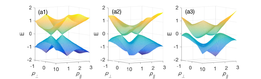
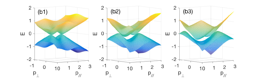
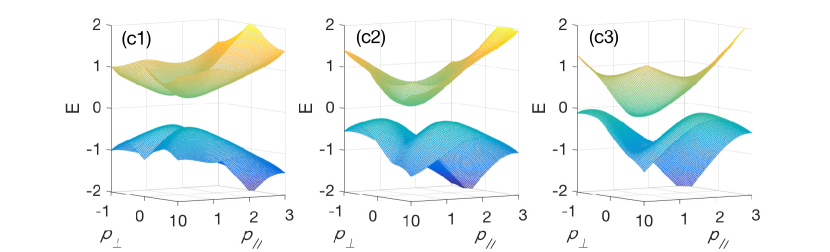
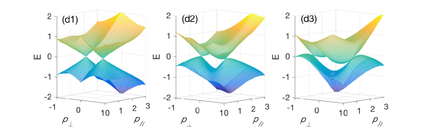
Figure 1: The energy dispersion of the two inner bands of the spectrum. Panels (a)-(d) correspond to the four cases in Eqs. (47), (49), (51), and (53) respectively. The energy offset $\delta$ is: (a1)-(d1) $\delta=0$; (a2)-(d2) $\delta=0.5$; and (a3)-(d3) $\delta=1$. The other parameters are: $p_{o}=1$, and $U\bar{m}=0.5$.

IV Example models

In this section we investigate the density wave phases in several specific lattice models which have been widely studied in the literature. The examples in Secs. IV.1 and IV.2 fall into the two types of NLs discussed in previous sections. The remainder of this section will be devoted to model beyond the simplest two-band cases.

IV.1 A model-1 loop example

A lattice model with two “model-1” loops can be described by the Hamiltonian,

$$H_{0}({\bf k}) = \left(\cos k_{x}+\cos k_{y}-m\right)\tau_{a}+\cos{k_{z}}\tau_{b}\,.$$ (55)

When $|m|<2$, the system has two NLs at $\cos{k_{x}}+\cos{k_{y}}-m=0$, in two parallel planes $k_{z}=\pm\pi/2$. They are nested by the vector $\mathbf{Q}=(0,0,\pi)$, and can be mapped to each other as

$$H_{0}({\bf k})=\tau_{a}H_{0}({\bf k}+{\bf Q})\tau_{a}\,.$$ (56)

Introducing a Hubbard interaction, the effective Hamiltonian can be written as

$$H_{eff}({\bf k}) = \left(\cos k_{x}+\cos k_{y}-m\right)t_{0}\tau_{a}+\cos{k_{z}}t_{3}\tau_{b}$$ (57)

$$+ U\bar{m}\ t_{1}\tau_{\alpha}\,.$$

We analyze first the CDW case ($\tau_{\alpha}=\tau_{0}$). Following the discussion in the previous Section, this condition corresponds to the second case in Sec. III.2, where each NL gets split into two. Indeed, from the commuting relations between different terms, we can obtain the energy dispersion as

$$E_{CDW}=\pm\sqrt{\cos^{2}{k_{z}}+\left[\cos k_{x}+\cos k_{y}-m\pm U\bar{m}\right]^{2}}\,,$$ (58)

and the split NLs are given by

$$\cos{k_{z}}=0\,,\mbox{and}\ \cos k_{x}+\cos k_{y}=m\pm U\bar{m}.$$ (59)

In the PSDW case ($\tau_{\alpha}=\tau_{3}$), different choices of $a$ and $b$ in Eq. (55) will lead to different phases of the system. In such case, the effective Hamiltonian reads

$$H_{eff}({\bf k}) = \left(\cos k_{x}+\cos k_{y}-m\right)t_{0}\tau_{a}+\cos{k_{z}}t_{3}\tau_{b}$$ (60)

$$+ U\bar{m}\ t_{1}\tau_{3},$$

and the possibilities are summarized in Table 1, and listed explicitly as follows.

a$\backslash$ b	1	2	3
1	X	loops	gapped
2	loops	X	gapped
3	metal	metal	X

Table 1: Possibilites for $\tau_{a}$, $\tau_{b}$ matrices in the loop model (55). And the resulting different outcomes of the PSDW phase.

In the case of $\tau_{a}=\tau_{3}$, the energy spectrum reads

$$E_{PSDW} = \pm\sqrt{\left(\cos k_{x}+\cos k_{y}-m\right)^{2}+\cos{k_{z}}^{2}}\pm U\bar{m}$$

with uncorrelated $\pm$ signs. This is the first case in Sec. III.2, and the ordered phase is metallic.

If $a,b\neq 3$, the spectrum reads

$$E_{PSDW}^{2} = \left(\cos k_{x}+\cos k_{y}-m\right)^{2}+\left(\cos{k_{z}}\pm U\bar{m}\right)^{2}\,,$$ (62)

where each original NL splits into two with different $k_{z}$, as in the third cases in Sec. III.2.

Finally, when $\tau_{b}=\tau_{3}$, the spectrum takes the form,

$$E^{2} = \left(\cos k_{x}+\cos k_{y}-m\right)^{2}+\cos{k_{z}}^{2}+U^{2}\bar{m}^{2}\,.$$ (63)

Thus the system is fully gapped by a nonzero $U\bar{m}$ and becomes an insulator, as in the fourth case in Sec. III.2.

IV.2 A model-2 loop example

By including $\cos{k_{z}}$ in the $\tau_{a}$ term in Eq. (55), we obtain a system with “model-2” loops, described by

$$H_{0}({\bf k})=\left(\cos k_{x}+\cos k_{y}+\cos k_{z}-m\right)\tau_{a}+\cos k_{z}\tau_{b}.$$ (64)

This system has two parallel NLs with $k_{z}=\pm\pi/2$ when $-2<m<2$. The continuous approximation for these two loops, as in Eqs. (2), satisfies $g^{\prime}_{1}=1$, and $g_{2}=g^{\prime}_{2}=-1$. Thus, the effective Hamiltonian including the Hubbard interaction is given by

$$H_{eff} = \left(\cos k_{x}+\cos k_{y}-m\right)t_{0}\tau_{a}+\cos k_{z}t_{3}\tau_{a}$$ (65)

$$+ \cos k_{z}t_{3}\tau_{b}+U\bar{m}t_{1}\tau_{\alpha}\,.$$

For the CDW case ($\tau_{\alpha}=\tau_{0}$), the spectrum reads

$$E^{2}_{CDW} = \left[\cos k_{x}+\cos k_{y}-m\pm\sqrt{U^{2}\bar{m}^{2}+\cos^{2}{k_{z}}}\right]^{2}$$ (66)

$$+\cos{k_{z}}^{2}\,,$$

thus each of the original NLs splits into two. The new NLs are given by

$$\cos{k_{z}}=0\,,\hskip 5.69046pt\cos k_{x}+\cos k_{y}=m\pm U\bar{m}.$$ (67)

In the case of PSDW ordering ($\tau_{\alpha}=\tau_{3}$), there are three possible outcomes as summarized in Table 2. In the case of $\tau_{a}=\tau_{3}$, the energy spectrum reads

$$E^{2}_{PSDW}=(\cos k_{x}+\cos k_{y}-m)^{2}+2\cos^{2}k_{z}+U^{2}\bar{m}^{2}$$

$$\pm 2\sqrt{(\cos k_{x}+\cos k_{y}-m)^{2}\left[\cos^{2}k_{z}+U^{2}\bar{m}^{2}\right]+(U\bar{m}\cos k_{z})^{2}}\,,$$

where each NL splits into two as in the second case in Sec. III.3. The condition of the NLs is the same as for the CDW case; however, as discussed in the previous section [Fig. 1(b)], these NLs have a quadratic dispersion along $k_{z}$.

a$\backslash$ b	1	2	3
1	X	loops	gapped
2	loops	X	gapped
3	loops	loops	X

Table 2: Possibilites for $\tau_{a}$, $\tau_{b}$ matrices in the loop model (64). And the resulting different outcomes of the PSDW phase.

If $\tau_{b}=\tau_{3}$ then the spectrum reads

$$E_{PSDW}^{2} = \left[\cos k_{z}\pm\sqrt{U^{2}\bar{m}^{2}+\left(\cos k_{x}+\cos k_{y}-m\right)^{2}}\right]^{2}$$ (69)

$$+ \cos^{2}k_{z}\,,$$

which is an insulating phase as in the third case in Sec. III.3.

The remaining possibility, $a,b\neq 3$, where the spectrum reads

$$E^{2}_{PSDW} = (\cos k_{x}+\cos k_{y}-m)^{2}+2\cos^{2}k_{z}+U^{2}\bar{m}^{2}$$

$$\pm 2\cos k_{z}\sqrt{(\cos k_{x}+\cos k_{y}-m)^{2}+2U^{2}\bar{m}^{2}}\,,$$

yields two NLs given by

$$\cos{k_{z}}=\pm U\bar{m}/\sqrt{2}\,,\ \cos k_{x}+\cos k_{y}=m\,.$$ (71)

This is the splitting along $k_{z}$, as in the fourth case in Sec. III.3. Finally, if we add an extra term $H_{\delta}=\delta\sin{k_{z}}\tau_{0}$ to the original Hamiltonian of Eq. (64), we can induce a energy offset $\delta$ of the two original NLs, and tilt the resulting NLs after the Hubbard interaction is introduced.

IV.3 Nested $\mathbb{Z}_{2}$ NLs

We have hitherto considered examples of two-band NLSMs, which verify our results for general two-band models. If an extra degree of freedom, say, a (pseudo)spin-1/2 subspace, is introduced, the Hilbert space is enlarged and the possibility of nodal lines carrying a $\mathbb{Z}_{2}$ monopole charge arises, which must be created in pairsZ2_loop . It is beyond the scope of this paper to extend the general analysis of Sec III. Instead, we explicitly consider a recent four-band model for $Z_{2}$ NLs Z2_loop and study density-wave order due to nesting. The model reads

$$H_{0}({\bf k}) = \sin k_{x}\tau_{0}\sigma_{1}+\sin k_{y}\tau_{2}\sigma_{2}+\sin k_{z}\tau_{0}\sigma_{3}+m\tau_{1}\sigma_{1}\,,$$

and has the spectrum

$$E_{0}^{2}({\bf k}) = \left(\sqrt{\sin^{2}k_{x}+\sin^{2}k_{y}}\pm m\right)^{2}+\sin^{2}k_{z}\,.$$ (73)

There are eight NLs, centered at momenta ${\bf k}$ with Cartesian components $k_{i}=0,\pi$ for $i=x,y,z$. We introduce a Hubbard interaction in four-dimensional space assuming that the repulsion exists between the two orbitals in subspace of $\bm{\sigma}$:

$$\hat{U} = U\sum_{{\bf r},\nu}n_{\nu 1}({\bf r})n_{\nu 2}({\bf r})=\frac{U}{2}\sum_{{\bf r}}n({\bf r})\tau_{0}\sigma_{1}n({\bf r})\,,$$ (74)

so that the remaining index $\nu=1,2$ for the two components in the subspace of $\bm{\tau}$ produces a two-fold degeneracy. In the mean-field approximation, the interaction reads (apart from unimportant constants)

$$\hat{U}_{eff} = U\bar{m}\sum_{{\bf k}}\hat{c}_{{\bf k}+{\bf Q}}^{\dagger}\tau_{0}\sigma_{z}\hat{c}_{{\bf k}}\,,$$ (75)

where we defined the PSDW as:

$$\langle n_{\nu j}({\bf r})\rangle=\frac{n}{2}+\bar{m}(-1)^{j}\cos({\bf Q}\cdot{\bf r})\,,$$ (76)

The effective 8x8 Hamiltonian has the same form as that in Eq. (26), but the anti-diagonal blocks are now written as $U\bar{m}\tau_{0}\sigma_{3}$. Two of the original $\mathbb{Z}_{2}$ loops are now coupled by the interaction. Such coupling provides an extra pseudospin-1/2 subspace, and the interaction term breaks the SU(2) symmetry in this space. As a result, the pair of NLs may either survive, shrink to point nodes, or be gapped out by the PSDW.

Depending on vector ${\bf Q}$, the effective Hamiltonian takes the form of

$$H_{eff} = \sin k_{x}t_{\alpha_{x}}\tau_{0}\sigma_{1}+\sin k_{y}t_{\alpha_{y}}\tau_{2}\sigma_{2}+\sin k_{z}t_{\alpha_{z}}\tau_{0}\sigma_{3}$$ (77)

$$+ mt_{0}\tau_{1}\sigma_{1}+U\bar{m}t_{1}\tau_{0}\sigma_{3}\,,$$

where the Pauli matrix $t_{\alpha_{i}}$ equals $t_{0}$ ($t_{3}$) for $Q_{i}=0$ ($Q_{i}=\pi$). Thus, different choices of $Q_{i}$ determine whether each term commutes or anticommutes with the interaction term $U\bar{m}t_{1}\tau_{0}\sigma_{3}$. The possibilities with different choices of ${\bf Q}$ are summarized as follows.

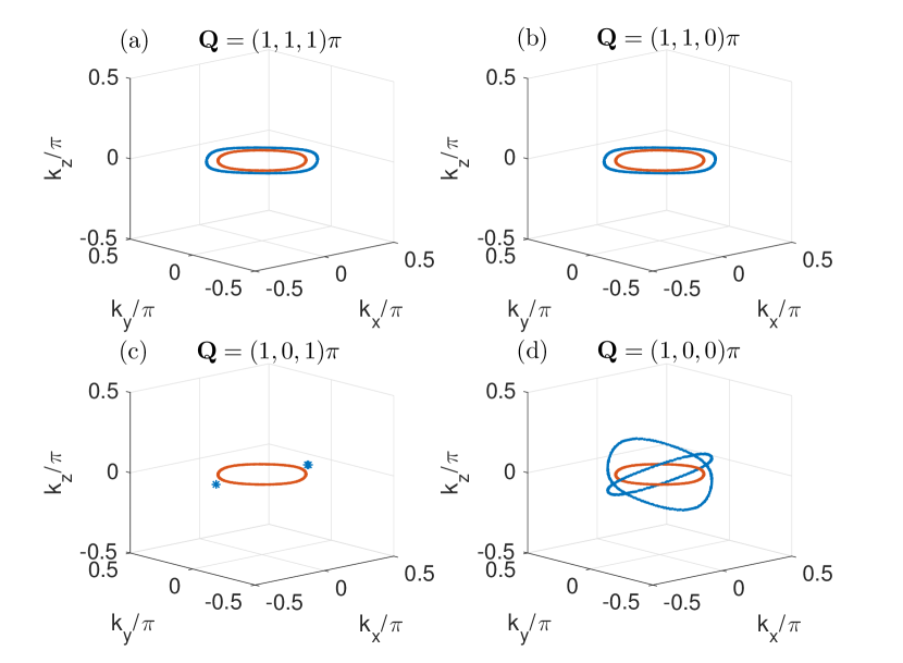
Figure 2: The effect of a PSDW on the $\mathbb{Z}_{2}$ loops for different nesting vectors ${\bf Q}$. (a) to (d) show four different cases of ${\bf Q}$ where the resulting system is still a semimetal. The red lines are the original NLs of Hamiltonian $H_{0}({\bf k})$ in Eq. (LABEL:Z2_H), whereas the blue lines and stars are the nodal lines or points in the PSDW phase. The parameters are: $m=\sqrt{2}/2$ and $U\bar{m}=0.5$. We only plot for $k_{i}\in[-\pi/2,\pi/2]$, as the graph repeats itself with a period of $\pi$.

1. ${\bf Q}=(1,1,1)\pi$:

   $$H_{eff} = \sin k_{x}t_{3}\tau_{0}\sigma_{1}+\sin k_{y}t_{3}\tau_{2}\sigma_{2}+\sin k_{z}t_{3}\tau_{0}\sigma_{3}$$ (78)

   $$+ mt_{0}\tau_{1}\sigma_{1}+U\bar{m}t_{1}\tau_{0}\sigma_{3}\,,$$

   $$E^{2} = \left(\sqrt{\sin^{2}k_{x}+\sin^{2}k_{y}}\pm\sqrt{m^{2}+U^{2}\bar{m}^{2}}\right)^{2}+\sin^{2}k_{z}\,.$$

   The spectrum is composed of four two-fold degenerate bands, and has the same NLs as the original $H_{0}$, albeit with enlarged radius [Fig. 2(a)]:

   $$k_{z}=0,\pi;\ \sqrt{\sin^{2}k_{x}+\sin^{2}k_{y}}=\sqrt{m^{2}+U^{2}\bar{m}^{2}}\,.$$ (80)

   Since the energy dispersions in Eq. (LABEL:E111) are two-fold degenerate, the NLs are four-fold degenerate.

2. ${\bf Q}=(1,1,0)\pi$:

   $$H_{eff} = \sin k_{x}t_{3}\tau_{0}\sigma_{1}+\sin k_{y}t_{3}\tau_{2}\sigma_{2}+\sin k_{z}t_{0}\tau_{0}\sigma_{3}$$ (81)

   $$+ mt_{0}\tau_{1}\sigma_{1}+U\bar{m}t_{1}\tau_{0}\sigma_{3}\,,$$

   which has the same NLs as in Eq. (80), and as shown in FIg. 2(b), despite some minor variation of the spectrum near the NLs.

3. ${\bf Q}=(1,0,1)\pi$:

   $$H_{eff} = \sin k_{x}t_{3}\tau_{0}\sigma_{1}+\sin k_{y}t_{0}\tau_{2}\sigma_{2}+\sin k_{z}t_{3}\tau_{0}\sigma_{3}$$ (82)

   $$+ mt_{0}\tau_{1}\sigma_{1}+U\bar{m}t_{1}\tau_{0}\sigma_{3}\,.$$

   The full spectrum also has the two-fold degeneracy. while the NLs are gapped in most regions, leaving only pairs of four-fold degenerate points at

   $$\sin k_{y}=\sin k_{z}=0;\ \sin k_{x}=\pm\sqrt{m^{2}+U^{2}\bar{m}^{2}}\,,$$ (83)

   as shown in Fig. 2(c).

   We note that the case ${\bf Q}=(0,1,1)\pi$ has a similar spectrum, which can be obtained from the above by performing the substitution $k_{x}\leftrightarrow k_{y}$.

4. ${\bf Q}=(1,0,0)\pi$:

   $$H_{eff} = \sin k_{x}t_{3}\tau_{0}\sigma_{1}+\sin k_{y}t_{0}\tau_{2}\sigma_{2}+\sin k_{z}t_{0}\tau_{0}\sigma_{3}$$ (84)

   $$+ mt_{0}\tau_{1}\sigma_{1}+U\bar{m}t_{1}\tau_{0}\sigma_{3}\,.$$

   Energy zeros are obtained if two conditions are simultaneously satisfied:

   $$\sum_{i=1}^{3}\sin^{2}k_{i}=U^{2}\bar{m}^{2}+m^{2}$$ (85a)

   $$m\sin k_{z}=\pm U\bar{m}\sin k_{y}\,.$$ (85b)

   Geometrically, one can think of the first condition as defining a spherical surface, for small ${\bf k}$, and the second one as two planes. The intersection between the surface and the planes yields two NLs, obtained by rotating the original loops (in the XY plane) around the $x$ axis in opposite directions. These two NLs are given by different pairs of energy bands, and thus form a nodal chain [Fig. 2(d)].

   We note that spectrum for the case ${\bf Q}=(0,1,0)\pi$ is similar to the case ${\bf Q}=(\pi,0,0)$, and differs only in the interchange $k_{x}\leftrightarrow k_{y}$. The nodal chain is obtained from the two original NLs by a rotation around the $y$ axis.

5. ${\bf Q}=(0,0,1)\pi$

   $$H_{eff} = \sin k_{x}t_{0}\tau_{0}\sigma_{1}+\sin k_{y}t_{0}\tau_{2}\sigma_{2}+\sin k_{z}t_{3}\tau_{0}\sigma_{3}$$ (86)

   $$+ mt_{0}\tau_{1}\sigma_{1}+U\bar{m}t_{1}\tau_{0}\sigma_{3}\,.$$

   In this case the system is a fully gapped insulator.

V Nested NLs in Dirac systems

In this Section we study density wave phases in four-band spinfull Hamiltonians with NLs. The spin degree of freedom allows us to distinguish two types of ordered phases: true and hidden spin density waves (SDWs). In subsection V.2 we consider NLs obtained from a perturbedBurkov ; mitschell Dirac Hamiltonian.

V.1 Spin degenerate loops

The simplest way to go from a Weyl to a Dirac loop is to introduce spin degeneracy,

$$H_{0}({\bf k})\ \rightarrow\ H_{0}({\bf k})\sigma_{0}$$ (87)

where $\sigma_{\mu}$ acts in spin space.

We assume Hubbard repulsion between two fermions having opposite spins in the same orbital (labeled by the index $j$):

$$\hat{U}=\sum_{{\bf r},j=1,2}\hat{n}_{j\uparrow}({\bf r})\hat{n}_{j\downarrow}({\bf r})\,.$$ (88)

In principle one could have ordered phases with ferromagnetic (FM) or antiferromagnetic (or SDW) configurations of the spin:

$$\langle n_{j\sigma}\rangle = \frac{1}{4}n+\bar{m}\sigma\qquad\sigma=\pm 1\,,\qquad\mbox{Stoner FM}$$ (89)

$$\langle n_{j\sigma}\rangle = \frac{1}{4}n+\bar{m}\sigma(-1)^{j}\qquad\mbox{hidden Stoner FM}$$ (90)

$$\langle n_{j\sigma}\rangle = \frac{1}{4}n+\bar{m}\sigma\cos({\bf Q}\cdot{\bf r})\qquad\mbox{true SDW}$$ (91)

$$\langle n_{j\sigma}\rangle = \frac{1}{4}n+\bar{m}\sigma(-1)^{j}\cos({\bf Q}\cdot{\bf r})\qquad\mbox{hidden SDW}$$ (92)

Because a NL’s density of states vanishes linearly with energy, the Stoner criterion precludes the FM orderings for weak interactionsroy , and they are not related to the nesting ${\bf Q}$. In the following, we shall concentrate on SDW phases. Considering the hidden SDW, Eq. (92), the effective interaction reads:

$$\hat{U}_{eff} = -U\sum_{{\bf r},j}\left[\left(\frac{n}{4}\right)^{2}-\bar{m}^{2}\cos^{2}({\bf Q}\cdot{\bf r})-\frac{n}{4}\sum_{\sigma}\hat{\psi}^{\dagger}_{j\sigma}({\bf r})\hat{\psi}_{j\sigma}({\bf r})\right]$$ (93)

$$+ U\bar{m}\sum_{{\bf r},j,j^{\prime},\sigma\sigma^{\prime}}\hat{\psi}^{\dagger}_{j\sigma}({\bf r})\ \tau^{jj^{\prime}}_{3}\sigma^{\sigma\sigma^{\prime}}_{3}\cos({\bf Q}\cdot{\bf r})\ \hat{\psi}_{j^{\prime}\sigma^{\prime}}({\bf r})\,,$$

where the field operator $\hat{\psi}_{j\sigma}({\bf r})$ now includes the spin index $\sigma$. Similarly, the field operator in momentum space $\bm{c}_{\bf k}$ now denotes $c_{{\bf k},j,\sigma}$ for all $j,\sigma$. The Hamiltonian matrix in $\left(\bm{c}^{\dagger}_{{\bf k}}\ \bm{c}^{\dagger}_{{\bf k}+{\bf Q}}\right)$ space reads (apart from unimportant constants),

$$H_{eff}({\bf k}) = \left(\begin{array}[]{cc}H_{0}({\bf k})&U\bar{m}\tau_{\alpha}\sigma_{3}\\ U\bar{m}\tau_{\alpha}\sigma_{3}&H_{0}({\bf k}+{\bf Q})\end{array}\right)\,,$$ (96)

where $\alpha=3$ describes a hidden SDW [as in Eq. (93)], and $\alpha=0$ describes a true SDW. The off-diagonal block $U\bar{m}t_{1}\tau_{3}\sigma_{3}$ has exactly the same (anti)commutation relations with the other Hamiltonian terms, as in the Weyl case of Sections III.2 and III.3 . All the criteria and spectra established for the Weyl case still hold, if one just replaces $\bar{m}\rightarrow\bar{m}\sigma_{3}$. Since this term appears as $(U\bar{m})^{2}$ in the dispersion relations, there is no spin splitting in the spectra.

We note that single antiferromagnetic NLs have been discussed in the literaturejingwang .

V.2 Two perturbed Dirac points

A nodal line Dirac semimetal can be obtained starting from a pristine 3D Dirac semimetalmitschell of the form $H_{D}({\bf k})=-\tau_{3}{\bf p}\cdot\bm{\sigma}$ and perturbing it with terms of the form $a_{\mu}\tau_{\mu}\otimes b_{\nu}\sigma_{\nu}$. Suppose, for instance,

$$H_{0}({\bf k})=-\tau_{3}{\bf p}\cdot\bm{\sigma}+\tau_{1}\bm{b}\cdot\bm{\sigma}$$ (97)

Without loss of generality assume $\bm{b}\parallel\hat{z}$. The term $p_{z}\tau_{3}\sigma_{3}$ anticommutes with the others, so:

$$E^{2}=p_{z}^{2}+\left(\sqrt{p_{x}^{2}+p_{y}^{2}}\pm b\right)^{2}\,.$$ (98)

We note that this dispersion relation is very similar to that in Eq. (73) for the $\mathbb{Z}_{2}$ loops. However, the effect of the Hubbard interaction is different, as these two systems couple the two sets of (pseudo)spin-1/2 subspace in different ways. On the other hand, Dirac points described by $H_{D}$ above do not exist alone if an additional symmetry, such as time-reversal or inversion, is present. For instance, a time-reversal symmetry (TRS) relates two Dirac points at $-\frac{1}{2}{\bf Q}$ and $+\frac{1}{2}{\bf Q}$ in such a way that:

$$\sigma_{2}H_{0}^{*}\left(\frac{{\bf Q}}{2}-{\bf k}\right)\sigma_{2}=H_{0}\left(-\frac{{\bf Q}}{2}+{\bf k}\right)\,,$$ (99)

it then follows that, for $\bm{b}=0$, $H_{0}\left(-{\bf Q}/2+{\bf k}\right)=H_{0}\left({\bf Q}/2+{\bf k}\right)=H_{D}({\bf k})$. Therefore, the two unperturbed Dirac points have the same $k\cdot p$ Hamiltonian. Including the $\tau_{1}\bm{b}\cdot\bm{\sigma}$ term, which breaks TRS, we obtain the model,

$$H_{0}\left(-\frac{{\bf Q}}{2}+{\bf k}\right) = -\tau_{3}{\bf p}\cdot\bm{\sigma}+\tau_{1}\bm{b}\cdot\bm{\sigma}\,,$$ (100a)

$$H_{0}\left(\frac{{\bf Q}}{2}+{\bf k}\right) = -\tau_{3}{\bf p}\cdot\bm{\sigma}+\tau_{1}\bm{b}\cdot\bm{\sigma}\,,$$ (100b)

and the effective Hamiltonian has equal diagonal blocks.

A different version of the above model that would preserve TRS symmetry reads:

$$H_{0}\left(-\frac{{\bf Q}}{2}+{\bf k}\right) = -\tau_{3}{\bf p}\cdot\bm{\sigma}+\tau_{1}\bm{b}\cdot\bm{\sigma}\,,$$ (101a)

$$H_{0}\left(\frac{{\bf Q}}{2}+{\bf k}\right) = -\tau_{3}{\bf p}\cdot\bm{\sigma}-\tau_{1}\bm{b}\cdot\bm{\sigma}\,.$$ (101b)

If we now consider the role of inversion symmetry ${\bf k}\rightarrow-{\bf k}$, the two Dirac points are related by

$$H_{0}\left(\frac{{\bf Q}}{2}-{\bf k}\right)=H_{0}\left(-\frac{{\bf Q}}{2}+{\bf k}\right) = -\tau_{3}{\bf p}\cdot\bm{\sigma}+\tau_{1}\bm{b}\cdot\bm{\sigma}\,,\hskip 28.45274pt$$ (102a)

$$\Rightarrow H_{0}\left(\frac{{\bf Q}}{2}+{\bf k}\right) = \tau_{3}{\bf p}\cdot\bm{\sigma}+\tau_{1}\bm{b}\cdot\bm{\sigma}\,,$$ (102b)

therefore, the two Dirac points have different $k\cdot p$ Hamiltonians.

Next we study the effects of a hidden SDW and a true SDW for these different cases, still assuming $\bm{b}\parallel\hat{z}$. For a hidden SDW, the effective Hamiltonian for the TRS breaking model in Eq. (100) is then

$$\hat{H}_{eff}=t_{0}\left[-\tau_{3}{\bf p}\cdot\bm{\sigma}+b\tau_{1}\sigma_{3}\right]+U\bar{m}t_{1}\tau_{3}\sigma_{3}\,,$$ (103)

which, by inspection produces the eight band spectrum:

$$E^{2}=\left(-p_{z}\pm U\bar{m}\right)^{2}+\left(\sqrt{p_{x}^{2}+p_{y}^{2}}\pm b\right)^{2}$$ (104)

where the $\pm$ signs are uncorrelated. This corresponds to splitting each loop along the $k_{z}$ direction.

If one considers, instead, a true SDW phase,

$$\hat{H}_{eff}=t_{0}\left[-\tau_{3}{\bf p}\cdot\bm{\sigma}+b\tau_{1}\sigma_{3}\right]+U\bar{m}t_{1}\tau_{0}\sigma_{3}\,,$$ (105)

then there are four doubly degenerate bands:

$$E^{2} = b^{2}+U^{2}\bar{m}^{2}+{\bf p}^{2}$$ (106)

$$\pm 2\sqrt{b^{2}\left(U^{2}\bar{m}^{2}+p_{x}^{2}+p_{y}^{2}\right)+U^{2}\bar{m}^{2}p_{z}^{2}}$$

with nodal lines given by $p_{z}=0\,,p_{x}^{2}+p_{y}^{2}=b^{2}-U^{2}\bar{m}^{2}$. So, the initial two loops still exist but their radius shrinks.

In the TRS model, Eq. (101), the hidden SDW phase is described by the effective Hamiltonian:

$$\hat{H}_{eff} = -t_{0}\tau_{3}{\bf p}\cdot\bm{\sigma}+bt_{3}\tau_{1}\sigma_{3}+U\bar{m}t_{1}\tau_{3}\sigma_{3}\,.$$ (107)

The spectrum is the same as in Eq. (106). So, the initial two loops still exist but their radius shrinks. And a true SDW phase is described by the effective Hamiltonian:

$$\hat{H}_{eff} = -t_{0}\tau_{3}(p_{x}\sigma_{1}+p_{y}\sigma_{2})-p_{z}t_{0}\tau_{3}\sigma_{3}+b\ t_{3}\tau_{1}\sigma_{3}$$ (108)

$$+ U\bar{m}t_{1}\tau_{0}\sigma_{3}\,,$$

which produces the spectrum with eight bands:

$$E^{2}=\left(\sqrt{p_{x}^{2}+p_{y}^{2}}\pm b\right)^{2}+\left(p_{z}\pm U\bar{m}\right)^{2}\,,$$ (109)

where the $\pm$ signs are uncorrelated. This corresponds to splitting each loop along $p_{z}=\pm U\bar{m}$.

For the case with inversion symmetry, in Eq. (102b), a hidden SDW phase is described by the effective Hamiltonian:

$$H_{eff}({\bf k})=-t_{3}\tau_{3}{\bf p}\cdot\bm{\sigma}+b\ t_{0}\tau_{1}\sigma_{3}+U\bar{m}t_{1}\tau_{3}\sigma_{3}\,,$$ (110)

which produces the eight band spectrum:

$$E^{2}=p_{z}^{2}+\left(\pm\sqrt{b^{2}+U^{2}\bar{m}^{2}}\pm\sqrt{p_{x}^{2}+p_{y}^{2}}\right)^{2}\,,$$ (111)

(uncorrelated$\pm$ signs). This corresponds to splitting each nodal line by changing its radius. A true SDW is obtained by changing $\tau_{3}\rightarrow\tau_{0}$ in the last term of Eq. (110). The resulting spectrum,

$$E^{2}=p_{z}^{2}+\left(\sqrt{p_{x}^{2}+p_{y}^{2}}\pm b\pm U\bar{m}\right)^{2}\,,$$ (112)

(with uncorrelated $\pm$ signs) also has NLs given by $p_{z}=0$, $\sqrt{p_{x}^{2}+p_{y}^{2}}=|b\pm U\bar{m}|$.

In the remaining case, where $H_{0}(-{\bf Q}/2+{\bf k})=-H_{0}({\bf Q}/2+{\bf k})$, a hidden SDW phase is described by the effective Hamiltonian:

$$H_{eff}({\bf k})=t_{3}\left[-\tau_{3}{\bf p}\cdot\bm{\sigma}+b\tau_{1}\sigma_{3}\right]+U\bar{m}t_{1}\tau_{3}\sigma_{3}\,,$$ (113)

which, by inspection produces the eight band spectrum:

$$E^{2}=p_{z}^{2}+\left(\sqrt{p_{x}^{2}+p_{y}^{2}}\pm b\pm U\bar{m}\right)^{2}\,,$$ (114)

with uncorrelated$\pm$ signs. Therefore, each loop splits in the radial direction. The true SDW is described by the effective Hamiltonian:

$$\hat{H}_{eff}=t_{3}\left[-\tau_{3}{\bf p}\cdot\bm{\sigma}+b\tau_{1}\sigma_{3}\right]+U\bar{m}t_{1}\tau_{0}\sigma_{3}\,,$$ (115)

which, by inspection produces the eight band spectrum:

$$E^{2}=p_{z}^{2}+\left(\pm\sqrt{p_{x}^{2}+p_{y}^{2}}\pm\sqrt{b^{2}+U^{2}\bar{m}^{2}}\right)^{2}\,,$$ (116)

where the $\pm$ signs are uncorrelated. Again, this corresponds to splitting each nodal loop in the radial direction.

VI Superconductivity

When considering a single Weyl NL, the pairing block of the Bogolyubov-deGennes (BdG) matrix in the particle-hole basissacramento1 ; sacramento2 ; beri , takes the form

$$\hat{\Delta}({\bf k})=\left[d_{0}({\bf k})\tau_{0}+\bm{d}({\bf k})\cdot\bm{\tau}\right]i\tau_{2}\,,$$ (117)

and fermionic statistics imposes that $\hat{\Delta}({\bf k})=\hat{\Delta}^{T}(-{\bf k})$. Close to the nodal lines the 3D momentum, ${\bf p}=\hbar{\bf k}$, can be parametrized as

$$p_{x} = (p_{0}+\tilde{p}\cos\phi)\cos\theta$$ (118a)

$$p_{y} = (p_{0}+\tilde{p}\cos\phi)\sin\theta\,,$$ (118b)

$$p_{z} = p_{\perp}=\tilde{p}\sin\phi\,,$$ (118c)

which is to be inserted in the $k\cdot p$ loops models. Here, $\theta$ is the azimuthal angle along the loop, $\tilde{p}$ is the radius of a torus involving the NL, and the angle $\phi$ wraps around the latterNandkishore1 . Note that, according to Eq. (118), momentum inversion ${\bf p}\rightarrow-{\bf p}$ is equivalent to $\theta\rightarrow\theta+\pi$ and $\phi\rightarrow-\phi$, while reflection in the loop’s plane, $p_{z}\rightarrow-p_{z}$, is equivalent to $\phi\rightarrow-\phi$.

In the semimetal case (undoped, or compensated case) the FS reduces to the NL and ${\bf p}$ reduces to the angle $\theta$ on the loop. In the doped case, any point on the torus shaped FS can be labeled by two angles, $\theta,\phi$. The functions $d_{0}({\bf k})$ and $\bm{d}({\bf k})$ describe (pseudo-spin) singlet and triplet pairing, respectively. One can expand the singlet pairing function quite generally as

$$d_{0}({\bf k})=\sum_{l_{1},l_{2}}e^{il_{1}\theta}\left[\Delta_{l_{1}l_{2}}\cos(l_{2}\phi)+\tilde{\Delta}_{l_{1}l_{2}}\sin(l_{2}\phi)\right]\,.$$ (119)

An analogous expansion can be written for $\bm{d}({\bf k})$.

If there are two nested Weyl loops, then an additional loop label must be introduced and the Pauli matrix $t_{\mu}$ operates in the two-dimensional loop space. For a two-loop system then, we write the pairing matrix as

$$\hat{\Delta}({\bf k})=\left[d_{0}({\bf k})\tau_{0}+\bm{d}({\bf k})\cdot\bm{\tau}\right]i\tau_{2}t_{\mu}\,.$$ (120)

The BdG Hamiltonian matrix in the particle-hole basis has the form

$$H({\bf k})=\left(\begin{array}[]{cc}\hat{\Xi}({\bf k})&\hat{\Delta}({\bf k})\\ \hat{\Delta}^{\dagger}({\bf k})&-\hat{\Xi}^{T}(-{\bf k})\end{array}\right)$$ (121)

with $\hat{\Xi}=diag(H_{1},H_{2})$ . The Hamiltonians $H_{1(2)}$ are the $k\cdot p$ Weyl NL models. The total Hamiltonian is then

$$\hat{H}=\frac{1}{2}\sum_{{\bf k}}{\bm{c}}^{\dagger}H({\bf k}){\bm{c}}\,,$$ (122)

where ${\bm{c}}=(\hat{\bm{c}}_{{\bf k},1},\ \hat{\bm{c}}_{{\bf k},2},\ \hat{\bm{c}}_{-{\bf k},1}^{\dagger},\ {\bm{c}}_{-{\bf k},2}^{\dagger})^{T}$. If the two NLs are centered at BZ points $\pm{\bf Q}/2$ respectively, then the inter-NL pairing is the “usual” pairing between opposite momenta, and we shall take this to be the case. If not, then the Cooper pair would have a finite quasi-momentum (a Fulde-Ferrel-Larkin-Ovchinnikov stateLOFF1 ; LOFF2 ; LOFF3 ).

The cases $\mu=0,1,3$, are different from the case $\mu=2$ regarding the parity of the functions $d_{0}({\bf k})$ and $\bm{d}({\bf k})$. In the cases $\mu=1,2$, electrons on different loops are being paired: an electron $({\bf k},1)$ is being paired with another $(-{\bf k},2)$. The cases $\mu=0,3$ describe intra-NL pairing, where the scattering of two particles from one NL into the other may be included, and $id_{0}\tau_{2}t_{3}$ would describe sign-reversed s-wave pairing, analogous to that in pnictide superconductorsBangChoi .

Inter-NL pairing with $\mu=1$ (interloop triplet pairing), requires $d_{0}$ to be even and ${\bm{d}}$ to be odd function of ${\bf k}$; if $\mu=2$ (interloop singlet), then $d_{0}$ and ${\bm{d}}$ have the opposite parities. The BdG matrix decouples into two blocks each associated with the vector spaces $(\hat{c}_{{\bf k},1},\hat{c}_{-{\bf k},2}^{\dagger})^{T}$ and $(\hat{c}_{{\bf k},2},\hat{c}_{-{\bf k},1}^{\dagger})^{T}$, respectively. Since we expect a fully gapped excitation spectrum to have higher condensation energy than a nodal spectrum, we shall examine the cases where $d_{0}$ and $\bm{d}$ are constant on the FS (in the $\mu=1$ and $\mu=2$ cases, respectively). If TRS holds, then these order parameters must also be real.

VI.1 Model-1 loops

Assuming a positive energy offset, $\delta$, the interband pairing occurs between the electronic toroidal FS from the $H_{1}-\delta$ loop, and the hole-like FS from the $H_{2}+\delta$ loop. As in previous literature, this is best done by considering projective form factorswangye ; Nandkishorepro onto the conduction or valence band. Let $U_{1(2)}$ be the unitary matrices which diagonalize $H_{1(2)}$, so that $U_{s}H_{s}U_{s}^{\dagger}=\sqrt{\left(|{\bf p}_{\parallel}|-p_{0}\right)^{2}+p_{\perp}^{2}}\ \tau_{3}\equiv\tilde{p}\tau_{3}$ for $s=1,2$. The positive and the negative branches are the conduction and valence bands, respectively. Because for model-1 loops there is always a Pauli matrix $\tau_{\beta}$ such that $H_{1}=\tau_{\beta}H_{2}\tau_{\beta}$, it then follows that $U_{2}=U_{1}\tau_{\beta}$. We can apply this same unitary transformation to the BdG matrix in Eq. (121) as:

$$\left(\begin{array}[]{cc}\Lambda&0\\ 0&\Lambda^{*}(-{\bf k})\end{array}\right)H({\bf k})\left(\begin{array}[]{cc}\Lambda^{\dagger}&0\\ 0&\Lambda^{T}(-{\bf k})\end{array}\right)$$ (127)

$$=\left(\begin{array}[]{cc}\tilde{p}\tau_{3}t_{0}-\delta\tau_{0}t_{3}&\Lambda\hat{\Delta}\Lambda^{T}(-{\bf k})\\ \Lambda^{*}(-{\bf k})\hat{\Delta}^{\dagger}\Lambda^{\dagger}&-\tilde{p}\tau_{3}t_{0}+\delta\tau_{0}t_{3}\end{array}\right)$$ (130)

where $\Lambda=diag(U_{1},U_{2})$. The off-diagonal pairing block is then $\Lambda({\bf k})\hat{\Delta}({\bf k})\Lambda^{T}(-{\bf k})$.

For $\delta>0$, only the pairing between the conduction band of $H_{1}$ and the valence band of $H_{2}$ is considered. From the BdG matrix in Eq. (130) we obtain the submatrix operating in this two-fold subspace as:

$$H^{FS}=\left(\begin{array}[]{cc}\tilde{p}-\delta&\Delta_{FS}({\bf k})\\ \Delta_{FS}^{*}({\bf k})&\tilde{p}-\delta\end{array}\right)$$ (133)

where $\Delta_{FS}({\bf k})$ is the pairing function on the FS which, from Eq. (130) and for $\mu=1$ reads:

$$\Delta_{FS}({\bf k})=\left[U_{1}({\bf k})\left(d_{0}+{\bm{d}}\cdot{\bm{\tau}}\right)i\tau_{2}U_{2}^{T}(-{\bf k})\right]_{12}$$ (134)

It is then clear from Eq. (133) that the spectrum is $E=\tilde{p}-\delta\pm|\Delta_{FS}({\bf k})|$, and is gapless. At finite doping, no gapped state is to be expected from FS interloop pairing between non-degenerate model-1 Weyl loops.

The situation is different for the degenerate ($\delta=0$) case, however, where the FS is composed of two nodal lines. From Eq. (130) and $t_{\mu}=t_{1}$ we obtain a BdG matrix restricted to the subspace $\left(U_{1}({\bf k})\hat{\bm{c}}_{{\bf k},1}\,,U_{2}^{*}(-{\bf k})\hat{\bm{c}}_{-{\bf k},2}^{\dagger}\right)$, as

$$H_{12}^{\prime}=\left(\begin{array}[]{cc}\tilde{p}\tau_{3}&U_{1}(d_{0}+{\bm{d}}\cdot{\bm{\tau}})i\tau_{2}U_{2}^{T}\\ -iU_{2}^{*}\tau_{2}(d_{0}+{\bm{d}}\cdot{\bm{\tau}})U_{1}^{\dagger}&-\tilde{p}\tau_{3}\end{array}\right)$$ (137)

For the sake of definiteness we consider the NL models with $\tau_{a}=\tau_{1},\tau_{b}=\tau_{2}$, so that

$$H_{1}(\phi) = \tilde{p}\left(\cos\phi\tau_{1}+\sin\phi\tau_{2}\right)\,,$$ (138)

$$U_{1}({\bf k}) = \frac{1}{\sqrt{2}}\left(\begin{array}[]{cc}1&e^{-i\phi}\\ -1&e^{-i\phi}\end{array}\right)\,.\$$ (141)

We note that all the other $(\tau_{a},\tau_{b})$ cases can be related to this through a suitable rotation in pseudo-spin space. From Eq. (141), one can see that $U_{1}^{\dagger}({\bf k})=U_{1}^{T}(-{\bf k})$. Interloop pairing is described by the off-diagonal block in Eq (137):

$$U_{1}({\bf k})\left(d_{0}+{\bm{d}}\cdot{\bm{\tau}}\right)i\tau_{2}\tau_{\beta}^{T}U_{1}^{T}(-{\bf k})=$$ (144)

$$= \left(\begin{array}[]{cc}id_{0}\sin\phi+id_{2}+d_{3}\cos\phi&d_{0}\cos\phi+d_{1}+id_{3}\sin\phi\\ -d_{0}\cos\phi+d_{1}-id_{3}\sin\phi&-id_{0}\sin\phi+id_{2}-d_{3}\cos\phi\end{array}\right)\,,$$

$$= \left(\begin{array}[]{cc}d_{3}+id_{2}\cos\phi-id_{1}\sin\phi&-d_{0}-d_{1}\cos\phi-d_{2}\sin\phi\\ -d_{0}+d_{1}\cos\phi+d_{2}\sin\phi&d_{3}-id_{2}\cos\phi+id_{1}\sin\phi\end{array}\right)\,,$$ (147)

$$= \left(\begin{array}[]{cc}-id_{0}-id_{1}\cos\phi-id_{2}\sin\phi&d_{1}\sin\phi-d_{2}\cos\phi+id_{3}\\ -d_{1}\sin\phi+d_{2}\cos\phi+id_{3}&-id_{0}+id_{1}\cos\phi+id_{2}\sin\phi\end{array}\right)\,,$$ (150)

$$= \left(\begin{array}[]{cc}-d_{0}\cos\phi-d_{1}-id_{3}\sin\phi&-id_{0}\sin\phi-id_{2}-d_{3}\cos\phi\\ id_{0}\sin\phi-id_{2}+d_{3}\cos\phi&d_{0}\cos\phi-d_{1}+id_{3}\sin\phi\end{array}\right)\,,$$ (153)

for the cases $\beta=0,1,2,3$, respectively. Note that for the case $t_{\mu}=t_{2}$, we simply have to multiply both sides of Eq. (LABEL:udelu) by $-i$.

For $\mu=1$ a fully gapped FS can only happen for constant $d_{0}$ because $\bm{d}$ is an odd function and must have nodes on the NLs. In this case, only for $\beta=2$ a gapped spectrum is obtained: $E^{2}=\tilde{p}^{2}+d_{0}^{2}$.

For $\mu=2$ (interloop singlet) and constant real $\bm{d}$ there are more possibilities. If $\beta=0$ a fully gapped spectrum $E^{2}=\tilde{p}^{2}+d_{2}^{2}$; if $\beta=1$ a fully gapped spectrum $E^{2}=\tilde{p}^{2}+d_{3}^{2}$; for $\beta=3$ the fully gapped spectrum $E^{2}=\tilde{p}^{2}+d_{1}^{2}$. Gapped spectra result from intraband pairing. Interband pairing leads to nodal spectra for the same reason as in the $\delta>0$ case.

VI.2 Model-2 loops

In a model-2 loop we replace Eqs. (138)-(141) with

$$H_{1}(\phi) = \tilde{p}\left[(\cos\phi+\sin\phi)\tau_{1}+\sin\phi\tau_{2}\right]\,,$$ (155)

$$U_{1}({\bf k}) = \frac{1}{\sqrt{2}}\left(\begin{array}[]{cc}e^{i\omega}&1\\ e^{-i\omega}&-1\end{array}\right)\,,$$ (158)

where $\omega=arg(e^{i\phi}+\sin\phi)$. If $H_{1}=\tau_{\beta}H_{2}\tau_{\beta}$, then the conclusions are the same as for model-1 loops, with the replacement $\tilde{p}\rightarrow\tilde{p}|e^{i\phi}+\sin\phi|$.

We now consider the case where the two loops are related through the reflection operation in Eq. (42). Because the reflection implies $\phi\rightarrow-\phi$, the energy dispersions are different for $H_{1}$ and $H_{2}$. In the non-degenerate case ($\delta>0$), $H^{FS}$ now takes the form

$$H^{FS}=\left(\begin{array}[]{cc}\tilde{p}|e^{i\phi}+\sin\phi|-\delta&\Delta_{FS}({\bf k})\\ \Delta_{FS}^{*}({\bf k})&\tilde{p}|e^{i\phi}-\sin\phi|-\delta\end{array}\right)$$ (161)

and the resulting spectrum allows gapless excitations, as was the case for model-1 loops.

In the degenerate case, we find it more convenient not to perform the rotation in Eq. (130), and diagonalize the original BdG matrix restricted to the subspace $\left(\hat{\bm{c}}_{{\bf k},1}\,,\hat{\bm{c}}_{-{\bf k},2}^{\dagger}\right)$, instead. In this subspace, the two diagonal blocks of the BdG matrix, which follow from Eq. (121), are $H_{1}(\phi)$ and

$$-H_{2}^{T}(-\phi) = -\tau_{\beta}H_{1}^{T}(\phi)\tau_{\beta}\,,$$ (162)

which follows from (155) and the reflection operation that relates both loops: $H_{2}(\phi)=\tau_{\beta}H_{1}(-\phi)\tau_{\beta}$. For $t_{\mu}=t_{1}$ (interloop triplet) the BdG reads:

$$H_{12}^{\prime}=\left(\begin{array}[]{cc}H_{1}\phi)&(d_{0}+{\bm{d}}\cdot{\bm{\tau}})i\tau_{2}\\ -i\tau_{2}(d_{0}+{\bm{d}}\cdot{\bm{\tau}})&-\tau_{\beta}H_{1}^{T}(\phi)\tau_{\beta}\end{array}\right)$$ (165)

We identify the TRS cases where the excitation spectrum is fully gapped. For constant $d_{0}$ and ${\bm{d}}=0$, the gapped spectra are obtained for $\beta=1$ and $\beta=3$, respectively:

$$\beta=1:E^{2} = d_{0}^{2}+{\tilde{p}}^{2}\sin^{2}\phi+\left(d_{0}\pm\tilde{p}|\sin\phi+\cos\phi|\right)^{2}\,,$$

$$\beta=3:E^{2} = d_{0}^{2}+{\tilde{p}}^{2}\left[\sin^{2}\phi+(\sin\phi+\cos\phi)^{2}\right]\,.$$ (167)

In the case of interloop singlet $t_{\mu}=t_{2}$, we consider $d_{0}=0$ and constant $\bm{d}$. Gapped spectra exist for: $\beta=0$ and nonzero $d_{3}$; $\beta=1$ and nonzero $d_{2}$; $\beta=2$ and nonzero $d_{1}$. All these cases have similar spectra:

$$\beta=0:E^{2} = d_{3}^{2}+{\tilde{p}}^{2}\left[\sin^{2}\phi+(\sin\phi+\cos\phi)^{2}\right]\,,\ \$$ (168a)

$$\beta=1:E^{2} = d_{2}^{2}+{\tilde{p}}^{2}\left[\sin^{2}\phi+(\sin\phi+\cos\phi)^{2}\right]\,,\ \$$ (168b)

$$\beta=2:E^{2} = d_{1}^{2}+{\tilde{p}}^{2}\left[\sin^{2}\phi+(\sin\phi+\cos\phi)^{2}\right]\,.\ \$$ (168c)

VI.3 Pairing between Dirac loops

Including the spin degree of freedom, we may discuss the pairing between spin degenerate loops $H_{1}\otimes\sigma_{0}$ and $H_{2}\otimes\sigma_{0}$ described by the BdG matrix:

$$H_{12,s}^{\prime}=\left(\begin{array}[]{cc}H_{1}\otimes\sigma_{0}&(d_{0}+{\bm{d}}\cdot{\bm{\tau}})i\tau_{2}(t_{\mu})_{12}\sigma_{s}\\ -i\sigma_{s}\tau_{2}(d_{0}+{\bm{d}}\cdot{\bm{\tau}})(t_{\mu})_{21}&-H_{2}^{T}\otimes\sigma_{0}\end{array}\right)$$ (171)

Whatever the choice for $s=1,2,3$, $H_{12,s}^{\prime}$ decouples in subblocks for which the results obtained above for Weyl systems can be applied. The (anti)symmetric property of the matrices $t_{\mu}$, $\sigma_{s}$ will determine whether the functions $d_{0}$,$\bm{d}$ should be odd of even: if for instance, $s=1,3$ then the parity of $d_{0}$,$\bm{d}$ is as in the Weyl case; if, however, $s=2$ (spin singlet), then the parities should be reversed.

VII Summary and Conclusions

We have described broken symmetry phases of nested Weyl and Dirac NLs that are induced by a short range interaction. We made a systematic analysis for two-band Hamiltonians with PT symmetry, where the two nested Weyl NLs can be mapped onto each other through a rotation or reflection operator. Charge and (pseudo)spin density waves always lower the energy and the broken symmetry phase can be metallic, semimetallic or insulating, depending on the operator that maps the the initial NLs onto each other, and on whether they enjoy a local reflection symmetry in the loop plane. This outcome does not depend on whether the initial system is semimetallic or metallic (when the initial FS is composed of two toroidal FSs, one hole- and one electron-like). If the initial system is semimetallic, spontaneous symmetry breaking requires a finite interaction which is attractive for CDWs and repulsive for PSDWs.

We have also studied specific four-band models, including the $\mathbb{Z}_{2}$ NLs, spin degenerate Dirac systems, and NL’s derived from perturbed spinful Dirac nodal points. The PSDW phases from $\mathbb{Z}_{2}$ NLs include nodal point and nodal chain semimetals.

Fully gapped superconducting phases from electron pairing in different NLs (interloop pairing), with TRS, have been found. They include all possibilities of triplet and singlet pairing in loop space and spin space.

There has recently been an intensive search for topological semimetal materials. Given that point nodes tend to appear in pairs for symmetry reasons, it is conceivable that suitable engineering can produce double NLs. Indeed, a recent proposal for realizing point nodes (Dirac or Weyl), and pairs of NLs by strain engineering in SnTe and GeTe is relevant hereLauOrtix . Another recent proposal concerns layered ferromagnetic rare-earth-metal monohalides LnX (Ln=La, Gd; X=Cl, Br) and a pair of mirror-symmetry protected nodal lines in LaX and GdXNie . Also, splitting of Dirac rings into pairs of Weyl rings by spin-orbit interaction in InNbS₂ has been proposedDu . Two groups of Dirac nodal rings have been experimentally detectedLou in ZrB₂. However, the detection of pairs of NLs at the Fermi level is presently still lacking.

We have not addressed the competition between different orderings or interactions, but such an extension of our work might be relevant to real materials. We have also neglected the effect of the long-ranged tail of the Coulomb interaction which could be present if the starting system is a NL semimetal with the screening radius diverging near the Fermi level. In this respect, the study in Ref[roy ] for a single NL suggests that the critical interaction strength for orderings where a fully gapped spectrum arises could be lowered.

Ordered phasesgruner , such as orbital and/or spin density waves, can be detected through neutron scattering, or resonant soft x-ray scatteringxray . The band structure itself may be studied with angle-resolved photoemission spectroscopy.

Appendix A Energy spectrum for Hamiltonian (32)

Taking $\alpha=0$, (CDW case), for instance, and $(a,b)=(1,2)$, the rotated effective Hamiltonian in Eq. (32) then reads:

$$AH_{eff}({\bf k})A^{\dagger}=\left(p_{\parallel}-p_{o}\right)t_{0}\tau_{1}+p_{\perp}t_{0}\tau_{2}+U\bar{m}\ t_{1}\tau_{\beta}-\delta\ t_{3}\tau_{0}\,.$$ (173)

We perform a suitable rotation on the Hamiltonian $AH_{eff}A^{\dagger}$ in Eq. (173) so that its energy spectrum can be written down by inspecting the (anti)commutation relations among its terms. If $\beta=1$ or 2, we introduce a SU(2) rotation in $t_{\mu}$ space so that in the end, only the matrix $t_{3}$ appears. The required rotation is

$$W=\cos\frac{\theta}{2}-it_{2}\tau_{\beta}\sin\frac{\theta}{2}\,,$$ (174)

with the rotation angle $\theta$ given by

$$\sin\theta = \frac{U\bar{m}}{\sqrt{U^{2}\bar{m}^{2}+\delta^{2}}}\,,$$ (175a)

$$\cos\theta = \frac{\delta}{\sqrt{U^{2}\bar{m}^{2}+\delta^{2}}}\,,$$ (175b)

so that the rotated Hamiltonian for $\beta=1$ reads

$$WAH_{eff}A^{\dagger}W^{\dagger} = \left(p_{\parallel}-p_{o}\right)\tau_{1}+p_{\perp}\cos\theta\ \tau_{2}$$ (176)

$$+ p_{\perp}\sin\theta\ t_{2}\tau_{3}$$

$$- \sqrt{U^{2}\bar{m}^{2}+\delta^{2}}\ t_{3}\,,$$

and the energy spectrum obeys

$$E^{2} = \left[\sqrt{\left(p_{\parallel}-p_{o}\right)^{2}+p_{\perp}^{2}\cos^{2}\theta}\pm\sqrt{U^{2}\bar{m}^{2}+\delta^{2}}\right]^{2}$$ (177)

$$+ p_{\perp}^{2}\sin^{2}\theta\,,$$

which is equivalent to Eq. (37).

For $\beta=2$ we have

$$WAH_{eff}A^{\dagger}W^{\dagger} = \left(p_{\parallel}-p_{o}\right)\cos\theta\ \tau_{1}+p_{\perp}\tau_{2}$$ (178)

$$- \left(p_{\parallel}-p_{o}\right)\sin\theta\ t_{2}\tau_{3}$$

$$- \sqrt{U^{2}\bar{m}^{2}+\delta^{2}}\ t_{3}\,,$$

and the energy spectrum obeys

$$E^{2} = \left[\sqrt{\left(p_{\parallel}-p_{o}\right)^{2}\cos^{2}\theta+p_{\perp}^{2}}\pm\sqrt{U^{2}\bar{m}^{2}+\delta^{2}}\right]^{2}$$ (179)

$$+ \left(p_{\parallel}-p_{o}\right)^{2}\sin^{2}\theta\,,$$

which is equivalent to Eq. (38).

In the case $\beta=3$, it is preferable to perform a SU(2) rotation in $\tau$ space in order to eliminate one of the Pauli matrices $\tau$. To this aim, we introduce

$$R_{c}=\cos\frac{\theta}{2}-i\tau_{3}\sin\frac{\theta}{2}\,,$$ (180)

with

$$\sin\theta = \frac{p_{\parallel}-p_{o}}{\sqrt{\left(p_{\parallel}-p_{o}\right)^{2}+\delta^{2}}}\,,$$ (181a)

$$\cos\theta = \frac{p_{\perp}}{\sqrt{\left(p_{\parallel}-p_{o}\right)^{2}+\delta^{2}}}\,,$$ (181b)

so that the rotation of the Hamiltonian now works out as,

$$R_{c}AH_{eff}A^{\dagger}R_{c}^{\dagger} = {\sqrt{\left(p_{\parallel}-p_{o}\right)^{2}+\delta^{2}}}\ \tau_{2}+U\bar{m}\ t_{1}\tau_{3}-\delta\ t_{3}\,.$$

More generally, if the product $\tau_{\alpha}\tau_{\beta}=i\epsilon_{\alpha\beta j}\tau_{j}$, then the above results for the energy still hold, because the appearance of the factor $i$ in the $U\bar{m}$ term would lead to the replacement $t_{1}\rightarrow t_{2}$ in (173), which does not change the (anti)commutation relations among the Hamiltonian terms.

Appendix B Mean field treatment of PSDW/CDW

Given the order parameter for a PSDW, $\langle n_{s}({\bf r})\rangle=\frac{1}{2}n+\bar{m}(-1)^{s}\cos({{\bf Q}}\cdot{\bf r})$, one may transform to Fourier space as

$$\langle n_{s}({\bf r})\rangle=\frac{1}{N}\sum_{{\bf q}}\langle c_{{\bf q}s}^{\dagger}c_{{\bf q}s}\rangle+e^{i{\bf Q}\cdot{\bf r}}\langle c_{{\bf q}s}^{\dagger}c_{{\bf q}+{\bf Q}s}\rangle+e^{-i{\bf Q}\cdot{\bf r}}\langle c_{{\bf q}+{\bf Q}s}^{\dagger}c_{{\bf q}s}\rangle\,.$$

Using $\hat{\psi}_{s}({\bf r})=\sum_{{\bf q}}e^{i{\bf q}\cdot{\bf r}}c_{{\bf q}s}/\sqrt{N}$, where $N$ is the number of momentum values in the summation, we see that the above $\langle n_{s}({\bf r})\rangle$ is obtained if

$$\frac{1}{N}\sum_{{\bf q}}\langle c_{{\bf q}s}^{\dagger}c_{{\bf q}s}\rangle = \frac{1}{2}n\,,$$ (184)

$$\frac{1}{N}\sum_{{\bf q}}\langle c_{{\bf q}+{\bf Q}s}^{\dagger}c_{{\bf q}s}\rangle=\frac{1}{N}\sum_{{\bf q}}\langle c_{{\bf q}s}^{\dagger}c_{{\bf q}+{\bf Q}s}\rangle = \frac{1}{2}\bar{m}(-1)^{s}\,,$$ (185)

for $\alpha=3$ (PSDW). If $\alpha=0$ (CDW) then the factor $(-1)^{s}$ should be omitted. The Hamiltonian is given by

$$\hat{H}_{eff}=\frac{1}{2}\sum_{{\bf k}}(\hat{\bm{c}}_{{\bf k}}^{\dagger}\hat{\bm{c}}_{{\bf k}+{\bf Q}}^{\dagger})H_{eff}({\bf k})\left(\begin{array}[]{c}\hat{\bm{c}}_{{\bf k}}\\ \hat{\bm{c}}_{{\bf k}+{\bf Q}}\end{array}\right)$$ (188)

where $\hat{\bm{c}}_{{\bf k}}=(\hat{c}_{{\bf k},1}\hat{c}_{{\bf k},2})$. We assume that $H_{eff}({\bf k})$ is diagonalized by a unitary matrix, $S$, so that $SH_{eff}({\bf k})S^{\dagger}$ is the diagonal matrix composed of the eigenenergies. Then, the operators $\hat{\bm{\gamma}}$ which destroy the elementary excitations are given by

$$\hat{\bm{\gamma}}=S\left(\begin{array}[]{c}\hat{\bm{c}}_{{\bf k}}\\ \hat{\bm{c}}_{{\bf k}+{\bf Q}}\end{array}\right)\,.$$ (191)

Following Eq. (185) we can see that

$$\frac{1}{N}\sum_{{\bf k}}\langle(\hat{\bm{c}}_{{\bf k}}^{\dagger}\hat{\bm{c}}_{{\bf k}+{\bf Q}}^{\dagger})\left(\begin{array}[]{cc}0&\tau_{\alpha}\\ \tau_{\alpha}&0\end{array}\right)\left(\begin{array}[]{c}\hat{\bm{c}}_{{\bf k}}\\ \hat{\bm{c}}_{{\bf k}+{\bf Q}}\end{array}\right)\rangle=\mp 2\bar{m}\left\{\begin{array}[]{c}\alpha=3\\ \alpha=0\end{array}\right.$$ (198)

or, in the eigenbasis using (191),

$$\frac{1}{N}\sum_{{\bf k}}\langle\hat{\bm{\gamma}}^{\dagger}S\left(\begin{array}[]{cc}0&\tau_{\alpha}\\ \tau_{\alpha}&0\end{array}\right)S^{\dagger}\hat{\bm{\gamma}}\rangle\ =\mp 2\bar{m}\left\{\begin{array}[]{c}\alpha=3\\ \alpha=0\end{array}\right.$$ (203)

$$= \frac{1}{N}\sum_{{\bf k}}\sum_{j}\left[S\left(\begin{array}[]{cc}0&\tau_{\alpha}\\ \tau_{\alpha}&0\end{array}\right)S^{\dagger}\right]_{jj}f(E_{j}({\bf k}))\,,$$ (206)

where $f(x)=1/(1+e^{x/T})$ denotes the Fermi-Dirac distribution function, and $j=1,...,4$ denotes a band index. The energy dispersions, $E_{j}({\bf k})$, are given in the main text. However, it is more convenient to work with the transformed Hamiltonian $AH_{eff}A^{\dagger}$ as in the main text, which implies that all operators are similarly rotated and $S\rightarrow SA^{\dagger}$ above. Then, Eq. (206) can be written in the form,

$$\frac{1}{N}\sum_{{\bf k}}\sum_{j}\left[SA^{\dagger}\left(\begin{array}[]{cc}0&\tau_{\alpha}\tau_{\beta}\\ \tau_{\beta}\tau_{\alpha}&0\end{array}\right)AS^{\dagger}\right]_{jj}f(E_{j}({\bf k}))$$ (209)

$$= \mp 2\bar{m}\left\{\begin{array}[]{c}\alpha=3\\ \alpha=0\end{array}\right.\,.$$ (212)

Appendix C Critical interaction $U_{cr}$ for degenerate NLs

We consider a circular nodal line and use the momentum parametrization in Eq. (118).

We linearize the theory in a toroidal region surrounding the NL up to a momentum cutoff: $0<\tilde{p}<\tilde{p}_{c}$, $0<\theta,\phi<2\pi$. The volume element is $d^{3}p=(p_{0}+\tilde{p}\cos\phi)\tilde{p}\cdot d\tilde{p}d\theta d\phi$. The number of ${\bf k}$ terms in the toroidal region around the NL is then given by

$$N=\frac{1}{(2\pi\hbar)^{3}}\int d^{3}p = \frac{p_{0}\tilde{p}_{c}^{2}}{4\pi\hbar^{3}}\,.$$ (214)

In order to simplify the calculations, it is assumed that the dispersion relation has the same velocity, $v$, in the NL plane and perpendicular to it. Then, using $p_{\parallel}-p_{0}=\tilde{p}\cos\phi$, the model-1 NL Eq. (1.a) reads

$$H_{0}({\bf k})=v\tilde{p}\left(\cos\phi\tau_{1}+\sin\phi\tau_{2}\right)\,,$$ (215)

where $v=v_{1}=v_{2}$ and we shall take $\delta=0$. As before, we proceed considering the velocity $v=1$ and but shall restore it in the final result for $U_{cr}$. In the cases where $\tau_{\alpha}\tau_{\beta}\propto\tau_{1}$ and $\tau_{\alpha}\tau_{\beta}\propto\tau_{2}$ the ordered phases are semimetalic and yield similar mean field equations. In the case where $\tau_{\alpha}\tau_{\beta}\propto\tau_{2}$, for instance, the negative energy bands are

$$E_{1(2)} = -\sqrt{\tilde{p}^{2}\pm 2\tilde{p}U\bar{m}\sin\phi+U^{2}\bar{m}^{2}}$$ (216)

and the l.h.s. of Eq. (LABEL:APMFeq) takes the form,

$$\frac{1}{N}\sum_{{\bf k}}\sum_{j}\left[SA^{\dagger}\left(\begin{array}[]{cc}0&\tau_{\alpha}\tau_{\beta}\\ \tau_{\beta}\tau_{\alpha}&0\end{array}\right)AS^{\dagger}\right]_{jj}f(E_{j}({\bf k}))$$ (219)

$$= \frac{1}{N}\ \int\frac{2(\tilde{p}\sin\phi-U\bar{m})(p_{0}+\tilde{p}\cos\phi)d^{3}p}{(2\pi\hbar)^{3}\sqrt{\tilde{p}^{2}-2\tilde{p}U\bar{m}\sin\phi+U^{2}\bar{m}^{2}}}\,.$$ (220)

In the limit $U\bar{m}\rightarrow 0$ one can Taylor expand the integrand to first order. The mean field equations (LABEL:APMFeq) yield

$$\frac{p_{0}\tilde{p}_{c}}{4\pi N\hbar^{3}}=\pm\frac{1}{U_{cr}}\Longrightarrow\ U_{cr}=\pm v\tilde{p}_{c}\left\{\begin{array}[]{c}\alpha=3\\ \alpha=0\end{array}\right.\,,$$ (223)

where we used (214) and the velocity $v$ has been restored. The finiteness of $U_{cr}$ stems from the linear form of the density of states near the Fermi level. The case where $\tau_{\alpha}\tau_{\beta}\propto\tau_{c\neq a,b}$, where the PSDW phase is insulating, yields a similar result modified by a prefactor of $1/2$: $U_{cr}=\pm v\tilde{p}_{c}/2$. This is valid also for the case $\tau_{\alpha}\tau_{\beta}=1$, where the density wave phase is metallic. We see then that the CDW phase requires an attractive interaction.

References

- (1) K. Mullen, B. Uchoa, and D. T. Glatzhofer, Phys. Rev. Lett. 115, 026403 (2015).
- (2) J. L. Lu, X. Y. Li, S. Q. Yang, J. X. Cao, X. G. Gong, and H. J. Xiang, Chin. Phys. Lett. 34, 057302 (2017).
- (3) A. A. Burkov, M. D. Hook, and L. Balents, Phys. Rev. B 84, 235126 (2011).
- (4) S. A. Yang, H. Pan, and F. Zhang, Phys. Rev. Lett. 113, 046401 (2014).
- (5) Y. Chen, Y. Xie, S. A. Yang, H. Pan, F. Zhang, M. L. Cohen, and S. Zhang, Nano Letters 15, 6974 (2015).
- (6) H. Weng, Y. Liang, Q. Xu, R. Yu, Z. Fang, X. Dai, and Y. Kawazoe, Phys. Rev. B 92, 045108 (2015).
- (7) D.-W. Zhang, Y. X. Zhao, R.-B. Liu, Z.-Y. Xue, S.-L. Zhu, and Z. D. Wang, Phys. Rev. A 93, 043617 (2016).
- (8) C. Zhong, Y. Chen, Z.-M. Yu, Y. Xie, H. Wang, S. A. Yang, and S. Zhang, Nat. Comm. 8, 15641 (2017).
- (9) M. Ezawa, Phys. Rev. B 96, 041202 (2017).
- (10) Z. Yan, R. Bi, H. Shen, L. Lu, S.-C. Zhang, and Z. Wang, Phys. Rev. B 96, 041103 (2017).
- (11) W. Chen, H.-Z. Lu, and J.-M. Hou, Phys. Rev. B 96, 041102 (2017).
- (12) Y. Zhou, F. Xiong, X. Wan, and J. An, Phys. Rev. B 97, 155140 (2018).
- (13) L. Li, C. H. Lee, and J. Gong, Phys. Rev. Lett. 121, 036401 (2018).
- (14) Y. Kim, B. J. Wieder, C. L. Kane, and A. M. Rappe, Phys. Rev. Lett. 115, 036806 (2015).
- (15) R. Yu, H. Weng, Z. Fang, X. Dai, and X. Hu, Phys. Rev. Lett. 115, 036807 (2015).
- (16) A. Narayan, Phys. Rev. B 94, 041409 (2016).
- (17) K. Taguchi, D.-H. Xu, A. Yamakage, and K. T. Law, Phys. Rev. B 94, 155206 (2016).
- (18) C.-K. Chan, Y.-T. Oh, J. H. Han, and P. A. Lee, Phys. Rev. B 94, 121106 (2016).
- (19) X.-X. Zhang, T. T. Ong, and N. Nagaosa, Phys. Rev. B 94, 235137 (2016).
- (20) Z. Yan and Z. Wang, Phys. Rev. Lett. 117, 087402 (2016).
- (21) Z. Yan and Z. Wang, Phys. Rev. B 96, 041206 (2017).
- (22) L. Li, C. Yin, S. Chen, and M. A. N. Araújo, Phys. Rev. B 95, 121107 (2017).
- (23) L. Li, H. H. Yap, M. A. N. Araújo, and J. Gong, Phys. Rev. B 96, 235424 (2017).
- (24) S. Sur and R. Nandkishore, New J. Phys. 18 115006 (2016).
- (25) R. Nandkishore, Phys. Rev B 93, 020506 (2016).
- (26) H. Shapourian, Y. Wang, and S. Ryu, Phys. Rev B 97, 094508 (2018).
- (27) B. Roy, Phys. Rev B 96, 041113 (2017).
- (28) Y. Wang and P. Ye Phys. Rev B 94, 075115 (2016).
- (29) P.-Y. Chang, and C.-H. Yee, Phys. Rev. B 96, 081114 (2017).
- (30) C. Fang, Y. Chen, H.-Y. Kee, and L. Fu, Phys. Rev. B 92, 081201 (2015).
- (31) G. Bian et. at., Phys. Rev B 93, 121113 (2016).
- (32) George Grüner, Density waves in solids (Addison-Wesley Publishing Company, 1994).
- (33) A. K. Mitchell and L. Fritz, Phys. Rev B 93, 035137 (2016).
- (34) J. Wang, Phys. Rev B 96, 081107 (2017).
- (35) P. D. Sacramento, M. A. N. Araújo, and E. V. Castro, Europhys. Lett. 105, 37011 (2014).
- (36) P. D. Sacramento, M. A. N. Araújo, V. R. Vieira, V. K. Dugaev, and J. Barnaś, Phys. Rev B 85, 014518 (2012).
- (37) B. Béri, Phys. Rev B 81, 134515 (2010).
- (38) Y. Bang, and H.-Y. Choi, Phys. Rev B 78, 134523 (2008).
- (39) P. Fulde, and A. Ferrel, Phys. Rev. 135, A550 (1964).
- (40) A. I. Larkin, and Y. N. Ovchinnikov, Sov. Phys. JETP-USSR 20, 762 (1965).
- (41) H. Shimahara, Phys. Rev B 50, 12760 (1994).
- (42) Y. Wang, and R. M. Nandkishore, Phys. Rev. 95, 060506 (2017).
- (43) A. Lau, and C. Ortix, arXiv:1804.09574.
- (44) S. Nie, H. Weng, and F. B. Prinz, arXiv:1803.08486.
- (45) Y. Du, X. Bo, D. Wang, E.-J. Kan, C.-G. Duan, S. Y. Savrasov, and X. Wan, Phys. Rev. B 96, 235152 (2017).
- (46) R. Lou, P. Guo, M. Li, Q. Wang, Z. Liu, S. Sun, C. Li, X. Wu, Z. Wang, Z. Sun, D. Shen, Y. Huang, K. Liu, Z-Y Lu, H. Lei, H. Ding, and S. Wang, npj Quantum Materials 3, 43 (2018).
- (47) B. Pan, H. Jang, J.-S. Lee, R. Sutarto, F. He, J. F. Zeng, Y. Liu, X. Zhang, Y. Feng, Y. Hao, J. Zhao, H. C. Xu, Z. H. Chen, J. Hu, and D. Feng, arXiv:1808.08562.