A new powerful and highly variable disk wind in an AGN-star forming galaxy, the case of MCG-03-58-007

Abstract

We present the discovery of a new candidate for a fast disk wind, in the nearby Seyfert 2 galaxy MCG-03-58-007. This wind is discovered in a deep Suzaku observation that was performed in 2010. Overall the X-ray spectrum of MCG-03-58-007 is highly absorbed by a neutral column density of $N_{\mbox{\scriptsize H}}\sim 10^{23}$ cm^-2, in agreement with the optical classification as a type 2 AGN. In addition, this observation unveiled the presence of two deep absorption troughs at $E=7.4\pm 0.1$  keV and $E=8.5\pm 0.2$ keV. If associated with blue-shifted Fe xxvi, these features can be explained with the presence of two highly ionised (log $\xi/$erg cm s^-1$\sim 5.5$) and high column density ($N_{\mbox{\scriptsize H}}\sim 5-8\times 10^{23}$ cm^-2) outflowing absorbers with $v_{\rm out1}\sim-0.1c$ and $v_{\rm out2}\sim-0.2c$. The disk wind detected during this observation is most likely launched from within a few hundreds gravitational radii from the central black and has a kinetic output that matches the prescription for significant feedback. The presence of the lower velocity component of the disk wind is independently confirmed by the analysis of a follow-up XMM-Newton & NuSTAR  observation. A faster ($v_{\rm out}\sim-0.35\,c$) component of the wind is also seen in this second observation. During this observation we also witnessed an occultation event lasting $\Delta t\sim 120$ ksec, which we ascribe to an increase of the opacity of the disk wind ($\Delta N_{\mbox{\scriptsize H}}\sim 1.4\times 10^{24}$cm^-2). Our interpretation is that the slow zone ($v_{\rm out}\sim-0.1\,c$) of the wind is the most stable but inhomogeneous component, while the faster zones could be associated with two different inner streamlines of the wind.

1 Introduction

Outflowing ionised absorbers are a common and important occurrence of the central regions of Active Galactic Nuclei (AGN). These phenomena are not only important in terms of the AGN physics and the accretion process, but critically they can play a key role in shaping many galaxy properties, by providing the feedback between the central super massive black hole (SMBH, $M_{\mathrm{BH}}=10^{6}-10^{9}$$M_{\odot}$) and the host galaxy (Hopkins & Elvis 2010; Di Matteo et al. 2005). X-ray observations of nearby bright AGN unveiled the presence of ionised outflowing absorbers along the line of sight in at least 50% of radio quiet AGN (Reynolds 1997; Porquet et al. 2004; Blustin et al. 2005; Laha et al. 2014). These ionised absorbers are observed over a wide range of ionisation ($\xi$), column density ($N_{\mbox{\scriptsize H}}$) and outflowing velocities. Ionised absorbers that cover the lower end of the ionisation and column density distributions (the so called “warm absorbers") were revealed in the late 1990’s through the detection of absorption edges in the soft X-ray spectra of nearby bright and unobscured type 1 AGN (Reynolds 1997; George et al. 1998). With the advent of the modern high spectral resolution detectors on board XMM-Newton and Chandra, a wealth of blue-shifted absorption lines from different elements and ionisation levels were detected in the soft X-ray band (Crenshaw et al. 2003; Blustin et al. 2005; Kaastra et al. 2000; Kaspi et al. 2002; McKernan et al. 2007). These soft X-ray absorption lines are often blue-shifted with velocities that range from a few hundred km s^-1 to a few thousand km s^-1.

The first evidence for the presence of more massive and fast outflowing absorbers came from the X-ray band too, through the detection of absorption features at rest-frame energies greater then 7 keV (e.g. Chartas et al. 2002; Pounds et al. 2003; Reeves et al. 2003). These absorption features are thought to be blue-shifted K-shell absorption lines of highly ionised iron (Fe xxv  or Fe xxvi). Systematic investigations of the X-ray emission of nearby bright AGN showed that these highly-ionised (log$\xi=3-6$), high column density ($N_{\mbox{\scriptsize H}}\sim 10^{23}$cm^-2) and fast ($v>0.1c$) winds are present in at least 40% of the X-ray bright, nearby and radio-quiet AGN (Tombesi et al. 2010, 2012; Gofford et al. 2013, 2015). As the velocities can reach mildly relativistic values, their origin may be directly associated with the accretion process itself (King & Pounds 2003; King 2010; King & Pounds 2015). The driving mechanism could be either radiation pressure (Proga et al. 2000; Proga & Kallman 2004; Sim et al. 2008, 2010) or magneto-rotational forces (MHD models: Kato et al. 2004; Kazanas et al. 2012; Fukumura et al. 2010, 2017), or a combination of both. Their outflow rates and kinetic output can be huge and match or even exceed the typical values necessary for significant feedback on the host galaxy ($L/L_{\mathrm{bol}}\sim 0.5-5$%; Hopkins & Elvis 2010; Di Matteo et al. 2005). These disks winds can drive the massive molecular outflows seen on kpc-scales thus simultaneously self-regulating the SMBH growth and quenching the star formation, possibly leading to the observed AGN-host galaxy relationships like the $M-\sigma$ relation (Magorrian et al. 1998; Ferrarese & Merritt 2000; Gebhardt et al. 2000). Support for this scenario has recently come from the detection of powerful X-ray disk winds in two Ultra Luminous Infrared Galaxies (ULIRGs), where massive large-scale molecular outflows are also present (Mrk 231; Feruglio et al. 2015 and IRASF11119+3257; Tombesi et al. 2015). Furthermore, a large fast molecular outflow has been recently discovered in the lensed BAL QSO APM 08279+5255 (Feruglio et al. 2017), which has one of the fastest disk winds (Saez & Chartas 2011).

When multiple observations of ultra fast winds are available (e.g. PDS 456, Reeves et al. 2018a; Matzeu et al. 2017; IRAS F11119+3257, Tombesi et al. 2017; PG1211+143, Reeves et al. 2018b or APM 08279+5255, Saez & Chartas 2011), we often find that they vary either in column density, ionisation and/or velocity. The observed variations are complex; however, such a complexity is predicted from the disk wind models as the stream is not expected to be an homogeneous and constant flow (Proga & Kallman 2004; Giustini & Proga 2012). Thus, depending on the observation, our line of sight may intercept different clumps or streamlines of the wind. The best example to date of a highly energetic wind is the one detected in several X-ray observations of the high luminosity QSO PDS456 (Reeves et al. 2003), where the outflow velocity is as high as $v_{\rm{out}}\sim 0.3c$ (Reeves et al. 2009, 2014; Gofford et al. 2014). The wind detected in PDS456 is characterised by one of the largest equivalent widths at Fe-K known so far for these winds (from $\sim 100$ eV up to $\sim 500$ eV; Reeves et al. 2014; Gofford et al. 2014; Matzeu et al. 2016; Nardini et al. 2015, hereafter N15, and references therein). Furthermore, a direct correlation between the outflow velocity and the intrinsic ionising luminosity was recently reported for PDS456 (Matzeu et al. 2017) and IRAS 13224-3809 (Pinto et al. 2017). This suggests that at least these disk winds are predominantly radiatively driven: as the luminosity and thus the radiation pressure increases, a faster wind is driven. Examples of winds as powerful as the one detected in PDS 456 are still scarce; furthermore, only in a few cases we have multiple observations of the wind.

MCG-03-58-007 is a relatively bright and nearby Seyfert 2 galaxy ($z=0.031462$) and a Luminous Infrared Galaxy (LIRG, $L_{\rm IR}=1.7\times 10^{11}\,L_{\odot}$; Rush et al. 1993). Interestingly, the profiles of the [O III]$\mathrm{\lambda 4959,\lambda 5007}$ Å emission lines, in the optical spectrum from the 6dF Galaxy Survey (6dFGS, Jones et al. 2009), show possible broad blue wings ($FWHM\sim 900$  km s^-1) blue-shifted by $\sim 500$ km s^-1. Such broad and blue-shifted lines could trace the presence of a large scale galactic outflow. MCG-03-58-007 was first selected as a candidate to be a highly obscured AGN thanks to a short XMM-Newton ($<5$ ksec net exposure) observation (Shu et al. 2008). The observed X-ray flux ($F_{\mathrm{2-10\,keV}}\sim 2\times 10^{-12}$ erg cm^-2 s^-1) was indeed lower than the expectation from the bolometric and infrared emission and thus indicative of a highly obscured AGN (Severgnini et al. 2012).

Here we present the results of our follow-up observations performed with Suzaku  (2010) and XMM-Newton  & NuSTAR (2015), where we will show the detection of a new powerful and highly variable disk wind, which strongly resembles the case of PDS456. As we will subsequently show, the wind was discovered in MCG-03-58-007 thanks to a first long Suzaku observation performed in 2010. In contrast, the following simultaneous XMM-Newton  & NuSTAR  observation caught an occultation event, which can be ascribed to a fast variation of the disk wind. The paper is structured as follows: in §2 we describe the Suzaku and XMM-Newton  & NuSTAR observations and data reduction; in §3 we present the spectral modelling focusing on the deep Suzaku observation and the discovery of the occultation event in the 2015 observation. The discussion of the disk wind and the physical interpretation of the occultation event are presented in §4. Throughout the paper we assume a concordance cosmology with $H_{0}=70$ km s^-1 Mpc^-3, $\Omega_{\Lambda_{0}}=0.73$ and $\Omega_{m}$=0.27.

Table 1: Summary of the observations used: Observatory, Date, Instrument, Elapsed and Net exposure times. The net exposure times are after the screening of the cleaned event files.

Mission	Start-End Date (UT Time)	Instrument	Elapsed Time (ks)	Exposure(net) (ks)
Suzaku	2010-06-03 16:50 $-$ 2010-06-05 21:27	XIS	187.4	87.0
XMM-Newton	2015-12-06 12:56 $-$ 2015-12-08 01:25	EPIC-pn	131.3	59.9
NuSTAR	2015-12-06 10:36 $-$ 2015-12-09 17:21	FPMA	281.8	131.4

2 Observations and data reduction

2.1 Suzaku

MCG-03-58-007 was observed with Suzaku  (Mitsuda et al., 2007) on 3^rd June 2010 for a total net exposure time of about 100 ksec (see Table 1). We processed the X-ray Imaging Spectrometer (XIS0, XIS3 and XIS1) events using HEASOFT (version v6.21) and the Suzaku reduction and analysis packages applying the standard screening criteria for the passage through the South Atlantic Anomaly (SAA), elevation angles and cut-off rigidity. We extracted the XIS source spectra using a circular region of 1.9^′ radius centered on the source, while the background spectra were extracted from two circular regions of 1.5^′ radius, avoiding the calibration sources. For each of the XIS, we generated the response and ancillary response files with the ftools tasks xisrmfgen and xissimarfgen, respectively. After checking that the XIS0 and XIS3 spectra were consistent, we combined them in a single spectrum (hereafter XIS–FI). The combined FI (XIS1) spectrum was binned to 1024 channels and then grouped to a minimum of 50 (30) counts per bin. For the spectral analysis we considered the XIS-FI spectrum over the 0.6–10 keV range while for the XIS1 we ignored the data above 8 keV, since this CCD is optimised for the soft X-ray band and has a higher background at higher energies. For both spectra we also ignored the 1.6–1.8 keV energy range because of calibration uncertainties. We did not consider in the analysis the HXD-PIN data since MCG-03-58-007 is below the detection threshold.

2.2 XMM-Newton

A simultaneous XMM-Newton  and NuSTAR observation of MCG-03-58-007 was performed in December 2015 (see Table 1). The XMM-Newton-EPIC instruments operated in full frame mode and with the thin filter applied. We processed and cleaned the XMM-Newton data using the Science Analysis Software (SAS ver. 16.0.0) and the resulting spectra were analysed using the standard software packages (FTOOLS ver. 6.22.1, XSPEC ver. 12.9; Arnaud 1996). The EPIC data were first filtered for high background, which affected this observation and reduced the net exposure time to $\sim 60$ ksec, $\sim 97$ ksec $\sim 98$ ksec for the pn, MOS1 and MOS2 respectively. The EPIC-pn source and background spectra were extracted using a circular region with a radius of $30^{\prime\prime}$ and two circular regions with a radius of $25^{\prime\prime}$, respectively. The EPIC-MOS1 and MOS2 source and background spectra were extracted using a circular regions with a radius of $25^{\prime\prime}$ and two circular regions with a radius of $30^{\prime\prime}$, respectively. We generated the response matrices and the ancillary response files at the source position using the SAS tasks arfgen and rmfgen and the latest calibration available. For the scientific analysis reported in this paper we concentrated on the pn data, which have the highest signal to noise in the 2-10 keV band. The pn source spectrum was binned to have at least 50 counts in each energy bin. The XMM-RGS and MOS spectra will be presented in a companion paper that will discuss the soft X-ray emission and the broad band modelling (Matzeu et al. in prep.), though the MOS data were checked for consistency with the pn.

2.3 NuSTAR

MCG-03-58-007 was observed with the Nuclear Spectroscopic Telescope Array (NuSTAR; Harrison et al. 2013) on December 6^th 2015 for a total elapsed time of about $\sim 280$ ksec, corresponding to a net exposure time of $\sim 130$ ksec. The observation was coordinated with XMM-Newton and started $\sim 10$ ksec before the XMM-Newton observation, but extended nearly two days beyond the XMM-Newton observation (see Table  1). We reduced the NuSTAR data following the standard procedure using the heasoft task nupipeline (version 0.4.5) of the NuSTAR Data Analysis Software (nustardas, ver. 1.6.0). We used the calibration files released with the CALDB version 20170222 and applied the standard screening criteria, where we filtered for the passages through the SAA setting the mode to “optimised" in nucalsaa. For each of the Focal Plane Module (FPMA and FPMB) the source spectra were extracted from a circular region with a radius of $40^{\prime\prime}$, while the background spectra were extracted from two circular regions with a $45^{\prime\prime}$ radius located on the same detector. Light-curves in different energy bands were extracted from the same regions using the nuproducts task. The FPMA and FPMB background subtracted light curves were then combined into a single one. From the inspection of these light curves we defined three main intervals (see §3.2.2), characterised by a different count rate, and created the corresponding Good Time Intervals (GTI) files. These GTI files were then used to extract source and background spectra and the corresponding response files. For the time-resolved spectral analysis, the spectra were then binned to a minimum of 50 counts per bin and fitted over the 3–65 keV energy range.

3 Spectral analysis

All the spectral fits were performed including the Galactic absorption in the direction of MCG-03-58-007 ($N_{\mbox{\scriptsize H}}=2.5\times 10^{20}$ cm^-2, Dickey & Lockman 1990), which was modelled with the Tuebingen - Boulder absorption model (tbabs component in XSPEC, Wilms et al. 2000). We employed $\chi^{2}$ statistics and errors are quoted at the 90 per cent confidence level for one interesting parameter unless otherwise stated. All the parameters are quoted in the rest frame of MCG-03-58-007 ($z=0.0315$) and the velocities are all relativistically corrected.

3.1 The 2010 Suzaku observation

We first tested a phenomenological model typical of a moderately obscured Seyfert 2 that is composed of an absorbed primary power-law component and a scattered component, with the same photon index ($\Gamma$). This model provides a poor fit ($\chi^{2}=316.5/209$ d.o.f.), it requires a rather steep photon index [$\Gamma>2.9$, $N_{\mbox{\scriptsize H}}=(3.5\pm 0.2)\times 10^{23}$cm^-2] and fails to reproduce the overall spectral curvature.

The inspection of the residuals obtained by fixing the photon index to a more typical value of $\Gamma=2$ (Reeves & Turner 2000; Piconcelli et al. 2005; Caccianiga et al. 2004) shows that the steepness of the power-law component is not driven by the soft X-ray emission as is often seen in other nearby bright AGN (Turner et al. 1997; Guainazzi & Bianchi 2007), but mainly by the presence of two possible absorption features at $E>7$ keV (see Fig. 1). In Fig. 1 we show the XIS spectra against this simple model (upper panel) and the relative residuals (lower panel). Since the significance and strength of absorption lines strongly depend on the intensity and slope of the primary emission, we first proceeded to construct a better description of the underlying continuum. We included in the model a thermal emission component to account for the soft residuals (modelled with mekal, Mewe et al. 1985). For completeness we also included a narrow (consistent with the instrumental spectral resolution) Gaussian emission line component to account for the expected Fe K$\alpha$ emission line at $6.4$ keV.

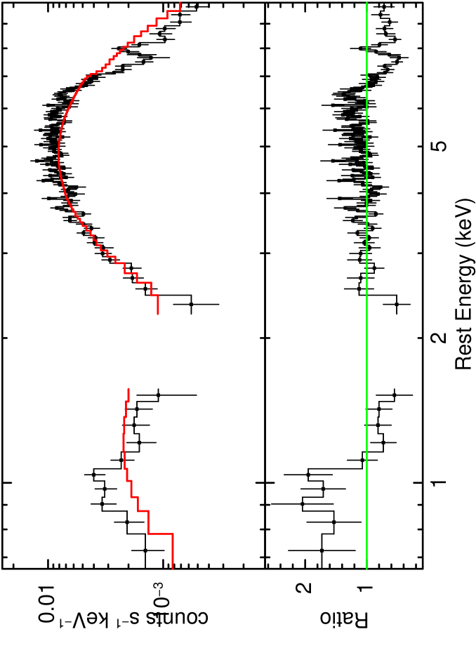
Figure 1: The upper panel shows the XIS-FI data (black data points) and a simple continuum model (shown in red), which is composed of an absorbed power-law component ($\Gamma=2$, $N_{\mbox{\scriptsize H}}\sim 2.5\times 10^{23}$ cm^-2) and a scattered soft power-law component. The lower panel shows the data/model ratio to this model. Clear residuals are visible in the soft X-ray band, due to possible thermal emission, and at the iron K-shell energy band. Besides a weak Fe K$\alpha$ emission line at $\sim 6.4$ keV, two strong absorption features are apparent at $\sim 7.4$ keV and at $\sim 8.5$ keV.

The addition of the Fe K$\alpha$ emission line improves the fit by $\Delta\chi^{2}/\rm{d.o.f.}=36.1/2$. The energy centroid is $E=6.40\pm 0.05$ keV and the equivalent width is $EW=150\pm 40$ eV, which is typical for mildly obscured Seyferts and suggests the presence of Compton-thick matter located out of the line of sight (Murphy & Yaqoob 2009). We therefore replaced the Gaussian emission line with a cold reflection component. For this component we adopted the pexmon model (Nandra et al. 2007), which includes the power law continuum reflected from neutral material as well as the Fe K$\alpha$, Fe K$\beta$, Ni K$\alpha$  emission lines and the Fe K$\alpha$ Compton shoulder. For the reflection component we assumed the same $\Gamma$ of the primary power-law component, an inclination angle of $60$ degrees, a high energy cutoff of 100 keV. We fixed the amount of reflection $R=\Omega/2\pi=1$ and allowed its normalisation to vary. However, even with this more complex model the true shape of the primary emission remains highly uncertain, because we lack any information on the emission above 10 keV and the X-ray spectrum is highly curved and dominated by the reprocessing features (see Fig. 1).

We thus decided to adopt the best fit photon index ($\Gamma=2.3$) that is obtained later with the simultaneous XMM-Newton & NuSTAR observation, where MCG-03-58-007 was detected with high signal to noise (S/N) up to 70 keV (see §3.2). The photon index was then allowed to vary to within $\pm 0.2$ of this value. From a statistical point of view this model provides an unacceptable fit ($\chi^{2}/\rm{d.o.f.}=329/206$) and the residuals still show a broad absorption feature at $E\sim 7.4$ keV and a second feature at $E\sim 8.5$ keV (see Fig. 2, upper panel). As expected $\Gamma$ hits the upper limit of the range ($\Gamma=2.5$), even allowing the slope of the soft scattered component to be independent from the shape of the hard component ($\chi^{2}=317.2/205$; $\Gamma_{\rm SOFT}>4$).

We then included in the model two Gaussian absorption lines, assuming a common line width. Since for the width we can only place a lower limit of $0.25$ keV, we subsequently fixed it to this value. The addition of the two Gaussian absorption lines improves the fit for a $\Delta\chi^{2}=63.5$ and $\Delta\chi^{2}=24.4$ for the 7.4 keV and the 8.5 keV feature, respectively. Thus, two absorption lines are both detected at a significance greater than 99.99%. The lower energy line ($E=7.42\pm 0.09$ keV) has an $EW=330\pm 70$ eV, while the higher energy one ($E=8.51\pm 0.15$ keV) has an $EW=320\pm 110$ eV. The most likely identifications of these features are blue-shifted $1s-2p$ transitions of Fe xxv or Fe xxvi (Tombesi et al. 2012; Gofford et al. 2013). If associated with Fe xxvi (which implies the smaller blue-shift) the two features can be explained with the presence of two highly ionised and high column density absorbers outflowing with $v_{1}\sim-0.07c$ and $v_{2}\sim-0.2c$.

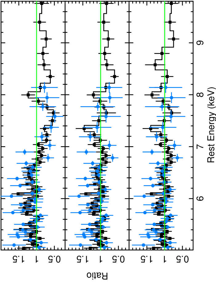
Figure 2: Zoom into the 5-10 keV residuals (XIS-FI data black data points, XIS1 light-blue) showing the improvement of the fit upon adding the ionised and outflowing absorbers. Upper panel: residuals to the continuum model after the inclusion of a cold reflection component ($\Gamma=2.5$). A strong (EW $\sim 330$ eV) absorption line is present at $E=7.4\pm 0.1$ keV, with a possible additional absorption feature at $E\sim 8.5\pm 0.1$ keV. Middle panel: residuals to the model, where we included one fast-outflowing ($v_{\rm out}/c=-0.076\pm 0.011$) ionised absorber; a second absorption feature is still present $E\sim 8.5$ keV. Lower panel: residuals to the best fit model, with two outflowing zones, where the photon index is now similar to the value obtained with the simultaneous XMM-Newton & NuSTAR observation ($\Gamma=2.2\pm 0.2$).

To self-consistently account for all these features we replaced the two Gaussian absorption lines with a multiplicative grid of photoionsed absorbers generated with the xstar photoionisation code (Kallman et al. 2004). Since the lines appear to be broad, we chose a grid that was generated assuming a high turbulence velocity ($v_{\rm turb}=10^{4}$ km s^-1) and optimised for high column density ($N_{\mbox{\scriptsize H}}=5\times 10^{22}$ - $2\times 10^{24}$cm^-2) and high ionisation (log$\,\xi=3-8$) absorbers. The grid was originally built for PDS 456 (N15, Matzeu et al. 2016) and assumes an intrinsically steep ionising continuum, where the intrinsic photon index is $\Gamma=2.4$ (N15). This choice is justified by the photon index measured for MCG-03-58-007 with NuSTAR, which is as steep ($\Gamma\sim 2.3$; see §3.2) as in PDS456. The inclusion of one fast-outflowing ionised absorber improves the fit by $\Delta\chi^{2}/\nu=68.9/3$. As expected from the parameters of the Gaussian absorption line model, we found that the absorber is outflowing with a velocity $v_{\rm out}/c=-0.075\pm 0.011$, is highly ionised log$\,\xi=5.5^{+0.5}_{-0.3}$ (e.g. consistent with the association of the $\sim 7.4$ keV feature with H-like iron) and has a high column density $N_{\mbox{\scriptsize H}}=6^{+6}_{-2}\times 10^{23}$ cm^-2.

Table 2: Summary of the two phase disk wind model for the Suzaku-2010 spectra. ^aThe ionisation of the second zone was tied to the ionisation of the lower velocity zone; if it is allowed to vary there is no improvement in the fit statistic. ^b The normalisation of the scattered power-law component is highly degenerate with the normalisation of the putative thermal emission component. The fluxes are corrected for the Galactic absorption, while the luminosities are intrinsic.

Model Component	Parameter	Value
Primary Power-law	$\Gamma$	$2.2_{-0.2}^{+0.2}$
	Norm. ($\times 10^{-3}$ ph keV-1 cm-2)	$3.5_{-1.2}^{+1.7}$
Scattered Component	Norm. ($\times 10^{-6}$ ph keV-1 cm-2) b	$8.9_{-5.8}^{+5.6}$
Thermal emission	kT (keV)	$0.64^{+0.07}_{-0.07}$
	Norm. ($\times 10^{-5}$ ph keV-1 cm-2)	$2.2_{-0.5}^{+0.5}$
Neutral absorber	$N_{\mathrm{H}}$ ($\times 10^{23}$ cm-2)	$2.7^{+0.3}_{-0.2}$
Zone 1	$N_{\mathrm{H1}}$ ($\times 10^{23}$ cm-2)	$7.8^{+3.9}_{-2.5}$
	log $\xi_{1}$	$5.54^{+0.29}_{-0.24}$
	$v_{\mathrm{out1}}/c$	$-0.075^{+0.010}_{-0.011}$
Zone 2a	$N_{\mathrm{H2}}$  ($\times 10^{23}$ cm-2)	$5.4^{+3.3}_{-3.0}$
	log $\xi_{2}$	$5.54^{t}$
	$v_{\mathrm{out2}}/c$	$-0.20^{+0.02}_{-0.02}$
Reflection	Norm. ($\times 10^{-4}$ ph keV-1 cm-2)	$7.8^{+9.1}_{-5.4}$
	$\chi^{2}/dof$	226.9/201
	$F_{(0.5-2)\mathrm{keV}}$(erg cm-2 s-1)	$5.4\times 10^{-14}$
	$F_{(2-10)\mathrm{keV}}$ (erg cm-2 s-1)	$2.0\times 10^{-12}$
	$L_{(0.5-2)\mathrm{keV}}$(erg s-1)	$1.7\times 10^{43}$
	$L_{(2-10)\mathrm{keV}}$ (erg s-1)	$1.4\times 10^{43}$

However, this ionised absorber is not able to account for the second absorption feature detected at $E\sim 8.5$ keV (see Fig. 2, middle panel), indeed the predicted blue-shifted Fe xxvi Ly$\beta$ ($E_{\rm Lab}=8.25$ keV), which is included in the model, would be too weak and centered at $\sim 8.8$ keV. We thus included a second ionised absorber (modelled with the same grid) and assumed that the two zones share the same ionisation, but allowed the $N_{\mbox{\scriptsize H}}$ and velocity to be different. Here, two absorbers are required to produce the final best-fit ($\chi^{2}=226.9/201$, $\Delta\chi^{2}=21.4$ for 2 d.o.f.) where no strong residuals are left (see Fig. 2, lower panel) and where $\Gamma$ is now reasonably constrained ($\Gamma=2.2\pm 0.2$). In Fig. 3 we show the resulting Suzaku spectrum with the best fit model overlaid, while the best fit parameters are reported in Table 2. Both zones of the ionised absorber are characterised by a high column density ($N_{\mathrm{H1}}=7.8^{+3.9}_{-2.5}\times 10^{23}$ cm^-2  and $N_{\mathrm{H2}}=5.4^{+3.3}_{-3.0}\times 10^{23}$ cm^-2), and are outflowing with $v_{\rm out1}=-0.075\pm 0.01c$ and $v_{\rm out2}=-0.20\pm 0.02c$. The high ionisation (log $\xi=5.5\pm 0.3$), outflow velocity and high velocity broadening are all indicative of a disk wind launched from within few tens to hundreds of $R_{\mathrm{s}}$ from the central SMBH (see §4.1).

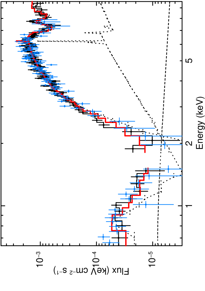
Figure 3: Suzaku data (XIS-FI data black data points, XIS1 light-blue) of MCG-03-58-007  when modelled with the two disk wind zones. The neutral absorber [$N_{\mbox{\scriptsize H}}=(2.7\pm 0.3)\times 10^{23}$cm^-2] is responsible for most of the curvature that is present below 6 keV. The imprints of the two phase disk wind are the two strong absorption features visible above 7 keV. A weak reflection component, which is most likely produced in the pc-scale putative torus, is present and mainly account for the Fe K$\alpha$ emission line. To generate the plot, we created fluxed spectra by unfolding the data against a $\Gamma=2$ power law model and then we overlaid the best-fit absorption model (red continuous line), which is reported in Table 2; i.e. the data were not unfolded against the absorption model.

3.2 Evidence for a variable absorber

3.2.1 The average XMM-Newton & NuSTAR spectra

We then considered the simultaneous XMM-Newton & NuSTAR observation of MCG-03-58-007 performed five years later and for simplicity we used only the EPIC-pn data for the XMM-Newton observation. The observations started almost at the same time (see Table 1), but the duration of the NuSTAR one extended beyond the XMM-Newton orbit. We binned both the NuSTAR FPMA/B spectra to a minimum of 100 counts per bin and the pn spectra to a minimum of 50 counts per bin. Although the NuSTAR observation has a longer duration ($\sim 300$ ksec) than the XMM-Newton one, we first jointly fitted the pn and the NuSTAR spectra extracted from the whole observation, allowing for a cross normalisation to account for variability and for instrumental calibration differences. As per the Suzaku spectra a model composed of an absorbed power-law component and a scattered soft power-law component (with the same $\Gamma$) provides a poor fit (with $\chi^{2}/{\rm d.o.f.}=1483.3/373$), leaving strong positive residuals above 10 keV and line-like residuals both in the soft X-ray as well as at the Fe K band. In Fig. 4 we show a comparison between the XMM-Newton & NuSTAR  and Suzaku data (the latter are included for comparison only). The overall spectral shape and fluxes are similar, with a pronounced curvature between 2 and 6 keV, which is due to the fully covering and neutral absorber.

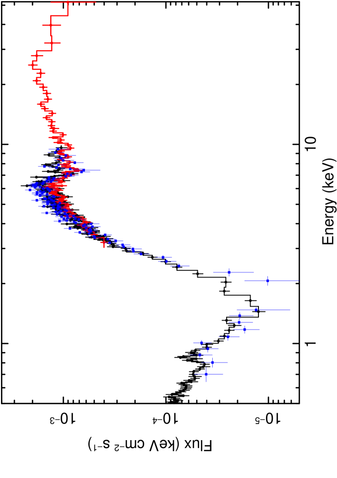
Figure 4: Comparison between the spectra of MCG-03-58-007 collected during the Suzaku (blue data points) and the simultaneous XMM-Newton (black circles points) & NuSTAR (red circles points) observations. The fluxed spectra have been created unfolding the data against a power law continuum with $\Gamma=2$. Note the similar level of the soft X-ray emission as well as the similar curvature in the 2-6 keV energy range, which is caused by the fully covering and neutral absorber ($N_{\mbox{\scriptsize H}}\sim 2\times 10^{23}$ cm^-2).

We thus added a neutral reflection component to the baseline continuum model. Since we are not interested here in the origin of the soft X-ray emission, which will be discussed in a forthcoming paper, we considered the EPIC-pn spectrum only above 2 keV and do not include in the model the scattered component. We note that the modelling of the soft X-ray emission does not impact the results obtained for the hard X-ray emission. Note that the soft X-ray spectrum is constant below 2 keV and it is dominated by emission lines, which likely originate in a photoionised emitter (e.g. the Narrow Line Region gas) with a small contribution from a collisionally ionised gas (Mazteu et al. in prep). For the reflection component, we adopted the pexmon model and we allowed only its normalisation to vary as we did for the Suzaku spectral analysis. Although the fit is still rather poor ($\chi^{2}/{\rm d.o.f.}=414.1/278$), several things can be already noted. First of all the X-ray photon index is no longer unusually steep ($\Gamma\sim 2.23\pm 0.06$). Secondly, the cross-normalisations between the XMM-Newton and NuSTAR spectra are $C_{\rm FPMA}=0.83\pm 0.03$ and $C_{\rm FPMB}=0.86\pm 0.03$, which are rather low for a simultaneous observation. Furthermore the NuSTAR data do not perfectly overlap with the XMM-Newton spectrum (see Fig. 4). Since the NuSTAR observation has a longer duration (see Table 1), we investigated whether during this observation the X-ray emission of MCG-03-58-007 varied and hence the averaged NuSTAR spectrum is fainter and harder than the pn spectrum.

3.2.2 The NuSTAR lightcurves: evidence for an eclipsing event

In Fig. 5 we show the combined FPMA & FPMB light curves extracted in the 3–6 keV (upper panel) and in the 20–40 keV band (middle panel) together with the hardness ratios (defined as $HR=\rm CR_{20-40\,keV}/CR_{3-6\,keV}$; lower panel) as a function of time. The light curves were extracted with a bin-size of 5814 sec corresponding to the NuSTAR orbital period. The two energy bands were chosen to track possible variations of the X-ray absorber (3–6 keV) and/or the primary continuum (20–40 keV). The inspection of the light curves shows that MCG-03-58-007  varied during the NuSTAR observation with a sharp drop in the 3–6 keV counts between 125-250 ksec, which is not accompanied by a similar drop in the hard X-ray counts. This is suggestive of an eclipsing event that strongly resembles the occultations seen in the light curves of NGC 1365 (Risaliti et al. 2009; Maiolino et al. 2010), which is often regarded as the prototype “changing-look" AGN. Similarly to what we witnessed for NGC 1365, the ingress of the absorber is rather sharp, while by the end of the observation the source begins to slowly uncover, as shown by the recovery in the 3–6 keV count rate after $\sim 250$ ksec. The hardness ratios light curve shows that MCG-03-58-007  becomes harder for almost half of the NuSTAR observation, with the HR increasing from $HR=CR_{\rm{20-40\,keV}}/CR_{\rm{3-6\,keV}}=0.17\pm 0.03$ to $HR=0.35\pm 0.06$.

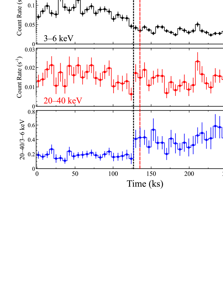
Figure 5: NuSTAR  light curves extracted (with a bin-size of 5814 sec) in the 3–6 keV (upper panel) and the 20-40 keV band (middle panel). The lower panel shows the HR light curve defined as $CR_{\rm{20-40\,keV}}/CR_{\rm{3-6\,keV}}$. While there are only small fluctuations in the 20–40 keV light curve, the 3–6 keV light curve presents a sharp drop at around 125 ksec (marked with the black dashed line) into the observation and a smooth increase at the end of the observation (at around 250 ksec, black dashed line). The HR light curve (lower panel) shows a sharp increase at 125 ksec, suggesting that we are witnessing an obscuration event. At 250 ksec the HR starts to decrease to almost the initial value. The red dashed line marks the end of the XMM-Newton observation at around 140 ksec.

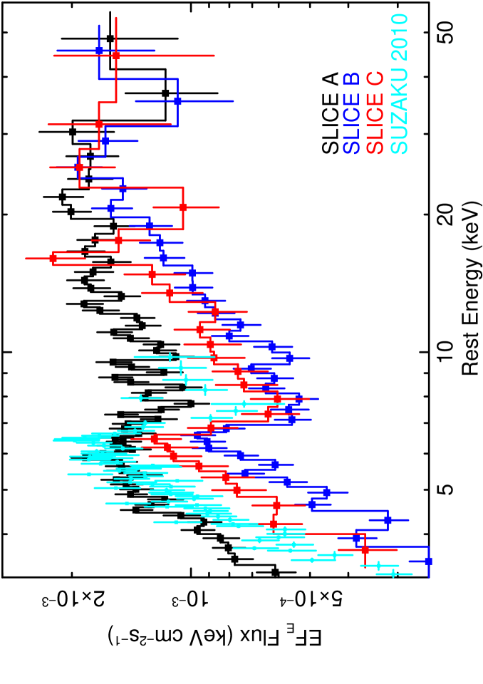
Figure 6: Comparison between the NuSTAR spectra of MCG-03-58-007, extracted following the HR light curve, and the Suzaku 2010 spectrum (shown in cyan). The NuSTAR spectra confirm that during the NuSTAR pointing we caught an occultation event. The first spectrum (sliceA, shown in black) is typical of a Compton thin state, while the X-ray spectrum of the second interval (sliceB from 125-250 ksec, blue data points) is similar to a Compton thick AGN. Although limited by the short net exposure time of the third (after 250 ksec) spectrum (shown in red), it is apparent that at the end of the observation MCG-03-58-007  begins to uncover. Note that the Suzaku spectrum is intermediate between the sliceA and sliceB spectra. To generate the fluxed spectra, we unfolded the data against a power-law continuum with $\Gamma=2$. FPMA and FPMB data are combined for plotting purposes.

We therefore extracted the XMM-Newton and NuSTAR spectra following the hardness ratio light curve shown in Fig. 5. Unfortunately when the variation occurred we are left with less than 10 ksec of the XMM-Newton observation. Since this latter EPIC-pn spectrum has a low S/N and since it covers only the beginning of the occultation, it was not considered for the time-resolved spectral analysis. All the spectra were binned to a minimum of 50 counts per bin. The resulting NuSTAR spectra are shown in Fig. 6 and confirm that during the observation we witnessed an occultation event. At the beginning of the observation MCG-03-58-007 shows a typical spectrum of a Compton thin AGN (black spectrum in Fig. 6). During the second half of the NuSTAR observation, the X-ray spectrum (blue spectrum in Fig. 6) is more curved and almost reminiscent of a highly obscured AGN. The spectra also confirm that we caught both the ingress of the obscuring cloud as well as the egress, as suggested by the hardness ratio light curve. Indeed, the third spectrum (shown in red in Fig. 6) is less obscured and MCG-03-58-007 starts to uncover in the 3–6 keV energy range. However, to investigate in detail the origin of the spectral variability, we considered only the first (0–125 ksec) and the second (125–250 ksec) intervals of the NuSTAR observation (hereafter sliceA and sliceB). The quality of the spectra of the third interval is too low for a detailed spectral analysis, because we have less than 15 ksec of net exposure time (per FPM detector).

3.2.3 Time-sliced spectra

In order to derive a baseline continuum model we first concentrated on sliceA. In Fig. 7 (upper panel) we show the data/model residuals for the pn spectrum, which offers the best spectral resolution, to a single absorbed power-law ($\Gamma=2.19\pm 0.06$) model over the 5–8 keV energy range ($\chi^{2}=400.8/276$). Both the Fe K$\alpha$ and Fe K$\beta$ emission lines are clearly visible as well as a weak absorption feature at the energy of one of the absorption lines detected in the Suzaku observation ($E\sim 7.4$ keV). Although the energy centroid of the absorption feature ($E=7.4\pm 0.1$ keV) is consistent with the lower energy absorption line detected in the Suzaku observation, the feature is now significantly weaker ($EW=64\pm 34$ eV), suggesting some variability of the disk wind. We then included in the model a Gaussian absorption line and a reflection component, for which we adopted the pexmon model and allowed only its normalisation to vary as we did for the Suzaku spectral analysis. This model already provides a reasonable description of the overall X-ray emission up to 65 keV ($\chi^{2}/{\rm d.o.f.}=335.2/272$, $\Gamma=2.35\pm 0.07$ and $N_{\mbox{\scriptsize H}}=(2.3\pm 0.1)\times 10^{23}$ cm^-2).

The residuals of sliceA and sliceB NuSTAR spectra against this continuum model (i.e. without any absorption feature) are shown in Fig. 8 (upper panel), where it emerges that the NuSTAR spectrum collected during sliceB is more absorbed, falling below the model up to 20 keV. Conversely, above 20 keV, where the spectra are dominated by the continuum emission, the sliceB spectrum is well predicted by this model. Thus, if present, variations of the primary emission cannot account for the sharp drop in the 3–6 keV light curve. The residuals of the more absorbed state are also far from featureless with two main absorbing structures between 7–12 keV. The lower energy structure is coincident with the $E\sim 7.4$ keV absorption feature detected in the Suzaku data, which appears to be much weaker in the sliceA spectrum. To further investigate these absorbing features, we then considered only sliceB and fitted a single absorbed power-law component. The ratio to this phenomenological model is shown in the lower panel of Fig. 8. A broad absorption trough is present blue-ward of the Fe K$\alpha$ emission line at around $\sim 7.4$ keV as well as at $\sim 10$ keV and above. We note that the overall profile is highly reminiscent of a P-Cygni profile from a wide angle outflow such as the one seen in the X-ray spectra of PDS456 (N15) and IRAS 11119+3257 (Tombesi et al. 2017), the prototype examples of a wide-angle fast disk-wind.

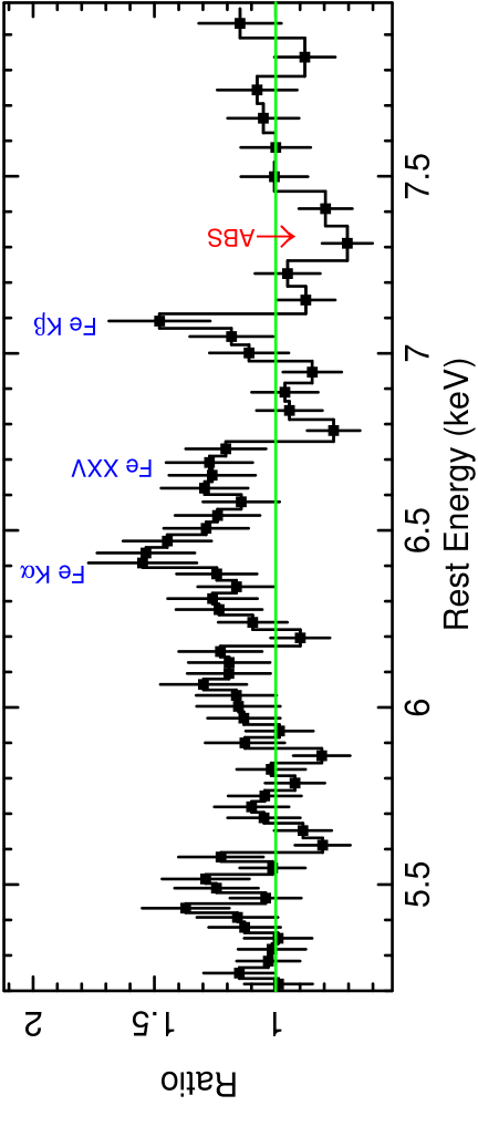
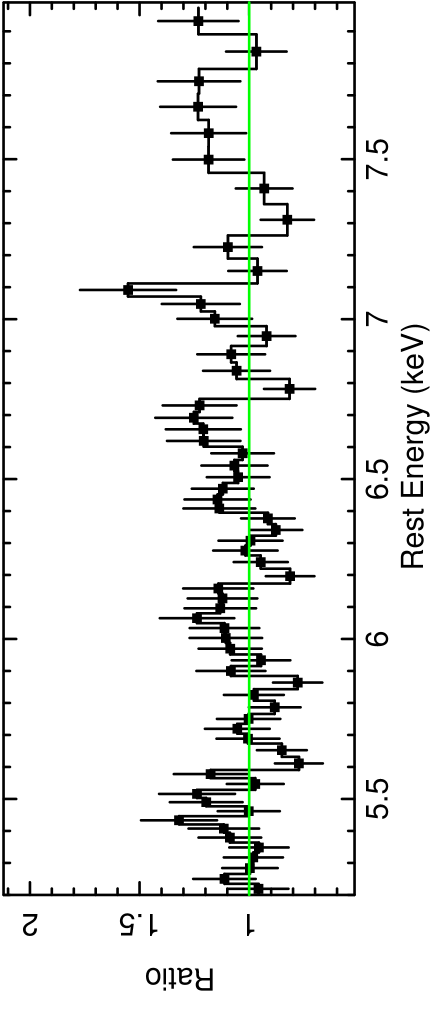
Figure 7: Zoom into the 5-8 keV EPIC-pn residuals of sliceA. Upper panel: residuals to the absorbed power-law model ($\Gamma=2.19\pm 0.06$). The residuals show the presence of the Fe K$\alpha$ and Fe K$\beta$ emission lines and a possible excess at the expected energy of the Fe xxv (labeled in blue). A weak absorption feature is present at the energy of one of the absorption lines detected in the Suzaku observation ($\Delta\chi^{2}/\mathrm{d.o.f.}=11.5/3$; $EW=64\pm 34$ eV; marked in red). Lower panel: EPIC-pn residuals for the two-zone disk wind model (see §3.2.4). Only a weak residual left is at the energy of the Fe K$\beta$ emission line, which is underestimated with the current pexmon model.

Although the high energies of these features suggest that they are most likely associated with blue-shifted Fe xxvi  resonance lines, and therefore with the presence of a highly ionised outflowing absorber, we tested alternative scenarios. We first investigated if variations of the primary continuum could explain the spectral changes assuming either a constant reflection component or a constant reflection fraction. The former case represents a scenario where the reflection is produced in distant material, such as the torus, which therefore does not respond to short time scale variations of the primary continuum. The latter case mimics a scenario where the reflecting material is much closer in and immediately reverberates the variations of the primary continuum. Neither of the two scenarios provide a satisfactory fit and both of them leaves strong residuals above 20 keV for sliceB. This is mainly caused by a factor of 2-3 decrease of the normalisation of the primary power-law component, which is required to account for the lower level of 2-10 keV emission seen during the second part of the observation. A strong decrease of the intensity of the primary power-law component is found even upon allowing for the neutral absorber to vary. The residuals of the NuSTAR spectra to the model of the first scenario including a variable neutral absorber ($\chi^{2}=470.1/345$ d.o.f.) are shown in Fig. 9 (upper panel). The model is unable to reproduce the curvature of the sliceB spectrum leaving positive residuals above 15 keV.

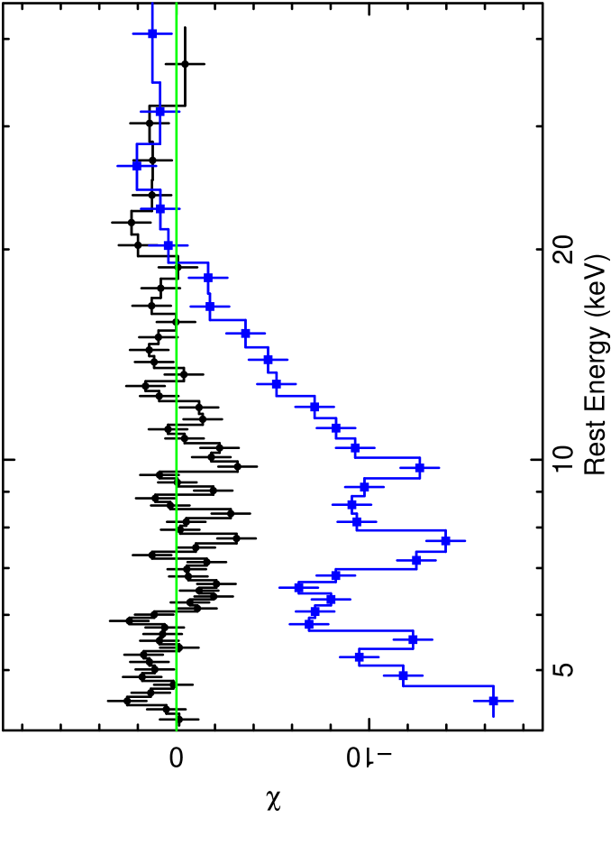
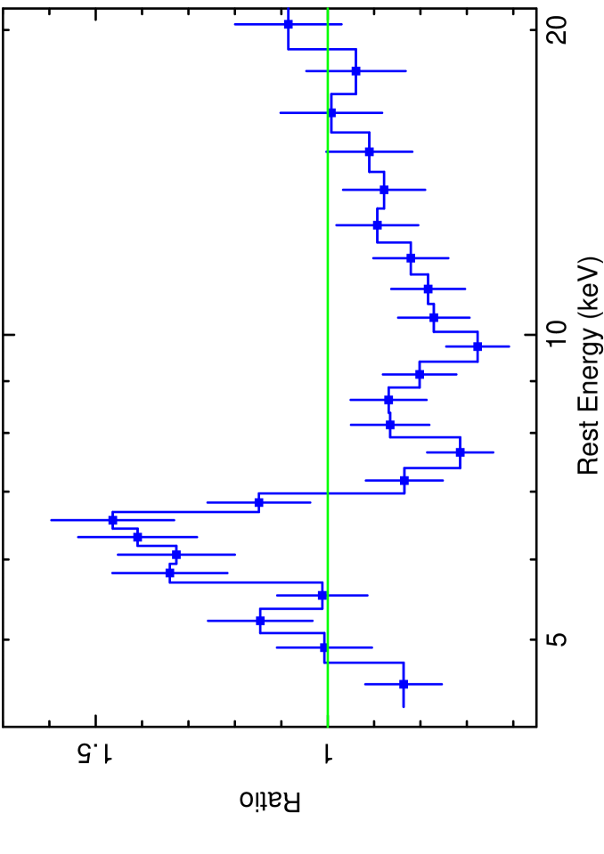
Figure 8: Upper panel: sliceA (black data points) and sliceB (blue data points) residuals to the best fit continuum model of sliceA. While only weak absorption structures are present in the residuals of the first part of the observation, two deep absorption troughs (at $E\sim 7.4$  keV and $E\sim 10$  keV) are evident in the residuals of the more absorbed state (blue data points). Lower panel: zoom into the 4–20 keV data/model ratio between the sliceB spectrum and an absorbed power-law continuum model. Two deep absorption features are evident in the data. The profile of the lower energy structure is highly reminiscent of a broad P-Cygni profile. FPMA and FPMB data are combined and rebinned to 120 counts per bin for plotting purposes.

We note that, since all these variable absorption models are neutral, none of them is able to account for the absorption features that are evident in the 7–12 keV residuals of sliceB. We then added to the baseline continuum model two Gaussian absorption lines, with variable depth between the two slices. As the width of both the Gaussian absorption lines is poorly constrained, they were fixed it to $0.1$ keV. The fit improves by $\Delta\chi^{2}=14.8$ and $\Delta\chi^{2}=27.1$ for the lower and higher energy features. The absorption lines are detected at $E=7.4\pm 0.1$ keV and $E=10.2\pm 0.1$ keV, respectively. Their equivalent widths, measured against the primary power-law component are $EW_{\rm 7.4\,keV}=70\pm 36$ eV and $EW_{\rm 10\,keV}=160\pm 100$  eV for slice A and moderately stronger in sliceB with $EW_{\rm 7.4\,keV}=170\pm 70$ eV and $EW_{\rm 10\,keV}=240\pm 130$ eV.

3.2.4 Modelling with a variable disk wind

A plausible scenario is that the variable absorber is the disk wind that was detected in the Suzaku observation. We thus included in the model the same multiplicative grid of photoionised absorbers adopted for the Suzaku spectra. We constrained the ionisation and outflow velocity of this ionised absorber to be the same between the slices and allowed only the column density to vary between the two slices. We did not allow the velocity to vary as the absorption features are seen at the same energy. We also allowed the neutral absorber and the normalisation of the primary power-law component to vary, while we assumed a constant reflection component. Upon adding this ionised absorber the fit improves by $\Delta\chi^{2}=60.9$ (for 4 d.o.f.). As expected the main driver of the spectral variability is an increase of the column density of this highly ionised (log $\xi=4.1\pm 0.1$) and outflowing ($v_{\rm out}=-0.12\pm 0.01c$) absorber from $N_{\rm HA}=1.5^{+0.8}_{-0.6}\times 10^{23}$cm^-2 to $N_{\rm HB}=(1.5\pm 0.2)\times 10^{24}$cm^-2. We note that a worse fit is obtained if we allow only the ionisation to vary instead of the $N_{\mbox{\scriptsize H}}$ ($\Delta\chi^{2}=18.4$). The neutral absorber is poorly constrained in sliceB, because with the NuSTAR data alone we can place only an upper limit of $N_{\rm HB}<1.1\times 10^{23}$cm^-2, while in sliceA we derive $N_{\rm HA}=(2.1\pm 0.2)\times 10^{23}$ cm^-2. However, if we assume a constant neutral absorber, a similar increase in $N_{\mbox{\scriptsize H}}$ is observed between sliceA and slice B ($\Delta N_{\mbox{\scriptsize H}}\sim 8\times 10^{23}$ cm^-2).This model can now better reproduce the different spectral curvature of sliceA and sliceB as well as the lower energy absorption structure at the Fe-K energy band. However, as expected from the energies of the two absorption features, this absorber cannot account for the structure at $\sim 10$ keV, because this feature is too deep to be explained with the corresponding higher order Fe xxv or Fe xxvi absorption lines. We thus included in the model a second ionised and outflowing absorber, allowing only its column density to vary between the slices. We also allowed this absorber to have a different ionisation of the first absorbing zone. The fit improves by $\Delta\chi^{2}=19.3$ for 4 d.o.f., which indicates that this additional zone is required at confidence level $>99.9$% according to the F-test. Since there is no evidence for variability of the column density of the faster zone ($N_{\rm H2A}=8.2^{+5.2}_{-3.2}\times 10^{23}$cm^-2 $N_{\rm H2B}>4\times 10^{23}$ cm^-2), we then tied its $N_{\mbox{\scriptsize H}}$ between the two slices ($N_{\rm H2}=8.1^{+4.8}_{-3.1}\times 10^{23}$cm^-2; $\chi^{2}/\nu=389.8/338$). This second and faster [$v_{\rm out2}=(-0.35\pm 0.02)\,c$] zone is characterised by a higher ionisation than the first zone log $\xi_{2}=6.2^{+0.2}_{-1.4}$.

We then tested if the observed variability could be instead explained with the presence of a variable and neutral partial covering absorber. We thus tied the column densities of the outflowing ionised absorbers and added a partial covering absorber, allowing the covering fraction to vary. From a statistical point of view this model returned an acceptable fit $\chi^{2}/\nu=379.4/337$. However, the $N_{\mbox{\scriptsize H}}$ of this absorber is found to be $>3.5\times 10^{24}$ cm^-2  and almost fully covering ($\sim 99$%) during sliceB. This implies a rather extreme and most likely unphysical scenario. Indeed, once the Compton scattering is taken into account for such a high $N_{\mbox{\scriptsize H}}$, the intrinsic 2–10 keV luminosity of MCG-03-58-007  would be of the order of $\sim 4\times 10^{44}$ erg s^-1  and thus too high when compared to our estimates of the bolometric luminosity ($L_{\rm{bol}}=1.6-3.4\times 10^{45}$ erg s^-1, see §4).

The relatively low ionisation of zone 1 (log$\xi=4.1\pm 0.1$) implies that the $\sim 7.4$  keV absorption line is associated with Fe xxv instead of Fe xxvi. This explains why we now derive a higher outflowing velocity ($v_{\rm out1}\sim-0.12\,c$) than with the Suzaku spectra ($v_{\rm out}\sim-0.075\,c$), which also displayed an absorption feature at $\sim 7.4$ keV. Note that if we assume for this zone the same ionisation derived with the Suzaku spectra the fit is worse by $\Delta\chi^{2}=20.2$. A possibility is that the cloud responsible for the occultation event is a denser clump with a lower ionisation. To test this scenario, we allowed also the ionisation of zone1 to vary between the slices. We also allowed the outflowing velocities to be different in order to adjust for the different ionisation. We found that, while in sliceA the ionisation could be similar to the Suzaku observation (log $\xi_{\rm A}=5.5_{-1.1}^{+1.2}$; $v_{\mathrm{out1}}=-0.07^{+0.03}_{-0.02}$), in the second part of the observation this zone has an ionisation of log $\xi=4.1_{-0.09}^{+0.09}$ and it is outflowing with $v_{\rm out}=-0.13\pm 0.02\,c$. This fit also confirms that the obscuring cloud has a column density of $N_{\rm H1B}=1.4_{-0.4}^{+0.2}\times 10^{24}$ cm^-2. The parameters for zone2 are almost identical to the previous model, because they do not depend on the lower velocity zone ($N_{\rm H2}=9.4^{+5.5}_{-3.4}\times 10^{23}$cm^-2, log $\xi=6.2_{-1.5}^{+0.2}$, $v_{\rm out2}=-0.35\pm 0.02c$).

Here, two highly ionised and variable absorbers are required to have an acceptable fit for the time-sliced spectra. The main contribution to zone 1 is the absorption structure at $\sim 7.4$ keV, as well as the spectral curvature below 10 keV, which becomes more pronounced during the second part of the observation and drives the increase in the column density. Conversely, zone 2, given its higher ionisation, does not imprint strong curvature to the observed spectra and mainly accounts for the higher energy absorption structure seen at $\sim 10$ keV (see Fig.  9, upper panel). The best fit parameters of this model are listed in Table 3, while the resulting residuals and spectra are shown in Fig.  9 (lower panel) and in Fig. 10, respectively. The final fit statistic ($\chi^{2}/\nu=382.7/336=1.14$) is now good and no strong residuals are present, with the exception of the weak absorption feature at $\sim 6.7-6.9$ keV, which is visible only in the pn data of sliceA. This feature could be a signature for a lower velocity and lower ionisation phase of the wind. We thus included in the model a third ionised absorber, which was also modeled with a multiplicative grid of photoionised absorbers generated with the xstar photoionisation code. We adopted a grid that has a lower turbulence velocity ($v_{\rm turb}=300$ km s^-1), because the absorption line seen in the pn appears to be narrow. The fit only marginally improves $\Delta\chi^{2}/\nu=10.7/3$, but confirms that an additional ionised absorber could be present; however, its parameters are poorly constrained ($N_{\mbox{\scriptsize H}}\sim 1\times 10^{23}$ cm^-2, log $\xi\sim 2.5$ and $v_{\rm out}=7000\pm 3500$  km s^-1). Note that the inclusion of this latter absorber does not affect the main parameters of the two fast zones of the disk wind. The Fe-K band residuals to this model are shown in the lower panel of Fig. 7.

Table 3: Summary of the two phase disk wind model applied to sliceA and sliceB (XMM-Newton & NuSTAR 2015 observation). ^a: The outflow velocity of this zone was allowed to vary to adjust for the different ionisation. ^b: the uncertainties on the column densities are determined for the best fit ionisation as they are highly degenerate with log$\xi$. ^c: the normalisation units are $10^{-3}$ ph keV^-1 cm^-2. ^t: denotes parameter was tied.

Model Component	Parameter	SliceA	SliceB
Primary Power-law	$\Gamma$	$2.28_{-0.07}^{+0.07}$	$2.28{{}^{t}}$
	Norm.c	$3.0_{-0.4}^{+0.4}$	$2.3_{-0.4}^{+0.5}$
Neutral absorber	$N_{\mathrm{H}}(\times 10^{23}$ cm-2)	$2.3^{+0.1}_{-0.1}$	$<1.1$
Zone 1a	$N_{\mathrm{H1}}$($\times 10^{23}$ cm-2)	$1.9^{+1.1}_{-0.7}$	$13.8^{+2.3}_{-3.5}$
	$log\xi_{1}$	$5.5^{+1.2}_{-1.1}$	$4.09^{+0.09}_{-0.09}$
	$v_{\mathrm{out1}}/c$	$-0.07^{+0.03}_{-0.02}$	$-0.13^{+0.02}_{-0.02}$
Zone 2b	$N_{\mathrm{H2}}$ ($\times 10^{23}$ cm-2)	$9.4^{+5.5}_{-3.4}$	$9.4^{t}$
	$log\xi_{2}$	$6.2^{+0.2}_{-1.5}$	$6.2^{t}$
	$v_{\mathrm{out2}}/c$	$-0.35^{+0.02}_{-0.02}$	$-0.35^{t}$
Reflection	Norm.c	$1.8^{+0.7}_{-0.6}$	$1.8^{t}$

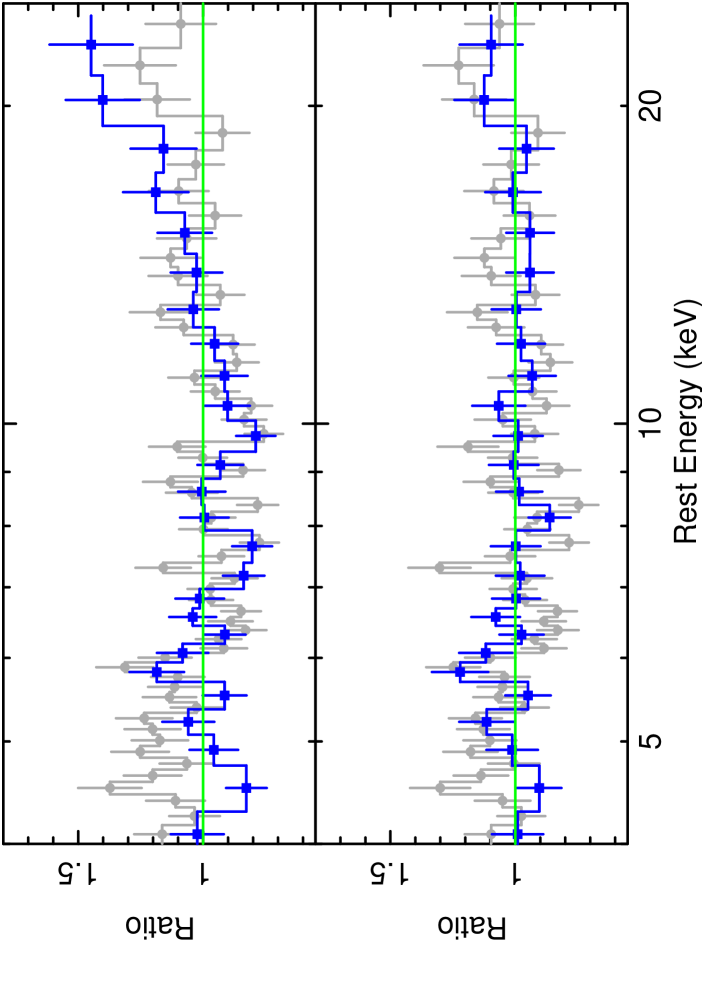
Figure 9: Zoom into the 4-25 keV range of the data/model residuals to the different variable absorber models fitted to the sliceA (grey data points) and sliceB (blue data points) spectra. The FPMA and FPMB spectra were co-added for plotting purposes. Upper panel: residuals to the model, where only the intensity of the primary power-law component and the amount of neutral absorption were allowed to vary. The model is unable to reproduce the curvature of the sliceB spectrum. Two main absorption structures are also visible at around $\sim 7.4$ keV (mainly in sliceB) and 10 keV. Lower panel: residuals to the two-zone disk wind model. After the inclusion of this ionised absorber, we can also reproduce the overall spectral curvature.

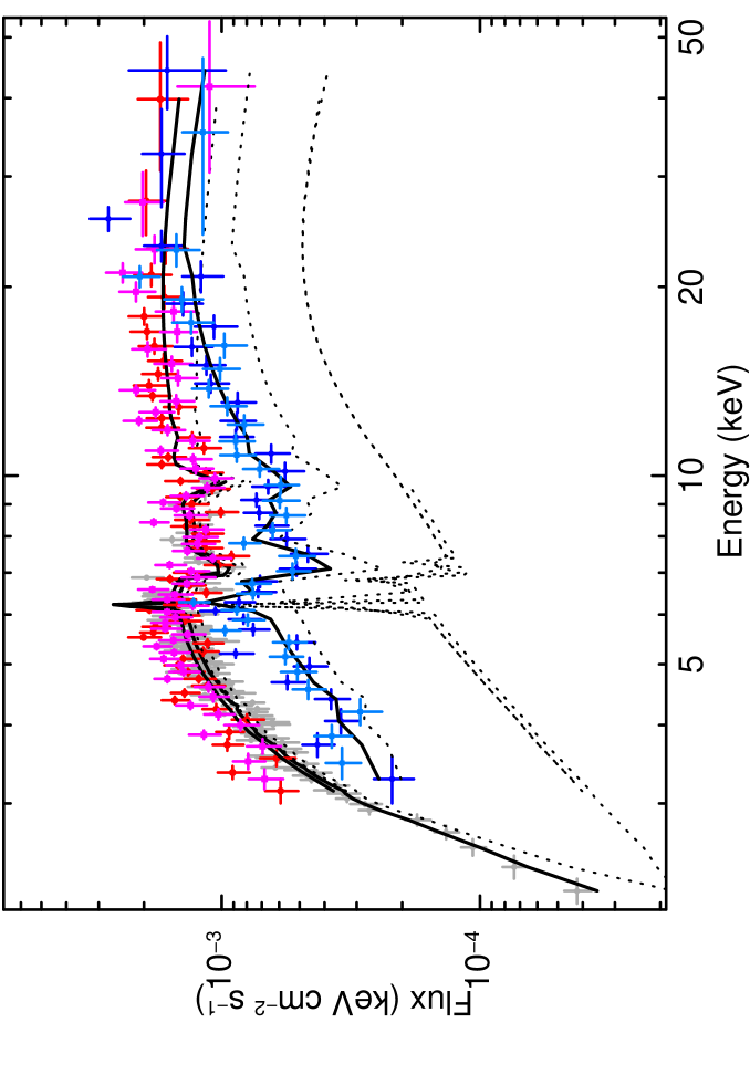
Figure 10: XMM & NuSTAR  sliceA and sliceB spectra. The spectra of the first part of the observations (pn grey, NuSTAR  FPMA red and FPMB magenta data points) and the second part of the observation (NuSTAR  FPMA blue and FPMB light blue data points) were fitted with a variable disk-wind model. The baseline continuum model is composed of an absorbed power-law component and reflected component. The $N_{\mbox{\scriptsize H}}$ of the neutral absorber and of the low-velocity ionised absorber (zone1) are allowed to vary. Zone1 is the main driver for the higher curvature observed below 20 keV during the second half of the observation, with a variation in the amount of absorption of $\Delta N_{\mbox{\scriptsize H}}\sim 1.4\times 10^{24}$ cm^-2. The fluxed spectra were generated as in Fig. 3.

4 Discussion and conclusion

We have presented the discovery of a new and highly variable disk wind. The disk wind has been discovered thanks to our long Suzaku observation, where two zones of a fast ($v_{\rm out1}=-0.075\pm 0.01\,c$ and $v_{\rm out2}=-0.2\pm 0.02\,c$) highly ionised absorber were revealed through the presence of two deep absorption features. This places MCG-03-58-007 among the fastest and potentially most powerful winds detected. Indeed, in only a handful of the disk winds discovered so far the velocity exceeds $0.2\,c$ (Gofford et al. 2015; Tombesi et al. 2012). In the follow up observation, performed simultaneously by XMM-Newton  & NuSTAR, we discovered a fast occultation event, which we ascribe to an increase of the $N_{\mbox{\scriptsize H}}$ of the slower zone of the disk wind from $N_{\mbox{\scriptsize H}}=1.9^{+1.1}_{-0.7}\times 10^{23}$ cm^-2 to $N_{\mbox{\scriptsize H}}=1.4^{+0.2}_{-0.4}\times 10^{24}$ cm^-2. The Suzaku observation has a duration of almost 200 ksec and shows strong variations, up to a factor of $\sim 2$, in the 2–10 keV X-ray band. However, without the bandpass above 10 keV, we cannot decouple whether the variations are due to continuum or column density changes. However, it is possible that during the Suzaku  observation our line of sight intercepted another clump of the wind with a $N_{\mbox{\scriptsize H}}$ that is intermediate between the $N_{\mbox{\scriptsize H}}$ measured in sliceA and sliceB. Indeed, as shown in Fig. 6, the Suzaku-spectrum falls between the NuSTAR spectra. To explore the properties of the disk wind detected in MCG-03-58-007, within the context of its possible impact on the host galaxy, we first need to derive a first order estimate of its mass outflow rate and kinetic output with respect to the bolometric and Eddington luminosity. To this end we need an estimate of the black hole mass and the possible launching radius of the disk wind.

An estimate of the black hole mass was derived using the relation between the SMBH mass and the stellar velocity dispersion ($\sigma$) of the host galaxy: log$M_{\mathrm{BH}}/M_{\odot}=8.12+4.24\times$log$(\sigma/200\,\rm{km\,s^{-1}})$ (Gültekin et al. 2009). An estimate of the stellar velocity dispersion can be obtained from the width of the narrow emission lines, like [OIII]$\lambda$5007Å, under the assumption that the Narrow Line Region gas is influenced by the potential of the host galaxy (Shields et al. 2003). The width of the narrow core only of the [OIII]$\lambda$5007Å  emission line was measured with the public spectrum of MCG-03-58-007 that is available in the final release of 6dF Galaxy Survey (DR3 6dFGS; Jones et al. 2009). Once corrected for the spectral resolution, we measured a width of $\sigma\sim 185$ km s^-1, which corresponds to an estimate of the SMBH mass of $\sim 1\times 10^{8}$ M_⊙.

The bolometric luminosity ($L_{\mathrm{bol}}$) can be derived from either the IR luminosity or from the luminosity of the [OIII]$\lambda$5007Å emission line, which are considered probes of the accretion disk luminosity. For the IR luminosity we used the Wide-field Infrared Survey Explorer (WISE) All-Sky catalogue (Wright et al., 2010). The W3 ($12\,\rm{\mu}$m) luminosity for MCG-03-58-007  is $L_{\rm WISE,3}=\nu_{\rm W3}\times L_{\rm W3}\sim 1.5\times 10^{44}$ erg s^-1, where $L_{\rm W3}$ and $\nu_{\rm W3}$ are the monochromatic luminosity and the central frequency correspondent to the W3 band. We then used the relation between $L_{\rm bol}$ and $L_{\rm WISE,3}$ derived by Ballo et al. (2014) for a sample of X-ray selected unabsorbed QSOs, which returned $L_{\rm bol}\sim 1.6\times 10^{45}$ erg s^-1. A similar value ($L_{\rm{bol}}\sim 3\times 10^{45}$ erg s^-1) is obtained from $\lambda L_{12\,\rm{\mu}\mathrm{m}}$, if we instead use the correlation derived for a sample of nearby Seyferts (see Fig.5 of Gandhi et al. 2009). Finally, from the observed L${}_{\rm{[OIII]}}=8.5\times 10^{41}$ erg s^-1reported by Wu et al. (2011) and assuming a bolometric correction of $L_{\rm bol}/L_{\rm{[OIII]}}=3500$ (Heckman et al. 2004 ), we derived $L_{\rm{bol}}\sim 3.4\times 10^{45}$ erg s^-1. Thus, while uncertain, the above estimates of $L_{\rm{bol}}=1.6-3.4\times 10^{45}$ erg s^-1  and the SMBH mass ($M_{\mathrm{BH}}\sim 10^{8}\,M_{\odot}$) suggest that MCG-03-58-007 has a moderate accretion rate ($\lambda_{\mathrm{Edd}}=L_{\mathrm{bol}}/L_{\mathrm{Edd}}=0.12-0.27$), which could be intermediate between a standard Seyfert and the high accretion rate objects like PDS 456.

4.1 Wind energetics, location and driving mechanisms

We now explore the main properties of the disk wind detected in MCG-03-58-007, focusing at first on the Suzaku observation. For simplicity we will assume a bolometric luminosity $\sim 3\times 10^{45}$ erg s^-1and $M_{\rm BH}\sim 10^{8}\,M_{\odot}$. During the 2010 observation two main absorbing zones were found, both characterised by a high ionisation (log$\xi=5.5\pm 0.3$) and a high column density ($N_{\mbox{\scriptsize H}}=5.4-7.8\times 10^{23}$ cm^-2). From the observed outflow velocity of the ionised gas we can infer a lower limit on the launching radius, by equating it to its escape radius $R_{\rm min}=c^{2}/v_{\rm out}^{2}R_{\rm s}$, where $R_{\rm s}\sim 3\times 10^{13}$ cm is the Schwarzschild radius for MCG-03-58-007. Thus, for the two components of the disk wind, we derive $R_{\rm min1}\sim 180\,R_{\mathrm{s}}$ ($\sim 5.4\times 10^{15}$ cm) and $R_{\rm min2}\sim 25\,R_{\mathrm{s}}$ ($7.5\times 10^{14}$ cm), for the slow ($v_{\rm{out1}}\sim 0.075\pm-0.01\,c$) and the fast ($v_{\rm{out2}}\sim-0.2\pm 0.02\,c$) component, respectively.

In order to infer the overall wind energetics and possible driving mechanism, the second main parameter that we need to quantify is the mass outflow rate ($\dot{M}_{\rm out}$). This can be derived with the equation $\dot{M}_{\rm{out}}=f\,\pi\,\mu\,m_{\mathrm{p}}\,M_{\rm BH}\,v_{\rm{out}}\,R\,N_{\rm{H}}$, which assumes a biconical geometry for the flow (Krongold et al. 2007), where $\mu=n_{\rm H}/n_{\rm e}=1.4$ for solar abundances and $R$ is the disk wind radius. The parameter $f$ is a function that accounts for the geometry of the system (i.e. inclination with respect to the disk and the line of sight). Since we do not know the exact geometry for MCG-03-58-007, we assumed $f\sim 1.5$, following the same arguments presented in Tombesi et al. (2013).

For the first zone (zone1), this yields a mass outflow rate of $\dot{M}_{\rm{out1}}\sim 1\times 10^{26}$ g s^-1 ($\sim 1.5M_{\odot}$ yr^-1) and a corresponding kinetic power of $\dot{E}_{\rm k1}\sim 2.4\times 10^{44}$ erg s^-1, which is approximately $\sim 8$% of the bolometric luminosity (or $\sim 2$% of $L_{\rm Edd}$). Thus, this zone is already energetically significant and can provide the feedback mechanisms between the central SMBH and the host galaxy, because it exceeds the theoretical thresholds for feedback ($\dot{E}_{\rm{kin1}}/L_{\rm{Bol}}\sim 0.5-5$ %, Hopkins & Elvis 2010; Di Matteo et al. 2005). It is interesting now to compare the outflow momentum rate, $\dot{p}_{\rm{out1}}=\dot{M}_{\rm{out1}}\,v_{\rm{out1}}$, with the radiation momentum rate $\dot{p}_{\rm{rad}}=L_{\rm{bol}}/c$. Although these estimates are rather uncertain, we found $\dot{p}_{\rm{out1}}\sim 2\times 10^{35}$ g cm s^-2 and thus of the same order of $\dot{p}_{\rm{rad}}$; this suggests that this zone could be radiation driven with a reasonable force multiplier. Although the fast component of the disk wind has a similar column density ($N_{\mbox{\scriptsize H}}=5.4^{+3.3}_{-3.0}\times 10^{23}$  cm^-2), the outflow rate is smaller ($\dot{M}_{\rm{out2}}\sim 2.6\times 10^{25}$ g s^-1), because the launching radius is smaller compared to zone1. However, the impact of this possible disk-wind component could be more important in terms of its feedback. Indeed, given its higher velocity ($v_{\rm{out2}}\sim-0.2\,c$), the kinetic power could be of the order of $5\times 10^{44}$ erg s^-1 that corresponds to $\sim 15$% of $L_{\rm bol}$.

Regarding the fastest zone (zone 2) detected during the XMM-Newton-NuSTAR observation, although the mass outflow rate could be of the same order of the one derived for the fast zone observed with Suzaku, as the launching radius is even smaller ($\sim 8\,R_{\mathrm{s}}$), the high velocity implies a high kinetic power ($\sim 40$% $L_{\rm Bol}$). However, all the parameters that we can derive for this zone are highly speculative, because its $N_{\mbox{\scriptsize H}}$ can be constrained only for a given ionisation (see Table 3; $N_{\rm H2}=8^{+5}_{-3}\times 10^{23}$cm^-2).

4.2 The occultation event: evidence for a clumpy disk wind

We will now discuss the properties of the slow component of the disk wind, which is found in both of the observations, within a clumpy disk wind scenario. First of all, following the same arguments discussed above, for the slow zone, detected in the first part of the XMM-Newton-NuSTAR observation, we derive: $R_{\rm min}\sim 200\,R_{\mathrm{s}}$ ($6\times 10^{15}$ cm), $\dot{E}_{\rm k}\sim 6\times 10^{43}$ erg s^-1 and $\dot{p}_{\rm{out}}\sim 5.5\times 10^{34}$  g cm s^-2. A possible scenario is that the disk wind detected at the beginning of the XMM-Newton-NuSTAR observation represents the most stable component of the wind. The absorption event that occurred during sliceB, can then be explained with an increase of its column density, when a denser region or clump of the wind moves across the line of sight. Assuming that its Keplerian (rotation) velocity is similar to the outflow velocity, we can derive the size scale of this denser clump. From the observed duration of the occultation $\Delta t\sim 120$ ksec and assuming $v_{\rm K}=v_{\rm out}=0.13\,c$, we derive a radial extent of the cloud of $\Delta R\sim 5\times 10^{14}$  cm ($\sim 16\,R_{\rm s}$). Then for the observed column density variation ($\Delta N_{\rm H}\sim 1.4\times 10^{24}$ cm^-2) and $\Delta R\sim 5\times 10^{14}$  cm, the density of the cloud is $n_{\rm e}=\Delta N_{\rm H}/\Delta R\sim 3\times 10^{9}$  cm^-3. From the definition of the ionisation parameter $\xi=L_{\rm{ion}}/n_{\rm e}R^{2}$ and assuming that the ionising luminosity is of the order of $10^{45}$ erg s^-1(i.e $\sim 1/3$ of the total bolometric luminosity), we derive a location for this eclipsing cloud of $R\sim 5\times 10^{15}$  cm ($\sim 170R_{\rm s}$) and thus consistent with the location of the bulk of the wind.

4.3 The Overall scenario of the Wind in MCG-03-58-007

MCG-03-58-007 is thus a new candidate for an extremely powerful and stratified disk wind. The two faster components of the disk wind, seen during the Suzaku and the XMM-Newton  & NuSTAR observations can be two different inner streamlines of the wind. One possibility is that during the 2015 observation the inner streamline of the wind is launched from closer in. The slow component of the wind (zone1) has been detected in both the deep observations, and it is outflowing with a velocity of the order of $\sim-0.1\,c$.

A possible scenario is that zone1 is the more long-lived component of the wind, which is likely launched from within a few hundreds of $R_{\rm s}$ from the central black hole. Nonetheless, this component is also highly inhomogeneous. Indeed, during the second part of the NuSTAR observation we witnessed an occultation, whereby our line of sight intercepted a clump or filament of the wind, leading to an increase in column density of $\Delta N_{\mbox{\scriptsize H}}\sim 1.4\times 10^{24}$ cm^-2. At face value the column density that is measured in sliceB would imply a large $\dot{M}_{\rm{out}}$ and a kinetic output $\dot{E}_{\rm k}\sim 8\times 10^{44}$ erg s^-1, and thus more difficult to be steadily driven. As observed this clump ($\Delta R=16R_{\rm s}$) corresponds to a short lived ($\Delta t\sim 120$ ksec) ejection event. This may suggests that additional accelerating mechanisms may be at work to produce such an ejection, like magnetic pressure (as in the MHD wind models; Fukumura et al. 2010), which then increase the momentum of the flow. We found no evidence that any of these variations could be a response to a different ionising luminosity; indeed, the 2–10 keV luminosities measured in 2010 and in 2015 are similar ($L_{2010}\sim 1.4\times 10^{43}$  erg s^-1  and $L_{2015}\sim 1.1\times 10^{43}$  erg s^-1).

5 acknowledgements

We thank the referee Anna Lia Longinotti for her useful comments that improved the paper. This research has made use of data obtained from Suzaku, a collaborative mission between the space agencies of Japan (JAXA) and the USA (NASA). Based on observations obtained with XMM-Newton, an ESA science mission with instruments and contributions directly funded by ESA Member States and the USA (NASA). This work made use of data from the NuSTAR mission, a project led by the California Institute of Technology, managed by the Jet Propulsion Laboratory, and funded by NASA. This research has made use of the NuSTAR Data Analysis Software (NuSTARDAS) jointly developed by the ASI Science Data Center and the California Institute of Technology. VB, GM, PS, AC and RD acknowledge support from the Italian Space Agency (contract ASI INAF NuSTAR I/037/12/0). VB also acknowledges financial support through grants NNX17AC40G and the Chandra grant GO7-18091X. GM is supported by a European Space Agency (ESA) Research Fellowship. JR acknowledges financial support through grants NNX17AC38G, NNX17AD56G and HST-GO-14477.001-A. C.C. acknowledges funding from the European Union’s Horizon 2020 research and innovation programme under the Marie Sklodowska-Curie grant agreement No. 664931

References

- Arnaud (1996) Arnaud, K. A. 1996, Astronomical Data Analysis Software and Systems V, 101, 17
- Ballo et al. (2014) Ballo, L., Severgnini, P., Della Ceca, R., et al. 2014, MNRAS, 444, 2580
- Blustin et al. (2005) Blustin, A. J., Page, M. J., Fuerst, S. V., Branduardi-Raymont, G., & Ashton, C. E. 2005, A&A, 431, 111
- Caccianiga et al. (2004) Caccianiga, A., Severgnini, P., Braito, V., et al. 2004, A&A, 416, 901
- Chartas et al. (2002) Chartas, G., Brandt, W. N., Gallagher, S. C., & Garmire, G. P. 2002, ApJ, 579, 169
- Crenshaw et al. (2003) Crenshaw, D. M., Kraemer, S. B., & George, I. M. 2003, ARA&A, 41, 117
- Dickey & Lockman (1990) Dickey, J. M., & Lockman, F. J. 1990, ARA&A, 28, 215
- Di Matteo et al. (2005) Di Matteo, T., Springel, V., & Hernquist, L. 2005, Nature, 433, 604
- Ferrarese & Merritt (2000) Ferrarese, L., & Merritt, D. 2000, ApJ, 539, L9
- Feruglio et al. (2015) Feruglio, C., Fiore, F., Carniani, S., et al. 2015, A&A, 583, A99
- Feruglio et al. (2017) Feruglio, C., Ferrara, A., Bischetti, M., et al. 2017, A&A, 608, A30
- Fukumura et al. (2010) Fukumura, K., Kazanas, D., Contopoulos, I., & Behar, E. 2010, ApJ, 715, 636
- Fukumura et al. (2017) Fukumura, K., Kazanas, D., Shrader, C., et al. 2017, Nature Astronomy, 1, 0062
- Gandhi et al. (2009) Gandhi, P., Horst, H., Smette, A., et al. 2009, A&A, 502, 457
- Gebhardt et al. (2000) Gebhardt, K., Bender, R., Bower, G., et al. 2000, ApJ, 539, L13
- George et al. (1998) George, I. M., Turner, T. J., Netzer, H., et al. 1998, ApJS, 114, 73
- Giustini & Proga (2012) Giustini, M., & Proga, D. 2012, ApJ, 758, 70
- Gofford et al. (2013) Gofford, J., Reeves, J. N., Tombesi, F., et al. 2013, MNRAS, 430, 60
- Gofford et al. (2014) Gofford, J., Reeves, J. N., Braito, V., et al. 2014, ApJ, 784, 77
- Gofford et al. (2015) Gofford, J., Reeves, J. N., McLaughlin, D. E., et al. 2015, MNRAS, 451, 4169
- Guainazzi & Bianchi (2007) Guainazzi, M., & Bianchi, S. 2007, MNRAS, 374, 1290
- Gültekin et al. (2009) Gültekin, K., Richstone, D. O., Gebhardt, K., et al. 2009, ApJ, 698, 198
- Harrison et al. (2013) Harrison, F. A., Craig, W. W., Christensen, F. E., et al. 2013, ApJ, 770, 103
- Heckman et al. (2004) Heckman, T. M., Kauffmann, G., Brinchmann, J., et al. 2004, ApJ, 613, 109
- Jones et al. (2009) Jones, D. H., Read, M. A., Saunders, W., et al. 2009, MNRAS, 399, 683
- Hopkins & Elvis (2010) Hopkins, P. F., & Elvis, M. 2010, MNRAS, 401, 7
- Kaastra et al. (2000) Kaastra, J. S., Mewe, R., Liedahl, D. A., Komossa, S., & Brinkman, A. C. 2000, A&A, 354, L83
- Kallman et al. (2004) Kallman, T. R., Palmeri, P., Bautista, M. A., Mendoza, C., & Krolik, J. H. 2004, ApJS, 155, 675
- Kaspi et al. (2002) Kaspi, S., Brandt, W. N., George, I. M., et al. 2002, ApJ, 574, 643
- Kato et al. (2004) Kato, Y., Mineshige, S., & Shibata, K. 2004, ApJ, 605, 307
- Kazanas et al. (2012) Kazanas, D., Fukumura, K., Behar, E., Contopoulos, I., & Shrader, C. 2012, The Astronomical Review, 7, 92
- King & Pounds (2003) King, A. R., & Pounds, K. A. 2003, MNRAS, 345, 657
- King (2010) King, A. R. 2010, MNRAS, 402, 1516
- King & Pounds (2015) King, A., & Pounds, K. 2015, ARA&A, 53, 115
- Krongold et al. (2007) Krongold, Y., Nicastro, F., Elvis, M., et al. 2007, ApJ, 659, 1022
- Laha et al. (2014) Laha, S., Guainazzi, M., Dewangan, G. C., Chakravorty, S., & Kembhavi, A. K. 2014, MNRAS, 441, 2613
- Magorrian et al. (1998) Magorrian, J., Tremaine, S., Richstone, D., et al. 1998, AJ, 115, 2285
- McKernan et al. (2007) McKernan, B., Yaqoob, T., & Reynolds, C. S. 2007, MNRAS, 379, 1359
- Mitsuda et al. (2007) Mitsuda, K., et al. 2007, PASJ, 59, 1
- Maiolino et al. (2010) Maiolino, R., Risaliti, G., Salvati, M., et al. 2010, A&A, 517, A47
- Matzeu et al. (2016) Matzeu, G. A., Reeves, J. N., Nardini, E., et al. 2016, MNRAS, 458, 1311
- Matzeu et al. (2017) Matzeu, G. A., Reeves, J. N., Braito, V., et al. 2017, MNRAS, 472, L15
- Mewe et al. (1985) Mewe, R., Gronenschild, E. H. B. M., & van den Oord, G. H. J. 1985, A&AS, 62, 197
- Murphy & Yaqoob (2009) Murphy, K. D., & Yaqoob, T. 2009, MNRAS, 397, 1549
- Nandra et al. (2007) Nandra, K., O’Neill, P. M., George, I. M., & Reeves, J. N. 2007, MNRAS, 382, 194
- Nardini et al. (2015) Nardini, E., Reeves, J. N., Gofford, J., et al. 2015, Science, 347, 860
- Piconcelli et al. (2005) Piconcelli, E., Jimenez-Bailón, E., Guainazzi, M., et al. 2005, A&A, 432, 15
- Pinto et al. (2017) Pinto, C., Alston, W., Parker, M. L., et al. 2017, arXiv:1708.09422
- Porquet et al. (2004) Porquet, D., Reeves, J. N., O’Brien, P., & Brinkmann, W. 2004, A&A, 422, 85
- Pounds et al. (2003) Pounds, K. A., Reeves, J. N., King, A. R., et al. 2003, MNRAS, 345, 705
- Proga et al. (2000) Proga, D., Stone, J. M., & Kallman, T. R. 2000, ApJ, 543, 686
- Proga & Kallman (2004) Proga, D., & Kallman, T. R. 2004, ApJ, 616, 688
- Reynolds (1997) Reynolds, C. S. 1997, MNRAS, 286, 513
- Reeves & Turner (2000) Reeves, J. N., & Turner, M. J. L. 2000, MNRAS, 316, 234
- Reeves et al. (2003) Reeves, J. N., O’Brien, P. T., & Ward, M. J. 2003, ApJ, 593, L65
- Reeves et al. (2009) Reeves, J. N., O’Brien, P. T., Braito, V., et al. 2009, ApJ, 701, 493
- Reeves et al. (2014) Reeves, J. N., Braito, V., Gofford, J., et al. 2014, ApJ, 780, 45
- Reeves et al. (2009) Reeves, J. N., O’Brien, P. T., Braito, V., et al. 2009, ApJ, 701, 493
- Reeves et al. (2014) Reeves, J. N., Braito, V., Gofford, J., et al. 2014, ApJ, 780, 45
- Reeves et al. (2018a) Reeves, J. N., Braito, V., Nardini, E., et al. 2018a, ApJ, 854, L8
- Reeves et al. (2018b) Reeves, J. N., Lobban, A., & Pounds, K. A. 2018b, ApJ, 854, 28
- Risaliti et al. (2009) Risaliti, G., et al. 2009, ApJ, 696, 160
- Rush et al. (1993) Rush, B., Malkan, M. A., & Spinoglio, L. 1993, ApJS, 89, 1
- Saez & Chartas (2011) Saez, C., & Chartas, G. 2011, ApJ, 737, 91
- Sim et al. (2008) Sim, S. A., Long, K. S., Miller, L., & Turner, T. J. 2008, MNRAS, 388, 611
- Shields et al. (2003) Shields, G. A., Gebhardt, K., Salviander, S., et al. 2003, ApJ, 583, 124
- Severgnini et al. (2012) Severgnini, P., Caccianiga, A., & Della Ceca, R. 2012, A&A, 542, A46
- Shu et al. (2008) Shu, X.-W., Wang, J.-X., & Jiang, P. 2008, Chinese J. Astron. Astrophys., 8, 204
- Sim et al. (2010) Sim, S. A., Proga, D., Miller, L., Long, K. S., & Turner, T. J. 2010, MNRAS, 408, 1396
- Spergel et al. (2003) Spergel, D. N., et al. 2003, ApJS, 148, 175
- Takahashi et al. (2007) Takahashi, T., et al. 2007, PASJ, 59, 35
- Tombesi et al. (2010) Tombesi, F., Cappi, M., Reeves, J. N., et al. 2010, A&A, 521, A57
- Tombesi et al. (2012) Tombesi, F., Cappi, M., Reeves, J. N., & Braito, V. 2012, MNRAS, 422, L1
- Tombesi et al. (2013) Tombesi, F., Cappi, M., Reeves, J. N., et al. 2013, MNRAS, 430, 1102
- Tombesi et al. (2015) Tombesi, F., Meléndez, M., Veilleux, S., et al. 2015, Nature, 519, 436
- Tombesi et al. (2017) Tombesi, F., Veilleux, S., Meléndez, M., et al. 2017, ApJ, 850, 151
- Turner et al. (1997) Turner, T. J., George, I. M., Nandra, K., & Mushotzky, R. F. 1997, ApJS, 113, 23
- Wilms et al. (2000) Wilms, J., Allen, A., & McCray, R. 2000, ApJ, 542, 914
- Wright et al. (2010) Wright, E. L., Eisenhardt, P. R. M., Mainzer, A. K., et al. 2010, AJ, 140, 1868-1881
- Wu et al. (2011) Wu, Y.-Z., Zhang, E.-P., Liang, Y.-C., Zhang, C.-M., & Zhao, Y.-H. 2011, ApJ, 730, 121