IFIC/18-20
Systematic classification of three-loop realizations of the Weinberg operator

Abstract

We study systematically the decomposition of the Weinberg operator at three-loop order. There are more than four thousand connected topologies. However, the vast majority of these are infinite corrections to lower order neutrino mass diagrams and only a very small percentage yields models for which the three-loop diagrams are the leading order contribution to the neutrino mass matrix. We identify 73 topologies that can lead to genuine three-loop models with fermions and scalars, i.e. models for which lower order diagrams are automatically absent without the need to invoke additional symmetries. The 73 genuine topologies can be divided into two sub-classes: Normal genuine ones (44 cases) and special genuine topologies (29 cases). The latter are a special class of topologies, which can lead to genuine diagrams only for very specific choices of fields. The genuine topologies generate 374 diagrams in the weak basis, which can be reduced to only 30 distinct diagrams in the mass eigenstate basis. We also discuss how all the mass eigenstate diagrams can be described in terms of only five master integrals. We present some concrete models and for two of them we give numerical estimates for the typical size of neutrino masses they generate. Our results can be readily applied to construct other $d=5$ neutrino mass models with three loops.

Keywords: Neutrino mass, radiative models, lepton number violation.

March 2, 2024

1 Introduction

The smallness of the observed neutrino masses has motivated many theoretical studies. For Majorana neutrinos, it can be understood from the Weinberg operator [1]:

$${\cal O}_{W}=\frac{c_{\alpha\beta}}{\Lambda}L_{\alpha}L_{\beta}HH$$ (1)

The classical seesaw picture of this operator [2, 3, 4, 5] corresponds to choosing for $\Lambda$ a very large scale, say $\Lambda\sim{\cal O}(10^{14})$ GeV, in which case neutrino masses are of the (sub-)eV order for $c_{\alpha\beta}\simeq{\cal O}(1)$. However, $c_{\alpha\beta}$ could be naturally much smaller than one, resulting in correspondingly lower values for the energy scale $\Lambda$ at which lepton number is violated. There are two simple ways of realizing such a suppression: (i) neutrino masses might be radiatively generated, in which case $c_{\alpha\beta}\propto 1/(16\pi^{2})^{n}$, where $n$ is the number of loops; (ii) higher d-dimensional operators might be responsible for neutrino mass generation. Note that such operators are always of the form ${\cal O}_{W}\times(H^{\dagger}H)^{\frac{d-5}{2}}$. In this paper we will follow the former idea and study systematically the decomposition of eq. (1) at three-loop order. For a recent systematic study of higher dimensional tree-level neutrino mass models see [6].

The idea that neutrino masses might be small due to their radiative origin is nearly as old as the seesaw mechanism itself, the Zee model being the classical example [7]. Many references can be found in the recent review [8]. See also [9] for general recipes on building loop neutrino mass models. For our work, the most relevant references in the literature are [10, 11, 12]: In [10] it was pointed out that there are just three variants of the seesaw at tree-level; references [11] and [12] gave a systematic decomposition of the Weinberg operator at 1-loop and 2-loop level, respectively. We make use of these results in the current work, which can be understood as a extension of [11, 12] to 3-loop diagrams. We also mention in passing that $d=7$ neutrino masses were studied systematically at tree-level in [13] and at the 1-loop level in [14]. The only genuine $d=7$ tree-level model was discussed in [15].

All the above papers follow a diagramatic approach to the classification of neutrino mass models. Alternatively, one can start from a list of non-renormalizable $\Delta L=2$ operators and find the ultra-violet completions (i.e. neutrino mass models) from a deconstruction of all operators. This approach has been used, for example, in [16, 17, 18], see also the discussion in [8].

Although understandably 3-loop neutrino mass models have received much less attention than lower order ones, still a number of papers on the subject can be found in the literature. An early example where the Weinberg operator is generated via a 3-loop diagram is the so-called KNT model [19]. In it, two charged scalar singlets plus a right-handed neutrino are added to the Standard Model (SM). Since the main motivation of this paper is to connect neutrino masses with dark matter, a $Z_{2}$ symmetry is added by hand under which one scalar and the right-handed neutrino are odd. The resulting 3-loop diagram is shown as model-2 in section 3 and we label its topology as $T_{5}$ in appendix A. The KNT model and a number of variants based on this original idea have been studied in several papers since then. For example, the authors of [20] added a second $N_{R}$ to explain the two distinct mass scales observed in neutrino oscillations. Other variants using $SU(2)$ triplets and quintuplets instead of singlets were discussed in [21] and in [22], respectively. Similar ideas revolving around the use of larger representations in the KNT model have been discussed in [23]. Also, the use of coloured particles in the KNT loop was studied in [24, 25, 26]. Yet another model variation with doubly charged singlets and doubly charged vector-like fermions was constructed in [27]. A scale-invariant version of the KNT model was presented in [28]. Finally, we mention that the phenomenology associated to the scalars in the KNT model and its triplet variant was discussed in [29]; for the collider phenomenology see [30, 31]. In all the above papers on the KNT model, the $Z_{2}$ symmetry was introduced by hand. In [32], however, $SU(2)_{L}$ septuplets are used (both scalar and fermionic), which lead to an accidental $Z_{2}$ symmetry and thus to automatically stable dark matter. There is also a very recent paper [33], based on the KNT topology, which uses (triplet) leptoquarks to explain also the anomalies observed in B-decays.

There are other 3-loop models based on topologies different from the one of the KNT model. The AKS model [34] requires two Higgs doublets, two $N_{R}$, a charged and a neutral scalar singlet. A $Z_{2}$, under which singlets are odd, eliminates the tree-level seesaw and stabilizes again the dark matter candidate. The AKS model generates two neutrino mass diagrams: They correspond to our diagrams $D_{6}^{M}$ and $D_{7}^{M}$ in figure 7, descending from topologies $T_{37}$ and $T_{22}$, respectively, shown in appendix A. The phenomenology and vacuum stability constraints for the AKS model have been studied in [35, 36, 37].

The same topologies and diagrams as in the AKS model appear also in [38]. However, the authors of [38] use doubly charged vector-like fermions and a scalar doublet with hypercharge $Y=3/2$ (plus the singlets of the AKS model). The diagrams $D_{6}^{M}$ and $D_{7}^{M}$ appear also in [39]. Here, however, these diagrams descend from our topologies $T_{40}$ and $T_{33}$. $D_{6}^{M}$ appears also in a model based on singlets [40], again descending from $T_{40}$. The last 3-loop model we mention is the one discussed in [41]. It contains a scalar septet and a fermionic quintuplet, generating the diagrams $D_{6}^{M}$ (from $T_{37}$) and $D_{7}^{M}$ (from $T_{32}$). The model contains an accidental $Z_{2}$, but still one needs to impose an additional $Z_{2}$ by hand.

Our classification scheme for the different topologies concentrates on identifying 3-loop genuine topologies, which are those associated with the dominant contributions to the neutrino mass matrix. We discuss thoroughly the concept of “genuineness” in section 2. There, we also define two classes of such topologies: Normal (or ordinary) genuine topologies (in total there are 44 of them) and special genuine topologies, which require very special fields (29 cases). The full list is given in appendix A.

As we will explain later, these special genuine topologies are associated to finite loop integrals, even though they generate some particular 3- or 4-point interaction at loop level. This happens because the corresponding tree-level renormalizable vertex vanishes due to the antisymmetric nature of some $SU(2)_{L}$ contractions. Our 29 special genuine topologies are of this type. However, there are some 3-loop models in the literature which also rely on such a loop-generated vertex, but do not (necessarily) fall into that list of 29 special topologies. Instead, those models use a symmetry to forbid the tree-level vertex, which is then generated at loop level, once the symmetry is (spontaneously) broken. The model presented in [42] falls into this class. (It generates diagram $D_{4}^{M}$, at the level of diagrams in the mass eigenstate basis.) Here, the tree-level vertex $e_{R}e_{R}k^{++}$ of the Babu-Zee 2-loop model [43, 44, 45] is forbidden by a global $U(1)$. Spontaneous breaking of this $U(1)$ to a $Z_{2}$ generates a Majorana mass for the $N_{R}$ (and produces a singlet Majoron) and generates this vertex at the 1-loop level. Similarly, a 3-loop diagram ($D_{5}^{M}$) appears in [46]. Note that, this type of models falls into the class called “fermionic cocktail” in [8]. We also mention [47], which studies a neutrino mass model based on an additional $SU(2)$ group, which leads to a 3-loop diagram with new vector bosons.

Then, there are also higher-dimensional 3-loop models. The authors of [48] presented a 3-loop model with neutrino masses at $d=7$. The so-called “cocktail model” [49] is actually a 3-loop model at $d=9$. (For a study of the phenomenology of the cocktail model see [50]). Note that we limit our deconstruction of 3-loop models to $d=5$ models. Thus, although the five master integrals defined in the appendix cover all possible 3-loop integrals, our topologies (and diagrams) are complete only for the $d=5$ case.

The rest of this paper is organized as follows. In section 2 we explain our classification scheme and how our results are obtained. All models which we classify as genuine have finite 3-loop integrals and thus do not need lower order counter terms for renormalization. We discuss that there is a further class of genuine topologies with finite 3-loop integrals, which correspond to loop generation of some 3- or 4-point vertices. We call these the special genuine topologies. We then show that the 73 genuine topologies (normal plus special ones) are associated to 374 diagrams in the weak basis, which get reduced to only 30 diagrams in the mass basis. We will discuss the dichotomy between normal and special topologies/diagrams in detail. We would like to point out that we are mostly interested in diagrams with new scalars (and/or new fermions). However, there could also be diagrams with vector particles, either the standard model W-boson or some exotic vector. While many of our results apply also to diagrams with vectors, we stress that due to a particular loophole in our procedure for finding genuine diagrams our list of genuine diagrams is incomplete for vectors. This is discussed in section 2 in more detail. In section 3 we show some example models, discussing them briefly. For two of them we perform also numerical calculations of the expected neutrino mass scale; they can easily reproduce the observed neutrino masses. We then close with a short discussion of our results. Several more technical aspects of our work are deferred to the appendix, where we show the genuine topologies and give the full definitions of the master integrals. A full list of the topologies and diagrams mentioned in our work can be found in [51].

2 Genuine topologies, diagrams and models

The following nomenclature will be used throughout the text. We shall call topologies to those Feynman diagrams where no property of the fields is considered (in graph theory, these are also known as undirected multigraphs). If scalars are differentiated from fermions, we will call them diagrams. If additionally the quantum numbers of the internal particles are specified, we will use the expression model-diagrams (or just model when it is clear from the context what we mean by this word).

Let us discuss now the concept of a genuine model-diagram, diagram and topology. Essentially, we want to identify this concept with those model-diagrams (plus their associated diagrams and topologies) for which the leading contribution to neutrino masses arises at 3-loops, without the need to introduce extra symmetries. Nevertheless, note that models with extra symmetries can be phenomenologically interesting; we provide one example of a 3-loop model-diagram with extra symmetries in section 3.

It is important to keep in mind that, in general, loop integrals have a finite and an infinite part. Infinite integrals require a lower order counter term in a consistent renormalization scheme. Thus, models with infinite $n$-loop amplitudes must necessarily also generate neutrino mass diagrams with less loops, and for that reason model-diagrams with an infinite amplitude are not genuine in our sense. However, certain diagrams lead automatically only to finite loop integrals, in which case it might be possible to build genuine model-diagrams from them.

Finiteness of the amplitude of a model-diagram is therefore a necessary condition for it to be genuine. However, it is not sufficient: it is also necessary to ensure that there are no other automatically generated model-diagrams with less loops. Consider neutrino masses generated via the dimension $d=5+2n$ operator

$$LLHH\left(H^{\dagger}H\right)^{n}$$ (2)

through a diagram with $\ell$ loops. It is expected that

$$M_{\nu}\sim\frac{1}{\left(4\pi\right)^{2\ell}}\left(\frac{\left\langle H\right\rangle}{\Lambda}\right)^{1+2n}\left\langle H\right\rangle\,.$$ (3)

As such, for diagrams with a characteristic scale $\Lambda\sim$ TeV, removing a loop ($\ell\to\ell-1$) and increasing the operator dimension by two units ($n\to n+1$) leaves $M_{\nu}$ with roughly the same value. So in order to have a dominant $\left(d,\ell\right)$ contribution to neutrinos masses, those with $\left(d^{\prime},\ell^{\prime}\right)=\left(d-2i,\ell-j\right)$ and $j>i$ should be absent. Genuine model-diagrams are those associated to these cases; in other words, the combination of fields participating in genuine model-diagrams must not be sufficient, by itself, to generate other more important neutrino mass contributions. For example, a model with a right-handed neutrino, $\nu_{R}$, will also give a $d=5$ tree-level contribution to the neutrino mass (unless an additional symmetry is used to eliminate some unwanted couplings), which will likely be the more important one. Stated in this way, genuineness is a concept which applies to model-diagrams. However, the list of such cases is infinite, in principle, as there are endless possibilities of assigning quantum numbers to the internal particles. We will therefore be interested in cataloguing those diagrams and topologies for which there exists at least one genuine model-diagram. These topologies and diagrams will be considered genuine themselves.

We found all such diagrams after a series of steps. First, using known algorithms (see for example [52]) we generate a list of all 3-loop connected topologies with 3- and 4-point vertices, and four external lines. This list contains a total of 4367 topologies. Only 3269 of them can accommodate 2 external fermion lines plus 2 external scalars using renormalizable interactions only.

Still at the level of topologies, we can already exclude a large number of these by applying the following straightforward criteria. We eliminate all cases with tadpoles (i.e., self-connecting vertices) and self-energies (i.e., 2-point subdiagrams with one or more loops), since these have always infinite parts in their loop integrals. This cut leaves us with 370 topologies.

We then eliminate the 1-particle reducible topologies, that is those topologies which become disconnected by cutting one of its lines. These cases can be discarded because the line which would disconnect the topology must have the quantum numbers to mediate type I, type II or type III seesaw (see fig. (1)).

Figure 1: A 1-particle reducible 3-loop topology. The line in the middle must correspond to one of the standard tree-level seesaw mediators, hence the topology is not genuine. The middle line is a fermion with the quantum numbers of $\nu_{R}\equiv(\boldsymbol{1},\boldsymbol{1},0)$ or $\Sigma\equiv(\boldsymbol{1},\boldsymbol{3},0)$ if it splits the external fields as $LH|LH$, or it is the scalar $\Delta=(\boldsymbol{1},\boldsymbol{3},-1)$ if the splitting is $LL|HH$.

This leaves us with 160 potentially genuine topologies, which can be divided in three classes: normal genuine topologies, special genuine topologies and non-genuine topologies. This division is done in steps.

There are those topologies for which an internal loop (or loops) can be compressed to a 3-point vertex (of the type fermion-fermion-scalar or scalar-scalar-scalar). For the remaining topologies, we find all valid diagrams, labelling internal lines as scalars or fermions in all possible ways, keeping externally exactly two scalars and two fermions. In this list we identify all diagrams with internal loops which can be compressed to a 4-scalar interaction. All diagrams without 3-point nor scalar 4-point loop subdiagrams fall into one of 44 topologies — see the counting on table 1. These we consider normal genuine diagrams and topologies. Their complete list is given in appendix A (the topologies) and in [51] (the topologies and the diagrams).

All topologies (connected, with 3 loops and 4 legs)	4367
Allow two external fermion lines	3269
No tadpoles	1056
No self-energies	370
1-particle irreducible	160
No 3-point loop subgraphs	70
No unavoidable 4-point scalar loop subgraphs	44

Table 1: Number of topologies, after the cumulative application of a series of cuts described in the text. Out of the initial 4367, only 44 have all the properties listed above: these are the normal genuine topologies. We would like to point out that dropping the requirement that a topology does no become disconnected by the cut of a single internal line (1-particle irreducibility), the final number of topologies would still be 44.

Consider first 3-point vertices. No matter what is the particle content of a model, if a loop with 3 external legs is allowed by symmetry, so is the trilinear vertex without the loop (see figure 2). Since this reasoning applies equally to fermion-fermion-scalar and to scalar-scalar-scalar vertices, this criterion can be defined at the level of topologies. For loops with 4 external legs, on the other hand, it is only possible to compress it to a renormalizable vertex if all external lines are scalars. Thus, this criterion needs to be used on diagrams, not topologies. The important point is that if a diagram has compressible subdiagrams (with 3 or 4 external legs), it cannot be genuine. We note that there is also the expectation of the converse: diagrams with incompressible loops are genuine, as there will be a choice of quantum numbers for the internal scalars and fermions such that there will be no other neutrino mass contribution with less loops (in appendix B we present an argument why we believe this is always true). That is why earlier we called them normal genuine diagrams.

Figure 2: Subparts of diagrams with loops and 3 external lines can be compressed into a 3-line vertex, reducing the number of loops of the diagram. For subparts with 4 external lines, this will only generate a renormalizable interaction if all external lines are scalars.

The usage of the word "normal" in this context is explained by the existence of exceptions to the above arguments. First of all, strictly speaking, this cut on 4-point vertices is only valid for diagrams without vector fields. Consider the diagram shown in figure 3: It has 3 external vector fields ($V$) and one scalar ($S$). Yet a term $VVVS$ is not Lorentz invariant, hence such a loop cannot be compressed into a renormalizable interaction (the effective interaction is $\partial VVVS$, of dimension 5). As a consequence of this, some otherwise non-genuine topologies might be classified as genuine if vector fields are used. We are mentioning this exception only for completeness, since we are interested in diagrams with fermions and scalars only.

Figure 3: Our procedure to obtain genuine 3-loop neutrino mass diagrams and topologies may not be valid in the presence of vector fields. In this example, a 1-loop fragment of a larger diagram cannot be contracted into a renormalizable point interaction, see text.

Figure 4: This 2-loop realization of the dimension five Weinberg operator illustrates a loophole in our automatized algorithm for finding genuine $n$-loops neutrino mass diagrams and topologies (we therefore track these special cases manually). In particular, if the scalar $S_{A}$ (or $S_{B}$) is the Higgs fields $H$, and $S_{B}$ (or $S_{A}$) is an $SU(2)$ singlet with the correct hypercharge, then there is no point interaction $HS_{A}S_{B}$. Hence, the existence of the left diagram does not imply that one can build the diagram on the right, with one loop less.

However, a second exception to the procedure used to obtain the previously mentioned 44 genuine diagrams is more subtle. To understand it, consider the 2-loop diagram in figure 4. The diagram appears to be non-genuine because it requires fields with quantum numbers such that they would have a renormalizable interaction $HS_{A}S_{B}$, which could be used to remove one loop from the diagram. In a sense, this is indeed always true: such trilinear combination of fields must be gauge invariant. Yet, $HS_{A}S_{B}$ might be identically zero for specific choices of $S_{A}$ and $S_{B}$. Take the case where $S_{A}$ is the Higgs field $H$, and $S_{B}$ is a scalar singlet with hypercharge -1. Then, $HHS_{B}\equiv 0$ because the $SU(2)$ singlet contraction of two doublets is antisymmetric. For particular choices of the quantum numbers of the remaining fields, one can in fact check that no $d=5$ 1-loop model is generated, hence the 2-loop diagram/topology in figure 4 is in fact genuine. This construction involving the use of repeated fields to forbid point-interactions (which otherwise would be allowed by their quantum numbers) can obviously be extended to 3-loop diagrams. These genuine 3-loop diagrams (topologies) which lead to non-genuine model-diagrams, unless very special choices of quantum numbers are made, we call the special genuine diagrams (topologies). Out of the 160 topologies mentioned above, 44 are normal genuine ones, and of the remaining 116 there are 29 which fall into this class. The complete list is shown in appendix A, where we also classify them according to which particular particle combination is needed to make the corresponding model genuine.

Note that, if we break down the fields into their components, the neutrino mass obtained from these special topologies arises from a difference of diagram amplitudes, with the negative sign(s) coming from the anti-symmetry of $SU(2)_{L}$ (and/or color) contractions. This is very clear, for example, in the 1-loop subdiagram in figure 4 (on the left), which must correspond to an $HHS_{B}$ interaction, as mentioned earlier. In the limit where the momenta flowing into these critical subdiagrams is small, the difference of amplitudes will approach zero. However, the momenta flowing into these subdiagrams is a loop momenta, hence the overall neutrino mass obtained from special genuine diagrams does not need to be small when compared to the mass obtained from normal genuine diagrams.

Figure 5: One example of a non-genuine but finite topology (to the left), generating the diagram on the right. See text.

The other 87 remaining topologies ($160=44+29+87$) generate non-genuine diagrams. Even so, it is important to note that some of these topologies (27 of them) may lead to non-genuine finite diagrams. These are diagrams for which an additional (broken) symmetry is always needed to forbid the otherwise allowed $\ell$-loop diagrams ($\ell<3$) that result from compressing one or more loops to a renormalizable vertex. We show an example of such a topology and corresponding non-genuine finite diagram in figure 5. In this diagram, the inner loop on the fermion line is an example of a compressible 3-point vertex. However, if this fermion is of Majorana type, one can add to the corresponding model an extra symmetry, for example a global $U(1)$ as in [42]. A SM singlet scalar can then be coupled to the Majorana fermion and assigned a charge under the $U(1)$. The tree-level coupling of the compressible inner loop could be forbidden in this way. Spontaneous breaking of this $U(1)\to Z_{2}$ by the vacuum expectation value (vev) of the singlet generates a Majorana mass term for the fermion and allows then this 3-loop diagram to exist.

We stress again that we do not consider this class to be genuine, as these models require extra symmetries (which need to be broken). Note that the symmetries can not be exact, otherwise the compressible loop is also forbidden by the symmetry. For the remaining 60 topologies in this non-genuine class all diagrams have infinite loop integrals. Due to the large number of topologies in this sub-class, we do not show them in this paper; they can be can found in [51].

We now return to the construction of the genuine diagrams. From the 44 normal genuine topologies, a total of 228 genuine diagrams can be built [51]. In figure 6 we show for one particular topology the possible diagrams, explaining graphically why several of them are not genuine. Diagrams with compressible loops are discarded in this set, as well as diagrams with non-renormalizable interactions. In this particular example, the topology has only two normal genuine diagrams. The remaining genuine diagrams, of the special kind, must be found carefully in a non-automated way (there are 146 of them, 66 of which have a special genuine topology, while the other 80 have a normal one).

Figure 6: There are two normal genuine diagrams associated to the topology shown in the top. There is also a total of 32 diagrams which can be drawn with a non-renormalizable fermion-fermion-scalar-scalar interaction. Finally, there are 4 diagrams which are also not normal genuine ones because it is possible to shrink a subpart of them into a renormalizable point interaction. (Note however that under some very specific circumstances, the third, the fifth and sixth diagrams in the top row can be genuine, hence they are considered special genuine diagrams.)

As a final step, the two external scalars standing for Higgs vev insertions are removed, and a list of 18 genuine (amputated) diagrams is obtained. These are shown in figure 7. In other words, the 228 diagrams in the electro-weak basis can be reduced to 18 diagrams in the mass eigenstate basis. To these one has to add the 12 diagrams in figure 8 which are obtained from special genuine diagrams. A visual summary of the steps described so far, as well as a counting of the genuine diagrams and topologies, can be found in figure 9. We state again, that while most of our results apply also to diagrams with vector bosons, our lists are not complete for vectors, due to the loophole discussed above in fig. 3.

We close this section by noting that the amplitudes of the 18+12 diagrams from figures 7 and 8 can be decomposed as linear combination of five master integrals [53]. Some of these master integrals admit an analytical solution, while others can only be solved numerically. A more detailed discussion about them is given in appendix C.

Figure 7: List of normal genuine diagrams in the mass basis. Note that the two external Higgs lines were removed: in general there is a many-to-one relation between the original diagrams and the amputated ones shown here. Diagrams in this list are referred to in the text as $D^{M}_{i}$, where $i$ is the number of the diagram shown here.

Figure 8: List of special genuine diagrams, with the external Higgs lines removed. Diagrams in this list are referred to in the text as $D^{M}_{i}$, where $i$ is the number of the diagram shown here.

Figure 9: Summary of the different types of diagrams and topologies. Out of thousands of topologies, only 160 are potentially interesting. They correspond to a total of 896 diagrams: 228 can provide dominant neutrino mass contributions without special considerations (normal genuine diagrams), and a further 146 can do so only with very special setups (special genuine diagrams). We call normal genuine topologies to those associated to at least one normal genuine diagram (there are 44); the special genuine topologies are the remaining cases which are associated to at least one special genuine diagram (there are 29). The remaining topologies are non-genuine but some of them (27) have at least one finite diagram. Once the external Higgs fields are removed, the 228 normal genuine diagrams become 18 amputated diagrams, while the remaining genuine diagrams in the weak basis yield 12 more amputated diagrams.

3 Examples

From the complete set of 228+146 genuine diagrams one can generate models by assigning quantum numbers to the internal fields following some basic rules. However, not all will lead to genuine 3-loop neutrino mass models. For that, one should guarantee the absence of fields that generate lower order contributions. For example $\nu_{R}$, $\Delta$ and $\Sigma$ of the basic three tree-level seesaws, or the scalar $S\equiv(\mathbf{1},\mathbf{4})_{3/2}$ together with the fermion $\Psi\equiv(\mathbf{1},\mathbf{3})_{1}$ from the $d=7$ tree-level BNT model [15]. Here, we introduced the notation $(\mathbf{SU(3)_{C}},\mathbf{SU(2)_{L}})_{Y}$ for the quantum numbers of internal particles. We will use this notation mostly in the figures. Note that we shortened this to $\mathbf{SU(2)_{L}}_{Y}$ for colourless particles. Thus, for example, a fermionic $\mathbf{1}_{0}$ corresponds to a right-handed neutrino $\nu_{R}$. As discussed above, it is however possible in many cases to construct models that avoid lower order diagrams, despite the use of particles such as $\nu_{R}$, by adding additional symmetries by hand to the model. We will show one example of such a model below. In that case we add a superscript $\omega$ to the particle quantum numbers to indicate which particles are charged under the new symmetry. The simplest possibility is usually a $Z_{2}$.

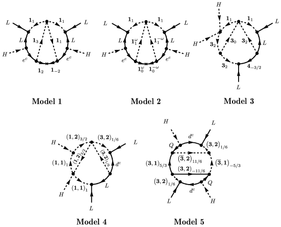
Figure 10: Five examples of three-loop $d=5$ genuine neutrino mass models.

Since there are endless possibilities for the quantum numbers of the internal fermions and scalars, the number of genuine models is infinite. Here we will just show a few basic examples: Five comparatively simple models are shown in fig. 10. Let us discuss them briefly.

Model 1, based on the same diagram as the KNT model, can be considered as one of the simplest genuine 3-loop models possible. The diagram needs only three singlets (two different scalars and one vector-like fermion) and no additional symmetry to produce a non-zero neutrino mass. All other models that we found need either (i) larger $SU(2)_{L}$ representations and/or (ii) a larger number of beyond SM fields and/or (iii) an additional symmetry to avoid lower order diagrams.

Model 2 is the simplest realization of the KNT model. It also contains only three different singlets, as is the case for model 1. However, the KNT model needs an extra symmetry to avoid a tree-level seesaw contribution from the fermionic singlet (recall that $\mathbf{1}_{0}\equiv\nu_{R}$). We indicate the particles transforming non-trivially under the new symmetry, by writing their charge $\omega$ as a superscript. Note that for the simplest case of a $Z_{2}$ this simply reduces to the particles in the innermost loop to being odd, while the rest of the diagram contains only particles transforming even. As we mentioned earlier in the introduction of the paper, there is a number of variations of this diagram in the literature containing larger $SU(2)_{L}$ representations in the loops and colored particles as well.

We have chosen model 3 to show how larger $SU(2)_{L}$ representations can also play a natural role in 3-loop neutrino mass models. This model is associated to topology $T_{3}$, being the first 3-loop model to do so in the literature, as far as we know. There are three new scalars, ${\bf 3}_{0}$, ${\bf 3}_{2}$, ${\bf 1}_{1}$ and one new fermion ${\bf 4}_{-3/2}$ (plus its vector partner). The model contains a triply-charged “leptonic” fermion as well as a triply charged scalar, and thus it should lead to a very rich accelerator phenomenology.

The second row in figure 10 shows two models with coloured fields. Here, we have chosen the simplest possibilities for colour, i.e. we use only triplets. Variants with larger colour representations could be created in a straightforward manner. In the diagram of model 4, colour runs only in one of the loops. This model has again only three new fields. However, in contrast to models 1–3, here all new fields are scalars. The scalar $(\mathbf{3,2})_{1/6}$ is a lepto-quark, thus standard LHC searches for these particles should put bounds on this model. Note that model 4 descends from our topology $T_{1}$ (we have not found any model with this topology in the literature). Model 5 is a second example with coloured particles: it needs 5 exotic fields, but no additional symmetry. Note again that the exotic fermions in this model, $({\bf 3},{\bf 2})_{-11/6}$ and $({\bf 3},{\bf 1})_{5/3}$, both must be vector-like.

In the following we will discuss models 1 and 5 in more detail, including a numerical calculation of the relevant 3-loop integrals. We will only consider the unrealistic case where one neutrino is massive, adding just one generation of every new field for simplicity. Therefore, our results should be understood as estimates of the typical scale of the neutrino masses and not as a prediction for their exact values. Note, however, that it is possible to fit all neutrino oscillation data, including the mixing angles, in radiative models. Usually, adding more copies of the exotic fermions is enough (we discuss this briefly at the end of this section).

Also, unless we say otherwise, in the following all dimensionless couplings are set to one and, in this simplified setup, we will not put a hierarchy nor flavour structure in the indices of the Yukawa couplings. (This is done for simplicity; it is not a requirement/constraint on the models.) When there are no analytical solutions, the calculations for the three-loop integrals have been done numerically with the code pySecDec [54]. For detailed definitions of the loop integrals see the appendix C.

3.1 Model 1

Fields	$SU(3)_{C}$	$SU(2)_{L}$	$U(1)_{Y}$
$S_{1}$	1	1	1
$S_{2}$	1	1	3
$F$	1	1	2

Table 2: Quantum number assignments for the beyond-the-SM fields of model 1 (compare to figure 10).

Model 1 contains the SM fields plus the ones given in table 2. The fermion $F$ has a vector partner $\overline{F}$, which is not explicitly shown in the table. The neutrino mass in model 1 is generated from the following terms in the Lagrangian:

$$\mathscr{L} =\mathscr{L}_{SM}+Y_{1}\overline{L^{c}}LS_{1}+Y_{2}\overline{F}e^{c}S_{1}+Y_{3}Fe^{c}S_{2}^{\dagger}+\lambda_{S}S_{2}(S_{1}^{\dagger})^{3}+\textrm{h.c.}$$

$$+m_{1}^{2}S_{1}^{\dagger}S_{1}+m_{2}^{2}S_{2}^{\dagger}S_{2}+M\overline{F}F+\cdots.$$ (4)

Other quartic terms in the scalar potential (such as $H^{\dagger}HS^{\dagger}S$) are not explicitly given here, as they will only result in uninteresting corrections to the scalar masses. It is worth mentioning that $Y_{1}$ in eq. (3.1), in principle, is a $3\times 3$ antisymmetric matrix. This fact is important if one wants to fit the complete neutrino oscillation data (see the discussion at the end of this section).

The mass diagram of model 1 in figure 10 shows that the neutrino mass is proportional to the product of two masses of SM charged leptons. Considering the dominant contribution with two $\tau$ leptons running in the loop, the neutrino mass matrix is then calculated straightforwardly as:

$$(M_{\nu})_{\alpha\beta}=-\frac{3!}{(16\pi^{2})^{3}}\lambda_{S}\frac{m_{\tau}^{2}}{M}\left[(Y_{1})_{\alpha\tau}(Y_{2})_{\tau}(Y_{3})_{\tau}(Y_{1})_{\tau\beta}\;+\;(\alpha\leftrightarrow\beta)\right]\;F_{loop}\!\left(x_{1},x_{2}\right).$$ (5)

After EWSB, in the mass eigenbasis, model 1 generates the diagram $D_{3}^{M}$ in figure 7 with a mass insertion in each of the three internal fermions. From the diagram, and assigning momenta to the internal fields, we get the following expression for the loop function $F_{loop}$, which is given by a dimensionless integral:

$$F_{loop}\!\left(x_{1},x_{2}\right)=\!\!\!\!\!\!\iiint\limits_{(k_{1},k_{2},k_{3})}\!\!\!\frac{1}{[k_{1}^{2}][k_{1}^{2}-x_{1}][k_{2}^{2}][k_{2}^{2}-x_{1}][k_{3}^{2}-1][(k_{2}-k_{3})^{2}-x_{1}][(k_{3}-k_{1})^{2}-x_{2}]}.$$ (6)

Here $m_{\tau}$ was neglected, while the other masses were normalized to the vector-like mass $M$ of the field $F$:

$$x_{1}=\frac{m_{1}^{2}}{M^{2}},\;x_{2}=\frac{m_{2}^{2}}{M^{2}}.$$ (7)

We also used the short-hand notation

$$\int\limits_{k}\equiv(16\pi^{2})\int\frac{d^{4}k}{(2\pi)^{4}}.$$ (8)

For the full decomposition of $F_{loop}\!\left(x_{1},x_{2}\right)$, in terms of master integrals, suitable for numerical evaluation, see appendix C.

Figure 11: The neutrino mass scale in model 1 for a few sample choices of parameters, see text for details.

In figure 11 we show the neutrino mass scale for different choices of parameters. For the calculation we have taken all masses of the new scalar singlets equal, i.e. $m_{1}=m_{2}=m_{S}$. As can be seen from eq. (5), $M_{\nu}$ is proportional to the fourth power of the Yukawas. For masses of order $\mathcal{O}(1)$ TeV one can reproduce the neutrino atmospheric scale ($\sim 0.05$ eV) with Yukawas $\mathcal{O}(10^{-2}-10^{-1})$.

The dependence of the neutrino mass on the masses of the fields in the loop is also understood straightforwardly. From the diagram of model 1 in the mass eigenbasis, it is straightforward to see that the neutrino mass should scale as:

$$M_{\nu}\sim m_{\tau}^{2}\frac{M}{\Lambda^{2}},$$ (9)

where $\Lambda$ is some characteristic energy scale. As the loop function contains only two mass scales, i.e. $m_{S}$ and $M$ (neglecting $m_{\tau}$), for $m_{S}\gg M$ the neutrino mass decreases with $1/m_{S}^{2}$, while for small scalar masses one obtains a constant value (for a fixed $M$).

In summary, as figure 11 shows, the correct neutrino mass scale is obtained in this model for a wide range of masses. In one extreme case, the new physics scale can be as high as $10^{3}$ TeV if all Yukawas are order one. On the other hand, even for masses $M$ and $m_{S}$ of the order of $1$ TeV, Yukawa couplings can be as large as ${\cal O}(0.1)$.

3.2 Model 5

We have performed an analogous study for model 5 of figure 10. In the mass eigenbasis, the neutrino diagram corresponds to diagram 10 in figure 7 with a mass insertion on both d-quark internal lines.

Fields	$SU(3)_{C}$	$SU(2)_{L}$	$U(1)_{Y}$
$S_{Q}$	3	2	1/6
$S_{1}$	3	1	5/3
$S_{2}$	3	2	-11/6
$F_{1}$	3	1	5/3
$F_{2}$	3	2	-11/6

Table 3: Quantum numbers of the new fields given in model 5 (see figure 10).

The new fields present in the model are listed in table 3. Among others, the Lagrangian contains the following interactions:

$$\mathscr{L} =\mathscr{L}_{SM}+Y_{1}Ld^{c}S_{Q}+Y_{2}QF_{1}S_{2}+Y_{3}QF_{2}S_{1}+Y^{L}_{4}\overline{F_{1}}\,\overline{F_{2}}S_{Q}^{\dagger}+Y^{R}_{4}F_{1}F_{2}S_{Q}+\mu_{S}S_{Q}^{\dagger}S_{1}^{\dagger}S_{2}^{\dagger}+\textrm{h.c.}$$

$$+M_{F_{1}}\overline{F_{1}}F_{1}+M_{F_{2}}\overline{F_{2}}F_{2}+m_{S_{Q}}^{2}S_{Q}^{\dagger}S_{Q}+m_{S_{1}}^{2}S_{1}^{\dagger}S_{1}+m_{S_{2}}^{2}S_{2}^{\dagger}S_{2}+\cdots.$$ (10)

Additional quartic terms in the scalar potential coupling the new scalars and the higgs field are not written down explicitly.

Similarly to model 1, the neutrino mass in model 5 is proportional to the product of two d-quark masses. Thus, one expects the dominant contribution will be proportional to the mass of the bottom quark squared:

$$(M_{\nu})_{\alpha\beta} =-\frac{12\mu_{S}}{(16\pi^{2})^{3}}\frac{m_{b}^{2}}{m_{S_{Q}}^{2}}\left[(Y_{1})_{\alpha b}(Y_{2})_{b}(Y_{3})_{b}(Y_{1})_{b\beta}\;+\;(\alpha\leftrightarrow\beta)\right]$$ (11)

$$\times\left[Y^{L}_{4}F_{L}(x_{1},x_{2},x_{3},x_{4})+Y^{R*}_{4}F_{R}(x_{1},x_{2},x_{3},x_{4})\right]$$

where

$$F_{L}(x_{1},x_{2},x_{3},x_{4})= \;\;\;\!\!\!\!\!\!\iiint\limits_{(k_{1},k_{2},k_{3})}\!\!\!\frac{\sqrt{x_{1}x_{3}}}{[k_{1}^{2}][k_{1}^{2}-1][k_{2}^{2}][k_{2}^{2}-1][k_{3}^{2}-x_{1}][k_{3}^{2}-x_{2}][(k_{2}-k_{3})^{2}-x_{3}][(k_{3}-k_{1})^{2}-x_{4}]},$$ (12)

$$F_{R}(x_{1},x_{2},x_{3},x_{4})= \;\;\;\!\!\!\!\!\!\iiint\limits_{(k_{1},k_{2},k_{3})}\!\!\!\frac{\not{k_{3}}(\not{k_{2}}-\not{k_{3}})}{[k_{1}^{2}][k_{1}^{2}-1][k_{2}^{2}][k_{2}^{2}-1][k_{3}^{2}-x_{1}][k_{3}^{2}-x_{2}][(k_{2}-k_{3})^{2}-x_{3}][(k_{3}-k_{1})^{2}-x_{4}]},$$ (13)

are two dimensionless loop integrals normalized to the mass of the new scalar $S_{Q}$,

$$x_{1}=\frac{M_{F_{1}}^{2}}{m_{S_{Q}}^{2}},\;x_{2}=\frac{m_{S_{1}}^{2}}{m_{S_{Q}}^{2}},\;x_{3}=\frac{M_{F_{2}}^{2}}{m_{S_{Q}}^{2}},\;x_{4}=\frac{m_{S_{2}}^{2}}{m_{S_{Q}}^{2}}.$$ (14)

For the decomposition of both integrals in terms of master integrals we refer again to appendix C.

There are two different integrals contributing to the neutrino mass, as can be seen in eq. (11), due to the fact that one may flip the chirality of the internal fermions with mass insertions. $F_{1}$ and $F_{2}$ must have vector-like masses, thus there are two possible choices for the chiral structure of the vertex, i.e. either one uses $Y_{4}^{L}\overline{F_{1}}\,\overline{F_{2}}$ or $Y_{4}^{R*}(F_{1})^{*}(F_{2})^{*}$. This yields one loop integral with $M_{F_{1}}M_{F_{2}}$ in the numerator and another one with the loop momenta of both fermions instead of their masses. This fact is important because, unlike in model 1, for model 5 a cancellation can occur between both contributions, as shown in figure 12. This cancellation occurs when all the masses in the diagram are of the same order. For example, $\mathcal{O}(1)$ TeV in the case shown in figure 12.

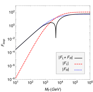
Figure 12: Loop functions, see eq. (12), that enter the neutrino mass, see eq. (11), generated by model 5, see figure 10. For this plot, the masses of $S_{1}$ and $S_{2}$ are taken to be $1$ TeV, while both fermion masses $M_{F_{1}}=M_{F_{2}}=M_{F}$.

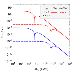
Figure 13: The neutrino mass scale for model 5 in figure 10, for some example choices of parameters. See text for details.

In figure 13 we show some examples for the neutrino mass scale for specific but arbitrary choices of parameters. Taking all the masses of the new scalars equal for simplicity, i.e. $m_{S_{1}}=m_{S_{2}}=m_{S}$, for masses of $\mathcal{O}(1)$ TeV Yukawas around ${\cal O}(0.5)$ are needed to generate the atmospheric scale. The difference, compared to the previous case of model 1, arises from the fact that the loop integral in model 5 contains one extra propagator compared to model 1, as well as one extra Yukawa coupling. Thus, the neutrino mass scales differently in model 5. The dependence on the masses is again easily understood, considering that for model 5 one has:

$$M_{\nu}\sim\mu_{S}m_{b}^{2}\left(\frac{M_{F}^{2}}{\Lambda^{4}}+\frac{1}{\Lambda^{2}}\right).$$ (15)

For $M_{F}\ll m_{S}$ one has a plateau whose height scales as $1/\Lambda^{2}$, instead of $1/\Lambda$ as in model 1, see eq. (15), while for large fermion masses both models have the same behaviour.

It is worth mentioning that model 5 contains an extra mass scale, i.e. the coupling $\mu_{S}$ in eq. (3.2). In fig. 13 we have chose $\mu_{S}=m_{S}$. Increasing its value will smoothen the differences between both models, making it possible to reach the measured neutrino mass scale with smaller Yukawas couplings. On the other hand, the need of at least one neutrino mass of the order of $0.05$ eV can be interpreted as a lower limit on this parameter.

We have chosen to discuss models 1 and 5 in more detail because they span the typical range of three-loop neutrino mass models. By direct inspection of the genuine diagrams, listed in figure 7, it can be seen that every integral contains 7 or 8 propagators, leading to the same behaviour as in either model 1 or model 5, respectively, in the limit of large masses. For small scalar and fermion masses, the scale of $M_{\nu}$ depends on the numerator of the integral, i.e. the number of fermions inside the loop along with the chiral structure of each vertex, as well as the presence of SM mass insertions.

Finally, we should point out that obviously any realistic neutrino mass model should be able to reproduce all neutrino oscillation data, i.e. the two neutrino mass squared differences along with three neutrino mixing angles and phases. The aim of our simplified examples was to show how the neutrino mass scales in typical 3-loop models; it was not to make a thorough neutrino flavour fit. However, going beyond the simplified scenario where there is just one non-zero charged lepton (or down-quark) mass the neutrino mass matrices given in (5) and (11) have rank-2. This makes it possible to fit normal or inverted hierarchical neutrino spectra, including a correct fit for angles and phases, in both model 1 and model 5. In order to fit a degenerate neutrino spectrum, a rank-3 neutrino mass matrix is needed. This can be achieved easily in model 5 just by adding extra copies of the new fields, for instance having two copies of $F_{1}$ and $F_{2}$. However, fitting a degenerate spectrum is not possible for the case of model 1, disregarding the number of copies of the fields. This is due to the antisymmetry of the Yukawa $Y_{1}$. Again, as with the overall mass scale, our two example models represent the two typical kind of models, that can be found at 3-loop order.

4 Conclusions

In this paper we have discussed the complete decomposition of the Weinberg operator at 3-loop order. Our analysis concentrates on finding those topologies and diagrams that can give the dominant contribution to the neutrino mass matrix, without the use of additional symmetries beyond those of the standard model. We call such topologies/diagrams genuine. We considered models with scalars and fermions only.

The requirement of “genuineness” eliminates the large majority of possible topologies: From more than four thousands, there are only 73 topologies which satisfy this criteria. We have discussed how to identify these cases and we listed them in appendix A. Those 73 genuine topologies were sub-divided into two classes: Normal ones (44 topologies) and special ones (29 topologies). While the former can be found systematically by our selection criteria, the latter topologies form an exception to our general rules, as explained in detail in section 2 and in the appendix A. This exception is related to the fact that usually, if any three fields (or four scalars) can interact through a loop, then they can also do so through a renormalizable local interaction. However, for special combinations of fields this is is not true: for example, the Higgs-Higgs-singlet local interaction is null, but a loop with these 3 external scalars does not need to have a zero amplitude.

The 44 topologies we have found are associated to a total of 228 diagrams in the electro-weak basis, from which one can get 3-loop leading order neutrino masses contributions. Going to the mass eigenstate basis, this list is reduced to only 18 diagrams (they are shown in figure 7). To these normal genuine diagrams one has to add 146 special ones , in the electroweak basis, which give another 12 mass eigenstate diagrams (see figure 8) We have also discussed how all those diagrams can be calculated with only five master integrals which where analysed in the literature previously [53]. We give them in appendix C, where we also show how the loop integrals for specific neutrino mass models can be constructed with two examples.

We have then also shown in section 3, how our general results can be easily used to build genuine 3-loop neutrino mass models. A few examples are briefly mentioned, and for two of them we have calculated the neutrino mass scale in more detail. This allows us to estimate the typical parameter range (couplings and masses), for which these 3-loop models can explain the measured neutrino oscillation data. We find that dimension 5 3-loop models will give a good fit to data if the new particles have masses roughly in the range $1-10^{3}$ TeV. Such a low scale is partially testable at current and future colliders, as well as in experiments searching for lepton flavour violation. Thus, 3-loop models are interesting constructions, since they are experimentally testable. We hope that model builders will find our results useful.

Acknowledgements

This work was supported by the Spanish grants FPA2017-85216-P and SEV-2014-0398 (AEI/FEDER, UE), Spanish consolider project MultiDark FPA2017-90566-REDC, FPU15/03158 (MECD) and PROMETEOII/2018/165 (Generalitat Valenciana). R.F. also acknowledges the financial support from the Grant Agency of the Czech Republic, (GAČR), contract nr. 17-04902S, as well as from the grant Juan de la Cierva-formación FJCI-2014-21651 (from Spain).

Appendix A List of genuine topologies

In this work we are interested in those scenarios where the dominant contribution to neutrino masses arises from a 3-loop realization of the Weinberg operator. As explained in the main text, genuine neutrino mass diagrams must descend from one of the 44 topologies shown in figure 14, otherwise it is not possible to forbid lower order contributions, independently of the assignment of fermions and scalars to the lines.

Figure 14: List of topologies associated to normal genuine diagrams. We refer to them in the text as $T_{i}$ with $i=1,\cdots,44$.

However, the procedure used to identify these 44 normal genuine topologies admits a loophole: in the presence of very special fields, it is possible to generate 3-loop neutrino masses diagrams with other topologies, with no lower order contributions appearing. In figure 15 we show these 29 special genuine topologies.

Figure 15: List of topologies associated to special genuine diagrams ($T_{i}$ with $i=45,\cdots,73$). The topologies are ordered according to specific field content needed in order to be considered as genuine. See the text for details.

Consider topology 54: there is only one way of making a fermion chain connecting the two external $L$’s hence there is a single diagram to be considered (see figure 16). One can identify in it a 2-loop subdiagram with 4 external scalar lines, shown in red in the middle of figure 16. Two of the external scalars are the Higgs fields of the Weinberg operator, while the others ($S$ and $S^{\prime}$) are unknown a priori, hence the subdiagram is associated to the operator $HHSS^{\prime}$. This means that, for most assignments of quantum numbers to the internal fields, one can write down such an interaction directly in a renormalizable Lagrangian, in which case neutrino masses can be generated via the 1-loop diagram shown in figure 16 on the right.

Figure 16: Topology 54 has only one diagram associated to it (shown here inside the box on the left). This diagram is only genuine under special conditions, in particular the two scalars interacting with the fermion line ($S$ and $S^{\prime}$) must be a Higgs $H$ and a scalar $\phi_{D}\equiv\left(\boldsymbol{1},\boldsymbol{2},-3/2\right)$.

However, strictly speaking the 2-loop subdiagram generates the non-local operator $H(x_{1})H(x_{2})S(x_{3})S^{\prime}(x_{4})$ which we may rewrite as

$$H\left(x_{1}\right)H\left(x_{2}\right)S\left(x_{3}\right)S^{\prime}\left(x_{4}\right)=H\left(x\right)H\left(x\right)S\left(x\right)S^{\prime}\left(x\right)+\sum_{n}c_{n}\frac{\partial^{2n}}{\Lambda^{2n}}H\left(x\right)H\left(x\right)S\left(x\right)S^{\prime}\left(x\right)\,,$$ (16)

where $x$ is some space-time point close to the $x_{i}$, $\Lambda$ is some mass scale and the $c_{n}$ are adimensional parameters. If $H(x)H(x)S(x)S^{\prime}(x)$ is nullified, the 1-loop neutrino mass depicted in figure 15 will not exist. Keeping in mind that in the Weinberg operator the two Higgs doublets contract as an $SU(2)$ triplet, there is only one possibility of avoiding a renormalizable $HHSS^{\prime}$ interaction: setting $S=H$ and $S^{\prime}=\phi_{D}\equiv\left(\boldsymbol{1},\boldsymbol{2},-3/2\right)$, or vice-versa. With this very special setup, the 3-loop diagram in figure 16 is genuine, and that is why the corresponding topology is included in figure 15.

As a more involved example, we will now discuss topology 71, for which there is a single genuine diagram, shown in figure 17. In this same figure, we indicate in red two subdiagrams (with 3 and 4 external lines) which should not be shrinkable to point interactions, otherwise the diagram becomes non-genuine. In particular, the internal scalars must be such that the local operators $HSS^{\prime}$ and $HS^{\prime}S^{\prime\prime}S^{\prime\prime\prime}$ are zero, while still allowing their non-local counterparts.

Figure 17: Topology 71 has one genuine diagram, shown here. The quantum numbers of the scalars must be special, otherwise one could build the Weinberg operator from a 1- or 2-loop diagram. In particular, this scenario is avoided only if $S=\phi_{S}\equiv\left(\boldsymbol{1},\boldsymbol{1},-1\right)$, $S^{\prime}=H$, $S^{\prime\prime}=\phi_{y}\equiv\left(\boldsymbol{1},\boldsymbol{1},y\right)$, and $S^{\prime\prime\prime}=\widetilde{\phi}_{y}\equiv\left(\boldsymbol{1},\boldsymbol{1},-1-y\right)$ for some hypercharge $y\neq 0,\pm 1,\pm 2$.

To nullify the first interaction, $HSS^{\prime}$, we must have either $S^{\prime}=S$, $S=H$ or $S^{\prime}=H$. But the first possibility ($HSS$) is no good, as there is no $SU(2)$ representation $\boldsymbol{R}$ such that $\boldsymbol{R}\times\boldsymbol{R}\times\boldsymbol{2}$ is gauge invariant. The second and third possibilities ($HHS$ and $HHS^{\prime}$), on the other hand, imply that either $S^{\prime}=\phi_{S}\equiv\left(\boldsymbol{1},\boldsymbol{1},-1\right)$ or $S=\phi_{S}$, respectively.

We consider now the other interaction, $HS^{\prime}S^{\prime\prime}S^{\prime\prime\prime}$, which also needs to be zero in its point-like realization. Given the two possible quantum number assignments for $S^{\prime}$, we might have $H\phi_{S}S^{\prime\prime}S^{\prime\prime\prime}$ or $HHS^{\prime\prime}S^{\prime\prime\prime}$. However, it is not complicated to check that $H\phi_{S}S^{\prime\prime}S^{\prime\prime\prime}$ would require either $S^{\prime\prime}$ or $S^{\prime\prime\prime}$ to be a gauge singlet $\left(\boldsymbol{1},\boldsymbol{1},0\right)$, so one could make a 2-loop realization of the Weinberg operator by removing this scalar line from the 3-loop diagram.

We then proceed with the only viable hypothesis — $HS^{\prime}S^{\prime\prime}S^{\prime\prime\prime}=HHS^{\prime\prime}S^{\prime\prime\prime}$. Again, we are faced with two scenarios: (a) one of the undetermined scalars ($S^{\prime\prime}$ and $S^{\prime\prime\prime}$) is equal to $H$, or (b) both $S^{\prime\prime}$ and $S^{\prime\prime\prime}$ are different from $H$. Scenario (a) implies that $\left(S^{\prime\prime},S^{\prime\prime\prime}\right)=\left(H,\phi_{D}\right)$, while scenario (b) leads to $S^{\prime\prime}=\phi_{y}\equiv\left(\boldsymbol{1},\boldsymbol{1},y\right)$, and $S^{\prime\prime\prime}=\widetilde{\phi}_{y}\equiv\left(\boldsymbol{1},\boldsymbol{1},-1-y\right)$ for some $y$. In the last case, both scalars must be $SU(2)$ singlets in order to ensure that the field product $S^{\prime\prime}S^{\prime\prime\prime}$ does not have a triplet component which would be responsible for coupling the two $H$’s symmetrically.

Taking into consideration everything said so far, it might then seem that there are two possibilities for topology 71 with the labelling as indicated on figure 17: $\left(S,S^{\prime},S^{\prime\prime},S^{\prime\prime\prime}\right)=\left(\phi_{S},H,H,\phi_{D}\right)$ and $\left(\phi_{S},H,\phi_{y},\widetilde{\phi}_{y}\right)$ (possibly switching the quantum number of $S^{\prime\prime}$ and $S^{\prime\prime\prime}$). However, a model with both the scalar $\phi_{S}$ and the scalar $\phi_{D}$ will inevitable generate the 2-loop diagram shown in figure 18, so the diagram in figure 17 is genuine only if $\left(S,S^{\prime},S^{\prime\prime},S^{\prime\prime\prime}\right)=\left(\phi_{S},H,\phi_{y},\widetilde{\phi}_{y}\right)$. It is worth mentioning that although the scalar loop with $\phi_{S}$ and $\phi_{D}$ in figure 18 seems to diverge, the loop is finite. This is because such special diagrams involve differences of two diagrams due to the $SU(2)_{L}$ contractions, removing the divergences. This is the same contractions that makes precisely $H(x)H(x)\phi_{S}(x)=0$.

For all the topologies in figure (15), we performed a similar analysis as in the previous examples, identifying the loop or loops at the diagram level that can exploit the loophole and, therefore, the specific field content needed for the diagram to be genuine. With this analysis, we classified the topologies in three groups such that all the diagrams generated by a certain topology require the same fields to be genuine. In figure (15), the first two rows of topologies (from topology 45 to 60) generate diagrams which contain one or two 4-point loop scalar vertices with at least one external higgs. The models descending from these topologies necessarily have the fields $\phi_{y}$, $\widetilde{\phi}_{y}$ and/or $\phi_{D}$ in order to be genuine. Topologies 61 to 70 generate diagrams with one 3-point internal loop, i.e. with no leg being a external leptons or Higgs. This can be either a 3-point scalar or fermion-fermion-scalar vertex. Note that in both cases the tree level should be zero, so one cannot have more than one copy of these fermions or scalars. Finally, the diagrams coming from the last three topologies 71, 72 and 73, contain at least one reducible loop with two scalars and an external higgs. In principle, one can avoid the corresponding 2-loop diagram with the recipe described in figure (17), thus making the topology genuine. Nevertheless, we mention that this diagram alone generates models which are not able fit neutrino data as they contain a structure identical to the simplest realization of the Zee model [7].

Figure 18: Two loop diagram which can be built in a model with the scalar fields $\phi_{S}\equiv\left(\boldsymbol{1},\boldsymbol{1},-1\right)$ and $\phi_{D}\equiv\left(\boldsymbol{1},\boldsymbol{2},-3/2\right)$. Note that because $H(x)H(x)\phi_{S}(x)=0$, it is not possible to remove the bottom loop in the diagram.

Just like the two example above, many of the 29 special topologies in figure 15 admit only 1 valid diagram, with specific quantum numbers assigned to some of the internal lines. Indeed, there is a total of 80 diagrams associated to these 29 topologies, which are distributed as follows (for topologies 45 to 73): 1, 1, 1, 1, 2, 3, 1, 1, 1, 1, 1, 4, 2, 2, 4, 2, 20, 18, 1, 1, 1, 1, 2, 3, 1, 1, 1, 1, 1. The complete list of diagrams can be found in [51].

Appendix B Relation between incompressible loops and genuineness of a diagram

We have mentioned in section 2 that those diagrams for which it is possible to compress one or more loops into a renormalizable vertex $v$ are not genuine, as one can then use the interaction $v$ to construct a similar diagram with less loops. In other words,

$$\textrm{loop compressibility }\Rightarrow\textrm{non-genuineness}\,.$$ (17)

Obviously, this is equivalent to the statement that genuine diagrams have incompressible loops ($\textrm{genuineness}\Rightarrow\textrm{loop incompressibility}$). However, this is not the same as

$$\textrm{loop incompressibility }\Rightarrow\textrm{genuineness}$$ (18)

and yet it was stated before that we expect this to be true. Indeed, our analysis relies on this important assumption, so in this appendix we discuss why we believe it to be true. We think that the argument presented here is compelling, but we stop short of calling it a proof.

First, consider the following intuitive/informal explanation for the implication (18). For particular assignments of quantum numbers to the internal lines of a diagram, there might be extra interactions between some of the diagram’s fields which are completely unrelated to the interactions used in the diagram. If that is the case, it might be possible to construct the Weinberg operator $LLHH$ with less loops by using the additional interactions. However, there will be a choice of quantum numbers of the internal lines such that this does not happen: no extra “non-trivial interactions” (see below) between the fields is possible, hence the operator $LLHH$ cannot be realized by a simpler diagram, with less loops.

In order to formalize this idea, consider only the abelian $U(1)_{Y}$ symmetry. In a $n$-loop diagram where the hypercharge of the external particles is fixed, the hypercharges $y_{i}$ of the internal lines depend on $n$ free numbers $\alpha_{j}$. More specifically, the $y_{i}$ are linear functions of these $n$ parameters:

$$y_{i}=c_{0}^{i}+\sum_{j=1}^{n}c_{j}^{i}\alpha_{j}\,,$$ (19)

where the $c_{0}^{i}$ and $c_{j}^{i}$ are numbers which depend on the hypercharge of the external particles and on the topology. Figure 19 shows an example where $y_{6}=y_{7}=1$ by choice, and $y_{1}=\alpha_{1}$, $y_{2}=1+\alpha_{1}$, $y_{3}=\alpha_{2}$, $y_{4}=-1+\alpha_{2}$, $y_{5}=1+\alpha_{1}-\alpha_{2}$ .

Figure 19: Two loop diagram with oriented lines $\ell_{i}$ and vertices $v_{j}$. The hypercharge of each line is indicated as a function of two free numbers: $\alpha_{1}$ and $\alpha_{2}$. The hypercharge of the external lines was fixed to 1 in this example.

A crucial question is then the following: what is the full list of interactions between the fields used in the diagram? From the point of view of the $U(1)_{Y}$ symmetry, any hypothetical interaction beyond those used in the diagram will either be (a) forbidden, (b) allowed for particular values of the $\alpha_{j}$ or (c) allowed for all values of the $\alpha_{j}$. Referring to figure (19), $\ell_{3}\ell_{4}^{*}$, $\ell_{1}\ell_{2}\ell_{3}$ and $\ell_{1}^{*}\ell_{2}\ell_{7}^{*}$ (respectively) are examples of each of these interactions. We will only be interested in those interaction of type (c) because we can choose the $\alpha_{j}$ in order to build a model where all interactions of type (a) and (b) are forbidden.

For the rest of this discussion, it is important to keep in mind that the $U(1)_{Y}$ symmetry is blind to combinations of a field and its conjugate, $\ell_{i}\ell_{i}^{*}$, hence one can add/remove them at will from any allowed vertex. Now, note that the hypercharges $y_{i}$ in equation (19) are the most general solutions to a linear system of equations

$$\sum_{j}C_{ij}y_{j}=0\,,$$ (20)

where the rows of the matrix $C$ represent each vertex, and its columns stand for each line in the diagram: if line number $j$ enters(leaves) vertex $i$, then $C_{ij}=1$($-1$), otherwise this entry is null. For the example in figure 19 we would have the following matrix:

$$C=\left(\begin{array}[]{ccccccc}-1&0&0&1&1&0&0\\ 0&1&-1&0&-1&0&0\\ 0&0&1&-1&0&0&-1\\ 1&-1&0&0&0&1&0\end{array}\right)\,.$$ (21)

For each external line in the diagram, since its hypercharge is fixed, one must add that constraint as well.

The important point is that any new vertex would correspond to adding a new row to matrix $C$. This operation will not change the solution space if and only if the new row is a linear combination of the existing rows (the solutions of $C\cdot y=0$ and $C^{\prime}\cdot y=0$ are the same only if the lines of $C^{\prime}$ are linear combinations of those of $C$). Additions and subtractions of rows of $C$ translates into making new vertices $v$ which are the product of existing ones (addition) or its conjugates (subtraction): $v=v_{i}^{(*)}v_{j}^{(*)}v_{k}^{(*)}\cdots$. The vertices obtained in this way account for all unavoidable interactions (considering the $U(1)_{Y}$ group only).

For example, there are vertices $v_{1}=\ell_{1}^{*}\ell_{4}\ell_{5}$ and $v_{2}=\ell_{2}\ell_{3}^{*}\ell_{5}^{*}$ and in figure 19, so the interactions $v_{2}v_{2}=\ell_{2}\ell_{2}\ell_{3}^{*}\ell_{3}^{*}\ell_{5}^{*}\ell_{5}^{*}$ or $v_{1}^{*}v_{2}=\ell_{1}\ell_{2}\ell_{3}^{*}\ell_{4}^{*}\ell_{5}^{*}\ell_{5}^{*}$ cannot be forbidden by any choice of $\alpha_{1},\alpha_{2}$. Nevertheless, these are non-renormalizable interactions: to reduce the number of fields in these new interactions, one can only use the fact that combinations of the form $\ell_{i}\ell_{i}^{*}$ are irrelevant for the $U(1)_{Y}$ symmetry, hence for example $v_{1}v_{2}=\ell_{1}^{*}\ell_{2}\ell_{3}^{*}\ell_{4}$ (modulo $\ell_{5}\ell_{5}^{*}$). Graphically, it is very easy to follow what is happening: we remove the line $\ell_{5}$ connecting the vertices $v_{1}$ and $v_{2}$, condensing them into a quartic interaction. Applying this process repeatedly for the internal lines $\ell_{3}$, $\ell_{4}$ and $\ell_{5}$, one generates the new interaction $\ell_{1}^{*}\ell_{2}\ell_{7}^{*}$ ($=v_{1}v_{2}v_{3}$ modulo $\ell_{i}\ell_{i}^{*}$’s) which graphically is obtained by collapsing the lower loop of the diagram into a point.

Another interesting example are those cases where the same field appears in more than one line in the diagram. For the present discussion what is important are those situations where this is unavoidable, rather than just possible. According to the previous discussion, two lines $\ell$ and $\ell^{\prime}$ must have the same hypercharge (and therefore potentially represent the same field) if and only if the bilinear interaction $\ell^{*}\ell^{\prime}$ is unavoidable, i.e. one must be able to merge various of the diagram vertices into such interaction. Lines $\ell_{6}$ and $\ell_{7}$ in figure 19 constitute an example of such a scenario (they are external lines, hence their hypercharge was fixed to 1 in our example, but even if they were internal lines of a bigger diagram, $U(1)_{Y}$ invariance could not forbid the coupling $\ell_{6}^{*}\ell_{7}$).

In summary,

1. For a $n$-loop diagram, the hypercharge of the internal lines depends on $n$ free numbers $\alpha_{i}$.

2. The only interactions between the various lines which cannot be forbidden for any choice of $\alpha_{i}$ (the $U(1)_{Y}$ unavoidable interactions) are those for which the sum of hypercharges is identically 0, i.e. $0+0\alpha_{1}+0\alpha_{2}+\cdots 0\alpha_{n}$. (Only a subset of these interactions are truly unavoidable as one should take into account the full Standard Model symmetry, as well as Lorentz invariance.)

3. The full list of $U(1)_{Y}$ unavoidable interactions can be obtained by merging together the diagram vertices (and/or their conjugates). In this merging process, $\left(\textrm{line X}\right)\left(\textrm{line X}\right)^{*}$ combinations can be added or removed.

4. Most of these unavoidable interactions are non-renormalizable. Renormalizable new vertices can be formed only if there are those removable $\left(\textrm{line X}\right)\left(\textrm{line X}\right)^{*}$ combinations mentioned earlier, otherwise by merging vertices the number of lines constantly increasing. Graphically, this corresponds to coalescing adjacent vertices in the diagram, and removing the line(s) connecting them.

There are 4 external lines ($LLHH$) indirectly connected to each other through a web of vertices and internal lines. The unavoidable alternative ways of connecting these 4 lines must be through an alternative web of unavoidable vertices. Graphically, this new web of lines and vertices must be obtained from the original one by the vertex-merging process described above. So, if it is not possible to remove one or more loops from a diagram by collapsing them into a point, the diagram is genuine.

Appendix C Master integrals for 3-loop neutrino masses

In this appendix, we give the minimal set of integrals that span the complete list of possible genuine models. In principle, starting from the list of 30 genuine diagrams in the mass eigenbasis (see fig. 7 and 8), one should obtain at least 30 integrals assigning momenta to the fields. This initial set, however, can be further reduced applying the results previously used in 2-loop calculations in [12, 56], both based on [57], and 3-loop integrals in [58, 53]. Here, we are going to summarize the results in these papers which we need.

Using the notation of [53], we can write:

$$\mathbf{T}^{(n_{1},n_{2},n_{3},n_{4},n_{5},n_{6})}(x_{1},x_{2},x_{3},x_{4},x_{5},x_{6})=\iiint\limits_{(k_{1},k_{2},k_{3})}\frac{1}{[k_{1}^{2}-x_{1}]^{n_{1}}[k_{2}^{2}-x_{2}]^{n_{2}}[k_{3}^{2}-x_{3}]^{n_{3}}[(k_{1}-k_{2})^{2}-x_{4}]^{n_{4}}[(k_{2}-k_{3})^{2}-x_{5}]^{n_{5}}[(k_{3}-k_{1})^{2}-x_{6}]^{n_{6}}}$$ (22)

Here we have used the abbreviation given in eq. (8) and the powers of the propagators $n_{i}$ can be any integer number. Note that the integral is invariant under the interchange of pairs $(n_{i},x_{i})$ and moreover, satisfies the nine identities obtained by integration by parts [59],

$$0=\iiint\limits_{(k_{1},k_{2},k_{3})}\frac{\partial}{\partial k_{i}^{\mu}}\left[k_{j}^{\mu}\mathbf{X}\right],$$ (23)

for $i,j=1,2,3$, with $\mathbf{X}$ equal to any product of propagators of the form shown in eq. (22). One can find very useful identities for this kind of integrals, such as:

$$\frac{3}{2}d+\sum\limits_{j=1}^{6}(x_{j}\mathbf{j}^{+}-1)n_{j}=0.$$ (24)

Here $d$ is the dimension of the momentum integration in dimensional regularization and $\mathbf{j}^{\pm}$ is short-hand notation for the following operator:

$$\mathbf{j}^{\pm}\mathbf{T}^{(...,n_{j},...)}=\mathbf{T}^{(...,n_{j}\pm 1,...)}.$$ (25)

By repeated application of the identities (23), any of the 3-loop integrals $\mathbf{T}$ can be reduced to a linear combination of five master integrals [53]:

$$\mathbf{H}(x_{1},x_{2},x_{3},x_{4},x_{5},x_{6}) =\mathbf{T}^{(1,1,1,1,1,1)}(x_{1},x_{2},x_{3},x_{4},x_{5},x_{6})$$

$$\mathbf{G}(x_{3},x_{1},x_{6},x_{2},x_{5}) =\mathbf{T}^{(1,1,1,0,1,1)}(x_{1},x_{2},x_{3},x_{4},x_{5},x_{6})$$

$$\mathbf{F}(x_{1},x_{2},x_{5},x_{6}) =\mathbf{T}^{(2,1,0,0,1,1)}(x_{1},x_{2},x_{3},x_{4},x_{5},x_{6})$$ (26)

$$\mathbf{A}(x_{1})\mathbf{I}(x_{2},x_{3},x_{5}) =\mathbf{T}^{(1,1,1,0,1,0)}(x_{1},x_{2},x_{3},x_{4},x_{5},x_{6})$$

$$\mathbf{A}(x_{1})\mathbf{A}(x_{2})\mathbf{A}(x_{3}) =\mathbf{T}^{(1,1,1,0,0,0)}(x_{1},x_{2},x_{3},x_{4},x_{5},x_{6}).$$

where $\mathbf{A}$ is the standard one-loop Passarino-Veltman function [60] and $\mathbf{I}$ is a two-loop integral described in [57]. It is worth mentioning that analytical expressions exist for the well-known integrals $\mathbf{A}$ and $\mathbf{I}$, while for the three-loop ones ($\mathbf{F}$, $\mathbf{G}$, and $\mathbf{H}$) results are known only for particular cases (see [53] for details).

Particularizing to our case, starting from the 30 diagrams in figure 7 and 8, in the mass insertion approximation, and assigning momenta to the internal lines, one can find that the integrals have repeated propagators with equal momenta but different masses. One can prove that every 3-loop integral in figure 7 and 8 can be written in terms of the integrals in eq. (22). We note here that partial fractions can be used to reduce the number of propagators with common momenta [57]:

$$\mathbf{T}^{(\left\{n_{11},n_{12}\right\},n_{2},n_{3},n_{4},n_{5},n_{6})}(\left\{x_{11},x_{12}\right\} ,x_{2},x_{3},x_{4},x_{5},x_{6})=$$ (27)

$$\frac{1}{x_{11}-x_{12}}\Big{[} \mathbf{T}^{(\left\{n_{11},n_{12}-1\right\},n_{2},n_{3},n_{4},n_{5},n_{6})}(\left\{x_{11},x_{12}\right\},x_{2},x_{3},x_{4},x_{5},x_{6})$$

$$- \mathbf{T}^{(\left\{n_{11}-1,n_{12}\right\},n_{2},n_{3},n_{4},n_{5},n_{6})}(\left\{x_{11},x_{12}\right\},x_{2},x_{3},x_{4},x_{5},x_{6})\Big{]},$$

where $\mathbf{T}^{(\left\{n_{11},n_{12}\right\},n_{2},n_{3},n_{4},n_{5},n_{6})}(\left\{x_{11},x_{12}\right\},x_{2},x_{3},x_{4},x_{5},x_{6})$ is the same as $\mathbf{T}$ without the braces, but with an extra propagator $[k_{1}^{2}-x_{12}]^{n_{12}}$.

On the other hand, some integrals with a non-trivial integrand numerator can be further simplificatied using the $p^{2}$-decomposition, namely

$$\frac{p^{2}}{(k^{2}-x_{1})(p^{2}-x_{2})}=\frac{1}{(k^{2}-x_{1})}+\frac{x_{2}}{(k^{2}-x_{1})(p^{2}-x_{2})}.$$ (28)

To demonstrate how this procedure works in practice, we can take for instance the loop integral of model 1, given in eq. (6) of section 3. Applying the identity (27) twice to both propagators sharing $k_{1}$ and $k_{2}$ momenta, $F_{loop}\!\left(x_{1},x_{2}\right)$ can be directly decomposed in terms of a linear combination of $\mathbf{G}$’s:

$$F_{loop}\!\left(x_{1},x_{2}\right)=\frac{1}{x_{1}^{2}}\bigg{\{}\mathbf{G}(1,x_{1},x_{2},x_{1},x_{1})-\mathbf{G}(1,x_{1},x_{2},0,x_{1})-\mathbf{G}(1,0,x_{2},x_{1},x_{1})+\mathbf{G}(1,0,x_{2},0,x_{1})\bigg{\}}.$$ (29)

For model 5, the decomposition of the loop integral $F_{L}(x_{1},x_{2})$ in (12) is straightforward given the previous example. One only has to apply eq. (27) three times to obtain a linear combination of eight $\mathbf{G}$ integrals. Here we focus on the decomposition of $F_{R}(x_{1},x_{2})$, just to present an example of a integral with a non-trivial numerator. One should first notice that under the integral sign

$$\not{k_{3}}(\not{k_{2}}+\not{k_{3}})\longrightarrow k_{3}\cdot(k_{2}+k_{3})=\frac{1}{2}\left[(k_{2}+k_{3})^{2}-k_{2}^{2}+k_{3}^{2}\right].$$ (30)

It is clear that one should apply the $p^{2}$-decomposition in eq. (28) along with the partial fractions decomposition (27), as in the previous case, to get rid of the numerator and the repeated propagators. The full process of the decomposition is rather lengthy and cumbersome, so here we give just the final result.

$$F_{L}(x_{1},x_{2},x_{3},x_{4})=\frac{\sqrt{x_{1}x_{3}}}{x_{1}-x_{2}}\bigg{\{} \mathbf{G}(x_{1},1,x_{4},1,x_{3})-\mathbf{G}(x_{1},1,x_{4},0,x_{3})-\mathbf{G}(x_{1},0,x_{4},1,x_{3})+\mathbf{G}(x_{1},0,x_{4},0,x_{3})$$

$$- \mathbf{G}(x_{2},1,x_{4},1,x_{3})+\mathbf{G}(x_{2},1,x_{4},0,x_{3})+\mathbf{G}(x_{2},0,x_{4},1,x_{3})-\mathbf{G}(x_{2},0,x_{4},0,x_{3})\bigg{\}},$$ (31)

$$F_{R}(x_{1},x_{2},x_{3},x_{4})=\frac{1}{2}\frac{1}{x_{1}-x_{2}}\bigg{\{}(x_{1}+x_{3}-1) \Big{[}\mathbf{G}(x_{1},1,x_{4},1,x_{3})-\mathbf{G}(x_{1},0,x_{4},1,x_{3})\Big{]}$$

$$-(x_{1}+x_{3}) \Big{[}\mathbf{G}(x_{1},1,x_{4},0,x_{3})-\mathbf{G}(x_{1},0,x_{4},0,x_{3})\Big{]}$$

$$-(x_{2}+x_{3}-1) \Big{[}\mathbf{G}(x_{2},1,x_{4},1,x_{3})-\mathbf{G}(x_{2},0,x_{4},1,x_{3})\Big{]}$$

$$+(x_{2}+x_{3}) \Big{[}\mathbf{G}(x_{2},1,x_{4},0,x_{3})-\mathbf{G}(x_{2},0,x_{4},0,x_{3})\Big{]}$$

$$+\Big{[}\mathbf{A}(1)-\mathbf{A}(0)\Big{]} \Big{[}\mathbf{I}(x_{1},1,x_{4})-\mathbf{I}(x_{1},0,x_{4})-\mathbf{I}(x_{2},1,x_{4})+\mathbf{I}(x_{2},0,x_{4})\Big{]}\bigg{\}}.$$ (32)

One can check that the loop integral decompositions are still symmetric under the interchange of $x_{1}$ and $x_{2}$, as it was the case with the original integral definitions in eq. (12).

Erratum

The strategy used in our original publication to classify the 3-loop realizations of the Weinberg operator admits a loophole which was overlooked; it enlarges the set of genuine topologies. We have found that by means of this loophole, the 26 topologies depicted in figure 20 categorized as non-genuine in our original publication actually have to be classified as special genuine. Recall that special genuine topologies are those associated to neutrino mass diagrams which under normal circumstances can be redrawn with less loops, unless some particular quantum numbers are assigned to some of the particles in the internal lines. More specifically, these special diagrams contain fermion-fermion-scalar, $\left(\textrm{scalar}\right)^{3}$ and/or $\left(\textrm{scalar}\right)^{4}$ effective interactions generated through loops which cannot be compressed to a point, as is ordinarily the case. That is because these effective couplings involve derivatives of the fields, making them non-renormalizable, so there exist exceptional cases in which there is no corresponding tree level realization of the effective vertex.

For the special genuine topologies discussed in the paper, the existence of derivatives can be traced to the antisymmetric nature of some $SU(2)_{L}$ contractions, which makes some loop interactions non-compressible for appropriate choices of the quantum numbers of the diagram lines. However, when writing the paper we overlooked a second possible reason why such derivative terms might be unavoidable: fermion-fermion-scalar couplings may contain a derivative due to the chirality of the standard model fermions. In particular, two left-handed Weyl fermions $\psi$ and $\psi^{\prime}$ may interact with a scalar $S$ through a $\partial\psi^{\dagger}\psi^{\prime}S$ effective coupling (the number of derivatives can be higher, as long as it is an odd number). However, if $\psi$ is a vector-like field, its left-handed partner $\overline{\psi}$ has the same gauge quantum numbers as $\psi^{\dagger}$ (the conjugate of $\psi$) and opposite chirality, hence there is no symmetry forbidding the renormalizable interaction $\overline{\psi}\psi^{\prime}S$, with no derivatives. Using this coupling and a mass insertion $\overline{\psi}\psi$ one can then always generate $\partial\psi^{\dagger}\psi^{\prime}S$ without loops, as depicted in figure 21. However, if neither $\psi$ nor $\psi^{\prime}$ has a vector-like partner, this argument fails and the vertex $\partial\psi^{\dagger}\psi^{\prime}S$ may not be realizable at tree-level. Thus, if $\psi$ and $\psi^{\prime}$ are fixed to be Standard Model fermions, the loop might not be compressible and our general arguments fail. Let us discuss this with one particular example.

Figure 20: List of new topologies associated to special genuine diagrams. We follow the numbering of the paper and this list should be understood as a continuation of figure 15 in the Appendix A of the paper. See text for details.

Figure 21: Consider a loop induced coupling of the left-handed fermions $\psi$ and $\psi^{\prime}$ to a scalar $S$ as indicated on the left. Given the chirality of the fermions, the effective coupling is $\partial\psi^{\dagger}\psi^{\prime}S$. If $\psi$ has a vector-like partner $\overline{\psi}$ (which we may consider to be left-handed as well), then the tree-level coupling $\overline{\psi}\psi^{\prime}S$ exists, and together with a mass insertion $\overline{\psi}\psi$ it can be used to generate the effective interaction $\partial\psi^{\dagger}\psi^{\prime}S$ without loops (this is the leading order interaction; extra pairs of derivatives appear at higher order). This argument fails if both $\psi$ and $\psi^{\prime}$ are Standard Model fermions.

Take for instance topology 89 in figure 20 and one of its diagrams as an example (shown in figure 22). This diagram contains a one-loop realization of the vertex $\partial L\psi^{\dagger}S$, with $L$ the SM lepton doublet and $\psi$ and $S$ an arbitrary left-handed fermion and scalar, respectively. If $\psi$ is not a Standard Model fermion, it is necessary to add its vector-like partner $\overline{\psi}$ to the model, in order to generate a bare mass term $M\overline{\psi}\psi$. From the argument in figure 21, it is then possible to rewrite the diagram with one less loop. On the other hand, it might not be possible to do so if $\psi$ is a Standard Model fermion, in which case the diagram is genuine.

Note that, since this loophole to our general argument exists only for standard model fermions, the list of all possible genuine models generated from the diagram in figure 22 will be quite constrained, due to the limited number of choices of $\psi\in\{L,e^{c},Q,u^{c},d^{c}\}$.

In total, there are 125 genuine diagrams associated to the 26 topologies in figure 20. They yield 8 new diagrams in the mass basis, after electroweak symmetry breaking (see figure 23). The complete lists of topologies and diagrams are given in [51].

Figure 22: Example of a diagram with topology 89, containing a one-loop fermion-fermion-scalar effective interaction (in red). This loop is removable unless $\psi$ is a SM fermion.

Figure 23: List of new special genuine diagrams in the mass basis, i.e. with the external Higgs lines removed. The numbering follows that of figure 8 of the paper and should be understood as a continuation of that figure.

The newly re-classified topologies, see figure 20, and diagrams, figure 23, affect some numbers quoted in our original paper. In figure 24 we give the updated numbers for each type of topology and each type of diagram.

Figure 24: Corrected counting for topologies and diagrams.

References

- [1] S. Weinberg, Baryon and Lepton Nonconserving Processes, Phys. Rev. Lett. 43 (1979) 1566–1570.
- [2] P. Minkowski, at a rate of one out of muon decays?, Phys.Lett. B67 (1977) 421.
- [3] T. Yanagida, Horizontal symmetry and masses of neutrinos, Workshop on the baryon number of the Universe and unified theories, O. Sawada and A. Sugamoto, eds. (1979) 95.
- [4] R. N. Mohapatra and G. Senjanovic, Neutrino mass and spontaneous parity violation, Phys. Rev. Lett. 44 (1980) 912.
- [5] J. Schechter and J. Valle, Neutrino masses in theories, Phys. Rev. D22 (1980) 2227.
- [6] G. Anamiati et al., High-dimensional neutrino masses (2018), arXiv:1806.07264 [hep-ph].
- [7] A. Zee, A theory of lepton number violation, neutrino Majorana mass, and oscillation, Phys.Lett. B93 (1980) 389.
- [8] Y. Cai et al., From the trees to the forest: a review of radiative neutrino mass models, Front.in Phys. 5 (2017) 63, arXiv:1706.08524 [hep-ph].
- [9] Y. Farzan, S. Pascoli and M. A. Schmidt, Recipes and ingredients for neutrino mass at loop level, JHEP 03 (2013) 107, arXiv:1208.2732 [hep-ph].
- [10] E. Ma, Pathways to naturally small neutrino masses, Phys.Rev.Lett. 81 (1998) 1171–1174, arXiv:hep-ph/9805219 [hep-ph].
- [11] F. Bonnet, M. Hirsch, T. Ota and W. Winter, Systematic study of the Weinberg operator at one-loop order, JHEP 1207 (2012) 153, arXiv:1204.5862 [hep-ph].
- [12] D. Aristizabal Sierra, A. Degee, L. Dorame and M. Hirsch, Systematic classification of two-loop realizations of the Weinberg operator, JHEP 03 (2015) 040, arXiv:1411.7038 [hep-ph].
- [13] F. Bonnet, D. Hernandez, T. Ota and W. Winter, Neutrino masses from higher than effective operators, JHEP 0910 (2009) 076, arXiv:0907.3143 [hep-ph].
- [14] R. Cepedello, M. Hirsch and J. C. Helo, Loop neutrino masses from operator, JHEP 07 (2017) 079, arXiv:1705.01489 [hep-ph].
- [15] K. S. Babu, S. Nandi and Z. Tavartkiladze, New mechanism for neutrino mass generation and triply charged Higgs bosons at the LHC, Phys. Rev. D80 (2009) 071702, arXiv:0905.2710 [hep-ph].
- [16] K. S. Babu and C. N. Leung, Classification of effective neutrino mass operators, Nucl. Phys. B619 (2001) 667–689, arXiv:hep-ph/0106054 [hep-ph].
- [17] A. de Gouvea and J. Jenkins, A Survey of Lepton Number Violation Via Effective Operators, Phys. Rev. D77 (2008) 013008, arXiv:0708.1344 [hep-ph].
- [18] P. W. Angel, N. L. Rodd and R. R. Volkas, Origin of neutrino masses at the LHC: effective operators and their ultraviolet completions, Phys. Rev. D87 (2013) 7 073007, arXiv:1212.6111 [hep-ph].
- [19] L. M. Krauss, S. Nasri and M. Trodden, A model for neutrino masses and dark matter, Phys. Rev. D67 (2003) 085002, arXiv:hep-ph/0210389 [hep-ph].
- [20] K. Cheung and O. Seto, Phenomenology of TeV right-handed neutrino and the dark matter model, Phys. Rev. D69 (2004) 113009, arXiv:hep-ph/0403003 [hep-ph].
- [21] A. Ahriche, C.-S. Chen, K. L. McDonald and S. Nasri, Three-loop model of neutrino mass with dark matter, Phys. Rev. D90 (2014) 015024, arXiv:1404.2696 [hep-ph].
- [22] A. Ahriche, K. L. McDonald and S. Nasri, A Model of radiative neutrino mass: with or without dark matter, JHEP 10 (2014) 167, arXiv:1404.5917 [hep-ph].
- [23] C.-S. Chen, K. L. McDonald and S. Nasri, A class of three-loop models with neutrino mass and dark matter, Phys. Lett. B734 (2014) 388–393, arXiv:1404.6033 [hep-ph].
- [24] P.-H. Gu, From dark matter to neutrinoless double beta decay (2012), arXiv:1203.4165 [hep-ph].
- [25] T. Nomura, H. Okada and N. Okada, A Colored KNT neutrino model, Phys. Lett. B762 (2016) 409–414, arXiv:1608.02694 [hep-ph].
- [26] K. Cheung, T. Nomura and H. Okada, Three-loop neutrino mass model with a colored triplet scalar, Phys. Rev. D95 (2017) 1 015026, arXiv:1610.04986 [hep-ph].
- [27] H. Okada and K. Yagyu, Renormalizable model for neutrino mass, dark matter, muon and 750 GeV diphoton excess, Phys. Lett. B756 (2016) 337–344, arXiv:1601.05038 [hep-ph].
- [28] A. Ahriche, K. L. McDonald and S. Nasri, A radiative model for the weak scale and neutrino mass via dark matter, JHEP 02 (2016) 038, arXiv:1508.02607 [hep-ph].
- [29] A. Ahriche, K. L. McDonald and S. Nasri, Scalar sector phenomenology of three-loop radiative neutrino mMass models, Phys. Rev. D92 (2015) 9 095020, arXiv:1508.05881 [hep-ph].
- [30] A. Ahriche, K. L. McDonald and S. Nasri, Three-loop neutrino mass models at colliders, in Proceedings, 50th Rencontres de Moriond Electroweak Interactions and Unified Theories: La Thuile, Italy, March 14-21, 2015 (2015) pages 285–290, arXiv:1505.04320 [hep-ph], URL http://inspirehep.net/record/1370679/files/arXiv:1505.04320.pdf.
- [31] A. Ahriche, S. Nasri and R. Soualah, Radiative neutrino mass model at the linear collider, Phys. Rev. D89 (2014) 9 095010, arXiv:1403.5694 [hep-ph].
- [32] A. Ahriche, K. L. McDonald, S. Nasri and T. Toma, A model of neutrino mass and dark matter with an accidental symmetry, Phys. Lett. B746 (2015) 430–435, arXiv:1504.05755 [hep-ph].
- [33] C. Hati, G. Kumar, J. Orloff and A. M. Teixeira, Reconciling -decay anomalies with neutrino masses, dark matter and constraints from flavour violation (2018), arXiv:1806.10146 [hep-ph].
- [34] M. Aoki, S. Kanemura and O. Seto, Neutrino mass, dark matter and baryon asymmetry via TeV-scale physics without fine-tuning, Phys. Rev. Lett. 102 (2009) 051805, arXiv:0807.0361 [hep-ph].
- [35] M. Aoki, S. Kanemura and O. Seto, A model of TeV scale physics for neutrino mass, dark matter and baryon asymmetry and its phenomenology, Phys. Rev. D80 (2009) 033007, arXiv:0904.3829 [hep-ph].
- [36] M. Aoki, S. Kanemura and O. Seto, ILC phenomenology in a TeV scale radiative seesaw model for neutrino mass, dark matter and baryon asymmetry, in 8th General Meeting of the ILC Physics Subgroup Tsukuba, Japan, January 21, 2009 (2010) arXiv:1008.2407 [hep-ph], URL http://inspirehep.net/record/865435/files/arXiv:1008.2407.pdf.
- [37] M. Aoki, S. Kanemura and K. Yagyu, Triviality and vacuum stability bounds in the three-loop neutrino mass model, Phys. Rev. D83 (2011) 075016, arXiv:1102.3412 [hep-ph].
- [38] H. Okada and K. Yagyu, Three-loop neutrino mass model with doubly charged particles from isodoublets, Phys. Rev. D93 (2016) 1 013004, arXiv:1508.01046 [hep-ph].
- [39] P. Ko, T. Nomura, H. Okada and Y. Orikasa, Confronting a new three-loop seesaw model with the 750 GeV diphoton excess, Phys. Rev. D94 (2016) 1 013009, arXiv:1602.07214 [hep-ph].
- [40] P.-H. Gu, High-scale leptogenesis with three-loop neutrino mass generation and dark matter, JHEP 04 (2017) 159, arXiv:1611.03256 [hep-ph].
- [41] P. Culjak, K. Kumericki and I. Picek, Scotogenic RMDM at three-loop level, Phys. Lett. B744 (2015) 237–243, arXiv:1502.07887 [hep-ph].
- [42] H. Hatanaka, K. Nishiwaki, H. Okada and Y. Orikasa, A three-loop neutrino model with global Symmetry, Nucl. Phys. B894 (2015) 268–283, arXiv:1412.8664 [hep-ph].
- [43] T. P. Cheng and L.-F. Li, Neutrino masses, mixings and oscillations in models of electroweak interactions, Phys. Rev. D22 (1980) 2860.
- [44] A. Zee, Quantum numbers of Majorana neutrino masses, Nucl. Phys. B264 (1986) 99–110.
- [45] K. S. Babu, Model of “calculable” Majorana neutrino masses, Phys. Lett. B203 (1988) 132–136.
- [46] K. Nishiwaki, H. Okada and Y. Orikasa, Three loop neutrino model with isolated , Phys. Rev. D92 (2015) 9 093013, arXiv:1507.02412 [hep-ph].
- [47] B. Dutta, S. Ghosh, I. Gogoladze and T. Li, Three-loop neutrino masses via new massive gauge bosons from GUT (2018), arXiv:1805.01866 [hep-ph].
- [48] K. Cheung, T. Nomura and H. Okada, A three-loop neutrino model with leptoquark tTriplet scalars, Phys. Lett. B768 (2017) 359–364, arXiv:1701.01080 [hep-ph].
- [49] M. Gustafsson, J. M. No and M. A. Rivera, Predictive model for radiatively induced neutrino masses and mixings with dark matter, Phys. Rev. Lett. 110 (2013) 21 211802, [Erratum: Phys. Rev. Lett.112,no.25,259902(2014)], arXiv:1212.4806 [hep-ph].
- [50] M. Gustafsson, J. M. No and M. A. Rivera, Radiative neutrino mass generation linked to neutrino mixing and -decay predictions, Phys. Rev. D90 (2014) 1 013012, arXiv:1402.0515 [hep-ph].
- [51] Systematic classification of three-loop realizations of the Weinberg operator: Extra data, See supplementary material, available also at http://renatofonseca.net/3loop-Weinberg-operator.php, accessed: 05/06/2019.
- [52] R. C. Read, A survey of graph generation techniques, in K. L. McAvaney (editor), Combinatorial Mathematics VIII, Springer Berlin Heidelberg, Berlin, Heidelberg, ISBN 978-3-540-38792-3 (1981) pages 77–89.
- [53] S. P. Martin and D. G. Robertson, Evaluation of the general 3-loop vacuum Feynman integral, Phys. Rev. D95 (2017) 1 016008, arXiv:1610.07720 [hep-ph].
- [54] S. Borowka et al., pySecDec: a toolbox for the numerical evaluation of multi-scale integrals, Comput. Phys. Commun. 222 (2018) 313–326, arXiv:1703.09692 [hep-ph].
- [55] P. Langacker and G. Steigman, Requiem for an FCHAMP? Fractionally CHArged, Massive Particle, Phys. Rev. D84 (2011) 065040, arXiv:1107.3131 [hep-ph].
- [56] K. L. McDonald and B. H. J. McKellar, Evaluating the two loop diagram responsible for neutrino mass in Babu’s model (2003), arXiv:hep-ph/0309270 [hep-ph].
- [57] J. van der Bij and M. J. G. Veltman, Two loop large Higgs mass correction to the -parameter, Nucl. Phys. B231 (1984) 205–234.
- [58] A. Freitas, Three-loop vacuum integrals with arbitrary masses, JHEP 11 (2016) 145, arXiv:1609.09159 [hep-ph].
- [59] K. G. Chetyrkin and F. V. Tkachov, Integration by parts: the algorithm to calculate -functions in 4 loops, Nucl. Phys. B192 (1981) 159–204.
- [60] G. Passarino and M. J. G. Veltman, One loop corrections for annihilation into in the Weinberg model, Nucl. Phys. B160 (1979) 151–207.