Mixing of the Square Plaquette Model on a Critical Length Scale

Abstract

Plaquette models are short range ferromagnetic spin models that play a key role in the dynamic facilitation approach to the liquid glass transition. In this paper we study the dynamics of the square plaquette model at the smallest of the three critical length scales discovered in [Chleboun2017]. Our main results are estimates of the spectral gap and mixing time for two natural boundary conditions. As a consequence, we observe that these time scales depend heavily on the boundary condition in this scaling regime.

1 Introduction

In this paper we consider the dynamics of the square plaquette model (SPM) at low temperature. Spin plaquette models were originally associated with glassy behaviour in [Garrahan2002b, Newman1999], where it was argued that they have more physically-realistic dynamics and thermodynamic properties than kinetically-constrained models, while remaining mathematically tractable. These models have also recently been generalised to quantum systems, called fracton models, which show extremely similar relaxation behaviour [Chamon2005, Nandkishore2018]. Plaquette models are defined over an integer lattice $\Lambda\subseteq{\mathbb{Z}}^{d}$, and configurations of the plaquette model correspond to $\pm 1$-valued labellings of the lattice $\Lambda$. Every configuration of the SPM has an associated energy given by certain short range ferromagnetic interactions that are defined in terms of the plaquettes, a collection of subsets of ${\mathbb{Z}}^{2}$ denoted by $\mathcal{P}$.

More formally, plaquette models are families of probability distributions with state space $\{-1,+1\}^{\Lambda}$. Every configuration $\sigma\in\{-1,+1\}^{\Lambda}$ has an associated energy value, given by the Hamiltonian

$$H(\sigma)=-\frac{1}{2}\sum_{P\in\mathcal{P}}\prod_{x\in P}\sigma_{x}\,.$$

For any fixed inverse-temperature $\beta>0$, we then associate to this Hamiltonian the probability distribution $\pi_{\Lambda}^{\beta}$ on $\{-1,1\}^{\Lambda}$ given by $\pi_{\Lambda}^{\beta}(\sigma)\propto\textrm{exp}(-\beta H_{\Lambda}(\sigma))$. In the case of the SPM, we always take $\Lambda\subset{\mathbb{Z}}^{2}$ and the plaquettes are exactly the collection of unit squares contained in $\Lambda$. There are several natural Markov chains associated with these probability distributions, many of which have very similar behaviour. In this paper we study the most popular of these Markov chains, the continuous-time single-spin Glauber dynamics (also known as the Gibbs sampler). Roughly speaking, this Markov chain evolves from a configuration $\sigma$ by choosing a random site $x\in\Lambda$ at unit rate and then updating the value $\sigma(x)$ conditional on $\{\sigma(y)\}_{y\in\Lambda\backslash\{x\}}$ according to the measure $\pi_{\Lambda}^{\beta}$.

Despite the relatively simple form of the Hamiltonian, the thermodynamics of these measures is non trivial [Chleboun2017]. Although there is no phase transition in the SPM (i.e. there is a unique infinite volume Gibbs measure for each $\beta$), static correlation lengths grow extremely quickly as the temperature tends to zero ($\beta\to\infty$). Furthermore, the ground states (configurations $\sigma$ that minimise $H(\sigma)$) depend on the boundary conditions, and are often highly degenerate. It turns out that this plays an important role for the dynamics of the process. In this paper we consider the dynamics of the SPM in the low temperature regime, i.e. as $\beta\to\infty$, on the smallest of the critical length scales in [Chleboun2017].

Plaquette spin models, under single spin-flip Glauber dynamics, have recently attracted a great deal of attention in the physics literature in the context of glassy materials (see e.g. [Jack2016] and references therein). Understanding the liquid-glass transition and the dynamics of amorphous materials remains a significant challenge in condensed matter physics (for a review see [Berthier2011a]). One particularly successful approach to studying such systems, known as dynamic facilitation, supposes that local relaxation events facilitate further relaxation events in neighbouring regions, but in the absence of such events the system is locally unable to change state (transitions are blocked). This idea led to the introduction of a class of interacting particle systems called kinetically constrained models (KCMs), which feature trivial stationary measures but complicated dynamics. These models display many of the key features of glassy systems, such as aging [Faggionato2011] and dynamical heterogeneity [Chleboun2012], and have been extremely well studied in both the mathematical and physics literature (see [Garrahan2010] for a review). There are two crucial difficulties in justifying KCMs as models for the liquid glass transition: it is not clear how kinetic constraints emerge from the microscopic dynamics of many-body systems, and, since KCMs have trivial thermodynamics, KCMs cannot account for the growth of static correlations. It turns out that plaquette spin models address both these issues, and in particular their dynamics are effectively constrained [Garrahan2002b, Newman1999].

The dynamics of plaquette spin models has been the focus of several works in the physics literature. Initial simulations clearly indicate the occurrence of glassy dynamics (extremely slow relaxation) at low temperature [Jack2005a, Newman1999]. The products $\prod_{x\in P}\sigma_{x}$ of the spins over the individual plaquettes $P\in\mathcal{P}$ play an important role in studying these dynamics. These products are called the plaquette variables, and a plaquette variable equal to $-1$ is said to be a defect. In the SPM, we note that the plaquettes can be naturally identified with their lower-left corner, and so the plaquette variables also form a spin system on an integer lattice.

At low temperature, it is natural to describe the dynamics of the SPM via the locations of the defects, which are effectively constrained. Indeed, flipping a single spin will flip the value of all the plaquette variables whose plaquettes contain the corresponding site - in the SPM, this means flipping the four adjoining plaquette variables. If the plaquette variables associated to the four plaquettes containing a given spin are currently all $+1$ (i.e. there are no defects) then the spin flips at an extremely slow rate of $e^{-4\beta}$; if there is currently one defect associated with the spin and the other plaquette variables are positive then the spin flips with rate $e^{-2\beta}$; finally, if there are two or more defects associated with a spin, then it flips with rate $1$ (see Fig. 1). For this reason, defects are infrequently created, and isolated defects move extremely slowly, while paired defects can move quickly.

Simulations, and heuristic analysis based on this observation, suggest that for the SPM the relaxation time scales like $e^{c\beta}$ (Arrhenius scaling), and that the dynamics are closely related to those of the Fredrickson-Andersen KCM for which mixing properties have been well studied (see [Pillai2017, Pillai2017a, Blondel2012a] and references therein). On the other hand, in a related model called the triangular plaquette model the relaxation time is expected to scale like $e^{c\beta^{2}}$ (super-Arrhenius scaling) [Garrahan2002b]. These dynamics are closely related to a particularly KCM known as the East model which has been widely studied (see [Chleboun2015, Faggionato2012, Ganguly2015] and references therein). This difference between Arrhenius and super-Arrhenius scaling is fundamental due to the nature of the energy barriers that should be overcome to bring isolated defects together and annihilate them. Despite their importance, as far as we are aware this work represents the first rigorous results related to the dynamics of plaquette spin models.

Our main results are on the dynamics of the SPM in boxes $\Lambda=\{1,2,\ldots,L\}^{2}$ with side length $L$ given by what physicists call the critical length scale - the correlation length for the product of spin variables in the infinite volume Gibbs measure. In [Chleboun2017], this critical length scale was shown to satisfy $L\approx e^{\frac{\beta}{2}}$ as $\beta\rightarrow 0$. Our results show that the relaxation time (inverse spectral gap) and total variation mixing times indeed have Arrhenius scaling on this critical length scale. We also show that, on this length scale, the relaxation time has a dramatic dependence on the boundary conditions, a phenomena that has been previously observed for certain kinetically constrained models [Chleboun2014].

Our first result is that, for the SPM in boxes of side length $L\approx e^{\frac{\beta}{2}}$ with all plus boundary conditions, the relaxation time scales as $e^{3.5\beta}$ up to polynomial factors in $\beta$ as $\beta\to\infty$. Furthermore, the total variation mixing time in this case is between $e^{3.5\beta}$ and $e^{4\beta}$ (See Theorem 3.1). Our second main result is on the same length scale for periodic boundary conditions. We find that with periodic boundary conditions on the critical length scale the relaxation time and total variation mixing time both scale as $e^{4\beta}$ up to polynomial corrections in $\beta$ (see Theorem 3.2).

It turns out that these different time scales are caused by the structure of the ground states. In particular, with all plus boundary conditions there is a unique ground state (all sites have spin $+1$), and the low temperature dynamics are dominated by the time to reach the ground state. On the other hand with periodic boundary conditions there are $2^{2L-1}$ ground states, where $L$ is the side length of the box, which correspond to flipping all the spins in any set of rows and columns with respect to the all plus state. In this case the dynamics are dominated by an induced random walk on the ground states. It is possible to construct boundary conditions such that there are a small number of very well separated ground states (see Remark 3.5). In this case we conjecture that the relaxation time is at least $e^{4.5\beta}$. In a companion paper [PlaquetteBigSquareLattice], we give Arrhenius bounds on the mixing time and spectral gap for all boundary conditions for length $L\gg e^{\frac{\beta}{2}}$.

The main tools used in the proof of the upper bounds will be detailed canonical path bounds using multi-commodity flows [Sinclair1992], combined with the spectral profile method introduced in [Goel2006]. Rather surprisingly, it turns out that a lot of effort is required to construct flows which do not have very bad congestion on edges connecting certain low-probability configurations with many defects. The main difficulty, informally sketched in Section 2.5 and near the beginning of Section LABEL:SubsecPathLowDef, is common to plaquette models and other models for which mixing is greatly facilitated by the exchange of small, short-lived, and rapidly-moving configurations of interacting particles (see Figure 1). In particular we believe that much of the effort in constructing the multi-commodity flows will be useful also for the study of other plaquette models. To prove the upper bounds in the case of periodic boundary conditions we compare the trace of the process on the ground states with the simple random walk on the hypercube, and use several times the result that mixing times are related to the hitting times of large sets [Oliveira2012, Peres2015].

1.1 Guide to Paper

We begin by setting basic notation for the paper in Section 2. This section also includes a heuristic description of the dynamics of the SPM near stationarity. This heuristic guides our proof strategy and also suggests the final results, and we suggest that readers fully digest this heuristic before reading the more precise proofs. Section 3 includes a precise statement of our main results. Section 4 gives some important basic results that will be used frequently throughout the paper, including a description of all possible plaquette configurations and a concentration result for the number of defects under the stationary measure. Section 5 is the bulk of the paper. It describes the canonical path method, derives some specific forms of these bounds that will be used in this paper, constructs two families of canonical paths that will be used to analyze the SPM, and gives detailed bounds on the properties of these paths. The start of this section includes a more detailed guide to its contents. Finally, Sections LABEL:SecAllPlusRes and LABEL:SecPerBoundRes contain the proofs of our main results: bounds on the mixing and relaxation time for the all-plus and periodic boundary conditions respectively. Both sections rely heavily on the canonical path arguments for their upper bounds, and use ad-hoc constructions of special test functions for their lower bounds.

2 Notation and background

2.1 Basic Conventions

We denote the two canonical basis vectors of ${\mathbb{Z}}^{2}$ by $e_{1}=(1,0)$ and $e_{2}=(0,1)$. For $x\in{\mathbb{Z}}^{2}$ we denote its projection on $e_{1}$ and $e_{2}$ by $x_{1}$ and $x_{2}$ respectively. We define the shorthand $[a\!:\!b]=\{a,a+1,\ldots,b\}$ when $b-a\in\mathbb{N}$.

Given $\Lambda\subseteq{\mathbb{Z}}^{2}$ we will denote by $\Omega_{\Lambda}$ the state space of the plaquette model, given by $\{-1,1\}^{\Lambda}$, endowed with the product topology. We let $\Omega=\Omega_{{\mathbb{Z}}^{2}}$. Given $A\subset\Lambda\subseteq{\mathbb{Z}}^{2}$ and a configuration $\sigma\in\Omega_{\Lambda}$ we define $\sigma|_{A}$ as the restriction of $\sigma$ to $A$. We define the plaquette at site $x\in{\mathbb{Z}}^{2}$ by the set of four sites $B_{x}=\{x,x+e_{1},x+e_{2},x+e_{1}+e_{2}\}$. For short we also write $\overline{B}_{x}=B_{x-e_{1}-e_{2}}=\{x,x-e_{1},x-e_{2},x-e_{1}-e_{2}\}$.

For functions $f,g\,:\,\mathbb{R}^{+}\mapsto\mathbb{R}^{+}$ we write $f=O(g)$ if there exists $0<C,X<\infty$ so that $f(x)\;\leqslant\;C\,g(x)$ for all $x>X$. We also write $f=o(g)$ if $\lim_{x\rightarrow\infty}\frac{f(x)}{g(x)}=0$, and we write $f=\Omega(g)$ if $g=O(f)$. Finally, we write $f=\Theta(g)$ if both $f=O(g)$ and $g=O(f)$. To save space, we also write $f\lesssim g$ for $f=O(g)$, we write $f\gtrsim g$ for $f=\Omega(g)$, and we write $f\asymp g$ for $f=\Theta(g)$. Similarly, to save space, all inequalities should be understood to hold only for all $\beta>\beta_{0}$ sufficiently large. For example, we may write $e^{\beta}\;\geqslant\;\beta+25$ without additional comment. Since all of our results are asymptotic as $\beta$ goes to infinity, this convention will not cause any difficulties. For any function $f:A\to B$, we denote the image of $f$ by $f(A)$.

Finally, we define two orders on $\mathbb{Z}^{2}$. For $x\neq y\in\mathbb{Z}^{2}$, we say that $x$ is less than $y$ in lexicographic order if and only if one of the two following conditions hold:

1. $x_{2}>y_{2}$, or

2. $x_{2}=y_{2}$ and $x_{1}<y_{1}$.

Similarly, we say that $x$ is less than $y$ in anti-lexicographic order if and only if one of the two following conditions hold:

1. $x_{2}>y_{2}$, or

2. $x_{2}=y_{2}$ and $x_{1}>y_{1}$.

By a small abuse of notation, we say that a set $S_{1}$ is less than a set $S_{2}$ in lexicographic order if every element of $S_{1}$ is less than every element of $S_{2}$.

2.2 Equilibrium Gibbs measures

We will define the finite volume Gibbs measures on $\Lambda\subset{\mathbb{Z}}^{2}$ with fixed and periodic boundary conditions. Let $\mathcal{B}(\Lambda)=\{x\in{\mathbb{Z}}^{2}\,:\,B_{x}\cap\Lambda\neq\emptyset\}$ be the set of plaquettes which intersect $\Lambda$, indexed by their bottom left vertex, and let $\mathcal{B}_{-}(\Lambda)=\{x\in{\mathbb{Z}}^{2}\,:\,\overline{B}_{x}\subset\Lambda\}$ (if $\Lambda$ is a rectangle, then $\mathcal{B}_{-}(\Lambda)$ is just $\Lambda$ without the left most column and bottom row). For a boundary condition $\tau\in\Omega$ we will denote by $\Omega_{\Lambda}^{\tau}=\{\sigma\in\Omega\,:\,\sigma|_{\Lambda^{c}}\equiv\tau|_{\Lambda^{c}}\}$. Finally we denote the external boundary of $\Lambda$ by $\partial(\Lambda)=\cup_{x\in\mathcal{B}(\Lambda)}B_{x}\setminus\Lambda$.

For fixed boundary conditions $\tau$, the plaquette variables associated with a spin configuration are defined by the map $p^{\tau}:\Omega_{\Lambda}^{\tau}\to\Omega_{\mathcal{B}(\Lambda)}$ which is given by the formula

$$p^{\tau}_{x}(\sigma)=\prod_{y\in B_{x}}\sigma_{y}=\sigma_{(x_{1},x_{2})}\sigma_{(x_{1}+1,x_{2})}\sigma_{(x_{1},x_{2}+1)}\sigma_{(x_{1}+1,x_{2}+1)}\,,\quad\textrm{for }x\in\mathcal{B}(\Lambda)\,.$$ (2.1)

Similarly, for periodic boundary conditions on a box $\Lambda=[0\!:\!L_{1}-1]\times[0\!:\!L_{2}-1]$, define $p^{\rm per}:\Omega_{\Lambda}\to\Omega_{\Lambda}$ by

$$p^{\rm per}_{x}(\sigma)=\prod_{y\in B_{x}}\sigma_{y}=\sigma_{(x_{1},x_{2})}\sigma_{(x_{1}+1,x_{2})}\sigma_{(x_{1},x_{2}+1)}\sigma_{(x_{1}+1,x_{2}+1)}\,,\quad\textrm{for }x\in\Lambda\,,$$ (2.2)

where the sums $x_{1}{+}1$ and $x_{2}{+}1$ above are taken modulo $L_{1}$ and $L_{2}$ respectively. We say there is a defect in $\sigma$ at $x\in\mathcal{B}({\Lambda})$ if $p^{\tau}_{x}(\sigma)=-1$ (similarly for periodic boundary conditions). By a small abuse of notation, we consider “per” to be a boundary condition.

For $\sigma\in\Omega_{\Lambda}$ or $\Omega_{\Lambda}^{\tau}$ let $|\sigma|=|\{x\in\Lambda\,:\,\sigma_{x}=-1\}|$ denote the number of minus spins and $|p^{\tau}(\sigma)|=|\{x\in\mathcal{B}(\Lambda)\,:\,p^{\tau}_{x}(\sigma)=-1\}|$ the number of defects (similarly for $|p^{\rm per}(\sigma)|$). We define a partial order on plaquette variables with respect to defects by

$$p^{\tau}(\sigma)\;\leqslant\;p^{\tau}(\eta)\iff\{x\in\mathcal{B}(\Lambda)\,:\,p^{\tau}_{x}(\sigma)=-1\}\subset\{x\in\mathcal{B}(\Lambda)\,:\,p^{\tau}_{x}(\eta)=-1\}\,,$$ (2.3)

similarly for periodic boundary conditions.

We define the Hamiltonian $H_{\Lambda}^{\tau}:\Omega_{\Lambda}^{\tau}\to{\mathbb{R}}$ with boundary condition $\tau$ by

$$H^{\tau}_{\Lambda}(\sigma)=-\frac{1}{2}\sum_{x\in\mathcal{B}(\Lambda)}p^{\tau}_{x}(\sigma)\,,$$ (2.4)

and similarly for periodic boundary condition. The finite volume Gibbs measure on $\Lambda$ with boundary condition $\tau$ is then denoted by $\pi_{\Lambda}^{\tau}$ and given by

$$\pi_{\Lambda}^{\tau}(\sigma)=\frac{e^{-\beta H^{\tau}_{\Lambda}(\sigma)}}{Z^{\tau}_{\Lambda}(\beta)}\,,$$ (2.5)

where $Z^{\tau}_{\Lambda}(\beta)=\sum_{\sigma\in\Omega_{\Lambda}^{\tau}}e^{-\beta H^{\tau}_{\Lambda}(\sigma)}$ is the partition function. The analogous formula gives the finite volume Gibbs measure $\pi_{\Lambda}^{\rm per}$ for periodic boundary conditions. For brevity, if $\tau\equiv\pm 1$ we will replace $\tau$ with $\pm$; for example we write $H_{\Lambda}^{+}$, $\pi^{+}_{\Lambda}$ for plus boundary conditions. Also, where there is no confusion, we denote by $+\in\Omega$ the configuration of all $+1$ spins. When the boundary conditions and lattice are clear from the context, we may drop the boundary condition superscript and the lattice subscript.

It follows from (2.4), (2.5) and Lemmas 4.1 and 4.2 in Section 4, that the measure induced by $\pi^{\tau}_{\Lambda}$ on the plaquette variables satisfy

$$\pi^{\tau}_{\Lambda}(p^{\tau}(\sigma)=p)\propto e^{-\beta|p|}\mathds{1}_{p^{\tau}(\Omega_{\Lambda}^{\tau})}(p),\ \textrm{ for }p\in\Omega_{\mathcal{B}(\Lambda)}\,.$$ (2.6)

Also, since $|p^{+}(+)|=|p^{\rm{per}}(+)|=0$, we will frequently use

$$\pi_{\Lambda}^{\tau}(\sigma)=\pi_{\Lambda}^{\tau}(+)e^{-\beta|p^{\tau}(\sigma)|}\,,\quad\textrm{ for }\sigma\in\Omega_{\Lambda}^{\tau},\quad\textrm{ and }\tau\in\{+,\rm{per}\}\,.$$ (2.7)

2.3 Finite volume Glauber dynamics

For a set $S\subset\Lambda$ and $\sigma\in\Omega_{\Lambda}$, denote by $\sigma^{S}$ the configuration obtained by flipping all the spins of $\sigma$ that lie in $S$. With slight abuse of notation, we define $\sigma^{x}=\sigma^{\{x\}}$ for $x\in\Lambda$.

Given a finite region $\Lambda$ and boundary condition $\tau$, we consider the continuous time Markov process determined by the generator

$$\mathcal{L}_{\Lambda}^{\tau}f(\sigma)=\sum_{x\in\Lambda}c^{\tau}_{\Lambda}(x,\sigma)(f(\sigma^{x})-f(\sigma))=\sum_{x\in\Lambda}c^{\tau}_{\Lambda}(x,\sigma)\nabla_{x}f(\sigma)\,,$$ (2.8)

where we define $\nabla_{x}f(\sigma)=(f(\sigma^{x})-f(\sigma))$, and where the Metropolis spin-flip rates $c^{\tau}_{\Lambda}(x,\sigma)$ are given by the formula

$$c^{\tau}_{\Lambda}(x,\sigma)=\begin{cases}e^{-\beta(H_{\Lambda}^{\tau}(\sigma^{x})-H_{\Lambda}^{\tau}(\sigma))}&\text{if }H_{\Lambda}^{\tau}(\sigma^{x})>H^{\tau}_{\Lambda}(\sigma)\,,\\ 1&\text{otherwise.}\end{cases}$$ (2.9)

With a slight abuse of notation, we denote the elements of the associated transition rate matrix by by $\mathcal{L}_{\Lambda}^{\tau}(\sigma,\eta)$, for $\sigma,\eta\in\Omega_{\Lambda}^{\tau}$. The process is reversible with respect to the finite volume equilibrium measure $\pi_{\Lambda}^{\tau}$.

Remark 2.1.

All our results hold equally well for the standard heat-bath dynamics, since $\left(1+e^{\beta(H_{\Lambda}^{\tau}(\sigma^{x})-H_{\Lambda}^{\tau}(\sigma))}\right)^{-1}\asymp\min\{e^{-\beta(H_{\Lambda}^{\tau}(\sigma^{x})-H_{\Lambda}^{\tau}(\sigma))},1\}$ for large $\beta$.

Since $H^{\tau}_{\Lambda}(\sigma)$ only depends on the plaquette variables, the spin dynamics also induce a dynamics on these “defect” variables which is Markov. The generator of the defect dynamics is given by

$$\mathcal{Q}_{\Lambda}^{\tau}f(p)=\sum_{x\in\Lambda}k^{\tau}_{\Lambda}(x,p)\left(f(p^{\overline{B}_{x}})-f(p)\right),$$ (2.10)

where we recall

$$p^{\overline{B}_{x}}_{z}=\begin{cases}-p_{z}&\textrm{if }z\in\overline{B}_{x}=\{x-e_{1}-e_{2},x-e_{1},x-e_{2},x\}\,,\\ p_{z}&\textrm{otherwise.}\end{cases}$$

From (2.9), the transition rates for this process are given by

$$k^{\tau}_{\Lambda}(x,p)=\min\left\{{\rm exp}\left[\beta\left(|p|-|p^{\overline{B}_{x}}|\right)\right],1\right\}\,.$$ (2.11)

2.4 Measures of Mixing Rate

We set notation for some common notions related to mixing rates. The Dirichlet form associated with $\mathcal{L}_{\Lambda}^{\tau}$ is denoted by $\mathcal{D}_{\Lambda}^{\tau}(f)=-\pi_{\Lambda}^{\tau}(f\mathcal{L}_{\Lambda}^{\tau}f)$, and it satisfies the formula

$$\mathcal{D}_{\Lambda}^{\tau}(f)=\frac{1}{2}\sum_{\eta\in\Omega}\sum_{x\in\Lambda}\pi_{\Lambda}^{\tau}(\eta)c_{\Lambda}^{\tau}(x,\eta)\left(\nabla_{x}f(\eta)\right)^{2}\,.$$ (2.12)

Define $\operatorname{Var}_{\Lambda}^{\tau}(f)$ to be the variance of $f$ with respect to $\pi_{\Lambda}^{\tau}$.

Definition 2.2 (Relaxation time).

The smallest positive eigenvalue of $-\mathcal{L}^{\tau}_{\Lambda}$ is called the spectral gap and it is denoted by ${\rm gap}(\mathcal{L}_{\Lambda}^{\tau})$. It satisfies the Rayleigh-Ritz variational principle

$${\rm gap}(\mathcal{L}^{\tau}_{\Lambda}):=\inf_{\begin{subarray}{c}f\,:\,\Omega_{\Lambda}\mapsto{\mathbb{R}}\\ f\text{ non constant}\end{subarray}}\frac{\mathcal{D}_{\Lambda}^{\tau}(f)}{\operatorname{Var}_{\Lambda}^{\tau}(f)}\,.$$ (2.13)

The relaxation time $T^{\tau}_{\rm rel}(\Lambda)$ is defined as the inverse of the spectral gap:

$$T_{\rm rel}^{\tau}(\Lambda)=\frac{1}{{\rm gap}(\mathcal{L}^{\tau}_{\Lambda})}\,.$$ (2.14)

If $\Lambda=[1:L]^{2}$ we simply write $T_{\rm rel}^{\tau}(L)$.

Definition 2.3 (Total Variation Distance).

We denote the total variation distance between two measures $\mu,\nu$ on a common $\sigma$-algebra $\mathcal{F}$ by: ∥ μ- ν∥_TV = sup_A ∈F — μ(A) - ν(A)—.

Definition 2.4 (Mixing time).

We denote by T_mix^τ(Λ) = inf{s ¿ 0   :   max_σ∈Ω_Λ ∥ e^s  $\mathcal{L}$^τ_Λ(σ,⋅) - π_Λ^τ(⋅) ∥_TV ¡ 1/4 } the mixing time of $\mathcal{L}^{\tau}_{\Lambda}$. If $\Lambda=[1,L]^{2}$ we simply write $T_{\rm mix}^{\tau}(L)$.

We define the critical scale as the correlation length for the product of spin variables in the infinite volume Gibbs measure, see [Chleboun2017] for further details and other important length scales.

Definition 2.5 (The critical scale).

We define the critical length scale by $L_{c}=\lfloor e^{\frac{\beta}{2}}\rfloor$.

2.5 Heuristics for Mixing with + Boundary

Call a configuration metastable if no plaquette has more than one defect, and unstable otherwise. As the unstable states are short-lived, we concentrate on the transitions between “nearby” metastable states.

Due to parity constraints (see Lemma 4.1), the lowest-energy metastable configurations have exactly four defects, placed at the vertices of a rectangle. Starting the SPM process in such a “rectangular” configuration, with height and width of the associated rectangle at least four, it is overwhelmingly likely that the next metastable configuration will be another “rectangular” configuration, with either height or width changed by exactly one. The typical intermediate dynamics between such metastable states are shown in Figure 1.

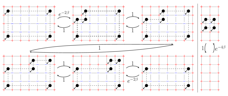
Figure 1: The spin configuration is represented by $+$ (red) and $-$ (blue) on the lattice. The black circles represent defects ($-1$ plaquette variables), which are associated with the vertex at the bottom left of the corresponding plaquette. Dashed lines separate regions of $+$ and $-$ spins. The labeled arrows indicate the associated transition rates. An isolated defect creates two defects at rate $e^{-2\beta}$, subsequently a pair of defects is emitted and moves along an edge of the rectangle according to a simple random walk, and is then annihilated upon colliding with another defect (possibly the defect that emitted the pair). Right: the only type of transition not included on the left is to add or remove four neighbouring defects.

Note that the “rectangular” configurations are entirely determined by the upper-left and lower-right vertices. Following the heuristic of Figure 1, these corner defects perform nearly-independent simple random walks as shown in Figure 2. A routine SRW calculation says that this rectangle will collapse to the unique ground state in a time that scales like $\Theta\left(e^{3.5\beta}\right)$. Since typical configurations have few defects, it is natural to guess that the relaxation time of these simple configurations will be very close to the relaxation time of the full process. This turns out to be correct, and will guide our proof.

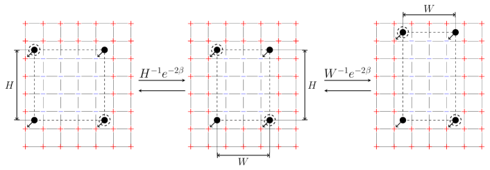
Figure 2: The defects at the corners of a box perform random walks at different rates: they move left-right at rate $H^{-1}e^{-2\beta}$ and up-down at rate $W^{-1}e^{-2\beta}$, where $H$ is the height of the box and $W$ is its width. These random walks are close to independent for $\beta$ large.

The canonical path method (see Section 5.1) can be used to extend this heuristic argument to configurations with many defects. If we restrict our attention to configurations whose defects form non-overlapping rectangles, the following canonical path construction would again give an $O(e^{3.5\beta})$ bound on the relaxation time:

1. Pick a rectangle uniformly at random.

2. Follow a minimal-length path that collapses this rectangle without ever adding more than 2 defects to the initial configuration, as given by the heuristic in Figures 1 and 2.

3. If any defects remain, go back to step (1).

In other words, if the rectangles don’t overlap, we can essentially treat them as evolving independently. Unfortunately, configurations with overlapping rectangles are possible. Allowing for overlaps, this simple path has very high congestion and so gives very poor bounds (see Figure LABEL:FigBadConfigNest). This problem occurs essentially becase the pairs of short-lived particles in Figure 2 can “interact” in this situation, and a similar problem is expected to occur in other plaquette models. In Section LABEL:SubsecPathLowDef we will show that it is possible to salvage our heuristic calculations by choosing rectangles according to a much more complicated rule. This rule is governed by a “soft” selection process that focuses on the most “prominent” rectangles. We use this to show that, on average, these interactions between short-lived defect pairs don’t contribute significantly to the congestion. We suspect that this basic approach can be used to analyze similar interacting-particle systems (in particular other plaquette models).

3 Main Results

We give bounds on the mixing and relaxation time of the square plaquette model on the critical scale:

Theorem 3.1 (Mixing and Relaxation Times for Plus Boundary Conditions).

The square plaquette process with all plus boundary conditions, on the critical scale, satisfies e^3.5 β ≲T_rel^+( L_c ) ≲β^6 e^3.5 β. Furthermore, e^3.5 β ≲T_mix^+( L_c ) ≲β^9 e^4 β.

Theorem 3.2 (Mixing and Relaxation Times for Periodic Boundary Conditions).

The square plaquette process with periodic boundary conditions, on the critical scale, satisfies e^4 β ≲T_rel^per( L_c ) ≲β^4 e^4 β. Furthermore, e^4 β ≲T_mix^per( L_c ) ≲β^9 e^4 β.

Remark 3.3.

With some extra technical effort in the canonical paths argument, the upper bound on the mixing time with plus boundary conditions can be improved (see [SPMcutoff] where it is shown that $T_{\rm mix}^{+}(L_{c})\lesssim\beta^{7}e^{3.75\beta}$). We conjecture that the lower bound given here is correct up to polynomial factors in $\beta$.

Remark 3.4.

We recall that the fundamental reason for the different scaling of the relaxation and mixing time with all plus and periodic boundary conditions is the structure of the ground states. With all plus boundary conditions there is a unique ground state (in which all sites have spin $+1$), and the low temperature dynamics are dominated by the time to reach the ground state. On the other hand, with periodic boundary conditions, the low temperature dynamics are dominated by an induced random walk on the $2^{2L-1}$ ground states. It turns out that this random walk behaves very similarly to the standard hypercube random walk.

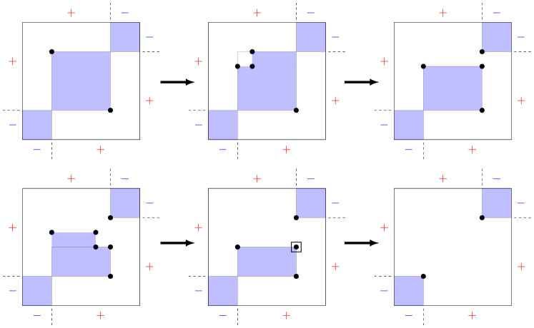
Figure 3: Two well separated ground states (top left and bottom right), with a typical path between them, as described in Remark 3.5. The shaded blue region indicates the $-$ spins, and the empty regions are $+$ spins.

Remark 3.5.

For certain special choices of boundary conditions, there exist a small number of ground states that are well separated, in the sense that it takes an extremely long time to switch between them. In the case of the boundary conditions given in Figure 3 we conjecture

$$e^{4.5\beta}\lesssim T_{\rm rel}^{\tau_{\rm bad}}(L_{c}).$$

The heuristic behind this bound is as follows. Typical paths between the two ground states are of the form described in the figure. Initially two new defects are created, at one of the existing defects, which occurs with rate $e^{-2\beta}$. Subsequently, with probability $1/L$, a pair of defects is not immediately re-absorbed, and travels a distance of order $L$. At some point during this excursion (top right frame of Fig. 2) the process may generates two new defects, with probability $\approx e^{-2\beta}L^{2}$. Subsequently, with probability $1/L$ again, these defects reach one of the isolated defects before being re-absorbed, leading to the stable configuration in the bottom middle Fig 2. Finally the defect marked with a square box makes a two dimensional random walk following the same mechanism as given in Figure 2. The projection of the position of this defect onto the diagonal (bottom left to top right) is a martingale, and so with probability $O(1/L)$ this defect will travel a distance $\Omega(L)$ before being re-absorbed in the previous ground state. Putting all these factors together gives the heuristic bound.

4 Preliminary Calculations and Notation

In this section, we make some simple observations about which configurations are possible and likely at stationarity. We first observe that only defect configurations satisfying certain parity constraints are possible, and these depend on the boundary conditions (Lemmas 4.1, and 4.2). These parity conditions immediately imply some rough bounds on the number of configurations with a given number of defects (Lemma 4.3), which in turn implies that the ground state has high probability under the stationary measure (Lemma 4.4).

In the case $\Lambda=[1:\ell_{1}]\times[1:\ell_{2}]$, we have $\mathcal{B}(\Lambda)=[0:\ell_{1}]\times[0:\ell_{2}]$. In this case we denote all the sites belonging to the $i^{\mathrm{th}}$ column of $\mathcal{B}(\Lambda)$ by $C_{i}=\{i\}\times[0:\ell_{2}]$, and the $j^{\mathrm{th}}$ row by $R_{j}=[0:\ell_{1}]\times\{j\}$. For $x,y\in\mathcal{B}(\Lambda)$ we write $y\ll x$ if $y_{1}<x_{1}$ and $y_{2}<x_{2}$.

Lemma 4.1 ($\tau$-b.c. parity constraints).

If $\Lambda=[1\!:\!\ell_{1}]\times[1\!:\!\ell_{2}]$ then for boundary condition $\tau\in\Omega$

$$p^{\tau}(\Omega_{\Lambda}^{\tau})=\{p\in\Omega_{\mathcal{B}(\Lambda)}\,:\,p\textrm{ satisfies \eqref{eq:par1} and \eqref{eq:par2} below}\}\,,$$

where the parity constraints are given by

$$\prod_{x\in C_{i}}p_{x} =\tau_{(i,0)}\tau_{(i+1,0)}\tau_{(i,\ell_{2}+1)}\tau_{(i+1,\ell_{2}+1)}\,,\quad\forall\,i\in[0:\ell_{1}]\quad\textrm{and,}$$ (4.1)

$$\prod_{x\in R_{j}}p_{x} =\tau_{(0,j)}\tau_{(0,j+1)}\tau_{(\ell_{1}+1,j)}\tau_{(\ell_{1}+1,j+1)}\,,\quad\forall\,j\in[0:\ell_{2}]\,.$$ (4.2)

Furthermore, $p^{\tau}:\Omega_{\Lambda}^{\tau}\to p^{\tau}(\Omega_{\Lambda}^{\tau})$ is bijective, and the inverse may be written as

$$(p^{\tau})^{-1}(p)_{x}=\sigma^{\tau}(p)_{x}:=\begin{cases}\tau_{(0,0)}\tau_{(x_{1},0)}\tau_{(0,x_{2})}\prod_{y\ll x}p_{y}&\textrm{if }x\in\Lambda,\\ \tau_{x}&\textrm{otherwise,}\end{cases}$$ (4.3)

for $p\in p^{\tau}(\Omega_{\Lambda}^{\tau})$.

Lemma 4.2 (Periodic b.c. parity constraints).

If $\Lambda=[0:\ell_{1}]\times[0:\ell_{2}]$ then for periodic boundary conditions

$$p^{\mathrm{per}}(\Omega_{\Lambda})=\{p\in\Omega_{\Lambda}\,:\,p\textrm{ satisfies \eqref{eq:parper} }\}\,,$$

where the parity constraints are given by

$$\prod_{x\in C_{i}}p_{x} =\prod_{x\in R_{j}}p_{x}=1\,,\quad\forall\,i\in[0:\ell_{1}-1]\quad\textrm{and}\quad\forall\,j\in[0:\ell_{2}-1]\,.$$ (4.4)

and for any fixed $\tau\in\{-1,1\}^{C_{0}\cup R_{0}}$, we have $p^{\mathrm{per}}:\{\sigma\in\Omega_{\Lambda}\,:\,\sigma_{C_{0}\cup R_{0}}\equiv\tau\}\to p^{\mathrm{per}}(\Omega_{\Lambda})$ is bijective.

Proof.

The proof relies on the following observation; for $\sigma\in\{-1,1\}^{\Lambda^{\prime}}$, for some $\Lambda^{\prime}$ finite, and $A,B\subset\Lambda^{\prime}$ we have

$$\prod_{x\in A}\sigma_{x}\prod_{y\in B}\sigma_{y}=\prod_{x\in A\triangle B}\sigma_{x}\,,$$ (4.5)

where $A\triangle B$ denotes the symmetric difference of $A$ and $B$. It follows that for $\sigma\in\Omega_{\Lambda}^{\tau}$ and $i\in[0:\ell_{1}]$

$$\prod_{x\in C_{i}}p_{x}^{\tau}(\sigma)=\prod_{x\in C_{i}}\prod_{y\in B_{x}}\sigma_{y}=\tau_{(i,0)}\tau_{(i+1,0)}\tau_{(i,\ell_{2}+1)}\tau_{(i+1,\ell_{2}+1)}\,,$$

and similarly for rows, i.e. $p^{\tau}(\Omega^{\tau}_{\Lambda})\subset\{p\in\Omega_{\mathcal{B}(\Lambda)}\,:\,p\textrm{ satisfies \eqref{eq:par1} and \eqref{eq:par2}}\}$.

To prove the opposite inclusion, fix $\zeta\in\{p\in\Omega_{\mathcal{B}(\Lambda)}\,:\,p\textrm{ satisfies \eqref{eq:par1} and \eqref{eq:par2}}\}$, then $\sigma^{\tau}(\zeta)\in\Omega_{\Lambda}^{\tau}$ by the definition given in (4.3). Furthermore, using (2.1) and (4.5),

$$p^{\tau}(\sigma^{\tau}(\zeta))_{x}=\prod_{y\in B_{x}}\sigma^{\tau}(\zeta)_{y}=\prod_{y\ll x}\zeta_{y}\prod_{z\ll x+e_{1}}\zeta_{z}\prod_{y^{\prime}\ll x+e_{2}}\zeta_{y^{\prime}}\prod_{z^{\prime}\ll x+e_{1}+e_{2}}\zeta_{z^{\prime}}=\zeta_{x}$$

This completes the proof of Lemma 4.1, since $|\Omega_{\Lambda}^{\tau}|=|\{p\in\Omega_{\mathcal{B}(\Lambda)}\,:\,p\textrm{ satisfies \eqref{eq:par1} and \eqref{eq:par2}}\}|=2^{|\Lambda|}$. The proof of Lemma 4.2 follows the same arguments. ∎

These parity considerations imply the following bounds on the number of configurations with a given number of defects:

Lemma 4.3.

Fix $k\in\mathbb{N}$. If $\Lambda=[1:L]^{2}$, then with all plus boundary conditions

$$|\{\sigma\in\Omega_{\Lambda}^{+}\,:\,|p^{+}(\sigma)|=2k\}|\;\leqslant\;\min\{(ek)^{2k}L^{2k},L^{3k}\}\,.$$ (4.6)

If $\Lambda=[0:L]^{2}$, then with periodic boundary conditions

$$|\{\sigma\in\Omega_{\Lambda}\,:\,|p^{\mathrm{per}}(\sigma)|=2k\}|\;\leqslant\;2^{2L+1}\min\{(ek)^{2k}L^{2k},L^{3k}\}\,.$$ (4.7)

Proof.

We begin with the $+$ boundary conditions. By Lemma 4.1 we have, for each $k\in\mathbb{N}$,

$$|\{\sigma\in\Omega_{\Lambda}^{+}\,:\,|p^{+}(\sigma)|=2k\}|=|\{p\in p^{+}(\Omega_{\Lambda}^{+})\,:\,|p|=2k\}|$$

and $|\{p\in p^{+}(\Omega_{\Lambda}^{+})\,:\,|p|=2k\}|$ is exactly the number of configurations in $\{0,1\}^{\Lambda}$, where we identify defects with $1$’s, which have even row and column sums and the total number of defects is $2k$. Since any row which contains at least one defect must also contain at least two, the total number of rows which have at least one defect is clearly bounded above by $k$ (similarly for columns). It follows that the number of configurations which satisfy the row and column parity constraint is at most the number of ways of firstly choosing $k$ rows and $k$ columns (with replacement), and then arranging the $2k$ defects anywhere on the sub-lattice defined by these rows and columns. The number of ways of arranging the former is $L^{2k}$, and the number of ways of arranging the latter is clearly bounded above by $\binom{k^{2}}{2k}$. Using $\binom{n}{k}<(e\,n)^{k}/k^{k}$ and taking the product gives the first upper bound. The second upper bound follows by using only the row parity, which implies that the defects may be grouped into $k$ disjoint pairs, such that defects belonging to the same pair occupy the same row. There are then at most $L^{3}$ ways to arrange each pair on $\Lambda$ and the upper bound $L^{3k}$ follows immediately.

We next consider periodic boundary conditions. By the above argument, for every choice of $\tau\in\{-1,1\}^{C_{0}\cup R_{0}}$ we have —{σ∈Ω_Λ :  —p^per(σ)— = 2k,   σ—_C_0 ∪R_0 = τ}—  ⩽ min{(e k)^2k L^2k,L^3k}. Applying the bijection in Lemma 4.2 and noting that $|\{-1,1\}^{C_{0}\cup R_{0}}|=2^{2L+1}$ completes the proof. ∎

For a given boundary condition $\tau$, define the collection of ground states by:

$$\mathcal{G}=\mathcal{G}^{\tau}=\{\sigma\in\Omega_{\Lambda}^{\tau}\,:\,H_{\Lambda}^{\tau}(\sigma)=\min_{\eta\in\Omega_{\Lambda}^{\tau}}H_{\Lambda}^{\tau}(\eta)\}.$$ (4.8)

Lemma 4.4 (Domination of Ground States).

Let $\tau\in\{+,\rm{per}\}$ and $L=L_{c}$, then

$$\pi(\mathcal{G})\;\geqslant\;1-O(e^{-2\beta})\,.$$ (4.9)

Proof.

By Lemmas 4.1 and 4.2, we note that all possible configurations have an even number of defects, and also that no configurations can have exactly 2 defects. When $\tau=+$, there is a unique ground state $+\equiv(+1,\ldots,+1)$. In this situation, Lemma 4.3 gives

$$1-\pi(+) =\sum_{k\;\geqslant\;2}\pi(+)|\{\sigma\in\Omega_{\Lambda}^{+}\,:\,|p^{+}(\sigma)|=2k\}|e^{-2k\,\beta}\lesssim\pi(+)e^{-2\beta}\,.$$

Thus $\pi(+)=1-O(e^{-2\beta})$, completing the proof of the lemma for $\tau=+$. For the case of periodic boundary conditions, observe that there are exactly $2^{2L+1}$ ground states, so $\pi(\mathcal{G})=2^{2L+1}\pi(+)$ and the same argument holds. ∎

5 Construction and Analysis of Canonical Paths

Our arguments for the upper bounds in Theorems 3.1 and 3.2 will be based on the method of “canonical paths.” The idea in this method is to construct a family of (possibly random) paths between any pairs of configurations $\sigma,\eta$, such that the paths do not use any one edge too much. In this section, we construct the canonical paths that will be used for those proofs, and also give some initial analysis of their properties. As a guide to the remainder of this section:

• In Section 5.1, we state generic bounds on relaxation and mixing times of a Markov chain in terms of canonical paths. These are small variants of well-known results, but may be useful in the study of other Markov chains.

• In Section LABEL:SubsecPrelPathNot, we give preliminary notation related to canonical paths.

• In Section LABEL:SubsecPathLowDef, we construct and analyze the main “building block” of our canonical path construction. This building block determines the entire path for any initial configuration $\sigma$ with $O(\beta L)$ defects.

• In Section LABEL:SubsecPathHighDef, we construct a “building block” that may be used when $\sigma$ has many more than $L$ defects. We also combine our two building blocks to construct the main canonical path used throughout this paper.

• In Section LABEL:SecPathAnalysisLemmas, we give simple bounds on various quantities related to combining the building blocks into a longer canonical path.

• In Section LABEL:SecFinalBoundCanonical, we combine the results in this section to obtain final bounds on the properties of the canonical paths we have defined.

5.1 Canonical Path Bounds

In this section we describe the use of canonical path arguments to bound the spectral gap and spectral profile of a Markov process on finite state space. We first set some standard notation for this subsection only. For a general Markov chain with transition rate matrix $K$ on state space $\Omega$, denote by $\mathbf{E}=\{(\eta,\sigma)\in\Omega^{2}\,:\,K(\eta,\sigma)>0\}$ the collection of transitions allowed by $K$. We recall the notion of paths in such a Markov chain:

Definition 5.1 (Path).

A sequence $\gamma=(\eta^{(0)},\eta^{(1)},\ldots,\eta^{(m)})\in\Omega$ is called a path from $\eta^{(0)}$ to $\eta^{(m)}$ if $(\eta^{(i-1)},\eta^{(i)})\in\mathbf{E}$ for all $1\;\leqslant\;i\;\leqslant\;m$. We say that this path has length $|\gamma|\equiv m$. For $1\;\leqslant\;i\;\leqslant\;m$, we call the pair $(\eta^{(i-1)},\eta^{(i)})$ the $i$’th edge of $\gamma$. For $\eta,\sigma\in\Omega$, we denote by $\Gamma_{\eta,\sigma}$ the collection of all paths from $\eta$ to $\sigma$. Similarly we let $\Gamma_{\eta}=\cup_{\sigma}\Gamma_{\eta,\sigma}$ be the collection of all paths starting at $\eta$ and $\Gamma=\cup_{\eta,\sigma\in\Omega_{\Lambda}}\Gamma_{\eta,\sigma}$ be the collection of all paths.

For a path $\gamma=(\eta^{(0)},\ldots,\eta^{(m)})$, we denote by $\gamma^{(\mathrm{init})}=\eta^{(0)}$ and $\gamma^{(\mathrm{fin})}=\eta^{(m)}$ the initial and final elements of $\gamma$. If $\gamma_{1}$, $\gamma_{2}$ are two paths with $\gamma_{1}^{(\mathrm{fin})}=\gamma_{2}^{(\mathrm{init})}$, we denote by $\gamma_{1}\bullet\gamma_{2}$ the concatenation of $\gamma_{1}$ and $\gamma_{2}$ with the repeated element $\gamma_{1}^{(fin)},\gamma_{2}^{(init)}$ removed. With some abuse of notation, we define $\emptyset\bullet\gamma=\gamma\bullet\emptyset=\gamma$ for any path $\gamma$.

When applying the results in this Section, we will always use the process given by (2.8).

For the remainder of this section, assume that $K$ has a unique reversible measure $\mu$ and let $\mu_{\ast}=\min_{\eta\in\Omega}\mu(\eta)$. For $S\subset\Omega$, define $c_{0}(S)$ to be the non-constant functions on $\Omega$ with support contained in $S$. For $S\subset\Omega$, also define λ(S) = inf_f ∈c_0(S) DK(f)Varμ(f), where $\mathcal{D}_{K}$ is the Dirichlet form associated with $K$, D_K = -μ(f Kf)= 12∑_η,σ∈Ωμ(η)K(η,σ)(f(η)-f(σ))^2 .

Lemma 5.2 (Multicommodity Flows for Bounding the Spectral Profile).

Let $S\subsetneq\Omega$. For $\eta\in S$, let $F_{\eta}$ be a probability measure on paths $\gamma=(\gamma^{0},\ldots,\gamma^{m})$ in $\Omega$ that have starting point $\gamma^{0}=\eta$ and final point $\gamma^{m}\in S^{c}$. Then

λ(S)  ⩾ A^-1, where A ≡2  max_e ∈E ∑_η∈Ω ∑_γ∋e F_η(γ)   — γ—   μ(η)μ(e-) K(e-,e+) is the cost of the flow $\{F_{\eta}\}_{\eta\in S}$.

Remark 5.3.

We will use this with $S=\Omega_{\Lambda}\backslash\{+\}$ when bounding the spectral gap of the SPM with + boundary conditions. The more general bound is useful for bounding the spectral profile, which we will need to obtain a more refined mixing time bound.

Proof.

Fix $f\in c_{0}(S)$ with $\mathbb{E}_{\mu}[f]=0$. By the Cauchy-Schwarz inequality and the fact that $f(y)=0$ for all $y\in S^{c}$, Var_μ(f) &= ∑_η∈Ω μ(η) f(η)^2 = ∑_η∈Ωμ(η) ∑_γ F_η(γ) ( ∑_i=1^—γ— (f(γ^i-1) - f(γ^i)))^2
 ⩽ ∑_η∈Ω ∑_γ μ(η)F_η(γ)   — γ—   ∑_i=1^—γ— (f(γ^i-1) - f(γ^i))^2
= ∑_η∈Ω ∑_γμ(η) F_η(γ)   — γ—   ∑_i=1^—γ— μ(γi-1) K(γi-1, γi)μ(γi-1) K(γi-1, γi) (f(γ^i-1) - f(γ^i))^2. Comparing this to the formula for the Dirichlet form, this gives Varμ(f)DK(f)  ⩽ 2  max_e ∈E ∑_η∈Ω ∑_γ∋e F_η(γ)   — γ—   μ(η)μ(e-) K(e-,e+), completing the proof of the lemma.

∎

This bound is all that we will require to bound the spectral gap of the SPM model with + boundary conditions. In order to bound the mixing time of both chains, as well as the spectral gap of the SPM with periodic boundary conditions, we will use the spectral profile method introduced in [Goel2006]. We quickly recall the main results of that paper:

Definition 5.4 (Spectral Profile Bounds.).

For $r>0$, define Λ(r) = inf_μ_∗  ⩽ μ(S)  ⩽ r λ(S). Theorem 1.1 of [Goel2006] states that the mixing time $T_{\rm mix}$ of $K$ satisfies T_mix ⩽ ∫_4   μ_∗^16 2x   Λ(x) dx.

In our application, the spectral profile $\Lambda(r)$ is defined as an infimum over a very large collection of subsets $S\subset\Omega_{\Lambda}^{\tau}$; we will find it easier to work with a much-reduced collection of subsets. For fixed $r>0$, let k(r) = min{ k   :   π(+)   e^-βk  ⩽ r }. For fixed $k\in\mathbb{N}$, let S