Uncertainty in the Variational Information Bottleneck

Abstract

We present a simple case study, demonstrating that Variational Information Bottleneck (VIB) can improve a network’s classification calibration as well as its ability to detect out-of-distribution data. Without explicitly being designed to do so, VIB gives two natural metrics for handling and quantifying uncertainty.

1 Introduction

It is important to track and quantify uncertainty. Prediction uncertainty is a consequence of one or more non-exclusive sources including (Gal, 2016), but not limited to: aleatoric uncertainty, (e.g., noisy data or measurement imprecision) epistemic uncertainty, (e.g., unknown model parameters, unknown model structure) and out-of-distribution samples (e.g., train/eval datasets do not share the same stochastic generator).

Ideally a model should have some sense of whether it has sufficient evidence to render a prediction. Adversarial examples (Szegedy et al., 2013) demonstrate a broad failure of existing neural networks to be sensitive to out-of-distribution shifts, but distributional shifts don’t require an adversary–any deployment of a model in a real-world system is likely to encounter surprising out-of-distribution data.

Most classifiers report probabilities. Models which do this well are said to be calibrated – the observed occurrence frequency matches the predicted frequency (Brier, 1950). If the model assigns a 20% probability to an event, that event should occur 20% of the time. Current deep networks tend to be poorly calibrated (Guo et al., 2017), making highly confident predictions even when they are wrong.

Many recent papers (Guo et al., 2017; Lakshminarayanan et al., 2016; Hendrycks & Gimpel, 2016; Liang et al., 2017; Lee et al., 2017; DeVries & Taylor, 2018) have proposed techniques for improving the quantification of uncertainty in neural networks. The simplest such modification, temperature scaling (Guo et al., 2017; Hendrycks & Gimpel, 2016; Liang et al., 2017), changes the temperature of the softmax classifier after training for use during prediction. It empirically does well at improving the calibration and out-of-distribution detection for otherwise unmodified networks. Other approaches require larger interventions or modifications, e.g. training on out-of-distribution data directly, generated either in an adversarial fashion (Liang et al., 2017; Lee et al., 2017) or chosen by the practitioner (DeVries & Taylor, 2018).

Instead of specifically trying to invent a new technique for improved calibration, this work empirically demonstrates that the previously described variational information bottleneck (VIB) (Alemi et al., 2017) gives calibrated predictions and does a decent job at out-of-distribution detection without sacrificing accuracy.

2 Variational Information Bottleneck

Variational Information Bottleneck (VIB) (Alemi et al., 2017) learns a variational bound of the Information Bottleneck (IB) (Tishby & Zaslavsky, 2015). VIB is to supervised learning what $\beta$-VAE (Higgins et al., 2017) is to unsupervised learning; both are justified by information theoretic arguments (Alemi et al., 2018).

IB regards supervised learning as a representation learning problem, seeking a stochastic map from input data $X$ to some latent representation $Z$ that can still be used to predict the labels $Y$, under a constraint on its total complexity.

Writing mutual information between random variables $Z,Y$ as $I(Z;Y)$, the information bottleneck procedure is:

$$\max I(Z;Y)\text{ subject to }I(Z;X)\leq R$$ (1)

where $R$ is a constant bottleneck. Rewritten as an unconstrained Lagrangian optimization, the procedure is:

$$\max I(Z;Y)-\beta I(Z;X)$$ (2)

where $\beta$ controls the size of the bottleneck.

IB is intractable in general. However, there exists a simple tractable variational bound (Alemi et al., 2017):

$$\max_{\theta,\phi,\psi}\mathbb{E}_{p(x,y)e_{\theta}(z|x)}\left[\log q_{\psi}(y|z)-\beta\log\frac{e_{\theta}(z|x)}{m_{\phi}(z)}\right]$$ (3)

The $q$ term measures classification log likelihood and the $\frac{e}{m}$ term represents rate, penalizing lengthy encodings $e$ relative to some code space, $m$. More precisely:

• $e_{\theta}(z|x)$ is a learned stochastic encoder that transforms the input $X$ to some encoding $Z$;

• $q_{\psi}(y|z)$ is a variational classifier, or decoder that predicts the labels $Y$ from the codes;

• $m_{\phi}(z)$ is a variational marginal that assigns a density in the code space; and

• $p(x,y)$ is the empirical data distribution.

VIB incorporates uncertainty in two ways. VIB is doubly stochastic in the sense that both the underlying feature representation ($Z$) and the labels ($Y$) are regarded as random variables. Conversely, DNNs only regard the labels as being random variables. By explicitly modeling the representation distribution, VIB has the ability to model both mean and variance in the label predictions. Recall that for most DNNs, the output layer corresponds to a distribution in which variance is a function of mean (e.g., a binary classifier predicting $p$ for a class occurrence must also predict the variance $p(1-p)$). The stochasticity in the representation induces an effective ensemble of decoder predictions. Ensembles of whole neural networks have been shown to be well calibrated (Lakshminarayanan et al., 2016).

The second source of uncertainty is provided by the per-instance rates. Recall that the rate is the KL divergence between the conditional distribution over codes given the input and the code space defined by the learned marginal $m_{\phi}(z)$; i.e. $\operatorname{KL}[e_{\theta}(z|x)||m_{\phi}(z)]$. Here, the marginal effectively learns a density model for the data, albeit in the lower-dimensional, lower-information code-space rather than the original input space. Density estimation, whether explicit (DeVries & Taylor, 2018) or implicit (Kliger & Fleishman, 2018), has been shown to be useful for out-of-distribution detection.

A stochastic representation requires computing an additional expectation at both training and test time. We find that approximating the expectation with a Monte Carlo average with a few dozen samples produces surprisingly low variance predictions. In practice, the bulk of the model complexity is in the encoding network (typically a deep convolutional network), which need only be run once to obtain the parameters for the encoding distribution. We find that very low dimensional distributions (e.g. 3D fully covariant Gaussians) and simple variational decoders (a mixture of softmaxes (Yang et al., 2018)) work well. For these, sampling and evaluating the log likelihoods is dwarfed by the initial encoder, and so VIB has little effect on computation time.

3 Experiments

Below we demonstrate results of training a VIB classifier on FashionMNIST (Xiao et al., 2017). We compare the network’s ability to both quantify the uncertainty in its own predictions on the test set, as well as identify when shown out-of-distribution data.

For our encoder we used a 7-2-WRN (Zagoruyko & Komodakis, 2016) initialized with the delta-orthogonal initializer (Xiao et al., 2018) and bipolar-relu non-linearities (Eidnes & Nøkland, 2017) topped with a 3-dimensional fully covariant Gaussian encoding distribution. Given the strong spatial inhomogeneities of the data, we concatenated a $28\times 28\times 5$ set of learned parameters to the original image before feeding it through the network. The variational marginal is a mixture of 200 3-dimensional fully covariant Gaussians. The decoder is a Categorical mixture of five Categorical distributions with affine logits. For the baseline deterministic network, the 7-2-WRN feeds directly into a logistic classifier . The networks were trained with a 0.1 dev-decay (Wilson et al., 2017) with Adam (Kingma & Ba, 2015), with initial learning rate of 0.001. All other hyperparameters are set to the TensorFlow defaults. We emphasize that we used no form of regularization aside from VIB.

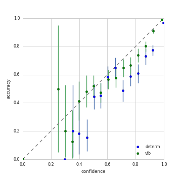
Figure 1: Reliability diagram for the trained networks. This shows how well-calibrated the networks are. The predictions were split into 20 equally-sized bins. The accuracy was measured in each bin. Shown is the accuracy as well as the 90% confidence interval for the accuracies. A perfectly calibrated model would fall on the diagonal.

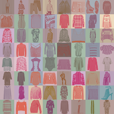
(a) Lowest classification confidence examples.

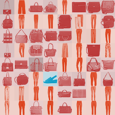
(b) Highest classification confidence examples.

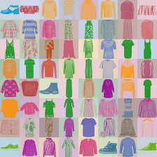
(c) Highest confidence misclassification examples.

(d) Random selection.

(e) Color Legend for the FashionMNIST classes.

Figure 2: Extreme examples from the test set. Images from the test set are shown colored according to a weighted combination of the class colors in Figure 2(e). The background lightness shows $R$, and the background hue is the correct class.

Method	Accuracy	Threshold	FPR @95% TPR $\downarrow$	AUROC $\uparrow$	AUPR In $\uparrow$	AUPR Out $\uparrow$
Baseline	92.9	$H$	45.3	91.3	99.3	03.8
Baseline T			83.0	74.7	97.6	04.3
VIB	92.8	$H$	44.8	91.2	99.2	03.8
		$R$	63.1	84.7	98.6	03.9

Table 1: Results on error detection. Here we use the threshold signal to try to distinguish correct and incorrect predictions. Arrows denote whether higher or lower scores are better. Bold indicates the best score in that column. Bold italics indicate the closest VIB score if a baseline score was better. Baseline T is with temperature scaling. VIB mostly matches performance. For VIB, $H$ is better at error detection than $R$, while the opposite is true with OoD detection.

OoD	Method	Threshold	FPR @ 95% TPR $\downarrow$	AUROC $\uparrow$	AUPR In $\uparrow$	AUPR Out $\uparrow$
U(0,1)	Baseline	$H$	79.5	87.3	91.2	32.9
	Baseline T		00.6	99.2	99.5	30.7
	VIB	$H$	43.8	90.8	91.0	31.8
		$R$	09.6	97.6	98.0	30.9
MNIST	Baseline	$H$	78.4	73.2	75.4	36.1
	Baseline T		41.9	88.9	90.8	31.8
	VIB	$H$	63.3	83.2	83.2	33.4
		$R$	27.3	92.7	92.0	31.4
HFlip	Baseline	$H$	86.7	66.0	64.4	39.8
	Baseline T		77.1	67.8	64.7	39.3
	VIB	$H$	81.1	65.7	59.8	42.3
		$R$	73.0	68.7	64.4	39.3
VFlip	Baseline	$H$	64.5	85.6	87.8	32.8
	Baseline T		38.5	92.1	94.1	31.5
	VIB	$H$	45.0	86.4	83.4	32.6
		$R$	34.4	89.7	87.0	32.0

Table 2: Results for out-of-distribution detection (OoD). Arrows denote whether higher or lower scores are better. Bold indicates the best score in that column for a particular out-of-distribution dataset. Bold italics indicate VIB scores that are better than the Baseline row.

Metrics.

We can compare the ability of various signals to distinguish misclassified examples beyond the reported probability ($p(y|x)$). For instance, we can look at the entropy of the classifier $H(y|x)=-\sum_{i}p(y_{i}|x)\log p(y_{i}|x)$ ($H$ in the tables); or in the case of VIB networks, the rate ($R$ in the tables) and $p(y,z|x)=\int dx\,p(x)e_{\theta}(z|x)q_{\psi}(y|z)\approx m_{\phi}(z)q_{\psi}(y|z)$, the conditional joint likelihood. See Appendix A for results and discussion of all four metrics. Here we focus on $H$ and $R$.

Since these are not necessarily calibrated measures themselves, we compute threshold independent metrics (AUROC, AUPR) as done in Hendrycks & Gimpel (2016); Liang et al. (2017) (See references for detailed definitions of metrics). In Tables 1 and 2, FPR is the false positive rate, TPR is the true positive rate, AUROC is the area under the ROC curve, and AUPR is the area under the precision-recall curve. AUPR is sensitive to which class is denoted as positive, so both versions are reported. AUPR In sets the in-distribution examples as positive. AUPR Out sets the out-of-distribution examples as positive.

Discussion.

In Figure 1 we demonstrate that the VIB network is better-calibrated than the baseline deterministic classifier. The deterministic classifier is overconfident.

We report error detection results in Table 1. Note that the deterministic baseline and VIB perform equivalently well across the board. Baseline T in the tables is the baseline model tested at a temperature of 100. $H$ seems to offer better error detection than $R$ for the VIB network.

Next we measure the ability to detect out-of-distribution data. We take the same networks, trained on FashionMNIST, and then evaluate them on the combination of the original FashionMNIST test set, as well as another test set. We evaluate the ability of each metric to distinguish between the two. We compare against randomly generated images (U(0,1), for uniform noise) and MNIST digits to get a measure of gross distribution shift. We also test on horizontally and vertically flipped FashionMNIST images for more subtle distributional shift. We believe these offer an interesting test since the FashionMNIST data has a strong orientation – the clothes have clear tops versus bottoms, and for the shoes, care was taken to try to have all the shoes aligned to the left. Since these modified image distributions are just mirrored versions of the original, all of the mirror invariant statistics of the images are unchanged by this operation, suggesting this is a more difficult situation to resolve than the first two test sets.

From Table 2 we can draw a few early conclusions. Temperature scaling remains a powerful post-hoc method for improving the calibration and out-of-distribution detection of networks. It additionally improved the performance of our VIB networks (not shown here), but here we emphasize that VIB networks offer an improvement over the baseline without post-hoc modification. Without relying on temperature scaling, a VIB network can use $R$ for stronger out-of-distribution detection.

To visually demonstrate the different measures of uncertainty in the VIB network, in Figure 2 we show some of the extreme inputs. Interestingly, the network has instances where the rate is low (signifying that it thinks the example is valid clothing) but that have high predictive entropy (signifying that the network doesn’t know how to classify them) as well as the converse–things that look outside the training distribution, but the network is certain they are of a particular class. E.g., in Figure 2(a) there are some examples with both low rate and low classification confidence. These examples are within the data distribution as far as the network is concerned, but it is uncertain about their class, often splitting its prediction equally across two options. In Figure 2(b) we see the opposite, with some examples like the first having very high classification confidence (the network is certain that is a handbag), but with high rate (it is unlike most other handbags, given its unusually long handle). This sort of distinction is not possible in ordinary networks. Figure 2(c) shows the most confidently misclassified examples from the test set. Arguably, a majority of these instances are mislabelings in the test set itself. Figure 2(d) shows a representative sample of images from the test set for comparison. Figures 5, 6 and 7 in Appendix A show the complete test set, as well as its mirrored versions.

4 Conclusion

While more experimentation is needed, initial investigations suggest that VIB produces well-calibrated networks, while also giving quantitative measures for detecting out-of-distribution samples. Coupled with VIB’s other demonstrated abilities to improve generalization, robustness to adversarial examples, preventing memorization of random labels, and becoming robust to nuisance variables (Alemi et al., 2017; Achille & Soatto, 2017), we believe it deserves more investigation experimentally and theoretically.

Appendix A Appendix

Here we show more detailed images and tables for our results.

Figure 3 shows how the rate responds as we flip the images vertically and horizontally on a per-class basis. It demonstrates the model has learned useful semantics regarding the orientation of the clothes categories.

Figure 4 shows a visualization of the latent space of a VIB model with the same architecture as the model described in the paper, but with a 2D latent space rather than 3D. In general we can train accurate classifiers with very low dimensional representations. Note that the images with red arrows, which are the 10 highest rate ($R$) examples in the test set, occur either near classification boundaries, or far away from the high density regions. However, they are not necessarily incorrectly classified. For example, all three images in the lower right are images of pants that are correctly classified. The two images with red arrows are images that contain two pairs of pants, which is unusual in the dataset. Similarly, the highest rate images are not all out-of-distribution as defined by vertical flip. In fact, only 5 of the top 10 highest rate images are vertically flipped in this model with this set of samples. Of the remaining 5, two are the previously mentioned pants, two are “unusual” coats according to the model, and the final one has a true label of “sandal”, but is mislabeled by the model as “sneaker”.

Figures 5, 6 and 7 show the complete FashionMNIST test sets, with $p(y|x)$, $H(y|x)$, and $R$ visualized in orthogonal manners. Comparing the Figures against one another, you can see interesting relationships between the classes and the mirror transformations. For instance there is some tendency for vertically flipped pants to classify as dresses and vice versa. Under horizontal flips most classes are well-behaved, while all of the footwear classes show marked increase in the rates.

Tables 3 and 4 give a more detailed view of the different models and datasets used. In these tables, we present all four different metrics: $p(y|x)$, the standard signal used in out-of-distribution detection; $H(y|x)$, which generally outperforms $p(y|x)$ and can be used anywhere $p(y|x)$ can be used; $p(y,z|x)$, which does well at improving false-positive-oriented metrics, like FPR @95% TPR and AUPR Out, but which requires a density model of the latent space, such as the one learned by VIB; and $R$, the rate, which seems to perform well at out-of-distribution detection, and which also requires a density model of $z$.

Table 3 gives more data comparing the deterministic baselines with the VIB model for error detection. Note that the deterministic baseline and VIB perform equivalently well across the board. This is unsurprising, since if the models had a clear signal to discriminate between true and false positives in the in-sample data, the optimization procedure should be able to find that signal and use it to directly improve the objective function.

From Table 4 we can draw a few early conclusions. VIB generally dominates the deterministic baseline at T=1. $R$ is strong at out-of-distribution detection. $p(y,z|x)$ is strong at gross error detection (U(0,1) and MNIST FPR @95% TPR), as well as subtle error detection (HFlip and VFlip AUPR Out). $p(y|x)$ and $H(y|x)$ without temperature scaling only dominate at error detection for the gross errors (U(0,1) and MNIST AUPR Out). However, $H(y|x)$ and $p(y,z|x)$ (not shown) are very responsive to temperature scaling, giving substantial improvements across the board for both the deterministic model and VIB (not shown).

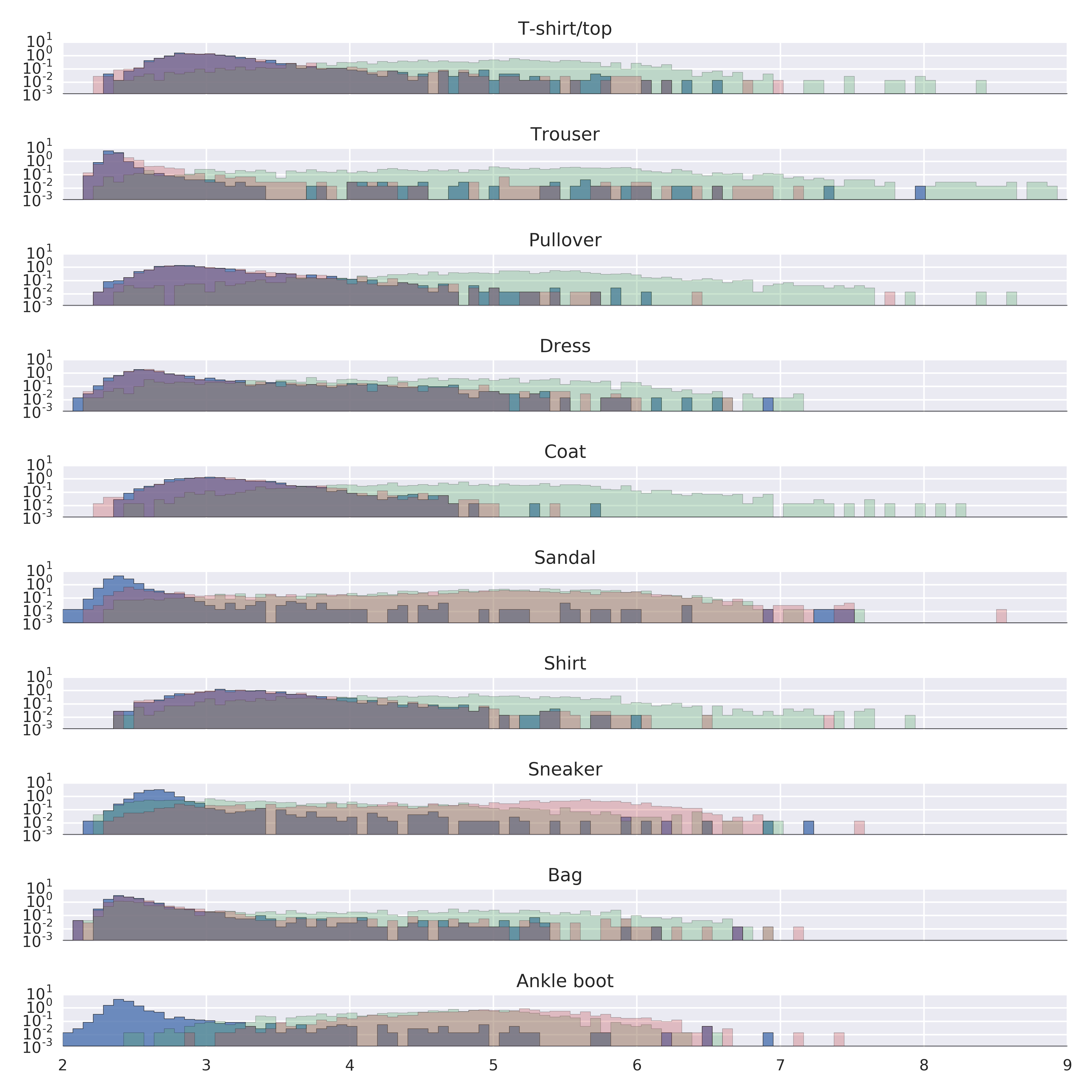
Figure 3: Demonstration of the change in rates when we perturb the images. The original test set histogram is in blue, the vertically flipped images are in green, and the horizontally flipped images are in red. Notice that this is a log-histogram, and there is very little overlap between the original images and the vertically flipped ones in any class. For most classes there is a great deal of overlap between the original images and the horizontally flipped ones, except for Sandal, Sneaker, and Ankle Boot, which have a strong left-right asymmetry.

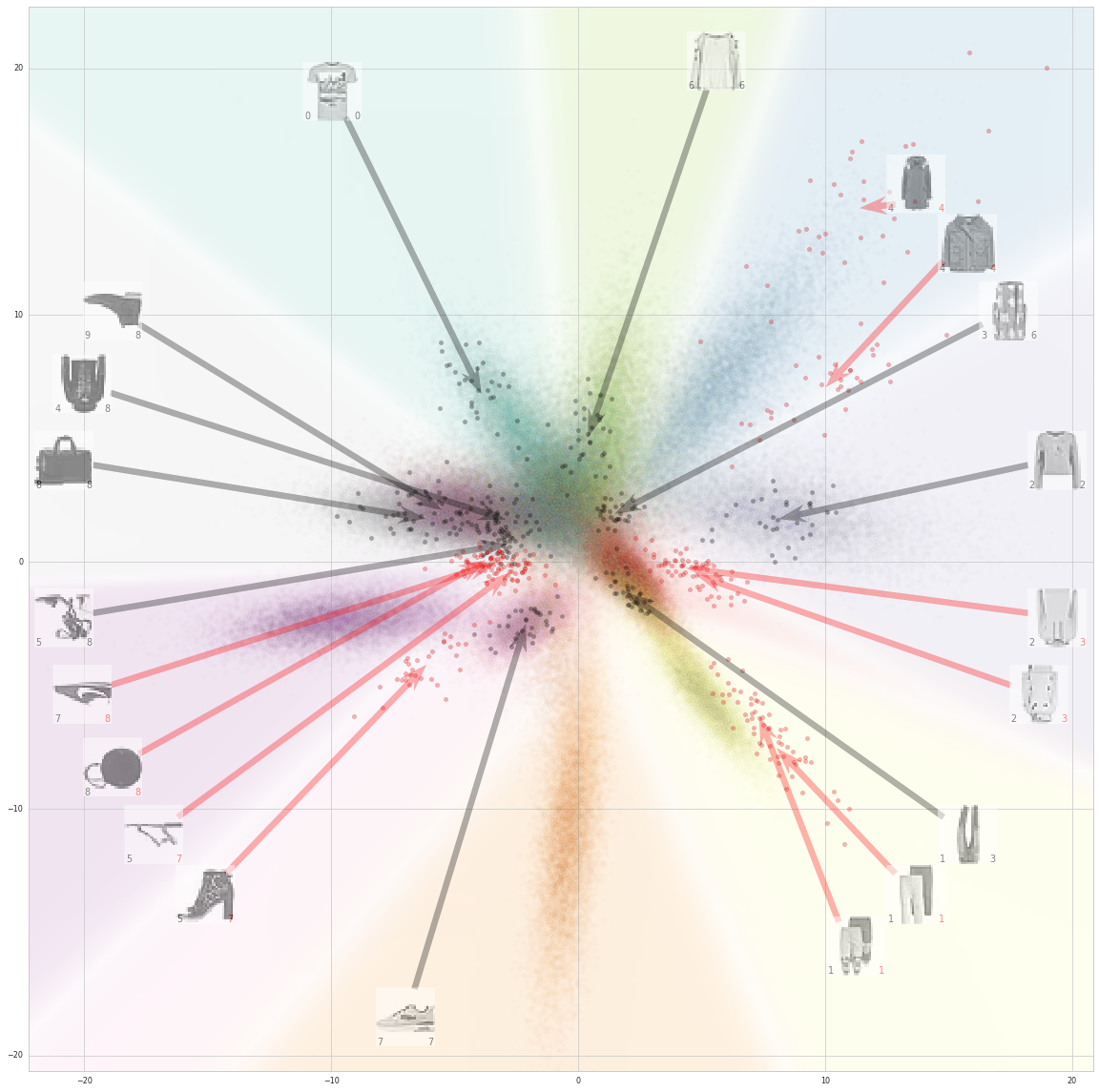
Figure 4: Visualization of a VIB model’s 2D latent space. The background color corresponds to the mixture of classes predicted by the classifier for that location in $z$ space. Transparency increases as the confidence of the maximum class decreases, so the light white lines in the image correspond to a high $H(Y|Z)$. More saturated regions correspond to higher marginal densities, $m(z)$. The colored points are the $z$ locations for 20,000 test set images – 10,000 normal images, and 10,000 vertically-flipped images. The color of each point indicates its true label, and should match the color of the background. Additionally, 10 clouds of dark grey points are randomly selected images from the test set, 1 for each class. Each cloud corresponds to the 32 samples from the encoder taken for each input. The clouds show the variance in the encoding distribution. Images with dark grey arrows point to the mean of the corresponding cloud of 32 samples. Finally, 10 clouds of dark red points are the 10 images from the test set with the highest mean rate, $R$. Similarly, the images with dark red arrows point to the mean of the corresponding cloud of 32 encoder samples.

Figure 5: Fashion MNIST. The complete test set. Foreground color is the weighted mixture of the predicted class colors. Background darkness is the per-instance rate. The images are ordered first by the true class into blocks, and then in each block by maximum $p(y|x)$.

Figure 6: The same visualization as in Figure 5 but for the vertically flipped FashionMNIST test set.

Figure 7: The same visualization as in Figure 5 but for the horizontally flipped FashionMNIST test set.

Method	Accuracy	Threshold	FPR @95% TPR $\downarrow$	AUROC $\uparrow$	AUPR In $\uparrow$	AUPR Out $\uparrow$
Baseline T=1	92.9	$p(y|x)$	44.8	91.9	87.8	03.8
		$H(y|x)$	45.3	91.3	99.3	03.8
Baseline T=100		$p(y|x)$	65.2	87.1	98.9	03.9
		$H(y|x)$	83.0	74.7	97.6	04.3
VIB T=1	92.8	$p(y|x)$	45.6	91.3	99.2	03.8
		$H(y|x)$	44.8	91.2	99.2	03.8
		$p(y,z|x)$	69.3	83.4	98.3	04.0
		$R$	63.1	84.7	98.6	03.9

Table 3: Extended results on error detection. Arrows denote whether higher or lower scores are better. Bold indicates the best score in that column. Bold italics indicate the closest VIB score if a baseline score was higher.

OoD	Method	Threshold	FPR @ 95% TPR $\downarrow$	AUROC $\uparrow$	AUPR In $\uparrow$	AUPR Out $\uparrow$
U(0,1)	Determ. T=1	$p(y|x)$	81.7	86.8	80.2	33.0
		$H(y|x)$	79.5	87.3	91.2	32.9
	Determ. T=100	$p(y|x)$	10.5	97.7	98.4	31.0
		$H(y|x)$	00.6	99.2	99.5	30.7
	VIB T=1	$p(y|x)$	54.7	90.0	90.6	32.0
		$H(y|x)$	43.8	90.8	91.0	31.8
		$p(y,z|x)$	14.4	95.9	96.8	31.0
		$R$	09.6	97.6	98.0	30.9
MNIST	Determ. T=1	$p(y|x)$	82.6	72.9	64.0	36.2
		$H(y|x)$	78.4	73.2	75.4	36.1
	Determ. T=100	$p(y|x)$	51.9	85.5	86.3	32.7
		$H(y|x)$	41.9	88.9	90.8	31.8
	VIB T=1	$p(y|x)$	69.6	82.4	83.0	33.5
		$H(y|x)$	63.3	83.2	83.2	33.4
		$p(y,z|x)$	39.7	86.1	82.6	32.8
		$R$	27.3	92.7	92.0	31.4
HFlip	Determ. T=1	$p(y|x)$	88.0	65.7	56.1	38.7
		$H(y|x)$	86.7	66.0	64.4	39.8
	Determ. T=100	$p(y|x)$	79.2	68.9	65.7	38.9
		$H(y|x)$	77.1	67.8	64.7	39.3
	VIB T=1	$p(y|x)$	83.7	65.1	59.5	42.5
		$H(y|x)$	81.1	65.7	59.8	42.3
		$p(y,z|x)$	79.0	62.5	57.3	43.7
		$R$	73.0	68.7	64.4	39.3
VFlip	Determ. T=1	$p(y|x)$	70.8	85.1	76.9	33.0
		$H(y|x)$	64.5	85.6	87.8	32.8
	Determ. T=100	$p(y|x)$	39.4	91.8	92.6	31.6
		$H(y|x)$	38.5	92.1	94.1	31.5
	VIB T=1	$p(y|x)$	53.7	84.5	82.5	32.9
		$H(y|x)$	45.0	86.4	83.4	32.6
		$p(y,z|x)$	48.1	83.4	80.7	33.4
		$R$	34.4	89.7	87.0	32.0

Table 4: Extended results for out-of-distribution detection. Arrows denote whether higher or lower scores are better. Bold indicates the best score in that column for a particular out-of-distribution dataset. Bold italics indicate the closest VIB score if a baseline score was higher. Here we can see in more detail how the four different metrics compare with each other.

References

- Achille & Soatto (2017) Achille, A. and Soatto, S. Emergence of Invariance and Disentangling in Deep Representations. arXiv: 1706.01350, 2017. URL https://arxiv.org/abs/1706.01350.
- Alemi et al. (2017) Alemi, A. A., Fischer, I., Dillon, J. V., and Murphy, K. Deep Variational Information Bottleneck. 2017. URL http://arxiv.org/abs/1612.00410.
- Alemi et al. (2018) Alemi, A. A., Poole, B., Fischer, I., Dillon, J. V., Saurous, R. A., and Murphy, K. Fixing a Broken ELBO. ICML2018, 2018. URL http://arxiv.org/abs/1711.00464.
- Brier (1950) Brier, G. W. Verification of forecasts expressed in terms of probability. Monthly Weather Rev, 1950.
- DeVries & Taylor (2018) DeVries, T. and Taylor, G. W. Learning Confidence for Out-of-Distribution Detection in Neural Networks. arXiv: 1802.04865, 2018. URL https://arxiv.org/abs/1802.04865.
- Eidnes & Nøkland (2017) Eidnes, L. and Nøkland, A. Shifting Mean Activation Towards Zero with Bipolar Activation Functions. arXiv: 1709.04054, 2017. URL https://arxiv.org/abs/1709.04054.
- Gal (2016) Gal, Y. Uncertainty in Deep Learning. PhD thesis, University of Cambridge, 2016. URL http://mlg.eng.cam.ac.uk/yarin/thesis/thesis.pdf.
- Guo et al. (2017) Guo, C., Pleiss, G., Sun, Y., and Weinberger, K. Q. On Calibration of Modern Neural Networks. arXiv: 1706.04599, 2017. URL https://arxiv.org/abs/1706.04599.
- Hendrycks & Gimpel (2016) Hendrycks, D. and Gimpel, K. A Baseline for Detecting Misclassified and Out-of-Distribution Examples in Neural Networks. arXiv: 1610.02136, 2016. URL https://arxiv.org/abs/1610.02136.
- Higgins et al. (2017) Higgins, I., Matthey, L., Pal, A., Burgess, C., Glorot, X., Botvinick, M., Mohamed, S., and Lerchner, A. beta-vae: Learning basic visual concepts with a constrained variational framework. In International Conference on Learning Representations, 2017. URL https://openreview.net/forum?id=Sy2fzU9gl.
- Kingma & Ba (2015) Kingma, D. and Ba, J. Adam: A method for stochastic optimization. 2015. URL https://arxiv.org/abs/1412.6980.
- Kliger & Fleishman (2018) Kliger, M. and Fleishman, S. Novelty Detection with GAN. arXiv: 1802.10560, 2018. URL https://arxiv.org/abs/1802.10560.
- Lakshminarayanan et al. (2016) Lakshminarayanan, B., Pritzel, A., and Blundell, C. Simple and Scalable Predictive Uncertainty Estimation using Deep Ensembles. arXiv: 1612.01474, 2016. URL https://arxiv.org/abs/1612.01474.
- Lee et al. (2017) Lee, K., Lee, H., Lee, K., and Shin, J. Training Confidence-calibrated Classifiers for Detecting Out-of-Distribution Samples. arXiv: 1711.09325, 2017. URL https://arxiv.org/abs/1711.09325.
- Liang et al. (2017) Liang, S., Li, Y., and Srikant, R. Enhancing The Reliability of Out-of-distribution Image Detection in Neural Networks. arXiv: 1706.02690, 2017. URL https://arxiv.org/abs/1706.02690.
- Szegedy et al. (2013) Szegedy, C., Zaremba, W., Sutskever, I., Bruna, J., Erhan, D., Goodfellow, I., and Fergus, R. Intriguing properties of neural networks. arXiv: 1312.6199, 2013. URL https://arxiv.org/abs/1312.6199.
- Tishby & Zaslavsky (2015) Tishby, N. and Zaslavsky, N. Deep Learning and the Information Bottleneck Principle. arXiv: 1503.02406, 2015. URL https://arxiv.org/abs/1503.02406.
- Wilson et al. (2017) Wilson, A. C., Roelofs, R., Stern, M., Srebro, N., and Recht, B. The Marginal Value of Adaptive Gradient Methods in Machine Learning. arXiv: 1705.08292, 2017. URL https://arxiv.org/abs/1705.08292.
- Xiao et al. (2017) Xiao, H., Rasul, K., and Vollgraf, R. Fashion-mnist: a novel image dataset for benchmarking machine learning algorithms, 2017. URL https://arxiv.org/abs/1708.07747.
- Xiao et al. (2018) Xiao, L., Bahri, Y., Sohl-Dickstein, J., Schoenholz, S. S., and Pennington, J. Dynamical Isometry and a Mean Field Theory of CNNs: How to Train 10,000-Layer Vanilla Convolutional Neural Networks. arXiv: 1806.05393, 2018. URL https://arxiv.org/abs/1806.05393.
- Yang et al. (2018) Yang, Z., Dai, Z., Salakhutdinov, R., and Cohen, W. W. Breaking the softmax bottleneck: A high-rank RNN language model. In International Conference on Learning Representations, 2018. URL https://openreview.net/forum?id=HkwZSG-CZ.
- Zagoruyko & Komodakis (2016) Zagoruyko, S. and Komodakis, N. Wide Residual Networks. arXiv: 1605.07146, 2016. URL https://arxiv.org/abs/1605.07146.