Thermodynamics of elastoplastic porous rocks at large strains towards earthquake modeling

Abstract

A mathematical model for an elastoplastic porous continuum subject to large strains in combination with reversible damage (aging), evolving porosity, water and heat transfer is advanced. The inelastic response is modeled within the frame of plasticity for nonsimple materials. Water and heat diffuse through the continuum by a generalized Fick-Darcy law in the context of viscous Cahn-Hilliard dynamics and by Fourier law, respectively. This coupling of phenomena is paramount to the description of lithospheric faults, which experience ruptures (tectonic earthquakes) originating seismic waves and flash heating. In this regard, we combine in a thermodynamic consistent way the assumptions of having a small Green-Lagrange elastic strain and nearly isochoric plastification with the very large displacements generated by fault shearing. The model is amenable to a rigorous mathematical analysis. Existence of suitably defined weak solutions and a convergence result for Galerkin approximations is proved.

35Q74, 35Q79, 35Q86, 65M60 74A15, 74A30, 74C15, 74F10, 74J30, 74L05, 74R20, 76S05, 80A20, 86A17.

1 Introduction

The global movement of tectonic plates in the upper lithospheric mantle originates tectonic earthquakes. These occur on fault zones, which are relatively localized regions of partly damaged rocks with weakened elastic properties and weakened shear-stress resistance. Tectonic earthquakes are very complex thermomechanical events, often having a devastating societal and economical impact. Correspondingly, they are intensively investigated by the geophysical community under various aspects, ranging from observation, to experiments and modeling. Despite the extensive information available, the possibility of offering reliable prediction of future events seems to be still out of reach [10].

The dynamics of every lithospheric fault is to some extent unique and is often part of a complex and mutually interacting system. Some typical fault geometry, although necessarily very idealized with respect to real systems but nevertheless used in numerical simulations [35, 39], is depicted in Figure 1.

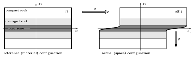
Figure 1: Schematic geometry of the fault zone in the material reference Lagrangian configuration (left) and the actual space Eulerian configuration deformed by a mapping $y\in H^{2}(\Omega;\mathbb{R}^{d})$ (right). The (possibly inhomogeneous) gravity force $g$ is prescribed naturally in the space configuration.

As effect of a deformation, the fault zone is sheared and damage is accumulated in a relatively narrow region (damage region) with a width of tens to hundreds of meters. Strains are mainly concentrated in the even narrower core zone, whose width ranges typically from centimeters to meters. The core can accommodate slips of the order of kilometers within millions of years [3]. This distinguished, multi-scale nature of fault dynamics can be tackled at different levels, ranging from the continuum-Euclidean (here meaning continuum mechanical or thermomechanical) description of the faults, to the granular description of fault structures and deformation fields, to the fractal nature of the fault network [3].

The focus of this contribution is on a description of seismic processes on faults by advancing a thermodynamically consistent model of large-strain dynamics in poroelastic rocks in terms of deformation, temperature, plastic and damage dynamics, and water content and porosity evolution. The model is detailed in Section 2 below and includes in particular the following main features:
$\ \circ$ Large-strain elastoplastic response combined with fast damage (rupture) and emission of seismic waves and their propagation. $\ \circ$ Flash heating: intense heat production during strong earthquakes influencing damage and sliding resistance, as in the Dieterich-Ruina friction model [15, 57], see also [53]. $\ \circ$ Modelization of saturated water flow and its influence on material response and eventually on earthquake dynamics [4]. $\ \circ$ Healing (also called aging) and gradual conversion of elastic strain to permanent inelastic deformation during long-lasting creep and material degradation.

The evolution in time of poroelastic rocks in upper lithospheric mantle are described as originating by the balance of energy-storage and dissipation mechanisms. In particular, we focus on a general form of free energy. This loses convexity upon damaging, as proposed in [41] and later used in several articles as, e.g. [24, 38, 39]. Such free energy is augmented by nonlocal energetics in form of a gradient damage and plastic theory [39, 36] and a strain gradient in the frame of so-called 2nd-grade nonsimple materials [18, 46, 58] (proposed under the name “materials with couple stresses” by R.A. Toupin [59]). Such materials are also known as weakly nonlocal. Nonlocal-material concepts have the capacity to be fitted with dispersion of elastic waves in general, cf. [30] for a thorough discussion. This effectively entails the control the scale of the damage and core regions. Eventually, the distinguished variational structure for the model allows allow for a comprehensive mathematical treatment, including existence of suitably-defined weak solutions, and convergence of a Galerkin approximation combined with a regularization.

With respect to previous geophysical modeling [37, 24, 38, 39, 36] the novelty of our contribution is threefold.
(i) Our model deals with large strains in a thermodynamically consistent way. This seems to move substantially forward with respect to the current literature, where description are either restricted to small strains or combines small elastic strains with large displacements (but not completely consistently, as noticed in [54]). The present model possesses a clear global energetics which can serve for a-priori estimates and rigorous analysis. (ii) By taking advantage of the variational nature of the model we are in the position of presenting a full coupling of effects. Mechanical and thermal evolution are consistently coupled with damage, porosity, and water content dynamics via the specification of the energy and dissipation potentials. Constitutive relations are directly defined in terms of variations of these potentials and combined with conservation of momenta and energy and internal dynamics. (iii) We derive a sound approximation and existence theory. In particular, we present a stable and convergent Galerkin-approximation scheme. This is unprecedented, to our knowledge, for such a comprehensive model at finite strains. One has to remark that the implementation of large-strain models is often computationally challenging in comparison to the small-strain models. Nevertheless, actual computations based on an updated Lagrangian scheme (see [12], for instance) may combine with the present model toward simulations. One has to mention that poroelastic models at large strains have already been considered from the engineering viewpoint, cf. [13, 8, 16, 19, 29], where nevertheless no rigorous analysis is addressed.

The plan of the paper is as follows. In Section 2 we formalize the model. In particular, we specify the form of the total energy and of the dissipation. This leads to the formulation of an evolution system of partial differential equations and inclusions. The thermodynamic consistency of the model and various possible modifications are also discussed. Section 3 presents a variational notion of solution as well as the main analytical statements. The existence proof via Galerkin’s approximation is then detailed in Section 4, with most technical mathematical arguments being related to the thermoviscoplasticity and just refer to [55]. Finally, Sect. 5 discusses some improvements of the model and related analytical complications.

2 Thermodynamical modeling

We devote this section to present our general model for damageable poroelastic continua with water and heat transfer. This is formulated in Lagrangian coordinates with $\Omega\subset\mathbb{R}^{d}$ ($d=2$ or $3$) being a bounded smooth reference (fixed) configuration. The variables of the model are

$$y:\Omega\to\mathbb{R}^{d}\quad$$ deformation,

$$\varPi:\Omega\to{\color[rgb]{0,0,0}^{+}(d)}$$ plastic part of the inelastic strain,

$$\alpha:\Omega\to\mathbb{R}\quad$$ damage descriptor (also called aging),

$$\phi:\Omega\to\mathbb{R}\quad \text{porosity (effectively the volumetric part of the inelastic strain)},$$

$$\zeta:\Omega\to[0,1]\quad$$ volume fraction of water,

$$\theta:\Omega\to(0,\infty)\quad$$ absolute temperature,

where ${\rm GL}^{+}(d)$ denotes the general linear group of matrices from $\mathbb{R}^{d\times d}$ with positive determinant. We emphasize that, although we have in mind saturated flows, we distinguish between water content and porosity. Indeed, compared to rocks, water is substantially compressible. Note that in the standard Biot model $\zeta\sim\phi$ can be achieved only asymptotically if $\beta=0$ and $m\to\infty$ in (1) below. Beside this interpretation, one can also think about a double-porosity model where the diffusant is transfered only by one system of pores.

For convenience, we anticipate in Table 1 the main notation, to be introduced in this section; for basic notions from continuum (thermo/poro)mechanics at large strains we refer e.g. to the monographs [1, 2, 13, 9, 11, 14, 21, 32]. In particular, note that $P$ is the rate of plastic strain in the intermediate configuration [43]. Here we should also note that we follow the terminological conventions in mechanics, which differs from what is used in engineering. In particular, we call stored energy all temperature-independent terms in the free energy.

$\Omega$ reference configuration, $\Gamma$ boundary of $\Omega$, $I:=[0,T]$ fixed time interval, $Q:=I{\times}\Omega$, $\Sigma:=I\times\Gamma$, $\varSigma_{\rm el}$ first Piola-Kirchhoff stress, $\varrho$ mass density (constant), $F=\nabla y$ deformation gradient, $F_{\rm el}$ elastic part of $F$, $E_{\rm el}$ elastic Green-Lagrange strain, $c_{\rm v}(\theta)$ heat capacity, $\text{\large$\mathbb{K}$}(\zeta,\theta)$ heat-conductivity tensor, $\mathscr{K}(\varPi,\phi,\zeta,\theta)$ pull-back of $\text{\large$\mathbb{K}$}(\zeta,\theta)$ $\vartheta$ rescaled temperature, $\eta$ entropy (per unit reference volume), $m=m(\alpha,\phi)$ Biot modulus, $\beta$ Biot coefficient, $\lambda=\lambda(\alpha,\phi)$ first Lamé coefficient, $G=G(\alpha,\phi)$ shear modulus, $p_{\rm por}$ pore pressure, $p_{\rm age}$ driving pressure for aging, $p_{\rm eff}$ driving pressure for porosity, $\psi$ free energy (in the reference configuration), $\psi_{{}_{\rm M}}$ mechanical part of $\psi$, $\psi_{{}_{\rm T}}$ thermal part of $\psi$, $\varSigma_{\rm in}$ driving stress for the plastification, $P$ a placeholder for plastic rate $\mathchoice{{\buildrel\hskip 0.90005pt\text{\LARGE.}\over{\varPi}}}{{\buildrel\hskip 0.90005pt\text{\Large.}\over{\varPi}}}{{\buildrel\hskip 0.90005pt\text{\large.}\over{\varPi}}}{{\buildrel\hskip 0.90005pt\text{\large.}\over{\varPi}}}\varPi^{-1}$, $\mathfrak{R}$ dissipation potential for plastification, $\mathfrak{D}$ dissipation potential for damage/porosity, $\gamma=\gamma(\alpha,\phi)$ non-Hookean elastic modulus, $\sigma=\sigma(\phi)$ porosity spherical strain influence, $r$ dissipated mechanical energy rate, $\text{\large$\mathbb{M}$}=\text{\large$\mathbb{M}$}(\alpha,\phi)$ hydraulic conductivity, $\mathscr{M}(\varPi,\alpha,\phi)$ pull-back of $\text{\large$\mathbb{M}$}(\alpha,\phi)$, $g$ gravity force in the actual space configuration, $y_{\flat}$ external displacement loading, $N$ constant of the elastic support, $\mu_{\flat}$ external chemical potential, $M$ permeability at the boundary, $K$ boundary heat-transfer coefficient, $\theta_{\flat}$ external temperature, $\chi$ specific stored energy of damage, $\kappa_{0}$, $\kappa_{1}$, $\kappa_{2}$, $\kappa_{3}$, $\kappa_{4}$ length-scale coefficients, $\tau_{\scriptscriptstyle\textrm{\rm rel}}$ relaxation time for chemical potential.

Table 1: Summary of the basic notation used through the paper.

The model will result by combining momentum and energy conservation with the dynamics of internal variables. In order to specify the latter and provide constitutive relations, we introduce a free energy and a dissipation (pseudo)potential in the following subsections.

2.1 Small-strain mechanical stored energy

A crucial novelty of the present modelization is that of dealing with finite strains. In order to motivate our assumptions on the mechanical stored energy in the coming Subsection 2.2, let us comment on a classical choice in the small-strain regime, namely

(1) $$\frac{1}{2}\lambda(\alpha)I_{1}^{2}+G(\alpha)I_{2}-\gamma(\alpha)I_{1}\sqrt{I_{2}}+\frac{1}{2}m|\beta I_{1}{-}\zeta{+}\phi|^{2}$$

with $\lambda(\alpha)=\lambda_{0},\ G(\alpha)=G_{0}-\alpha G_{\mathrm{r}},\ \gamma(\alpha)=\alpha\gamma_{\mathrm{r}}$, and with $I_{1}={\rm tr}\,e_{\rm el}$ and $I_{2}=|e_{\rm el}|^{2}$ and $e_{\rm el}$ denoting the elastic part of the small strain. When the undamaged-rock initial condition $\alpha_{0}=0$ is considered, the values $\lambda_{0}$ and $G_{0}$ are the initial values of the elastic moduli $\lambda(\alpha)$ and $G(\alpha)$ in the rock (disregarding porosity, which is later considered), while $G_{\mathrm{r}}>0$ and $\gamma_{\mathrm{r}}>0$ are suitable constants (in MPa). For $d=3$, the so-called strain invariant ratio $I_{1}\sqrt{I_{2}}$ varies from $-\sqrt{3}$ for isotropic compaction to $\sqrt{3}$ for isotropic dilation. The Biot $m$-term is an extension of the usual isotropic response of a Lamé material with constants $\lambda$ and $G$ (latter also called the shear modulus). Such extension was suggested in [4] and later augmented by the nonlinear (also called non-Hookean) $\gamma$-term in [5] at small strains. The special form of this last term was suggested in [40] (alternatively considered as $-\gamma I_{1}\sqrt{I_{2}{-}I_{1}^{2}/3}$ in [41]), validated, and used in series of works [23, 25, 34, 35, 38, 42]. The reader is referred to [26] for a comprehensive discussion on such choices.

Note that the above-introduced mechanical stored energy is 2-homogeneous in terms of $e_{\rm el}$ and that the function $\gamma$ in the $\gamma$-term makes it nonconvex if the damage parameter $\alpha$ is sufficiently large. This induces a loss of positive-definiteness of the Hessian of (1) which is intended to model the loss of stability of the rocks under damage, cf. [34]. From the mathematical standpoint, this feature makes the analysis challenging as both coercivity and monotonicity of the driving force fails. This seemingly prevents any rigorous existence theory even for short times, due to possible stress concentration. A possible way out from this obstruction was proposed in [54] by considering nonsimple materials and by a regularization of the stored energy. An analogous regularization will be here considered. Indeed, we will replace the term $\gamma(\alpha)I_{1}\sqrt{I_{2}}$ by a bounded term $\gamma(\alpha)I_{1}\sqrt{I_{2}}/(1{+}\epsilon I_{2})$ with a small, user-defined parameter $\epsilon>0$.

In the small-strain setting, the following additive decomposition of the total small strain is often considered

(2) $$e(u)=e_{\rm el}+e_{\rm pl}-\sigma(\phi)\mathbb{I}.$$

Here, $e_{\rm pl}$ is the trace-free plastic-strain tensor and $\sigma:[0,1]\to\mathbb{R}$ represents the pore volume (note that this is taken as $\sigma(\phi)=-\phi/3$ in [23, 38]). In [34], $e_{\rm pl}$ is eventually decomposed into the sum of a damage-related inelastic strain and a creep-induced ductile strain (with a Maxwellian viscosity of the order of $10^{22\pm 2}$Pa s), a distinction which we neglect here.

2.2 Mechanical stored energy

A focal point of our model is to move from the small to the finite strain situation. In particular, by replacing the small strain $e_{\rm el}$ with the elastic Green-Lagrange strain $E_{\rm el}=\frac{1}{2}(F_{\rm el}^{\top}F_{\rm el}-\mathbb{I})$, we correspondingly consider the mechanical stored energy (compare with (1)) as a function of the elastic strain $F_{\rm el}$ as

(3) $$\psi_{{}_{\rm M}} =\psi_{{}_{\rm M}}(F_{\rm el}{\color[rgb]{0,0,0},\varPi},\alpha,\phi,\zeta)=\frac{1}{2}\frac{\lambda(\alpha,\phi)I_{1}^{2}}{\sqrt[4]{1{+}\epsilon I_{2}}}+\frac{G(\alpha,\phi)I_{2}}{\sqrt[4]{1{+}\epsilon I_{2}}}-\gamma(\alpha,\phi)\frac{I_{1}\sqrt{I_{2}}}{1{+}\epsilon I_{2}}$$

$$\qquad\qquad\qquad\qquad\qquad{\color[rgb]{0,0,0}+\varpi(\det\varPi)}+\frac{1}{2}m(\alpha,\phi)\frac{|\beta I_{1}{-}\zeta{+}\phi|^{2}}{\sqrt[4]{1{+}\epsilon I_{2}}}+\chi(\alpha)$$

where now $I_{1}={\rm tr}\,E_{\rm el}$ and $I_{2}=|E_{\rm el}|^{2}$ with $E_{\rm el}=\displaystyle{\frac{F_{\rm el}^{\top}F_{\rm el}-\mathbb{I}}{2}}$ so that $I_{1}\sqrt{I_{2}}={\rm tr}\,E_{\rm el}|E_{\rm el}|$. The $\varpi$-term is a modelling ansatz to ensure the plastic deformation to be nearly isochoric, i.e. $\det\varPi\sim 1$. In combination with the plastic-gradient term, this ensures local invertibility of the plastic strain. Formally, such a term acting on $\varPi$ is in the position of isotropic hardening (typically occurring in metals). Such hardening effect is indeed not relevant in modelling of rocks or soils. It should be emphasized that, as here it controls only the volumetric part of $\varPi$, it does not cause any undesired hardening effects when plastifying the rocks in a isochoric way. The term $\chi(\alpha)$ in the right-hand side of (3) is the energy of damage and contributes an additional driving force for healing if $\chi^{\prime}>0$. The $\chi$-term can be microscopically interpreted as an extra energy contribution related with microvoids or microcracks, arising due to macroscopical damage. This term is indeed a stored energy, although if damage would be unidirectional (without healing), this energy would be effectively dissipated. Even in this case, however, it would not contribute to the heat production, differently from truly dissipative terms. Also let us note that, for $\epsilon=0$, (3) is an obvious analog of (1). Henceforth, we will however stick with a small but fixed $\epsilon>0$ in (3). This yields a 3rd-order polynomial growth of $\psi_{{}_{\rm M}}$ with respect to $F_{\rm el}$, which in turn ensures that its derivative has a 2nd-order polynomial growth. In particular, all driving forces of the system, to be defined in (8b,d) below, will turn out to belong to $L^{2}$ spaces. Before moving on, let us remark that the above choice of $\psi_{{}_{\rm M}}$ could be generalized, as long as growth and smoothness properties are conserved. We shall however stick to (3) for the sake of comparison with the small-strain theory.

A possible choice for the dependence of the nonlinearities in (3) is

(4a) $$\lambda(\alpha,\phi)=(\lambda_{0}-\alpha\lambda_{\rm r})\big{(}1{-}\phi/\phi_{\rm cr}\big{)},\ \ \ \$$

(4b) $$G(\alpha,\phi)=\big{(}G_{0}-\alpha G_{\mathrm{r}}\big{)}\big{(}1{-}\phi/\phi_{\rm cr}\big{)},\ \ \ \$$

(4c) $$\gamma(\alpha,\phi)=\alpha\gamma_{\mathrm{r}}\big{(}1{-}\phi/\phi_{\rm cr}\big{)},\ \ \ \$$

(4d) $$m(\alpha,\phi)=\alpha m_{0}\big{(}1{-}\phi/\phi_{\rm cr}\big{)},$$

cf. [23, 38], where $\phi_{\rm cr}$ denotes the porosity upper bound in which the material loses its stiffness. A typical value of $\phi_{\rm cr}$ used in geophysical applications is rather high, strong sandstones (e.g. Berea) may be $\sim$20% while in other rocks it migh be even 30% or 40%. As for $\chi(\cdot)$, this direct damage energy is not considered in the mentioned geophysical literature but it has a clear interpretation (as already explained) and may be a reasonable source of healing in addition to that healing due to $-\alpha\lambda_{\rm r}$ and $-\alpha G_{\mathrm{r}}$ terms in (4a,b). Besides, this term may also contribute to localization of damaged regions, which is routinely used in fracture mechanics under the name a “phase-field fracture”. In the case of an undamaged nonporous rock (i.e. $\epsilon=\alpha=\phi=0$ so that $\gamma(\alpha,\phi)=m(\alpha,\phi)=\chi(\alpha)=0$ as well), the mechanical stored energy (3) reduces to ${\lambda_{0}}({\rm tr}E_{\rm el})^{2}/2+G_{0}|E_{\rm el}|^{2}$, namely to the classical St. Venant-Kirchhoff material. As $\psi_{{}_{\rm M}}$ depends on the elastic Cauchy-Green tensor $F_{\rm el}^{\top}F_{\rm el}$ and $\varPi^{\top}\varPi$ rather than on $F_{\rm el}$ and $\varPi$, so that the mechanical energy is both frame- and plastic-indifferent, namely

(5) $$\forall R_{1},{\color[rgb]{0,0,0}R_{2}}\in{\rm SO}(d):\ \ \psi_{{}_{\rm M}}(R_{1}F_{\rm el}{\color[rgb]{0,0,0},R_{2}\varPi},\alpha,\phi,\zeta)=\psi_{{}_{\rm M}}(F_{\rm el}{\color[rgb]{0,0,0},\varPi},\alpha,\phi,\zeta),$$

Here, we used the notation ${\rm SO}(d)$ for the matrix group ${\rm SO}(d):=\{{\color[rgb]{0,0,0}R}\in\mathbb{R}^{d\times d},\ {\color[rgb]{0,0,0}RR}^{\top}={\color[rgb]{0,0,0}R}^{\top}{\color[rgb]{0,0,0}R}=\mathbb{I},\ \det{\color[rgb]{0,0,0}R}=1\}$ where the superscript $\top$ stands for transposition and $\mathbb{I}$ is the identity matrix.

The additive decomposition (2) from the small-strain case is no longer available and one has to replace it with the standard Kröner-Lee-Liu multiplicative decomposition [31, 33]

(6) $$F=F_{\rm el}\varPi S\ \ \text{ with }F=\nabla y\ \text{ and }\ S=S(\phi)=\mathbb{I}/\sigma(\phi).$$

Here, the nonlinearity $\sigma=\sigma(\phi)$ is related to the stress-free isotropic shrinkage of the specimen at given porosity $\phi$. This corresponds to an expansion of volume $1/\sigma^{d}(\phi)$-times in the stress-free state; note that $\det F=(\det F_{\rm el})(\det\varPi)/\sigma^{d}(\phi)\sim 1/\sigma^{d}(\phi)$ because $\det\varPi\sim 1$ and also $\det F_{\rm el}\sim 1$ since $E_{\rm el}$ is assumed small so that $\det F_{\rm el}=\det(F_{\rm el}^{\top}F_{\rm el})^{1/2}=\det(2E_{\rm el}+\mathbb{I})^{1/2}\sim(\det\mathbb{I})^{1/2}=1$. Using $\sigma(\phi)$ in the position of shrinkage rather than expansion in (6) corresponds to the negative sign in (2) and gives a simpler formula because $\sigma(\theta)$ occurs in $F_{\rm el}$ instead of $1/\sigma(\theta)$. Our basic modeling assumption simplifying the model as far as the formulation and the analysis (cf. also Sect. 5) is that the elastic part of the Green-Lagrange strain is small, namely ${\color[rgb]{0,0,0}E_{\rm el}=\frac{1}{2}(F_{\rm el}^{\top}F_{\rm el}-\mathbb{I})\sim 0}$, and, correspondingly, large deformations are accommodated by the inelastic term. Yet, the large rotations are naturally allowed, so we do not assume directly $\nabla y\sim\varPi S$ which might be too restrictive in some geophysically relevant situations.

In addition to the already mentioned nonconvex $\gamma$-term, the geometrically nonlinear setting of (6) induces additional nonconvexity of $\psi_{{}_{\rm M}}$. On the other hand, note that $\psi_{{}_{\rm M}}$ is strongly convex in terms of the water content $\zeta$. This makes the model amenable to a mathematical discussion even without considering nonlocal contributions (gradient terms) for $\zeta$, which would lead to the Cahn-Hilliard dynamics. This feature will be used later in order to deduce the strong convergence of the gradient of the chemical potential (i.e. of the pore pressure).

The multiplicative decomposition (6) allows to express the free energy in terms of the total strain tensor and inelastic/ductile strains via the substitution $F_{\rm el}=F\varPi^{-1}S^{-1}(\phi){\color[rgb]{0,0,0}=\sigma(\phi)F\varPi^{-1}}$. In addition, the mechanical stored energy will be augmented by gradient terms and a thermal contribution $\psi_{{}_{\rm T}}$ (considered for simplicity to depend solely on temperature, i.e., thermal expansion which is not a dominant effect in geophysical models is here neglected). By integrating over the reference configuration $\Omega$ with $F=\nabla y$, the total free energy of the body is expressed by

(7) $$\Psi(\nabla y,\varPi,\alpha,\phi,\zeta,\theta)=\Psi_{{}_{\rm M}}(\nabla y,\varPi,\alpha,\phi,\zeta)+\Psi_{{}_{\rm T}}(\theta)$$

$$\ \ \ \text{ with }\ \Psi_{{}_{\rm T}}(\theta)=\int_{\Omega}\!\psi_{{}_{\rm T}}(\theta)\,{\rm d}x$$

$$\ \ \ \text{ and }\ \ \Psi_{{}_{\rm M}}(\nabla y,\varPi,\alpha,\phi,\zeta)=\int_{\Omega}\psi_{{}_{\rm M}}(\sigma(\phi)\nabla y\,{\color[rgb]{0,0,0}\varPi^{-1}}\!{\color[rgb]{0,0,0},\varPi},\alpha,\phi,\zeta)+\frac{1}{2}\kappa_{0}\big{|}\nabla^{2}y\big{|}^{2}$$

$$\hskip 30.00005pt+\frac{1}{q}\kappa_{1}|\nabla\varPi|^{q}+\frac{1}{2}\kappa_{2}|\nabla\alpha|^{2}+\frac{1}{2}\kappa_{3}|\nabla\phi|^{2}+\frac{1}{2}\kappa_{4}|\nabla\zeta|^{2}+\delta_{[0,1]}(\zeta)\,{\rm d}x,$$

where additional gradient terms are considered. In particular, the $\kappa_{0}$-term qualifies the material as 2nd-grade nonsimple, also called multipolar or complex, see the seminal [59] and [18, 45, 46, 48, 58, 60]. The exponent $q$ in the $\kappa_{1}$-term is given and fixed to be larger than $d$, which eases some points of the analysis. Note however that the choice $\kappa_{1}(\nabla\varPi)|\nabla\varPi|^{2}$ for some $\kappa_{1}(\nabla\varPi)\sim 1+|\nabla\varPi|^{q-2}$ could be considered as well. The gradient terms in $\alpha$, $\phi$, and $\zeta$ are intended to describe nonlocal effects and effectively encode the emergence of length scales associated with damage, porosity, and water-content profiles, respectively.

The symbol $\delta_{[0,1]}(\cdot)$ denotes the indicator function $\delta_{[0,1]}(\zeta)=0$ if $0\leq\zeta\leq 1$ and $\delta_{[0,1]}(\zeta)=\infty$ elsewhere. This indicator function encodes the constraint $0\leq\zeta\leq 1$. The frame- and plastic-indifference of the mechanical stored energy (5) translates in terms of $\Psi$ as

$$\forall R_{1},{\color[rgb]{0,0,0}R_{2}}\in{\rm SO}(d):\ \ \Psi({R_{1}}\nabla y,{\color[rgb]{0,0,0}R_{2}}\varPi,\alpha,\phi,\zeta,\theta)=\Psi(\nabla y,\varPi,\alpha,\phi,\zeta,\theta).$$

In particular let us note that the gradient terms are frame-indifferent as well.

The partial functional derivatives of $\Psi$ give origin to corresponding driving forces. We use the symbol $\partial_{w}$ to indicate both differentiation with respect to the variable $w$ of a smooth function or functional or subdifferentiation of a convex function or functional. The second Piola-Kirchhoff stress $\varSigma_{\rm el}$, here augmented by a contribution arising from the gradient $\kappa_{0}$-term, is defined as

(8a) $$\varSigma_{\rm el}=\partial_{\nabla y}\Psi=\sigma(\phi)\partial_{F_{\rm el}}\psi_{{}_{\rm M}}(\sigma(\phi)\nabla y{\color[rgb]{0,0,0}\varPi^{-1}}\!,\alpha,\phi,\zeta){\color[rgb]{0,0,0}\varPi^{-T}}-\kappa_{0}{\rm div}\nabla^{2}y.\ \ \ \$$

Furthermore, the driving stress for the plastification, again involving a contribution arising from the gradient $$\kappa_{1}$$-term, reads

(8b) $$\varSigma_{\rm in}=\partial_{\varPi}\Psi=\sigma(\phi)\nabla y^{\top}\partial_{F_{\rm el}}\psi_{{}_{\rm M}}(\sigma(\phi)\nabla y{\color[rgb]{0,0,0}\varPi^{-1}}\!,\alpha,\phi,\zeta):\partial_{\varPi}{\color[rgb]{0,0,0}\varPi^{-1}}$$

$$\hskip 140.00021pt{\color[rgb]{0,0,0}+\varpi^{\prime}(\det\varPi){\color[rgb]{0,0,0}\varPi^{-T}}}-{\rm div}(\kappa_{1}|\nabla\varPi|^{q-2}\nabla\varPi).$$

Here and in the following we use the (standard) notation “$$\,\cdot\, \,:\, \,\vdots\, \partial_{\varPi}{\color[rgb]{0,0,0}\varPi^{-1}} \sigma(\phi)\nabla y^{\top}\partial_{F_{\rm el}}\psi_{{}_{\rm M}}(\sigma(\phi)\nabla y{\color[rgb]{0,0,0}\varPi^{-1}}\!,\alpha,\phi,\zeta):\partial_{\varPi}{\color[rgb]{0,0,0}\varPi^{-1}}$$” and “” and “” for the contraction product of vectors, 2nd-order, and 3rd tensors, respectively. As is a 4th-order tensor, the product turns out to be a 2nd-order tensor, as expected. The thermodynamical driving pressure for damage is

(8c) $$p_{\rm age}=\partial_{\alpha}\Psi=\partial_{\alpha}\psi_{{}_{\rm M}}(\sigma(\phi)\nabla y{\color[rgb]{0,0,0}\varPi^{-1}}\!,\alpha,\phi,\zeta)-\kappa_{2}\Delta\alpha,$$

and the driving force for porosity-evolution (a so-called effective pressure) is

(8d) $$p_{\rm eff}=\partial_{\phi}\Psi={\rm tr}\big{(}\sigma^{\prime}(\phi){\color[rgb]{0,0,0}\varPi^{-T}}\nabla y^{\top}\partial_{F_{\rm el}}\psi_{{}_{\rm M}}(\sigma(\phi)\nabla y{\color[rgb]{0,0,0}\varPi^{-1}}\!,\alpha,\phi,\zeta)\big{)}$$

$$\hskip 58.0001pt+\partial_{\phi}\psi_{{}_{\rm M}}(\sigma(\phi)\nabla y{\color[rgb]{0,0,0}\varPi^{-1}}\!,\alpha,\phi,\zeta)-\kappa_{3}\Delta\phi.$$

Analogously, we also identify the pore pressure $$p_{\rm por}$$ as

(8e) $$p_{\rm por}\in\partial_{\zeta}\Psi=\partial_{\zeta}\psi_{{}_{\rm M}}(\sigma(\phi)\nabla y{\color[rgb]{0,0,0}\varPi^{-1}}\!,\alpha,\phi,\zeta)-\kappa_{4}\Delta\zeta+\mathfrak{N}_{[0,1]}(\zeta)$$

$$\hskip 48.00009pt=m(\alpha,\phi)\frac{\zeta{-}\phi{-}\beta I_{1}}{\sqrt[4]{1{+}\epsilon I_{2}}}-\kappa_{4}\Delta\zeta+\mathfrak{N}_{[0,1]}(\zeta),$$

where $\mathfrak{N}_{[0,1]}(\zeta)$ is the normal cone to the interval $[0,1]$ at $\zeta$. All variations of $\Psi$ above are taken with respect to the corresponding $L^{2}$ topologies.

2.3 Thermodynamical system

The entropy $\eta$, the heat capacity $c_{\rm v}$, and the thermal part $\vartheta$ of the internal energy (per unit reference volume) are classically recovered as

(9) $$\eta=-\psi_{\theta}^{\prime}=-\psi_{{}_{\rm T}}^{\prime}(\theta),\ \ \ \ c_{\rm v}=-\theta\psi_{\theta\theta}^{\prime\prime}=-\theta\psi_{{}_{\rm T}}^{\prime\prime}(\theta),\ \ \text{ and }\ \ \vartheta=\psi_{{}_{\rm T}}(\theta)-\theta\psi_{{}_{\rm T}}^{\prime}(\theta).$$

Note in particular that $\mathchoice{{\buildrel\hskip 1.00006pt\text{\LARGE.}\over{\vartheta}}}{{\buildrel\hskip 1.00006pt\text{\Large.}\over{\vartheta}}}{{\buildrel\hskip 1.00006pt\text{\large.}\over{\vartheta}}}{{\buildrel\hskip 1.00006pt\text{\large.}\over{\vartheta}}}=\psi_{{}_{\rm T}}^{\prime}(\theta)\mathchoice{{\buildrel\hskip 1.00006pt\text{\LARGE.}\over{\theta}}}{{\buildrel\hskip 1.00006pt\text{\Large.}\over{\theta}}}{{\buildrel\hskip 1.00006pt\text{\large.}\over{\theta}}}{{\buildrel\hskip 1.00006pt\text{\large.}\over{\theta}}}-\mathchoice{{\buildrel\hskip 1.00006pt\text{\LARGE.}\over{\theta}}}{{\buildrel\hskip 1.00006pt\text{\Large.}\over{\theta}}}{{\buildrel\hskip 1.00006pt\text{\large.}\over{\theta}}}{{\buildrel\hskip 1.00006pt\text{\large.}\over{\theta}}}\psi_{{}_{\rm T}}^{\prime}(\theta)-\theta\psi_{{}_{\rm T}}^{\prime\prime}(\theta)\mathchoice{{\buildrel\hskip 1.00006pt\text{\LARGE.}\over{\theta}}}{{\buildrel\hskip 1.00006pt\text{\Large.}\over{\theta}}}{{\buildrel\hskip 1.00006pt\text{\large.}\over{\theta}}}{{\buildrel\hskip 1.00006pt\text{\large.}\over{\theta}}}=c_{\rm v}(\theta)\mathchoice{{\buildrel\hskip 1.00006pt\text{\LARGE.}\over{\theta}}}{{\buildrel\hskip 1.00006pt\text{\Large.}\over{\theta}}}{{\buildrel\hskip 1.00006pt\text{\large.}\over{\theta}}}{{\buildrel\hskip 1.00006pt\text{\large.}\over{\theta}}}$. The entropy equation reads as

(10) $$\theta\mathchoice{{\buildrel\hskip 1.00006pt\text{\LARGE.}\over{\eta}}}{{\buildrel\hskip 1.00006pt\text{\Large.}\over{\eta}}}{{\buildrel\hskip 1.00006pt\text{\large.}\over{\eta}}}{{\buildrel\hskip 1.00006pt\text{\large.}\over{\eta}}}+{\rm div}\,j=\text{dissipation rate}.$$

We assume the heat flux $j$ to be governed by the Fourier law $j=-\mathscr{K}\nabla\theta$ where is $\mathscr{K}$ the heat-conductivity tensor. Substituting $\eta$ from (9) into (10), we arrive at the heat-transfer equation

$$c_{\rm v}(\theta)\mathchoice{{\buildrel\hskip 1.00006pt\text{\LARGE.}\over{\theta}}}{{\buildrel\hskip 1.00006pt\text{\Large.}\over{\theta}}}{{\buildrel\hskip 1.00006pt\text{\large.}\over{\theta}}}{{\buildrel\hskip 1.00006pt\text{\large.}\over{\theta}}}-{\rm div}(\mathscr{K}\nabla\theta)=\text{dissipation rate}.$$

Note that, $c_{\rm v}$ depends of temperature only as so does $\psi_{{}_{\rm T}}$.

The water-content gradient (i.e. the $\kappa_{4}$-term) describes capillarity effects and it is standardly referred to as the Cahn-Hilliard model [7], $\mu$ is the chemical potential and (8e) corresponds to diffusion governed by the (generalized) Fick-Darcy law. Note that this simplified model for a stiff poroelastic matrix interacting with a moving fluid is largely accepted in the geophysical context [49]. In order to cope with the direct coupling of $\zeta$ with $\theta$ in (1), we consider some viscous dynamics, following the original Gurtin’s ideas [22], cf. also [6, 17, 20, 28, 50]. This involves some relaxation time $\tau_{\scriptscriptstyle\textrm{\rm rel}}>0$ and a contribution $\tau_{\scriptscriptstyle\textrm{\rm rel}}\mathchoice{{\buildrel\hskip 1.00006pt\text{\LARGE.}\over{\zeta}}}{{\buildrel\hskip 1.00006pt\text{\Large.}\over{\zeta}}}{{\buildrel\hskip 1.00006pt\text{\large.}\over{\zeta}}}{{\buildrel\hskip 1.00006pt\text{\large.}\over{\zeta}}}^{2}$ to the dissipation rate.

In summary, the model consists of a system of semilinear equations of the form

(11a) $$\varrho\mathchoice{{\buildrel\hskip 1.30005pt\text{\LARGE..}\over{y}}}{{\buildrel\hskip 1.00006pt\text{\Large..}\over{y}}}{{\buildrel\hskip 1.00006pt\text{\large..}\over{y}}}{{\buildrel\hskip 1.00006pt\text{\large..}\over{y}}}={\rm div}\,\varSigma_{\rm el}+g(y),\!\!$$ (momentum equilibrium)

(11b) $$\partial_{P}\mathfrak{R}\big{(}\alpha,\phi,\theta;\mathchoice{{\buildrel\hskip 1.00006pt\text{\LARGE.}\over{\varPi}}}{{\buildrel\hskip 1.00006pt\text{\Large.}\over{\varPi}}}{{\buildrel\hskip 1.00006pt\text{\large.}\over{\varPi}}}{{\buildrel\hskip 1.00006pt\text{\large.}\over{\varPi}}}\varPi^{-1}\big{)}+\,\varSigma_{\rm in}\varPi^{\top}=0,$$ (flow rule for inelastic strain)

(11i) $$\partial_{(\mathchoice{{\buildrel\hskip 0.70004pt\text{\LARGE.}\over{\alpha}}}{{\buildrel\hskip 0.70004pt\text{\Large.}\over{\alpha}}}{{\buildrel\hskip 0.70004pt\text{\large.}\over{\alpha}}}{{\buildrel\hskip 0.70004pt\text{\large.}\over{\alpha}}},\mathchoice{{\buildrel\hskip 0.70004pt\text{\LARGE.}\over{\phi}}}{{\buildrel\hskip 0.70004pt\text{\Large.}\over{\phi}}}{{\buildrel\hskip 0.70004pt\text{\large.}\over{\phi}}}{{\buildrel\hskip 0.70004pt\text{\large.}\over{\phi}}})}\mathfrak{D}\Big{(}\!\alpha,\phi,\theta;\Big{(}\!\begin{array}[]{c}\mathchoice{{\buildrel\hskip 1.00006pt\text{\LARGE.}\over{\alpha}}}{{\buildrel\hskip 1.00006pt\text{\Large.}\over{\alpha}}}{{\buildrel\hskip 1.00006pt\text{\large.}\over{\alpha}}}{{\buildrel\hskip 1.00006pt\text{\large.}\over{\alpha}}}\\[-3.00003pt] \mathchoice{{\buildrel\hskip 1.00006pt\text{\LARGE.}\over{\phi}}}{{\buildrel\hskip 1.00006pt\text{\Large.}\over{\phi}}}{{\buildrel\hskip 1.00006pt\text{\large.}\over{\phi}}}{{\buildrel\hskip 1.00006pt\text{\large.}\over{\phi}}}\end{array}\!\Big{)}\Big{)}+\Big{(}\!\!\begin{array}[]{c}p_{\rm age}\!\\[-1.00006pt] p_{\rm eff}\end{array}\!\!\Big{)}=\Big{(}\!\!\begin{array}[]{c}0\!\!\\[-1.00006pt] 0\!\!\end{array}\Big{)},\!\!$$ (flow rule for damage/porosity)

(11j) $$\mathchoice{{\buildrel\hskip 1.00006pt\text{\LARGE.}\over{\zeta}}}{{\buildrel\hskip 1.00006pt\text{\Large.}\over{\zeta}}}{{\buildrel\hskip 1.00006pt\text{\large.}\over{\zeta}}}{{\buildrel\hskip 1.00006pt\text{\large.}\over{\zeta}}}=\color[rgb]{0,0,0}\big{(}\mathscr{M}(\varPi,\alpha,\phi)\nabla\mu\big{)},$$ (water-transport equation)

(11k) $$\mu=p_{\rm por}+\tau_{\scriptscriptstyle\textrm{\rm rel}}\mathchoice{{\buildrel\hskip 1.00006pt\text{\LARGE.}\over{\zeta}}}{{\buildrel\hskip 1.00006pt\text{\Large.}\over{\zeta}}}{{\buildrel\hskip 1.00006pt\text{\large.}\over{\zeta}}}{{\buildrel\hskip 1.00006pt\text{\large.}\over{\zeta}}},$$ (equation for chemical potential)

(11l) $$c_{\rm v}(\theta)\mathchoice{{\buildrel\hskip 1.00006pt\text{\LARGE.}\over{\theta}}}{{\buildrel\hskip 1.00006pt\text{\Large.}\over{\theta}}}{{\buildrel\hskip 1.00006pt\text{\large.}\over{\theta}}}{{\buildrel\hskip 1.00006pt\text{\large.}\over{\theta}}}={\rm div}\big{(}\mathscr{K}(\varPi,\phi,\zeta,\theta)\nabla\theta\big{)}+r\!\!$$ (heat-transfer equation)

(11m) $$\qquad\text{with }\ r=r\big{(}\varPi,\alpha,\phi,\theta;\mathchoice{{\buildrel\hskip 1.00006pt\text{\LARGE.}\over{\varPi}}}{{\buildrel\hskip 1.00006pt\text{\Large.}\over{\varPi}}}{{\buildrel\hskip 1.00006pt\text{\large.}\over{\varPi}}}{{\buildrel\hskip 1.00006pt\text{\large.}\over{\varPi}}},\mathchoice{{\buildrel\hskip 1.00006pt\text{\LARGE.}\over{\alpha}}}{{\buildrel\hskip 1.00006pt\text{\Large.}\over{\alpha}}}{{\buildrel\hskip 1.00006pt\text{\large.}\over{\alpha}}}{{\buildrel\hskip 1.00006pt\text{\large.}\over{\alpha}}},\mathchoice{{\buildrel\hskip 1.00006pt\text{\LARGE.}\over{\phi}}}{{\buildrel\hskip 1.00006pt\text{\Large.}\over{\phi}}}{{\buildrel\hskip 1.00006pt\text{\large.}\over{\phi}}}{{\buildrel\hskip 1.00006pt\text{\large.}\over{\phi}}},\mathchoice{{\buildrel\hskip 1.00006pt\text{\LARGE.}\over{\zeta}}}{{\buildrel\hskip 1.00006pt\text{\Large.}\over{\zeta}}}{{\buildrel\hskip 1.00006pt\text{\large.}\over{\zeta}}}{{\buildrel\hskip 1.00006pt\text{\large.}\over{\zeta}}},\nabla\mu\big{)}$$

(11r) $$\hskip 50.00008pt=\partial_{P}\mathfrak{R}\big{(}\alpha,\phi,\theta;\mathchoice{{\buildrel\hskip 1.00006pt\text{\LARGE.}\over{\varPi}}}{{\buildrel\hskip 1.00006pt\text{\Large.}\over{\varPi}}}{{\buildrel\hskip 1.00006pt\text{\large.}\over{\varPi}}}{{\buildrel\hskip 1.00006pt\text{\large.}\over{\varPi}}}\varPi^{-1}){:}(\mathchoice{{\buildrel\hskip 1.00006pt\text{\LARGE.}\over{\varPi}}}{{\buildrel\hskip 1.00006pt\text{\Large.}\over{\varPi}}}{{\buildrel\hskip 1.00006pt\text{\large.}\over{\varPi}}}{{\buildrel\hskip 1.00006pt\text{\large.}\over{\varPi}}}\varPi^{-1})+\partial_{(\mathchoice{{\buildrel\hskip 0.70004pt\text{\LARGE.}\over{\alpha}}}{{\buildrel\hskip 0.70004pt\text{\Large.}\over{\alpha}}}{{\buildrel\hskip 0.70004pt\text{\large.}\over{\alpha}}}{{\buildrel\hskip 0.70004pt\text{\large.}\over{\alpha}}},\mathchoice{{\buildrel\hskip 0.70004pt\text{\LARGE.}\over{\phi}}}{{\buildrel\hskip 0.70004pt\text{\Large.}\over{\phi}}}{{\buildrel\hskip 0.70004pt\text{\large.}\over{\phi}}}{{\buildrel\hskip 0.70004pt\text{\large.}\over{\phi}}})}\mathfrak{D}\Big{(}\alpha,\phi,\theta;\Big{(}\!\begin{array}[]{c}\mathchoice{{\buildrel\hskip 1.00006pt\text{\LARGE.}\over{\alpha}}}{{\buildrel\hskip 1.00006pt\text{\Large.}\over{\alpha}}}{{\buildrel\hskip 1.00006pt\text{\large.}\over{\alpha}}}{{\buildrel\hskip 1.00006pt\text{\large.}\over{\alpha}}}\\[-1.00006pt] \mathchoice{{\buildrel\hskip 1.00006pt\text{\LARGE.}\over{\phi}}}{{\buildrel\hskip 1.00006pt\text{\Large.}\over{\phi}}}{{\buildrel\hskip 1.00006pt\text{\large.}\over{\phi}}}{{\buildrel\hskip 1.00006pt\text{\large.}\over{\phi}}}\end{array}\!\Big{)}\Big{)}{\cdot}\Big{(}\!\begin{array}[]{c}\mathchoice{{\buildrel\hskip 1.00006pt\text{\LARGE.}\over{\alpha}}}{{\buildrel\hskip 1.00006pt\text{\Large.}\over{\alpha}}}{{\buildrel\hskip 1.00006pt\text{\large.}\over{\alpha}}}{{\buildrel\hskip 1.00006pt\text{\large.}\over{\alpha}}}\\[-1.00006pt] \mathchoice{{\buildrel\hskip 1.00006pt\text{\LARGE.}\over{\phi}}}{{\buildrel\hskip 1.00006pt\text{\Large.}\over{\phi}}}{{\buildrel\hskip 1.00006pt\text{\large.}\over{\phi}}}{{\buildrel\hskip 1.00006pt\text{\large.}\over{\phi}}}\end{array}\!\Big{)}$$

$$\hskip 50.00008pt+\tau_{\scriptscriptstyle\textrm{\rm rel}}\mathchoice{{\buildrel\hskip 1.00006pt\text{\LARGE.}\over{\zeta}}}{{\buildrel\hskip 1.00006pt\text{\Large.}\over{\zeta}}}{{\buildrel\hskip 1.00006pt\text{\large.}\over{\zeta}}}{{\buildrel\hskip 1.00006pt\text{\large.}\over{\zeta}}}^{2}+\mathscr{M}(\varPi,\alpha,\phi)\nabla\mu{\cdot}\nabla\mu,$$ (heat-production rate)

where $\mathfrak{R}=\mathfrak{R}\big{(}\alpha,\phi,\theta;P)$ is the pseudopotential related to dissipative forces of visco-plastic origin ($P$ is the placeholder for the rate of plastic strain $\mathchoice{{\buildrel\hskip 1.00006pt\text{\LARGE.}\over{\varPi}}}{{\buildrel\hskip 1.00006pt\text{\Large.}\over{\varPi}}}{{\buildrel\hskip 1.00006pt\text{\large.}\over{\varPi}}}{{\buildrel\hskip 1.00006pt\text{\large.}\over{\varPi}}}\varPi^{-1}$), and $\mathfrak{D}(\alpha,\phi,\theta;\cdot)$ is the dissipation potential related to damage and porosity evolution.

The effective transport matrices $\mathscr{K}$ and $\mathscr{M}$ are to be related with the hydraulic-conductivity and the heat-conductivity symmetric tensors $\text{\large$\mathbb{M}$}=\text{\large$\mathbb{M}$}(\alpha,\phi)$ and $\text{\large$\mathbb{K}$}=\text{\large$\mathbb{K}$}(\zeta,\theta)$ which are given material properties. The need for such effective quantities stems form the fact that driving forces are to be considered Eulerian in nature, so that a pull-back to the reference configuration is imperative. A first choice would then be

(12a) $$\mathscr{M}(F,\alpha,\phi) =(\det F)F^{-\top}\text{\large$\mathbb{M}$}(\alpha,\phi)F^{-1}=(\mathrm{Cof}F)\text{\large$\mathbb{M}$}(\alpha,\phi)F^{-1}=\frac{1}{{\det F}}(\mathrm{Cof}F)\text{\large$\mathbb{M}$}(\alpha,\phi)\mathrm{Cof}F^{\top}$$

(12b) $$\mathscr{K}(F,\zeta,\theta) =\frac{1}{{\det F}}{(\mathrm{Cof}F)\text{\large$\mathbb{K}$}(\zeta,\theta)\mathrm{Cof}F^{\top}}.$$

These are just usual pull-back transformations of 2nd-order covariant tensors, cf. also Remark 2.2 below for some more discussion. Let us recall that our modeling assumption is that $E_{\rm el}$ is small so that $F^{\top}F\sim S^{\top}(\phi)\varPi^{\top}\varPi S(\phi)=\varPi^{\top}\varPi/\sigma^{2}(\phi)$. Thus, by replacing $F$ by $\varPi S(\phi)=\varPi/\sigma(\phi)$ (see Remark 2.3 below for some more discussion) and using the specific homogeneity of the determinant and the cofactor, relations (12) can be rewritten as

(13a) $$\mathscr{M}(\varPi,\alpha,\phi)\ =\ \sigma(\phi)^{2-d}\frac{{\color[rgb]{0,0,0}\varPi^{-T}}\text{\large$\mathbb{M}$}(\alpha,\phi){\color[rgb]{0,0,0}\varPi^{-1}}}{{\color[rgb]{0,0,0}\det\varPi}},$$

(13b) $$\mathscr{K}(\varPi,\zeta,\theta)\ =\ \sigma(\phi)^{2-d}\frac{{\color[rgb]{0,0,0}\varPi^{-T}}\text{\large$\mathbb{K}$}(\zeta,\theta){\color[rgb]{0,0,0}\varPi^{-1}}}{{\color[rgb]{0,0,0}\det\varPi}}.$$

These expressions bear the advantage of being independent of $(\nabla y)^{-1}$, which turns out useful in relation with estimation and passage to the limit arguments, cf. [32, 56].

Note that the right-hand side of (11a) features the pull-back $g{\circ}y$ of the actual gravity force $g:\mathbb{R}^{d}\to\mathbb{R}^{d}$. This allows us to consider a spatially inhomogoneous gravity, a generality which could turn out to be sensible at geophysical scales.

The plastic flow rule (11b) complies with the so-called plastic-indifference requirement. Indeed, the evolution is insensitive to prior plastic deformations, for the stored energy and the dissipation potential

$$\widehat{\psi}_{{}_{\rm M}}(F,\varPi,\alpha,\phi,\zeta):=\psi_{{}_{\rm M}}(F_{\rm el},\alpha,\phi,\zeta)\ \ \ \ \text{ and }\ \ \ \ \widehat{\mathfrak{R}}(\varPi,\alpha,\phi,\theta;\mathchoice{{\buildrel\hskip 1.00006pt\text{\LARGE.}\over{\varPi}}}{{\buildrel\hskip 1.00006pt\text{\Large.}\over{\varPi}}}{{\buildrel\hskip 1.00006pt\text{\large.}\over{\varPi}}}{{\buildrel\hskip 1.00006pt\text{\large.}\over{\varPi}}})=\mathfrak{R}(\alpha,\phi,\theta;\mathchoice{{\buildrel\hskip 1.00006pt\text{\LARGE.}\over{\varPi}}}{{\buildrel\hskip 1.00006pt\text{\Large.}\over{\varPi}}}{{\buildrel\hskip 1.00006pt\text{\large.}\over{\varPi}}}{{\buildrel\hskip 1.00006pt\text{\large.}\over{\varPi}}}\varPi^{-1})$$

respect the invariances $\widehat{\psi}_{{}_{\rm M}}(F\widetilde{\varPi},\varPi\widetilde{\varPi},\alpha,\phi,\zeta)=\widehat{\psi}_{{}_{\rm M}}(F,\varPi,\alpha,\phi,\zeta)$ and $\widehat{\mathfrak{R}}(\varPi\widetilde{\varPi},\alpha,\phi,\theta;\mathchoice{{\buildrel\hskip 1.00006pt\text{\LARGE.}\over{\varPi}}}{{\buildrel\hskip 1.00006pt\text{\Large.}\over{\varPi}}}{{\buildrel\hskip 1.00006pt\text{\large.}\over{\varPi}}}{{\buildrel\hskip 1.00006pt\text{\large.}\over{\varPi}}}\widetilde{\varPi})=\widehat{\mathfrak{R}}(\varPi,\alpha,\phi,\theta;\mathchoice{{\buildrel\hskip 1.00006pt\text{\LARGE.}\over{\varPi}}}{{\buildrel\hskip 1.00006pt\text{\Large.}\over{\varPi}}}{{\buildrel\hskip 1.00006pt\text{\large.}\over{\varPi}}}{{\buildrel\hskip 1.00006pt\text{\large.}\over{\varPi}}})$ for any $\widetilde{\varPi}\in{\rm SO}(d)$ meaning the mentioned prior plastic deformation, cf. e.g. [43, 44, 55]. In particular, we can equivalently test the flow rule (11b) by $\mathchoice{{\buildrel\hskip 1.00006pt\text{\LARGE.}\over{\varPi}}}{{\buildrel\hskip 1.00006pt\text{\Large.}\over{\varPi}}}{{\buildrel\hskip 1.00006pt\text{\large.}\over{\varPi}}}{{\buildrel\hskip 1.00006pt\text{\large.}\over{\varPi}}}\varPi^{-1}$ or rewrite it as

(14) $$\partial_{P}\mathfrak{R}\big{(}\alpha,\phi,\theta;\mathchoice{{\buildrel\hskip 1.00006pt\text{\LARGE.}\over{\varPi}}}{{\buildrel\hskip 1.00006pt\text{\Large.}\over{\varPi}}}{{\buildrel\hskip 1.00006pt\text{\large.}\over{\varPi}}}{{\buildrel\hskip 1.00006pt\text{\large.}\over{\varPi}}}\varPi^{-1}\big{)}\varPi^{-\top}+\,\varSigma_{\rm in}=\partial_{\mathchoice{{\buildrel\hskip 0.70004pt\text{\LARGE.}\over{\varPi}}}{{\buildrel\hskip 0.70004pt\text{\Large.}\over{\varPi}}}{{\buildrel\hskip 0.70004pt\text{\large.}\over{\varPi}}}{{\buildrel\hskip 0.70004pt\text{\large.}\over{\varPi}}}}\widehat{\mathfrak{R}}\big{(}\varPi,\alpha,\phi,\theta;\mathchoice{{\buildrel\hskip 1.00006pt\text{\LARGE.}\over{\varPi}}}{{\buildrel\hskip 1.00006pt\text{\Large.}\over{\varPi}}}{{\buildrel\hskip 1.00006pt\text{\large.}\over{\varPi}}}{{\buildrel\hskip 1.00006pt\text{\large.}\over{\varPi}}}\big{)}+\,\varSigma_{\rm in}=0$$

and test it on by $\mathchoice{{\buildrel\hskip 1.00006pt\text{\LARGE.}\over{\varPi}}}{{\buildrel\hskip 1.00006pt\text{\Large.}\over{\varPi}}}{{\buildrel\hskip 1.00006pt\text{\large.}\over{\varPi}}}{{\buildrel\hskip 1.00006pt\text{\large.}\over{\varPi}}}$ obtaining

(15) $$\partial_{P}\mathfrak{R}\big{(}\alpha,\phi,\theta;\mathchoice{{\buildrel\hskip 1.00006pt\text{\LARGE.}\over{\varPi}}}{{\buildrel\hskip 1.00006pt\text{\Large.}\over{\varPi}}}{{\buildrel\hskip 1.00006pt\text{\large.}\over{\varPi}}}{{\buildrel\hskip 1.00006pt\text{\large.}\over{\varPi}}}\varPi^{-1}\big{)}{:}\mathchoice{{\buildrel\hskip 1.00006pt\text{\LARGE.}\over{\varPi}}}{{\buildrel\hskip 1.00006pt\text{\Large.}\over{\varPi}}}{{\buildrel\hskip 1.00006pt\text{\large.}\over{\varPi}}}{{\buildrel\hskip 1.00006pt\text{\large.}\over{\varPi}}}\varPi^{-1}=-\varSigma_{\rm in}\varPi^{\top}\!{:}\mathchoice{{\buildrel\hskip 1.00006pt\text{\LARGE.}\over{\varPi}}}{{\buildrel\hskip 1.00006pt\text{\Large.}\over{\varPi}}}{{\buildrel\hskip 1.00006pt\text{\large.}\over{\varPi}}}{{\buildrel\hskip 1.00006pt\text{\large.}\over{\varPi}}}\varPi^{-1}=-\varSigma_{\rm in}\varPi^{\top}\varPi^{-\top}\!{:}\mathchoice{{\buildrel\hskip 1.00006pt\text{\LARGE.}\over{\varPi}}}{{\buildrel\hskip 1.00006pt\text{\Large.}\over{\varPi}}}{{\buildrel\hskip 1.00006pt\text{\large.}\over{\varPi}}}{{\buildrel\hskip 1.00006pt\text{\large.}\over{\varPi}}}=-\varSigma_{\rm in}{:}\mathchoice{{\buildrel\hskip 1.00006pt\text{\LARGE.}\over{\varPi}}}{{\buildrel\hskip 1.00006pt\text{\Large.}\over{\varPi}}}{{\buildrel\hskip 1.00006pt\text{\large.}\over{\varPi}}}{{\buildrel\hskip 1.00006pt\text{\large.}\over{\varPi}}},$$

where we used also the algebra $AB{:}C=A{:}CB^{\top}$.

The system (11) has to be complemented by suitable boundary and initial conditions. As for the former we prescribe

(16a) $$\varSigma_{\rm el}\nu-\mathrm{div}_{\scriptscriptstyle\textrm{S}}\big{(}\kappa_{0}\nabla^{2}y\big{)}+Ny=Ny_{\flat}(t),\ \ \ \ \ \ \ \kappa_{0}\nabla^{2}y{:}(\nu\otimes\nu)=0,$$

(16b) $$\mathscr{M}(\varPi,\alpha,\phi)\nabla\mu{\cdot}\nu+M\mu=M\mu_{\flat}(t),\ \ \ \ \ \ \mathscr{K}(\varPi,\zeta,\theta)\nabla\theta{\cdot}\nu+K\theta=K\theta_{\flat}(t),\ \ \ \$$

(16c) $$\varPi=\mathbb{I}\ \ {\color[rgb]{0,0,0}\text{on}\ \Gamma_{\rm Dir}\subset\partial\Omega},\ \ \ \ \ \ \kappa_{2}\nabla\alpha{\cdot}\nu=0,\ \ \ \ \ \ \kappa_{3}\nabla\phi{\cdot}\nu=0,\ \ \ \ \ \ \kappa_{4}\nabla\zeta{\cdot}\nu=0.$$

Relations (16a) correspond to a Robin-type mechanical condition. In particular, $\nu$ is the external normal at $\partial\Omega$, ${\rm div}_{{}_{\rm S}}$ denotes the surface divergence defined as a trace of the surface gradient (which is a projection of the gradient on the tangent space through the projector $\mathbb{I}-\nu\otimes\nu$), and $N$ is the elastic modulus of idealized boundary springs (as often used in numerical simulations in geophysical models, cf. e.g. [34, 35]). Similarly we prescribe in (16b) Robin-type boundary condition for the water flow where $M$ is a boundary permeability and $\mu_{\flat}$ is the water chemical potential in the external environment, and for temperature, where $K$ is the boundary heat-transfer coefficient and $\theta_{\flat}$ is the external temperature. Moreover, the $\kappa$-gradient terms require corresponding boundary conditions. We assume $\varPi$ to be the identity on an open subset $\Gamma_{\rm Dir}$ of $\partial\Omega$ having a positive surface measure. This boundary condition is chosen here for the sake of simplicity and could be weakened by imposing the condition to be non-homogeneous $\varPi=\varPi_{\rm Dir}(t)$ and possibly time-dependent on $\Gamma_{\rm Dir}$ or even by a Neumann condition, this last requiring however a more delicate estimation argument, cf. also Sect. 5. All other boundary conditions are assumed to be of homogeneous Neumann-type in (16c). Eventually, initial conditions read

(17) $$y(0)=y_{0},\ \ \ \mathchoice{{\buildrel\hskip 1.00006pt\text{\LARGE.}\over{y}}}{{\buildrel\hskip 1.00006pt\text{\Large.}\over{y}}}{{\buildrel\hskip 1.00006pt\text{\large.}\over{y}}}{{\buildrel\hskip 1.00006pt\text{\large.}\over{y}}}(0)=v_{0},\ \ \ \varPi(0)=\varPi_{0},\ \ \ \alpha(0)=\alpha_{0},\ \ \ \phi(0)=\phi_{0},\ \ \ \theta(0)=\theta_{0}.$$

We shall comment on the thermodynamic consistency of the full model (11)–(16)–(17). This can be checked by testing the particular equations/inclusions in (11a-e) successively by $\mathchoice{{\buildrel\hskip 1.00006pt\text{\LARGE.}\over{y}}}{{\buildrel\hskip 1.00006pt\text{\Large.}\over{y}}}{{\buildrel\hskip 1.00006pt\text{\large.}\over{y}}}{{\buildrel\hskip 1.00006pt\text{\large.}\over{y}}}$, $\mathchoice{{\buildrel\hskip 1.00006pt\text{\LARGE.}\over{\varPi}}}{{\buildrel\hskip 1.00006pt\text{\Large.}\over{\varPi}}}{{\buildrel\hskip 1.00006pt\text{\large.}\over{\varPi}}}{{\buildrel\hskip 1.00006pt\text{\large.}\over{\varPi}}}\varPi^{-1}$, $\mathchoice{{\buildrel\hskip 1.00006pt\text{\LARGE.}\over{\alpha}}}{{\buildrel\hskip 1.00006pt\text{\Large.}\over{\alpha}}}{{\buildrel\hskip 1.00006pt\text{\large.}\over{\alpha}}}{{\buildrel\hskip 1.00006pt\text{\large.}\over{\alpha}}}$, $\mathchoice{{\buildrel\hskip 1.00006pt\text{\LARGE.}\over{\phi}}}{{\buildrel\hskip 1.00006pt\text{\Large.}\over{\phi}}}{{\buildrel\hskip 1.00006pt\text{\large.}\over{\phi}}}{{\buildrel\hskip 1.00006pt\text{\large.}\over{\phi}}}$, $\mu$, and $\mathchoice{{\buildrel\hskip 1.00006pt\text{\LARGE.}\over{\zeta}}}{{\buildrel\hskip 1.00006pt\text{\Large.}\over{\zeta}}}{{\buildrel\hskip 1.00006pt\text{\large.}\over{\zeta}}}{{\buildrel\hskip 1.00006pt\text{\large.}\over{\zeta}}}$. By adding up these contributions and using (15) we obtain the mechanical energy balance

(18) $$\!\!\frac{{\rm d}}{{\rm d}t}\bigg{(}\int_{\Omega}\frac{\varrho}{2}|\mathchoice{{\buildrel\hskip 1.00006pt\text{\LARGE.}\over{y}}}{{\buildrel\hskip 1.00006pt\text{\Large.}\over{y}}}{{\buildrel\hskip 1.00006pt\text{\large.}\over{y}}}{{\buildrel\hskip 1.00006pt\text{\large.}\over{y}}}|^{2}\,{\rm d}x+\Psi_{{}_{\rm M}}(\nabla y,\varPi,\alpha,\phi,\zeta)+\int_{\Gamma}\frac{1}{2}N|y|^{2}\,{\rm d}S\bigg{)}$$

$$\qquad+\int_{\Omega}r\big{(}\varPi,\alpha,\phi,\theta;\mathchoice{{\buildrel\hskip 1.00006pt\text{\LARGE.}\over{\varPi}}}{{\buildrel\hskip 1.00006pt\text{\Large.}\over{\varPi}}}{{\buildrel\hskip 1.00006pt\text{\large.}\over{\varPi}}}{{\buildrel\hskip 1.00006pt\text{\large.}\over{\varPi}}},\mathchoice{{\buildrel\hskip 1.00006pt\text{\LARGE.}\over{\alpha}}}{{\buildrel\hskip 1.00006pt\text{\Large.}\over{\alpha}}}{{\buildrel\hskip 1.00006pt\text{\large.}\over{\alpha}}}{{\buildrel\hskip 1.00006pt\text{\large.}\over{\alpha}}},\mathchoice{{\buildrel\hskip 1.00006pt\text{\LARGE.}\over{\phi}}}{{\buildrel\hskip 1.00006pt\text{\Large.}\over{\phi}}}{{\buildrel\hskip 1.00006pt\text{\large.}\over{\phi}}}{{\buildrel\hskip 1.00006pt\text{\large.}\over{\phi}}},\mathchoice{{\buildrel\hskip 1.00006pt\text{\LARGE.}\over{\zeta}}}{{\buildrel\hskip 1.00006pt\text{\Large.}\over{\zeta}}}{{\buildrel\hskip 1.00006pt\text{\large.}\over{\zeta}}}{{\buildrel\hskip 1.00006pt\text{\large.}\over{\zeta}}},\nabla\mu\big{)}\,{\rm d}x+\int_{\Gamma}M\mu^{2}\,{\rm d}S=\int_{\Omega}g(y){\cdot}\mathchoice{{\buildrel\hskip 1.00006pt\text{\LARGE.}\over{y}}}{{\buildrel\hskip 1.00006pt\text{\Large.}\over{y}}}{{\buildrel\hskip 1.00006pt\text{\large.}\over{y}}}{{\buildrel\hskip 1.00006pt\text{\large.}\over{y}}}\,{\rm d}x+\int_{\Gamma}Ny_{\flat}{\cdot}\mathchoice{{\buildrel\hskip 1.00006pt\text{\LARGE.}\over{y}}}{{\buildrel\hskip 1.00006pt\text{\Large.}\over{y}}}{{\buildrel\hskip 1.00006pt\text{\large.}\over{y}}}{{\buildrel\hskip 1.00006pt\text{\large.}\over{y}}}+M\mu_{\flat}\mu\,{\rm d}S.$$

Let us point out that, as usual, this energy balance can be rigorously justified in case of smooth solutions only. Existence of smooth solutions is however not guaranteed for $y$ lacks time regularity due to the possible occurrence of shock-waves in the nonlinear hyperbolic system (11a). Also the power of the external mechanical load in (18), i.e. $y_{\flat}{\cdot}\mathchoice{{\buildrel\hskip 1.00006pt\text{\LARGE.}\over{y}}}{{\buildrel\hskip 1.00006pt\text{\Large.}\over{y}}}{{\buildrel\hskip 1.00006pt\text{\large.}\over{y}}}{{\buildrel\hskip 1.00006pt\text{\large.}\over{y}}}$, is not well defined if $\nabla\mathchoice{{\buildrel\hskip 1.00006pt\text{\LARGE.}\over{y}}}{{\buildrel\hskip 1.00006pt\text{\Large.}\over{y}}}{{\buildrel\hskip 1.00006pt\text{\large.}\over{y}}}{{\buildrel\hskip 1.00006pt\text{\large.}\over{y}}}$ is not controlled. We will hence treat this term as a weak derivative in time, using the by-part integration in time, cf. (82).

By adding to (18) the space integral of the heat equation (11l) we obtain the total energy balance

(31) $$\frac{{\rm d}}{{\rm d}t}\bigg{(}\!\!\!\begin{array}[t]{c}\begin{array}[t]{c}\underbrace{\int_{\Omega}\frac{\varrho}{2}|\mathchoice{{\buildrel\hskip 1.00006pt\text{\LARGE.}\over{y}}}{{\buildrel\hskip 1.00006pt\text{\Large.}\over{y}}}{{\buildrel\hskip 1.00006pt\text{\large.}\over{y}}}{{\buildrel\hskip 1.00006pt\text{\large.}\over{y}}}|^{2}+\vartheta\,{\rm d}x}\vspace*{.5em}\end{array}\vspace*{-1em}\\ _{\mbox{\footnotesize\rm kinetic and heat}}\vspace*{-.3em}\\ _{\mbox{\footnotesize\rm energies in the bulk}}\end{array}\!\!\!+\!\!\!\!\begin{array}[t]{c}\begin{array}[t]{c}\underbrace{\Psi_{{}_{\rm M}}(\nabla y,\varPi,\alpha,\phi,\zeta)\!}\vspace*{.5em}\end{array}\vspace*{-1em}\\ _{\mbox{\footnotesize\rm mechanical energy}}\vspace*{-.3em}\\ _{\mbox{\footnotesize\rm in the bulk}}\end{array}\!\!\!\!+\!\!\!\!\!\!\!\!\!\begin{array}[t]{c}\begin{array}[t]{c}\underbrace{\int_{\Gamma}\frac{1}{2}N|y|^{2}{\rm d}S\!}\vspace*{.5em}\end{array}\vspace*{-1em}\\ _{\mbox{\footnotesize\rm mechanical energy}}\vspace*{-.3em}\\ _{\mbox{\footnotesize\rm on the boundary}}\end{array}\!\!\!\!\!\!\bigg{)}$$

(48) $$=\!\!\!\!\!\begin{array}[t]{c}\begin{array}[t]{c}\underbrace{\int_{\Omega}g(y)\cdot\mathchoice{{\buildrel\hskip 1.00006pt\text{\LARGE.}\over{y}}}{{\buildrel\hskip 1.00006pt\text{\Large.}\over{y}}}{{\buildrel\hskip 1.00006pt\text{\large.}\over{y}}}{{\buildrel\hskip 1.00006pt\text{\large.}\over{y}}}\,{\rm d}x\!}\vspace*{.5em}\end{array}\vspace*{-1em}\\ _{\mbox{\footnotesize\rm power of}}\vspace*{-.3em}\\ _{\mbox{\footnotesize\rm gravity}}\end{array}\!\!\!\!\!+\!\!\!\!\begin{array}[t]{c}\begin{array}[t]{c}\underbrace{\int_{\Gamma}Ny_{\flat}\cdot\mathchoice{{\buildrel\hskip 1.00006pt\text{\LARGE.}\over{y}}}{{\buildrel\hskip 1.00006pt\text{\Large.}\over{y}}}{{\buildrel\hskip 1.00006pt\text{\large.}\over{y}}}{{\buildrel\hskip 1.00006pt\text{\large.}\over{y}}}\,{\rm d}S}\vspace*{.5em}\end{array}\vspace*{-1em}\\ _{\mbox{\footnotesize\rm power of surface}}\vspace*{-.3em}\\ _{\mbox{\footnotesize\rm load on $\Gamma$}}\end{array}\!\!\!\!+\!\!\!\!\begin{array}[t]{c}\begin{array}[t]{c}\underbrace{\int_{\Gamma}M(\mu{-}\mu_{\flat})\,{\rm d}S}\vspace*{.5em}\end{array}\vspace*{-1em}\\ _{\mbox{\footnotesize\rm flux of energy due}}\vspace*{-.3em}\\ _{\mbox{\footnotesize\rm to water flow thru $\Gamma$}}\end{array}\!\!\!\!+\!\!\!\!\begin{array}[t]{c}\begin{array}[t]{c}\underbrace{\int_{\Gamma}K(\theta{-}\theta_{\flat})\,{\rm d}S}\vspace*{.5em}\end{array}\vspace*{-1em}\\ _{\mbox{\footnotesize\rm heat flux}}\vspace*{-.3em}\\ _{\mbox{\footnotesize\rm thru $\Gamma$}}\end{array}\!\!\!.\!\!\!\!\!$$

From (10) with the heat flux $j=-\mathscr{K}\nabla\theta$ and with the dissipation rate (=heat production rate) $r$ from (11m), one can read the entropy imbalance

(49) $$\frac{{\rm d}}{{\rm d}t}\int_{\Omega}\!\eta\,{\rm d}x=\int_{\Omega}\!\frac{r+{\rm div}(\mathscr{K}\nabla\theta)}{\theta}\,{\rm d}x=\int_{\Omega}\,\frac{r}{\theta}-\mathscr{K}\nabla\theta{\cdot}\nabla\frac{1}{\theta}\,{\rm d}x+\int_{\Gamma}\frac{\mathscr{K}\nabla\theta}{\theta}{\cdot}\nu\,{\rm d}S$$

(58) $$\qquad\quad=\int_{\Omega}\!\!\!\!\begin{array}[t]{c}\begin{array}[t]{c}\underbrace{\;\frac{r}{\theta}+\frac{\mathscr{K}\nabla\theta{\cdot}\nabla\theta}{\theta^{2}}}\vspace*{.5em}\end{array}\vspace*{-1em}\\ _{\mbox{\footnotesize\rm entropy production}}\vspace*{-.3em}\\ _{\mbox{\footnotesize\rm rate in the bulk $\Omega$}}\end{array}\!\!\!\!\!{\rm d}x\ +\int_{\Gamma}\!\!\!\!\!\!\!\!\!\!\!\!\begin{array}[t]{c}\begin{array}[t]{c}\underbrace{\;\frac{K(\theta_{\flat}{-}\theta)}{\theta}}\vspace*{.5em}\end{array}\vspace*{-1em}\\ _{\mbox{\footnotesize\rm entropy flux through}}\vspace*{-.3em}\\ _{\mbox{\footnotesize\rm the boundary $\Gamma$}}\end{array}\!\!\!\!\!\!\!\!\!\!{\rm d}S\geq\int_{\Gamma}K\Big{(}\frac{\theta_{\flat}}{\theta}-1\Big{)}\theta\,{\rm d}S,$$

provided $\theta>0$ and $\mathscr{K}$ is positive semidefinite. In particular, if the system is thermally isolated, i.e. $K=0$, (49) states that the overall entropy is nondecreasing in time. This shows consistency with the 2nd law of thermodynamics.

Eventually, the 3rd thermodynamical law (i.e. non-negativity of temperature), holds as soon as the initial/boundary conditions are suitably qualified so that $r\geq 0$. In fact, we do not consider any adiabatic-type effects, which might cause cooling.

We conclude the presentation of the model with a number of remarks and comments on modeling choices and possible extensions.

Remark 2.1 (Dissipation potential $\mathfrak{D}$).

A specific form of the flow rule for the damage/porosity (11i) can be chosen as

(59a) $$\mathchoice{{\buildrel\hskip 1.00006pt\text{\LARGE.}\over{\alpha}}}{{\buildrel\hskip 1.00006pt\text{\Large.}\over{\alpha}}}{{\buildrel\hskip 1.00006pt\text{\large.}\over{\alpha}}}{{\buildrel\hskip 1.00006pt\text{\large.}\over{\alpha}}}=\begin{cases}c_{0}\big{(}\gamma_{\mathrm{r}}I_{2}(\xi{-}\xi_{0})+\kappa_{2}\Delta\alpha\big{)}&\text{if }\gamma_{\mathrm{r}}I_{2}(\xi{-}\xi_{0})+\kappa_{2}\Delta\alpha\geq 0,\\ c_{1}\mathrm{e}^{\alpha/c_{2}}\mathrm{e}^{b(\phi_{0}-\phi)}\big{(}\gamma_{\mathrm{r}}I_{2}(\xi{-}\xi_{0})+\kappa_{2}\Delta\alpha\big{)}&\text{otherwise,}\end{cases}$$

(59b) $$\mathchoice{{\buildrel\hskip 1.00006pt\text{\LARGE.}\over{\phi}}}{{\buildrel\hskip 1.00006pt\text{\Large.}\over{\phi}}}{{\buildrel\hskip 1.00006pt\text{\large.}\over{\phi}}}{{\buildrel\hskip 1.00006pt\text{\large.}\over{\phi}}}=d(\phi)\big{|}p_{\rm eff}{+}\kappa_{3}\Delta\phi\big{|}^{n}\big{(}p_{\rm eff}{+}\kappa_{3}\Delta\phi\big{)}$$

where the so-called strain invariants ratio $\xi:=I_{1}/\sqrt{I_{2}}$ is used, $c_{0}$, $c_{1}$, and $c_{2}$ denote positive parameters, and $G_{\mathrm{r}}$ and $\gamma_{\mathrm{r}}$ are from (1). In particular, $\xi_{0}$ is a critical strain invariant ratio thresholding damaging from healing. This flow rule leads to a dissipation potential which is $(2,\frac{n+2}{n+1})$-homogeneous in terms of the rates $(\mathchoice{{\buildrel\hskip 1.00006pt\text{\LARGE.}\over{\alpha}}}{{\buildrel\hskip 1.00006pt\text{\Large.}\over{\alpha}}}{{\buildrel\hskip 1.00006pt\text{\large.}\over{\alpha}}}{{\buildrel\hskip 1.00006pt\text{\large.}\over{\alpha}}},\mathchoice{{\buildrel\hskip 1.00006pt\text{\LARGE.}\over{\phi}}}{{\buildrel\hskip 1.00006pt\text{\Large.}\over{\phi}}}{{\buildrel\hskip 1.00006pt\text{\large.}\over{\phi}}}{{\buildrel\hskip 1.00006pt\text{\large.}\over{\phi}}})$, namely

$$\mathfrak{D}(\alpha,\phi;\mathchoice{{\buildrel\hskip 1.00006pt\text{\LARGE.}\over{\alpha}}}{{\buildrel\hskip 1.00006pt\text{\Large.}\over{\alpha}}}{{\buildrel\hskip 1.00006pt\text{\large.}\over{\alpha}}}{{\buildrel\hskip 1.00006pt\text{\large.}\over{\alpha}}},\mathchoice{{\buildrel\hskip 1.00006pt\text{\LARGE.}\over{\phi}}}{{\buildrel\hskip 1.00006pt\text{\Large.}\over{\phi}}}{{\buildrel\hskip 1.00006pt\text{\large.}\over{\phi}}}{{\buildrel\hskip 1.00006pt\text{\large.}\over{\phi}}}) =\displaystyle\frac{n{+}1}{n{+}2}d(\phi)^{-n-1}|\mathchoice{{\buildrel\hskip 1.00006pt\text{\LARGE.}\over{\phi}}}{{\buildrel\hskip 1.00006pt\text{\Large.}\over{\phi}}}{{\buildrel\hskip 1.00006pt\text{\large.}\over{\phi}}}{{\buildrel\hskip 1.00006pt\text{\large.}\over{\phi}}}|^{(n+2)/(n+1)}+\begin{cases}\displaystyle\frac{1}{2c_{0}}\mathchoice{{\buildrel\hskip 1.00006pt\text{\LARGE.}\over{\alpha}}}{{\buildrel\hskip 1.00006pt\text{\Large.}\over{\alpha}}}{{\buildrel\hskip 1.00006pt\text{\large.}\over{\alpha}}}{{\buildrel\hskip 1.00006pt\text{\large.}\over{\alpha}}}^{2}&\text{if }\mathchoice{{\buildrel\hskip 1.00006pt\text{\LARGE.}\over{\alpha}}}{{\buildrel\hskip 1.00006pt\text{\Large.}\over{\alpha}}}{{\buildrel\hskip 1.00006pt\text{\large.}\over{\alpha}}}{{\buildrel\hskip 1.00006pt\text{\large.}\over{\alpha}}}\geq 0,\\ \displaystyle\frac{1}{2c_{1}}\mathrm{e}^{-\alpha/c_{2}-b(\phi_{0}-\phi)}\mathchoice{{\buildrel\hskip 1.00006pt\text{\LARGE.}\over{\alpha}}}{{\buildrel\hskip 1.00006pt\text{\Large.}\over{\alpha}}}{{\buildrel\hskip 1.00006pt\text{\large.}\over{\alpha}}}{{\buildrel\hskip 1.00006pt\text{\large.}\over{\alpha}}}^{2}&\text{if }\mathchoice{{\buildrel\hskip 1.00006pt\text{\LARGE.}\over{\alpha}}}{{\buildrel\hskip 1.00006pt\text{\Large.}\over{\alpha}}}{{\buildrel\hskip 1.00006pt\text{\large.}\over{\alpha}}}{{\buildrel\hskip 1.00006pt\text{\large.}\over{\alpha}}}\leq 0.\end{cases}$$

In the case $\mathchoice{{\buildrel\hskip 1.00006pt\text{\LARGE.}\over{\phi}}}{{\buildrel\hskip 1.00006pt\text{\Large.}\over{\phi}}}{{\buildrel\hskip 1.00006pt\text{\large.}\over{\phi}}}{{\buildrel\hskip 1.00006pt\text{\large.}\over{\phi}}}=0$, the flow rule (59a) has been used in [35] (with $\kappa_{2}=0$) and [36, Formula (25)]. Note that $\mathchoice{{\buildrel\hskip 1.00006pt\text{\LARGE.}\over{\alpha}}}{{\buildrel\hskip 1.00006pt\text{\Large.}\over{\alpha}}}{{\buildrel\hskip 1.00006pt\text{\large.}\over{\alpha}}}{{\buildrel\hskip 1.00006pt\text{\large.}\over{\alpha}}}\mapsto\mathfrak{D}(\alpha,\phi_{0};\mathchoice{{\buildrel\hskip 1.00006pt\text{\LARGE.}\over{\alpha}}}{{\buildrel\hskip 1.00006pt\text{\Large.}\over{\alpha}}}{{\buildrel\hskip 1.00006pt\text{\large.}\over{\alpha}}}{{\buildrel\hskip 1.00006pt\text{\large.}\over{\alpha}}},0)$ is convex, degree-2 homogeneous, and differentiable at $\mathchoice{{\buildrel\hskip 1.00006pt\text{\LARGE.}\over{\alpha}}}{{\buildrel\hskip 1.00006pt\text{\Large.}\over{\alpha}}}{{\buildrel\hskip 1.00006pt\text{\large.}\over{\alpha}}}{{\buildrel\hskip 1.00006pt\text{\large.}\over{\alpha}}}=0$. This suggests to call $\alpha$ aging (as indeed mostly used in the geophysical literature) rather than damage. In addition, parameter dependencies on temperature, i.e. $\mathfrak{D}=\mathfrak{D}(\alpha,\phi,\theta;\mathchoice{{\buildrel\hskip 1.00006pt\text{\LARGE.}\over{\alpha}}}{{\buildrel\hskip 1.00006pt\text{\Large.}\over{\alpha}}}{{\buildrel\hskip 1.00006pt\text{\large.}\over{\alpha}}}{{\buildrel\hskip 1.00006pt\text{\large.}\over{\alpha}}},\mathchoice{{\buildrel\hskip 1.00006pt\text{\LARGE.}\over{\phi}}}{{\buildrel\hskip 1.00006pt\text{\Large.}\over{\phi}}}{{\buildrel\hskip 1.00006pt\text{\large.}\over{\phi}}}{{\buildrel\hskip 1.00006pt\text{\large.}\over{\phi}}})$ can also be considered, see below. By including the evolution of porosity as well, a non-dissipative antisymmetric coupling between the two flow rules in (59) has been considered in [23, 24, 38]. Such dissipation does not admit a potential and does not control $\mathchoice{{\buildrel\hskip 1.00006pt\text{\LARGE.}\over{\phi}}}{{\buildrel\hskip 1.00006pt\text{\Large.}\over{\phi}}}{{\buildrel\hskip 1.00006pt\text{\large.}\over{\phi}}}{{\buildrel\hskip 1.00006pt\text{\large.}\over{\phi}}}$. In particular, standard existence theories are not applicable. A symmetric version of this coupling has also been proposed for a similar model with a granular-phase field instead of the porosity [36]. This would indeed admit a potential and be amenable to variational solvability.

Remark 2.2 (The transport tensors $\mathbb{M}$ and $\mathbb{K}$).

The Darcy and Fourier laws in (12) are in the actual deformed configuration, and one expects to consider the transport coefficients $\mathbb{M}_{\text{\sc a}}$ and $\mathbb{K}_{\text{\sc a}}$ as a function of $y\in y(\Omega)$, while the “effective” transport tensors $\mathscr{M}$ and $\mathscr{K}$ are in the reference Lagrangian coordinates. In real situations, one must feed the model with transport coefficients that are known for particular materials at the point $x\in\Omega$. Then $\mathbb{M}_{\text{\sc a}}=\mathbb{M}_{\text{\sc a}}(y)$, which should be thought actually in the right-hand side of (12a), can be chosen as $\mathbb{M}_{\text{\sc a}}(y)=\mathbb{M}(y^{-1}(y(x)))=\mathbb{M}(x)$. If $\mathbb{M}_{\text{\sc a}}(y)$ depends also on the scalar internal variables (i.e. aging $\alpha^{y}$ and porosity $\phi^{y}$ considered also in $y(\Omega)$ rather than $\Omega$), then this transformation applies similarly, i.e. using $\alpha^{y}(y(x))=\alpha(y^{-1}(y(x))=\alpha(x)$ and $\phi^{y}(y(x))=\phi(y^{-1}(y(x))=\phi(x)$, we obtain $\mathbb{K}=\mathbb{K}(x,\alpha,\phi)$ fully expressed in the Lagrangian reference configuration. The same applies to $\mathbb{K}$ in (12b).

Remark 2.3 (The isotropic choice of $\mathbb{M}$).

The mobility $\mathbb{M}$ in the Darcy law in configuration (considered eventually in the reference configuration as explained in Remark 2.2) is often considered to be isotropic, namely, $\mathbb{M}=\kappa\mathbb{I}$ where $\kappa>0$ is the so-called hydraulic conductivity or permeability. This amounts to about $10^{-12}$m²/(Pa s) [23, 24] but may also depend on porosity and/or damage as $\kappa=\kappa(\phi)$ or $\kappa=\kappa(\alpha,\phi)$ with various phenomenologies [38, 42]. In this isotropic case $\text{\large$\mathbb{K}$}(\theta)=k(\theta)\mathbb{I}$, relation (12a) can also be written by using the right Cauchy-Green tensor $C$ as

$$\mathscr{K}(F,\theta)=\hat{\mathscr{K}}(C,\theta)=\det C^{1/2}k(\theta)C^{-1}\quad\text{with }\ \ C=F^{\top}F,$$

cf. [16, Formula (67)] or [19, Formula (3.19)]. In fact, the effective transport-coefficient tensor is a function of $C$ in general anisotropic cases as well, cf. [32, Sect. 9.1]. In view of this, we now use our smallness assumption $E_{\rm el}\sim 0$, which yields only $F^{\top}F\sim S^{\top}(\phi)\varPi^{\top}\varPi S(\phi)=\varPi^{\top}\varPi/\sigma^{2}(\theta)$, in order to infer that we can, in fact, substitute $F$ with $\varPi/\sigma(\theta)$ into (12a) as a good modelling ansatz, even though $F-\varPi/\sigma(\theta)$ need not be small. Similar consideration holds for the heat transfer, too.

3 Existence of weak solutions

This section introduces the definition of weak solution to the problem and brings to the statement of the our main existence result, namely Theorem 3.2. Let us start by fixing some notation.

We will use the standard notation $C(\cdot)$ for the space of continuous bounded functions, $L^{p}$ for Lebesgue spaces, and $W^{k,p}$ for Sobolev spaces whose $k$-th distributional derivatives are in $L^{p}$. Moreover, we will use the abbreviation $H^{k}=W^{k,2}$ and, for all $p\geq 1$, we let the conjugate exponent $p^{\prime}=p/(p{-}1)$ (with $p^{\prime}=\infty$ if $p=1$), and $p^{*}$ for the Sobolev exponent $p^{*}=pd/(d{-}p)$ for $p<d$, $p^{*}<\infty$ for $p=d$, and $p^{*}=\infty$ for $p>d$. Thus, $W^{1,p}(\Omega)\subset L^{p^{*}}\!(\Omega)$ or $L^{{p^{*}}^{\prime}}\!(\Omega)\subset W^{1,p}(\Omega)^{*}$= the dual to $W^{1,p}(\Omega)$. In the vectorial case, we will write $L^{p}(\Omega;\mathbb{R}^{d})\cong L^{p}(\Omega)^{d}$ and $W^{1,p}(\Omega;\mathbb{R}^{d})\cong W^{1,p}(\Omega)^{d}$.

Given the fixed time interval $I=[0,T]$, we denote by $L^{p}(I;X)$ the standard Bochner space of Bochner-measurable mappings $I\to X$, where $X$ is a Banach space. Moreover, $W^{k,p}(I;X)$ denotes the Banach space of mappings in $L^{p}(I;X)$ whose $k$-th distributional derivative in time is also in $L^{p}(I;X)$.

Let us list here the the assumptions on the data which are used in the following:

(60a) $$y_{0}\!\in\!H^{2}(\Omega;\mathbb{R}^{d}),\ \ v_{0}\!\in\!L^{2}(\Omega;\mathbb{R}^{d}),\ \ \varPi_{0}\!\in\!W^{1,q}(\Omega;\mathbb{R}^{d\times d}),\ \ \ q>d,$$

(60b) $$\alpha_{0}\!\in\!H^{1}(\Omega),\ \ \,\phi_{0}\!\in\!H^{1}(\Omega),\ \ \,\zeta_{0}\in H^{1}(\Omega),\ \ \,\theta_{0}\!\in\!L^{1}(\Omega),\ \ \,0\leq\zeta_{0}\leq 1,\ \ \theta_{0}\geq 0,$$

(60c) $$g\in C(\mathbb{R}^{d};\mathbb{R}^{d}),\ \ \ \mu_{\flat}\in L^{2}(\Sigma),\ \ \theta_{\flat}\in L^{1}(\Sigma),\ \ \theta_{\flat}\geq 0,$$

(60d) $$\lambda,G,\gamma,m{:}\mathbb{R}^{2}\to\mathbb{R}^{+},\ \chi,\sigma{:}[0,1]\to\mathbb{R}^{+}\ \text{ Lipschitz cont.},\ \lambda\geq-\frac{2}{d}G,\ \ G>0,$$

(60e) $$\partial_{\alpha}\lambda=\partial_{\alpha}G=\partial_{\alpha}\gamma=\partial_{\alpha}m=\partial_{\alpha}\chi=0\ \ \text{ if $\alpha\not\in[0,1]$},$$

(60f) $$\partial_{\phi}\lambda=\partial_{\phi}G=\partial_{\phi}\gamma=\partial_{\phi}m=\partial_{\phi}\sigma=0\;\ \ \text{ if $\phi\not\in[0,1]$},$$

(60g) $$\mathbb{M},\,\mathbb{K}:\mathbb{R}{\times}\mathbb{R}\to\mathbb{R}^{d\times d}\ \ \text{continuous, bounded, and}$$

positive-definite (uniformly in their arguments),

(60h) $$\quad{\color[rgb]{0,0,0}\varpi(a)\geq\begin{cases}\epsilon/a^{q}&\text{if }a>0,\\ +\infty&\text{if }a\leq 0,\end{cases}\ \ \ \ \ q\geq\frac{pd}{p-d},\ \ \ p>d,\ \ \ \epsilon>0,}$$

(60i) $$\mathfrak{R}(\alpha,\phi,\theta;\cdot):\mathbb{R}^{d\times d}\to\mathbb{R}^{+}\ \text{ and }\ \mathfrak{D}(\alpha,\phi,\theta;\cdot,\cdot):\mathbb{R}^{2}\to\mathbb{R}^{+}\text{ convex, and }$$

(60j) $$\quad\exists a_{\mathfrak{R}},a_{\mathfrak{D}}>0\ \forall\alpha,\phi,\theta,P_{1},P_{2},\hat{\alpha}_{1},\hat{\phi}_{1},\hat{\alpha}_{2},\hat{\phi}_{2}:\ \ \$$

$$\quad(\partial_{P}\mathfrak{R}(\alpha,\phi,\theta;P_{1})-\partial_{P}\mathfrak{R}(\alpha,\phi,\theta;P_{2})){:}(P_{1}{-}P_{2})\geq a_{\mathfrak{R}}|P_{1}{-}P_{2}|^{2},$$

$$\quad\bigg{(}\partial_{(\hat{\alpha},\hat{\phi})}\mathfrak{D}\Big{(}\alpha,\phi,\theta;\binom{\dot{\alpha}_{1}}{\dot{\phi}_{1}}\Big{)}-\partial_{(\hat{\alpha},\hat{\phi})}\mathfrak{D}\Big{(}\alpha,\phi,\theta;\binom{\dot{\alpha}_{2}}{\dot{\phi}_{2}}\Big{)}\bigg{)}{\cdot}\binom{\hat{\alpha}_{1}{-}\hat{\alpha}_{2}}{\hat{\phi}_{1}{-}\hat{\phi}_{2}}$$

$$\qquad\hskip 220.00034pt\geq a_{\mathfrak{D}}\left|\binom{\hat{\alpha}_{1}{-}\hat{\alpha}_{2}}{\hat{\phi}_{1}{-}\hat{\phi}_{2}}\right|^{2},$$

(60k) $$\quad a_{\mathfrak{R}}|P|^{2}\leq\mathfrak{R}(\alpha,\phi,\theta;P)\leq(1+|P|^{2})/a_{\mathfrak{R}},\ \ \$$

(60p) $$\quad a_{\mathfrak{D}}|\hat{\alpha}|^{2}+a_{\mathfrak{D}}|\hat{\phi}|^{2}\leq\partial_{(\hat{\alpha},\hat{\phi})}\mathfrak{D}\Big{(}\alpha,\phi,\theta;\Big{(}\!\begin{array}[]{c}\hat{\alpha}\\[-1.00006pt] \hat{\phi}\end{array}\!\Big{)}\Big{)}{\cdot}\Big{(}\!\begin{array}[]{c}\hat{\alpha}\\[-1.00006pt] \hat{\phi}\end{array}\!\Big{)}\leq(1+|\hat{\alpha}|^{2}+|\hat{\phi}|^{2})/a_{\mathfrak{D}},$$

(60q) $$c_{\rm v}:\mathbb{R}_{+}\to\mathbb{R}_{+}\ \text{ continuous, bounded, with positive infimum.}\$$

Let us mention that assumptions (60i) and (60j) make sense also for $\mathfrak{R}(\alpha,\phi,\theta;\cdot)$ and $\mathfrak{D}(\alpha,\phi,\theta;\cdot)$ nonsmooth. In this case, their subdifferentials are indeed set-valued and thus (60i)-(60p) are to be satisfied for any selection from these subdifferentials. We however stick with $\mathfrak{R}$ and $\mathfrak{D}$ being smooth both for the sake of simplicity and in accord with models used in geophysical literature [23, 24, 38, 34, 35, 36], cf. [55] for details about the treatment of the nonsmooth variant of the viscoplasticity. An example for $\varpi$ considered already in [55] is

$$\varpi(\det\varPi)=\begin{cases}\displaystyle{\frac{\delta}{\max(1,\det\varPi)^{q}}+\frac{(\det\varPi-1)^{2}}{2\delta}}\!\!&\text{ if }\ \det\varPi>0,\\ \qquad+\infty&\text{ if }\ \det\varPi\geq 0\,;\end{cases}$$

note that the minimum of this potential is attained just at the set ${\rm SL}(d)$ of the isochoric plastic strains, and that it complies with condition (60h) for $q\geq pd/(p-d)$ and also with the plastic-indifference condition (5).

We are now in the position of making our notion of weak solution precise.

Definition 3.1 (Weak formulation of (11)–(16)–(17)).

We call the seven-tuple $(y,\varPi,\alpha,\phi,\zeta,\mu,\theta)$ with

$$y\in L^{\infty}(I;H^{2}(\Omega;\mathbb{R}^{d}))\cap H^{1}(I;L^{2}(\Omega;\mathbb{R}^{d}),$$

$$\varPi\in L^{\infty}(I;W^{1,q}(\Omega;\mathbb{R}^{d\times d}))\cap H^{1}(I;L^{2}(\Omega;\mathbb{R}^{d\times d})),\ \ {\color[rgb]{0,0,0}\det\varPi>0,\ \ \frac{1}{\det\varPi}\in L^{\infty}(Q),}$$

$$\alpha,\phi,\zeta\in L^{\infty}(I;H^{1}(\Omega))\cap H^{1}(I;L^{2}(\Omega)),$$

$$\mu\in L^{2}(I;H^{1}(\Omega)),\ \ \theta\in L^{1}(I;W^{1,1}(\Omega))$$

a weak solution to the initial-boundary-value problem (11)–(16)–(17) if the following hold:

• The weak formulation of the momentum balance (11a) with (8a)

(61a) $$\int_{Q}\Big{(}\partial_{F_{\rm el}}\psi_{{}_{\rm M}}(\sigma(\phi)\nabla y{\color[rgb]{0,0,0}\varPi^{-1}}\!,\alpha,\phi,\zeta){:}(\sigma(\phi)\nabla\tilde{y}\,{\color[rgb]{0,0,0}\varPi^{-1}})+\kappa_{0}\nabla^{2}y{\vdots}\nabla^{2}\tilde{y}-\varrho\mathchoice{{\buildrel\hskip 1.00006pt\text{\LARGE.}\over{y}}}{{\buildrel\hskip 1.00006pt\text{\Large.}\over{y}}}{{\buildrel\hskip 1.00006pt\text{\large.}\over{y}}}{{\buildrel\hskip 1.00006pt\text{\large.}\over{y}}}{\cdot}\mathchoice{{\buildrel\hskip 1.00006pt\text{\LARGE.}\over{\tilde{y}}}}{{\buildrel\hskip 1.00006pt\text{\Large.}\over{\tilde{y}}}}{{\buildrel\hskip 1.00006pt\text{\large.}\over{\tilde{y}}}}{{\buildrel\hskip 1.00006pt\text{\large.}\over{\tilde{y}}}}\Big{)}\,{\rm d}x{\rm d}t$$

$$\hskip 30.00005pt+\int_{\Sigma}\!Ny{\cdot}\tilde{y}\,{\rm d}S{\rm d}t=\int_{Q}\!g(y){\cdot}\tilde{y}\,{\rm d}x{\rm d}t+\int_{\Omega}\!v_{0}{\cdot}\tilde{y}(0)\,{\rm d}x+\int_{\Sigma}\!Ny_{\flat}{\cdot}\tilde{y}\,{\rm d}S{\rm d}t$$

• holds for any $\tilde{y}$ smooth with $\tilde{y}(T)=0$.

• The weak formulation of the plastic flow rule (11b) in the form (14) with (8b)

(61b) $$\int_{Q}\Big{(}\sigma(\phi)\nabla y^{\top}\partial_{F_{\rm el}}\psi_{{}_{\rm M}}(\sigma(\phi)\nabla y\,{\color[rgb]{0,0,0}\varPi^{-1}}\!,\alpha,\phi,\zeta){:}(\partial_{\varPi}{\color[rgb]{0,0,0}\varPi^{-1}}{:}\widetilde{\varPi}){\color[rgb]{0,0,0}\,+\varpi^{\prime}(\det\varPi){\color[rgb]{0,0,0}\varPi^{-T}}{:}\widetilde{\varPi}}$$

$$\hskip 30.00005pt+\partial_{P}\mathfrak{R}\big{(}\alpha,\phi,\theta;\mathchoice{{\buildrel\hskip 1.00006pt\text{\LARGE.}\over{\varPi}}}{{\buildrel\hskip 1.00006pt\text{\Large.}\over{\varPi}}}{{\buildrel\hskip 1.00006pt\text{\large.}\over{\varPi}}}{{\buildrel\hskip 1.00006pt\text{\large.}\over{\varPi}}}\varPi^{-1}\big{)}\varPi^{-\top}{:}\widetilde{\varPi}+\kappa_{1}|\nabla\varPi|^{q-2}\nabla\varPi\vdots\nabla\widetilde{\varPi}\Big{)}\,{\rm d}x{\rm d}t=0$$

• holds for any $\widetilde{\varPi}$ smooth.

• The weak formulation of the coupled flow rule (11i) for $(\alpha,\phi)$ holds for any $\tilde{\alpha}$ and $\tilde{\phi}$ smooth:

(61c) $$\int_{Q}\bigg{(}\partial_{F_{\rm el}}\psi_{{}_{\rm M}}(\sigma(\phi)\nabla y\,{\color[rgb]{0,0,0}\varPi^{-1}},\alpha,\phi,\zeta){:}(\sigma^{\prime}(\phi)\nabla y{\color[rgb]{0,0,0}\varPi^{-1}}\tilde{\phi})$$

$$\hskip 1.00006pt+\partial_{(\alpha,\phi)}\psi_{{}_{\rm M}}(\sigma(\phi)\nabla y\,{\color[rgb]{0,0,0}\varPi^{-1}},\alpha,\phi,\zeta)\cdot\binom{\tilde{\alpha}}{{\color[rgb]{0,0,0}\tilde{\phi}}}+\partial_{(\mathchoice{{\buildrel\hskip 0.70004pt\text{\LARGE.}\over{\alpha}}}{{\buildrel\hskip 0.70004pt\text{\Large.}\over{\alpha}}}{{\buildrel\hskip 0.70004pt\text{\large.}\over{\alpha}}}{{\buildrel\hskip 0.70004pt\text{\large.}\over{\alpha}}},\mathchoice{{\buildrel\hskip 0.70004pt\text{\LARGE.}\over{\phi}}}{{\buildrel\hskip 0.70004pt\text{\Large.}\over{\phi}}}{{\buildrel\hskip 0.70004pt\text{\large.}\over{\phi}}}{{\buildrel\hskip 0.70004pt\text{\large.}\over{\phi}}})}\mathfrak{D}\big{(}\alpha,\phi,\theta,\varPi;\mathchoice{{\buildrel\hskip 1.00006pt\text{\LARGE.}\over{\alpha}}}{{\buildrel\hskip 1.00006pt\text{\Large.}\over{\alpha}}}{{\buildrel\hskip 1.00006pt\text{\large.}\over{\alpha}}}{{\buildrel\hskip 1.00006pt\text{\large.}\over{\alpha}}},\mathchoice{{\buildrel\hskip 1.00006pt\text{\LARGE.}\over{\phi}}}{{\buildrel\hskip 1.00006pt\text{\Large.}\over{\phi}}}{{\buildrel\hskip 1.00006pt\text{\large.}\over{\phi}}}{{\buildrel\hskip 1.00006pt\text{\large.}\over{\phi}}}\big{)}\cdot\binom{{\color[rgb]{0,0,0}\tilde{\alpha}}}{\tilde{\phi}}$$

$$\hskip 150.00023pt+\kappa_{2}\nabla\alpha{\cdot}\nabla\tilde{\alpha}+\kappa_{3}\nabla\phi{\cdot}\nabla\tilde{\phi}\bigg{)}\,{\rm d}x{\rm d}t=0.$$

• The weak formulation of the Cahn-Hilliard problem for water-transport equation (11j)–(11k)

(61d) $$\int_{Q}\mathscr{M}(\varPi,\alpha,\phi)\nabla\mu{\cdot}\nabla\tilde{\mu}-\zeta\mathchoice{{\buildrel\hskip 1.00006pt\text{\LARGE.}\over{\tilde{\mu}}}}{{\buildrel\hskip 1.00006pt\text{\Large.}\over{\tilde{\mu}}}}{{\buildrel\hskip 1.00006pt\text{\large.}\over{\tilde{\mu}}}}{{\buildrel\hskip 1.00006pt\text{\large.}\over{\tilde{\mu}}}}\,{\rm d}x{\rm d}t+\int_{\Sigma}M\mu\tilde{\mu}\,{\rm d}S{\rm d}t$$

$$\qquad\qquad\qquad\qquad\qquad\qquad=\int_{\Omega}\zeta_{0}\tilde{\mu}(0)\,{\rm d}x+\int_{\Sigma}M\mu_{\flat}\tilde{\mu}\,{\rm d}S{\rm d}t$$

• holds for all smooth $\tilde{\mu}$ with $\tilde{\mu}(T)=0$, $\zeta$ takes values in $[0,1]$ and

(61e) $$\int_{Q}\Big{(}\psi_{{}_{\rm M}}(\sigma(\phi)\nabla y\,{\color[rgb]{0,0,0}\varPi^{-1}},\alpha,\phi,\tilde{\zeta})-\psi_{{}_{\rm M}}(\sigma(\phi)\nabla y\,{\color[rgb]{0,0,0}\varPi^{-1}},\alpha,\phi,\zeta)-\mu(\tilde{\zeta}-\zeta)$$

$$\hskip 30.00005pt-\kappa_{4}\nabla\zeta{\cdot}\nabla(\tilde{\zeta}-\zeta)+\tau_{\scriptscriptstyle\textrm{\rm rel}}\mathchoice{{\buildrel\hskip 1.00006pt\text{\LARGE.}\over{\zeta}}}{{\buildrel\hskip 1.00006pt\text{\Large.}\over{\zeta}}}{{\buildrel\hskip 1.00006pt\text{\large.}\over{\zeta}}}{{\buildrel\hskip 1.00006pt\text{\large.}\over{\zeta}}}\tilde{\zeta}\Big{)}\,{\rm d}x{\rm d}t+\int_{\Omega}\frac{1}{2}\tau_{\scriptscriptstyle\textrm{\rm rel}}\zeta^{2}_{0}\,{\rm d}x\geq\int_{\Omega}\frac{1}{2}\tau_{\scriptscriptstyle\textrm{\rm rel}}\zeta^{2}(T)\,{\rm d}x$$

• for all $\tilde{\zeta}$ smooth valued in $[0,1]$.

• The weak formulation of the heat equation (11l)

(61f) $$\int_{Q}\!\mathscr{K}(\varPi,\phi,\zeta,\theta)\nabla\theta{\cdot}\nabla\tilde{\theta}-C_{\rm v}(\theta)\mathchoice{{\buildrel\hskip 1.00006pt\text{\LARGE.}\over{\tilde{\theta}}}}{{\buildrel\hskip 1.00006pt\text{\Large.}\over{\tilde{\theta}}}}{{\buildrel\hskip 1.00006pt\text{\large.}\over{\tilde{\theta}}}}{{\buildrel\hskip 1.00006pt\text{\large.}\over{\tilde{\theta}}}}-r\tilde{\theta}\,{\rm d}x{\rm d}t+\int_{\Sigma}\!K\theta\tilde{\theta}\,{\rm d}S{\rm d}t$$

$$\qquad\qquad\qquad\qquad\qquad=\int_{\Sigma}\!K\theta_{\flat}\tilde{\theta}\,{\rm d}S{\rm d}t+\int_{\Omega}\!C_{\rm v}(\theta_{0})\tilde{\theta}(0)\,{\rm d}x$$

• holds for any $\tilde{\theta}$ smooth with $\tilde{\theta}(T)=0$ and with $C_{\rm v}(\cdot)$ denoting a primitive function to $c_{\rm v}(\cdot)$ and with $r=r(\varPi,\alpha,\phi,\theta;\mathchoice{{\buildrel\hskip 1.00006pt\text{\LARGE.}\over{\varPi}}}{{\buildrel\hskip 1.00006pt\text{\Large.}\over{\varPi}}}{{\buildrel\hskip 1.00006pt\text{\large.}\over{\varPi}}}{{\buildrel\hskip 1.00006pt\text{\large.}\over{\varPi}}},\mathchoice{{\buildrel\hskip 1.00006pt\text{\LARGE.}\over{\alpha}}}{{\buildrel\hskip 1.00006pt\text{\Large.}\over{\alpha}}}{{\buildrel\hskip 1.00006pt\text{\large.}\over{\alpha}}}{{\buildrel\hskip 1.00006pt\text{\large.}\over{\alpha}}},\mathchoice{{\buildrel\hskip 1.00006pt\text{\LARGE.}\over{\phi}}}{{\buildrel\hskip 1.00006pt\text{\Large.}\over{\phi}}}{{\buildrel\hskip 1.00006pt\text{\large.}\over{\phi}}}{{\buildrel\hskip 1.00006pt\text{\large.}\over{\phi}}},\mathchoice{{\buildrel\hskip 1.00006pt\text{\LARGE.}\over{\zeta}}}{{\buildrel\hskip 1.00006pt\text{\Large.}\over{\zeta}}}{{\buildrel\hskip 1.00006pt\text{\large.}\over{\zeta}}}{{\buildrel\hskip 1.00006pt\text{\large.}\over{\zeta}}},\nabla\mu)$ from (11m).

• The remaining initial conditions $y(0)=y_{0}$, $\varPi(0)=\varPi_{0}$, $\alpha(0)=\alpha_{0}$, and $\phi(0)=\phi_{0}$ are satisfied.

Our main analytical result is an existence theorem for weak solutions. This is to be seen as a mathematical consistency property of the proposed model. It reads as follows.

Theorem 3.2 (Existence of weak solutions).

Let the assumptions (60) hold. Then, there exists a weak solution $(y,\varPi,\alpha,\phi,\zeta,\mu,\theta)$ in the sense of Definition 3.1. In addition

(62) $${\rm div}\big{(}|\nabla\varPi|^{q-2}\nabla\varPi\big{)}\in L^{2}(Q;\mathbb{R}^{d\times d}),\ \ \ \ \ \ \Delta\alpha\in L^{2}(Q),\ \ \text{ and }\ \ \Delta\phi\in L^{2}(Q).$$

Moreover, the energy conservation (31) holds on the time intervals $[0,t]$ for all $t\in I$ in the following sense with $\vartheta(t)=C_{\rm v}(\theta(t))$:

(63) $$\int_{\Omega}\frac{\varrho}{2}|\mathchoice{{\buildrel\hskip 1.00006pt\text{\LARGE.}\over{y}}}{{\buildrel\hskip 1.00006pt\text{\Large.}\over{y}}}{{\buildrel\hskip 1.00006pt\text{\large.}\over{y}}}{{\buildrel\hskip 1.00006pt\text{\large.}\over{y}}}(t)|^{2}+\vartheta(t)\,{\rm d}x+\Psi_{{}_{\rm M}}(\nabla y(t),\varPi(t),\alpha(t),\phi(t),\zeta(t))+\int_{\Gamma}\frac{1}{2}N|y(t)|^{2}{\rm d}S$$

$$\quad=\int_{0}^{t}\!\!\int_{\Omega}g(y)\cdot\mathchoice{{\buildrel\hskip 1.00006pt\text{\LARGE.}\over{y}}}{{\buildrel\hskip 1.00006pt\text{\Large.}\over{y}}}{{\buildrel\hskip 1.00006pt\text{\large.}\over{y}}}{{\buildrel\hskip 1.00006pt\text{\large.}\over{y}}}\,{\rm d}x{\rm d}t+\int_{0}^{t}\!\!\int_{\Gamma}Ny_{\flat}\cdot\mathchoice{{\buildrel\hskip 1.00006pt\text{\LARGE.}\over{y}}}{{\buildrel\hskip 1.00006pt\text{\Large.}\over{y}}}{{\buildrel\hskip 1.00006pt\text{\large.}\over{y}}}{{\buildrel\hskip 1.00006pt\text{\large.}\over{y}}}+M(\mu{-}\mu_{\flat})+K(\theta{-}\theta_{\flat})\,{\rm d}S{\rm d}t$$

$$\qquad\quad+\int_{\Omega}\frac{\varrho}{2}|v_{0}|^{2}+C_{\rm v}(\theta_{0})\,{\rm d}x+\Psi_{{}_{\rm M}}(\nabla y_{0},\varPi_{0},\alpha_{0},\phi_{0},\zeta_{0})+\int_{\Gamma}\frac{1}{2}N|y_{0}|^{2}{\rm d}S\,.$$

We will prove this result in Propositions 4.1–4.7 by a suitable regularization, transformation, and approximation procedure. This also provides a (conceptual) algorithm that is numerically stable and converges as the discretization and the regularization parameters $h>0$ and $\varepsilon>0$ tend to $0$. (More specifically, when successively $h\to 0$ and then $\varepsilon\to 0$ and when $\theta$ is reconstructed from the rescaled temperature $\vartheta$ used below through (66)).

4 Convergence of Galerkin approximations

We devote section to the proof of the existence result, namely Theorem 3.2. As already mentioned, we apply a constructive method delivering an approximation of the problem. This results from combining a regularization in terms of the small parameter $\varepsilon$ and a Galerkin approximation, described by the small parameter $h>0$ instead. In particular, we prove the existence of approximated solutions, their stability (a-priori estimates), and their convergence to weak solutions, at least in terms of subsequences. The general philosophy of a-priori estimation relies on the fact that temperature plays a role in connection with dissipative mechanisms only: adiabatic effects are omitted and most estimates on the mechanical part of the system are independent of temperature and its discretization. In addition to this, the viscous nature of the Cahn-Hilliard model (11d,e) allows us to obtain useful estimates even in absence of additional Kelvin-Voigt-type viscosity, which otherwise would bring additional mathematical complications. The estimates and the convergence rely on the independence of the heat capacity of mechanical variables. Let us however note that additional dependencies in $c_{\rm v}$ could be considered along the lines of [52, 51].

Let us begin by detailing the regularization. This concerns the heat-production rate $r$ from (11m) as well as the prescribed heat flux on the boundary and the initial condition. More specifically, for some given regularization parameter $\varepsilon>0$, we replace these terms respectively by

(64a) $$r_{\varepsilon}=\frac{r\big{(}\varPi,\alpha,\phi,\theta;\mathchoice{{\buildrel\hskip 1.00006pt\text{\LARGE.}\over{\varPi}}}{{\buildrel\hskip 1.00006pt\text{\Large.}\over{\varPi}}}{{\buildrel\hskip 1.00006pt\text{\large.}\over{\varPi}}}{{\buildrel\hskip 1.00006pt\text{\large.}\over{\varPi}}},\mathchoice{{\buildrel\hskip 1.00006pt\text{\LARGE.}\over{\alpha}}}{{\buildrel\hskip 1.00006pt\text{\Large.}\over{\alpha}}}{{\buildrel\hskip 1.00006pt\text{\large.}\over{\alpha}}}{{\buildrel\hskip 1.00006pt\text{\large.}\over{\alpha}}},\mathchoice{{\buildrel\hskip 1.00006pt\text{\LARGE.}\over{\phi}}}{{\buildrel\hskip 1.00006pt\text{\Large.}\over{\phi}}}{{\buildrel\hskip 1.00006pt\text{\large.}\over{\phi}}}{{\buildrel\hskip 1.00006pt\text{\large.}\over{\phi}}},\mathchoice{{\buildrel\hskip 1.00006pt\text{\LARGE.}\over{\zeta}}}{{\buildrel\hskip 1.00006pt\text{\Large.}\over{\zeta}}}{{\buildrel\hskip 1.00006pt\text{\large.}\over{\zeta}}}{{\buildrel\hskip 1.00006pt\text{\large.}\over{\zeta}}},\nabla\mu\big{)}}{1+\varepsilon\big{(}|\mathchoice{{\buildrel\hskip 1.00006pt\text{\LARGE.}\over{\varPi}}}{{\buildrel\hskip 1.00006pt\text{\Large.}\over{\varPi}}}{{\buildrel\hskip 1.00006pt\text{\large.}\over{\varPi}}}{{\buildrel\hskip 1.00006pt\text{\large.}\over{\varPi}}}\varPi^{-1}|^{2}+|\mathchoice{{\buildrel\hskip 1.00006pt\text{\LARGE.}\over{\alpha}}}{{\buildrel\hskip 1.00006pt\text{\Large.}\over{\alpha}}}{{\buildrel\hskip 1.00006pt\text{\large.}\over{\alpha}}}{{\buildrel\hskip 1.00006pt\text{\large.}\over{\alpha}}}|^{2}+|\mathchoice{{\buildrel\hskip 1.00006pt\text{\LARGE.}\over{\phi}}}{{\buildrel\hskip 1.00006pt\text{\Large.}\over{\phi}}}{{\buildrel\hskip 1.00006pt\text{\large.}\over{\phi}}}{{\buildrel\hskip 1.00006pt\text{\large.}\over{\phi}}}|^{2}+|\nabla\mu|^{2}\big{)}}\,,$$

(64b) $$\theta_{\flat\varepsilon}=\frac{\theta_{\flat}}{1+\varepsilon\theta_{\flat}},\ \ \ \ \ \ \ \text{ and }\ \ \ \ \ \ \theta_{0\varepsilon}=\frac{\theta_{0}}{1+\varepsilon\theta_{0}}.$$

Due to the boundedness/growth assumptions (60g,j,k), the dissipation rate $r$ has a quadratic growth in rates and thus $r_{\varepsilon}$ is bounded as well as $\theta_{\flat,\varepsilon}$ and $\theta_{0\varepsilon}$. As effect of this boundedness, we are in the position of resorting to a $L^{2}$-theory instead of the $L^{1}$-theory for the regularized heat problem. In addition, we perform a regularization of the nonsmooth term $\mathfrak{N}_{[0,1]}$ in (8e) by means of its Yosida approximation, yielding the mapping $\mathfrak{N}_{\varepsilon}$ defined as

(65) $$\mathfrak{N}_{\varepsilon}(\zeta)=\begin{cases}\zeta/\varepsilon&\text{if }\zeta<0,\\[-1.99997pt] 0&\text{if }0\leq\zeta\leq 1,\\[-1.99997pt] (\zeta{-}1)/\varepsilon&\text{if }\zeta>1.\end{cases}$$

In order to simplify the convergence proof, we apply the so-called enthalpy transformation to the heat equation. This consists in rescaling temperature by introducing a new variable

(66) $$\vartheta=C_{\rm v}(\theta)$$

where, we recall, $C_{\rm v}$ is the primitive of $c_{\rm v}$ vanishing in $0$. Note that $\mathchoice{{\buildrel\hskip 1.00006pt\text{\LARGE.}\over{\vartheta}}}{{\buildrel\hskip 1.00006pt\text{\Large.}\over{\vartheta}}}{{\buildrel\hskip 1.00006pt\text{\large.}\over{\vartheta}}}{{\buildrel\hskip 1.00006pt\text{\large.}\over{\vartheta}}}=c_{\rm v}(\theta)\mathchoice{{\buildrel\hskip 1.00006pt\text{\LARGE.}\over{\theta}}}{{\buildrel\hskip 1.00006pt\text{\Large.}\over{\theta}}}{{\buildrel\hskip 1.00006pt\text{\large.}\over{\theta}}}{{\buildrel\hskip 1.00006pt\text{\large.}\over{\theta}}}$ and that $C_{\rm v}$ is increasing so that its inverse $C_{\rm v}^{-1}$ exists and $\nabla\theta=\nabla C_{\rm v}^{-1}(\vartheta)=\nabla\vartheta/c_{\rm v}(\theta)=\nabla\vartheta/c_{\rm v}(C_{\rm v}^{-1}(\vartheta))$. Upon letting

$$\mathfrak{K}(\varPi,\phi,\zeta,\vartheta):=\frac{1}{{c_{\rm v}(C_{\rm v}^{-1}(\vartheta))}}\mathscr{K}(\varPi,\phi,\zeta,C_{\rm v}^{-1}(\vartheta)),\ \ \ \$$

we rewrite and regularize the system (11) by

(67a) $$\varrho\mathchoice{{\buildrel\hskip 1.30005pt\text{\LARGE..}\over{y}}}{{\buildrel\hskip 1.00006pt\text{\Large..}\over{y}}}{{\buildrel\hskip 1.00006pt\text{\large..}\over{y}}}{{\buildrel\hskip 1.00006pt\text{\large..}\over{y}}}={\rm div}\,\varSigma_{\rm el}+g(y),$$

(67b) $$\partial_{P}\mathfrak{R}\big{(}\alpha,\phi,C_{\rm v}^{-1}(\vartheta);\mathchoice{{\buildrel\hskip 1.00006pt\text{\LARGE.}\over{\varPi}}}{{\buildrel\hskip 1.00006pt\text{\Large.}\over{\varPi}}}{{\buildrel\hskip 1.00006pt\text{\large.}\over{\varPi}}}{{\buildrel\hskip 1.00006pt\text{\large.}\over{\varPi}}}\varPi^{-1}\big{)}+\,\varSigma_{\rm in}\varPi^{\top}=0,$$

(67i) $$\partial_{(\mathchoice{{\buildrel\hskip 0.70004pt\text{\LARGE.}\over{\alpha}}}{{\buildrel\hskip 0.70004pt\text{\Large.}\over{\alpha}}}{{\buildrel\hskip 0.70004pt\text{\large.}\over{\alpha}}}{{\buildrel\hskip 0.70004pt\text{\large.}\over{\alpha}}},\mathchoice{{\buildrel\hskip 0.70004pt\text{\LARGE.}\over{\phi}}}{{\buildrel\hskip 0.70004pt\text{\Large.}\over{\phi}}}{{\buildrel\hskip 0.70004pt\text{\large.}\over{\phi}}}{{\buildrel\hskip 0.70004pt\text{\large.}\over{\phi}}})}\mathfrak{D}\Big{(}\!\alpha,\phi,C_{\rm v}^{-1}(\vartheta);\Big{(}\!\begin{array}[]{c}\mathchoice{{\buildrel\hskip 1.00006pt\text{\LARGE.}\over{\alpha}}}{{\buildrel\hskip 1.00006pt\text{\Large.}\over{\alpha}}}{{\buildrel\hskip 1.00006pt\text{\large.}\over{\alpha}}}{{\buildrel\hskip 1.00006pt\text{\large.}\over{\alpha}}}\\[-3.00003pt] \mathchoice{{\buildrel\hskip 1.00006pt\text{\LARGE.}\over{\phi}}}{{\buildrel\hskip 1.00006pt\text{\Large.}\over{\phi}}}{{\buildrel\hskip 1.00006pt\text{\large.}\over{\phi}}}{{\buildrel\hskip 1.00006pt\text{\large.}\over{\phi}}}\end{array}\!\Big{)}\Big{)}+\Big{(}\!\!\begin{array}[]{c}p_{\rm age}\!\\[-1.00006pt] p_{\rm eff}\end{array}\!\!\Big{)}=\Big{(}\!\!\begin{array}[]{c}0\!\!\\[-1.00006pt] 0\!\!\end{array}\Big{)},$$

(67j) $$\mathchoice{{\buildrel\hskip 1.00006pt\text{\LARGE.}\over{\zeta}}}{{\buildrel\hskip 1.00006pt\text{\Large.}\over{\zeta}}}{{\buildrel\hskip 1.00006pt\text{\large.}\over{\zeta}}}{{\buildrel\hskip 1.00006pt\text{\large.}\over{\zeta}}}=\color[rgb]{0,0,0}\big{(}\mathscr{M}(\varPi,\alpha,\phi)\nabla\mu\big{)},$$

(67k) $$\mu=\partial_{\zeta}\psi_{{}_{\rm M}}-\kappa_{4}\Delta\zeta+\mathfrak{N}_{\varepsilon}(\zeta)+\tau_{\scriptscriptstyle\textrm{\rm rel}}\mathchoice{{\buildrel\hskip 1.00006pt\text{\LARGE.}\over{\zeta}}}{{\buildrel\hskip 1.00006pt\text{\Large.}\over{\zeta}}}{{\buildrel\hskip 1.00006pt\text{\large.}\over{\zeta}}}{{\buildrel\hskip 1.00006pt\text{\large.}\over{\zeta}}},$$

(67l) $$\mathchoice{{\buildrel\hskip 1.00006pt\text{\LARGE.}\over{\vartheta}}}{{\buildrel\hskip 1.00006pt\text{\Large.}\over{\vartheta}}}{{\buildrel\hskip 1.00006pt\text{\large.}\over{\vartheta}}}{{\buildrel\hskip 1.00006pt\text{\large.}\over{\vartheta}}}={\rm div}\big{(}\mathfrak{K}(\varPi,\phi,\zeta,\vartheta)\nabla\vartheta\big{)}+\frac{r\big{(}\varPi,\alpha,\phi,C_{\rm v}^{-1}(\vartheta);\mathchoice{{\buildrel\hskip 1.00006pt\text{\LARGE.}\over{\varPi}}}{{\buildrel\hskip 1.00006pt\text{\Large.}\over{\varPi}}}{{\buildrel\hskip 1.00006pt\text{\large.}\over{\varPi}}}{{\buildrel\hskip 1.00006pt\text{\large.}\over{\varPi}}},\mathchoice{{\buildrel\hskip 1.00006pt\text{\LARGE.}\over{\alpha}}}{{\buildrel\hskip 1.00006pt\text{\Large.}\over{\alpha}}}{{\buildrel\hskip 1.00006pt\text{\large.}\over{\alpha}}}{{\buildrel\hskip 1.00006pt\text{\large.}\over{\alpha}}},\mathchoice{{\buildrel\hskip 1.00006pt\text{\LARGE.}\over{\phi}}}{{\buildrel\hskip 1.00006pt\text{\Large.}\over{\phi}}}{{\buildrel\hskip 1.00006pt\text{\large.}\over{\phi}}}{{\buildrel\hskip 1.00006pt\text{\large.}\over{\phi}}},\mathchoice{{\buildrel\hskip 1.00006pt\text{\LARGE.}\over{\zeta}}}{{\buildrel\hskip 1.00006pt\text{\Large.}\over{\zeta}}}{{\buildrel\hskip 1.00006pt\text{\large.}\over{\zeta}}}{{\buildrel\hskip 1.00006pt\text{\large.}\over{\zeta}}},\nabla\mu\big{)}}{1+\varepsilon\big{(}|\mathchoice{{\buildrel\hskip 1.00006pt\text{\LARGE.}\over{\varPi}}}{{\buildrel\hskip 1.00006pt\text{\Large.}\over{\varPi}}}{{\buildrel\hskip 1.00006pt\text{\large.}\over{\varPi}}}{{\buildrel\hskip 1.00006pt\text{\large.}\over{\varPi}}}\varPi^{-1}|^{2}\!+|\mathchoice{{\buildrel\hskip 1.00006pt\text{\LARGE.}\over{\alpha}}}{{\buildrel\hskip 1.00006pt\text{\Large.}\over{\alpha}}}{{\buildrel\hskip 1.00006pt\text{\large.}\over{\alpha}}}{{\buildrel\hskip 1.00006pt\text{\large.}\over{\alpha}}}|^{2}\!+|\mathchoice{{\buildrel\hskip 1.00006pt\text{\LARGE.}\over{\phi}}}{{\buildrel\hskip 1.00006pt\text{\Large.}\over{\phi}}}{{\buildrel\hskip 1.00006pt\text{\large.}\over{\phi}}}{{\buildrel\hskip 1.00006pt\text{\large.}\over{\phi}}}|^{2}\!+|\nabla\mu|^{2}\big{)}}\!\!$$

where $\varSigma_{\rm el}$ and $\varSigma_{\rm in}$ are again from (8a,b) and $r$ is again given in (11m) and $\mathfrak{N}_{\varepsilon}$ is defined in (65). Note that the $\varepsilon$-regularization serves the double purpose of having a bounded right-hand side in (67l) as well as a smooth nonlinearity $\mathfrak{N}_{\varepsilon}$ in (67k). The boundary conditions are correspondingly modified by using (64b), i.e. $\mathscr{K}(\varPi,\zeta,\theta)\nabla\theta{\cdot}\nu+K\theta=K\theta_{\flat}(t)$ in (16b) and $\theta(0)=\theta_{0}$ in (17) modify respectively as

(68) $$\mathfrak{K}(\varPi,\phi,\zeta,\vartheta)\nabla C_{\rm v}^{-1}(\vartheta){\cdot}\nu+KC_{\rm v}^{-1}(\vartheta)=K\theta_{\flat\varepsilon}(t),\ \ \ \ \vartheta(0)=\vartheta_{0\varepsilon}:=C_{\rm v}(\theta_{0\varepsilon})$$

with $\theta_{\flat\varepsilon}$ and $\theta_{0\varepsilon}$ from (64b).

A possible way of approximating (67) is via a discretisation in time (sometimes, in its backward-Euler variant, called the Rothe method). This would however give rise to mathematical difficulties because of the remarkable nonconvexity of the model, making estimation and even existence of discrete solutions troublesome. Note in particular that the (generalized) St.Venant-Kirchhoff ansatz (3), which we have in mind as a prominent example, is already severely nonconvex (and even not semi-convex).

We therefore resort to using a Galerkin approximation in space instead (which, in its evolution variant, is sometimes referred to as Faedo-Galerkin method). For possible numerical implementation, one can imagine a conformal finite element formulation, with $h>0$ denoting the mesh size. Assume for simplicity that the sequence of nested finite-dimensional subspaces $V_{h}\subset H^{2}(\Omega)$ invading $H^{1}(\Omega)$ are given. We shall use these spaces for all scalar variables (i.e., $\alpha$, $\phi$, $\zeta$, $\mu$, and $\vartheta$) so that Laplacians are defined in the usual strong sense. This will allow some simplification in the estimates. It is also important to choose the same sequences of finite-dimensional subspaces for both (67j) and (67k) in order to to facilitate cross-testing and the cancellation of the terms $\pm\mu\mathchoice{{\buildrel\hskip 1.00006pt\text{\LARGE.}\over{\zeta}}}{{\buildrel\hskip 1.00006pt\text{\Large.}\over{\zeta}}}{{\buildrel\hskip 1.00006pt\text{\large.}\over{\zeta}}}{{\buildrel\hskip 1.00006pt\text{\large.}\over{\zeta}}}$ also on the Galerkin-approximation level. For simplicity, we assume that all initial conditions $(y_{0},\varPi_{0},\alpha_{0},\phi_{0},\zeta_{0},\vartheta_{0\varepsilon})$ belong to all finite-dimensional subspaces so that no additional approximation of such conditions is needed.

The outcome of the Galerkin approximation is an an initial-value problem for a system of ordinary differential-algebraic equations. The algebraic constraint arises from (67j) and (67k) by eliminating $\mathchoice{{\buildrel\hskip 1.00006pt\text{\LARGE.}\over{\zeta}}}{{\buildrel\hskip 1.00006pt\text{\Large.}\over{\zeta}}}{{\buildrel\hskip 1.00006pt\text{\large.}\over{\zeta}}}{{\buildrel\hskip 1.00006pt\text{\large.}\over{\zeta}}}$, i.e.

(69) $$\mu=\partial_{\zeta}\psi_{{}_{\rm M}}-\kappa_{4}\Delta\zeta+\mathfrak{N}_{\varepsilon}(\zeta)+\tau_{\scriptscriptstyle\textrm{\rm rel}}{\rm div}\big{(}\mathscr{M}(\varPi,\alpha,\phi)\nabla\mu\big{)}.$$

In (72h) below, we denote $|\cdot|_{h}^{*}$ the seminorm on $L^{2}(I;H^{1}(\Omega)^{*})$ defined by

(70) $$|\xi|_{h}^{*}:=\sup\left\{\int_{Q}\xi v\,{\rm d}x{\rm d}t\ :\ \|v\|_{L^{2}(I;H^{1}(\Omega))}\leq 1,\ v(t)\in V_{h}\ \ \text{for a.e.}\ t\in I\right\}.$$

Similar seminorms (with the same notation) are defined on spaces tensor-valued functions. On $L^{2}$-spaces we let

(71) $$|\xi|_{h}:=\sup\left\{\int_{Q}\xi v\,{\rm d}x{\rm d}t\ :\ \|v\|_{L^{2}(Q)}\leq 1,\ v(t)\in V_{h}\ \ \text{for a.e.}\ t\in I\right\},$$

to be used for (72i) and (72j) below. This family of these seminorms make the linear spaces $L^{2}(I;H^{1}(\Omega)^{*})$ and $L^{2}(Q;\mathbb{R}^{d\times d})$ and $L^{2}(Q)$ metrizable locally convex spaces (Fréchet spaces). Henceforth, we use the symbol $C$ to indicate a positive constant, possibly depending on data but independent from regularization and discretization parameters. Dependences on such parameters will be indicated in indices. Our stability result reads as follows.

Proposition 4.1 (Discrete solution and a priori estimates).

Let assumptions (60) hold and $\varepsilon,h>0$ be fixed. Then, the Galerkin approximation of (67) with the initial/boundary conditions (16)—(17) modified by (68) admits a solution on the whole time interval $I=[0,T]$, let us denote it by $(y_{\varepsilon h},\varPi_{\varepsilon h},\alpha_{\varepsilon h},\phi_{\varepsilon h},\zeta_{\varepsilon h},\mu_{\varepsilon h},\vartheta_{\varepsilon h})$, such that $\varPi_{\varepsilon h}$ is invertible and we have the estimates

(72a) $$\big{\|}y_{\varepsilon h}\big{\|}_{L^{\infty}(I;H^{2}(\Omega;\mathbb{R}^{d}))\,\cap\,W^{1,\infty}(I;L^{2}(\Omega;\mathbb{R}^{d}))}\leq C,$$

(72b) $$\big{\|}\varPi_{\varepsilon h}\big{\|}_{L^{\infty}(I;W^{1,q}(\Omega;\mathbb{R}^{d\times d}))\,\cap\,H^{1}(I;L^{2}(\Omega;\mathbb{R}^{d\times d}))}\leq C{\color[rgb]{0,0,0}\ \text{ and }\ \Big{\|}\frac{1}{\det\varPi_{\varepsilon h}}\Big{\|}_{L^{\infty}(Q)}\leq C},$$

(72c) $$\big{\|}\alpha_{\varepsilon h}\big{\|}_{L^{\infty}(I;H^{1}(\Omega))\,\cap\,H^{1}(I;L^{2}(\Omega))}\leq C,$$

(72d) $$\big{\|}\phi_{\varepsilon h}\big{\|}_{L^{\infty}(I;H^{1}(\Omega))\,\cap\,H^{1}(I;L^{2}(\Omega))}\leq C,$$

(72e) $$\big{\|}\zeta_{\varepsilon h}\big{\|}_{L^{\infty}(I;H^{1}(\Omega))\,\cap\,H^{1}(I;L^{2}(\Omega))}\leq C,$$

(72f) $$\big{\|}\mu_{\varepsilon h}\big{\|}_{L^{2}(I;H^{1}(\Omega))}\leq C,$$

(72g) $$\big{\|}\vartheta_{\varepsilon h}\big{\|}_{L^{2}(I;H^{1}(\Omega))}\leq C_{\varepsilon},$$

(72h) $$\big{|}\mathchoice{{\buildrel\hskip 1.00006pt\text{\LARGE.}\over{\vartheta}}}{{\buildrel\hskip 1.00006pt\text{\Large.}\over{\vartheta}}}{{\buildrel\hskip 1.00006pt\text{\large.}\over{\vartheta}}}{{\buildrel\hskip 1.00006pt\text{\large.}\over{\vartheta}}}_{\varepsilon h}\big{|}_{h_{0}}^{*}\leq C_{\varepsilon}\ \ \ \ \text{ for }\ h_{0}\geq h>0,$$

(72i) $$\big{|}{\rm div}(|\nabla\varPi_{\varepsilon h}|^{q-2}\nabla\varPi_{\varepsilon h})\big{|}_{h_{0}}\leq C\ \ \ \ \text{ for }\ h_{0}\geq h>0,$$

(72j) $$\big{|}\Delta\alpha_{\varepsilon h}\big{|}_{h_{0}}\leq C\quad\text{ and }\quad\big{|}\Delta\phi_{\varepsilon h}\big{|}_{h_{0}}\leq C\ \ \ \ \text{ for }\ h_{0}\geq h>0,$$

(72k) $$\big{\|}\min(0,\zeta_{\varepsilon h}\big{)}\|_{L^{\infty}(I;L^{2}(\Omega))}\leq C/\sqrt{\varepsilon},\ \big{\|}\max(1,\zeta_{\varepsilon h}\big{)}\|_{L^{\infty}(I;L^{2}(\Omega))}\leq C/\sqrt{\varepsilon}.$$

Proof 4.2 (Sketch of the proof).

The existence of a global solution to the Galerkin approximation follows directly by the usual successive-continuation argument. The algebraic constraint (69) for the underlying system of ordinary differential-algebraic equations takes the more specific form

$$\mu=m(\alpha,\phi)\frac{\zeta{-}\phi{-}\beta I_{1}}{\sqrt[4]{1{+}\epsilon I_{2}}}-\kappa_{4}\Delta\zeta+\mathfrak{N}_{\varepsilon}(\zeta)+\tau_{\scriptscriptstyle\textrm{\rm rel}}{\rm div}\big{(}\mathscr{M}(\varPi,\alpha,\phi)\nabla\mu\big{)}.$$

The matrix arising by approximating the linear operator $\mu\mapsto\mu-\tau_{\scriptscriptstyle\textrm{\rm rel}}{\rm div}(\mathscr{M}(\varPi,\alpha,\phi)\nabla\mu)$ along with the linear boundary condition (16b) turns out to be positive definite, therefore invertible. Thus, we can obtain a solution to the underlying system of ordinary-differential equations, for the differential-algebraic system has index 1.

Let us now move to the a-priori estimation. We start by recovering the mechanical energy balance, see (18) with (11m). In particular, we use $\mathchoice{{\buildrel\hskip 1.00006pt\text{\LARGE.}\over{y}}}{{\buildrel\hskip 1.00006pt\text{\Large.}\over{y}}}{{\buildrel\hskip 1.00006pt\text{\large.}\over{y}}}{{\buildrel\hskip 1.00006pt\text{\large.}\over{y}}}_{\varepsilon h}$, $\mathchoice{{\buildrel\hskip 1.00006pt\text{\LARGE.}\over{\varPi}}}{{\buildrel\hskip 1.00006pt\text{\Large.}\over{\varPi}}}{{\buildrel\hskip 1.00006pt\text{\large.}\over{\varPi}}}{{\buildrel\hskip 1.00006pt\text{\large.}\over{\varPi}}}_{\varepsilon h}$, $\mathchoice{{\buildrel\hskip 1.00006pt\text{\LARGE.}\over{\alpha}}}{{\buildrel\hskip 1.00006pt\text{\Large.}\over{\alpha}}}{{\buildrel\hskip 1.00006pt\text{\large.}\over{\alpha}}}{{\buildrel\hskip 1.00006pt\text{\large.}\over{\alpha}}}_{\varepsilon h}$, $\mathchoice{{\buildrel\hskip 1.00006pt\text{\LARGE.}\over{\phi}}}{{\buildrel\hskip 1.00006pt\text{\Large.}\over{\phi}}}{{\buildrel\hskip 1.00006pt\text{\large.}\over{\phi}}}{{\buildrel\hskip 1.00006pt\text{\large.}\over{\phi}}}_{\varepsilon h}$, $\mu_{\varepsilon h}$, and $\mathchoice{{\buildrel\hskip 1.00006pt\text{\LARGE.}\over{\zeta}}}{{\buildrel\hskip 1.00006pt\text{\Large.}\over{\zeta}}}{{\buildrel\hskip 1.00006pt\text{\large.}\over{\zeta}}}{{\buildrel\hskip 1.00006pt\text{\large.}\over{\zeta}}}_{\varepsilon h}$ as test functions into each corresponding equation discretized by the Galerkin method. All these tests are legitimate, provided the finite-dimensional spaces used in both equations in the Cahn-Hilliard systems (67b,e) are the same so the terms $\pm\mu_{\varepsilon h}\mathchoice{{\buildrel\hskip 1.00006pt\text{\LARGE.}\over{\zeta}}}{{\buildrel\hskip 1.00006pt\text{\Large.}\over{\zeta}}}{{\buildrel\hskip 1.00006pt\text{\large.}\over{\zeta}}}{{\buildrel\hskip 1.00006pt\text{\large.}\over{\zeta}}}_{\varepsilon h}$ cancel out even in the discrete level. More specifically, using $\mathchoice{{\buildrel\hskip 1.00006pt\text{\LARGE.}\over{y}}}{{\buildrel\hskip 1.00006pt\text{\Large.}\over{y}}}{{\buildrel\hskip 1.00006pt\text{\large.}\over{y}}}{{\buildrel\hskip 1.00006pt\text{\large.}\over{y}}}_{\varepsilon h}$ as test in the Galerkin approximation of (67a) with its boundary condition (16a), we obtain

(73) $$\int_{\Omega}\!\frac{\varrho}{2}|\mathchoice{{\buildrel\hskip 1.00006pt\text{\LARGE.}\over{y}}}{{\buildrel\hskip 1.00006pt\text{\Large.}\over{y}}}{{\buildrel\hskip 1.00006pt\text{\large.}\over{y}}}{{\buildrel\hskip 1.00006pt\text{\large.}\over{y}}}_{\varepsilon h}(t)|^{2}+\frac{\kappa_{0}}{2}|\nabla^{2}y_{\varepsilon h}(t)|^{2}\,{\rm d}x+\int_{\Gamma}\frac{1}{2}N|y_{\varepsilon h}(t)|^{2}\,{\rm d}S$$

$$\qquad+\int_{0}^{t}\!\!\int_{\Omega}\!\partial_{\nabla y}\widehat{\psi}_{{}_{\rm M}}(\nabla y_{\varepsilon h},\varPi_{\varepsilon h},\alpha_{\varepsilon h},\phi_{\varepsilon h},\zeta_{\varepsilon h}){:}\nabla\mathchoice{{\buildrel\hskip 1.00006pt\text{\LARGE.}\over{y}}}{{\buildrel\hskip 1.00006pt\text{\Large.}\over{y}}}{{\buildrel\hskip 1.00006pt\text{\large.}\over{y}}}{{\buildrel\hskip 1.00006pt\text{\large.}\over{y}}}_{\varepsilon h}\,{\rm d}x{\rm d}t=\int_{0}^{t}\!\!\int_{\Omega}\!g(y){\cdot}\mathchoice{{\buildrel\hskip 1.00006pt\text{\LARGE.}\over{y}}}{{\buildrel\hskip 1.00006pt\text{\Large.}\over{y}}}{{\buildrel\hskip 1.00006pt\text{\large.}\over{y}}}{{\buildrel\hskip 1.00006pt\text{\large.}\over{y}}}_{\varepsilon h}\,{\rm d}x{\rm d}t$$

$$\qquad+\int_{0}^{t}\!\!\int_{\Gamma}Ny_{\flat}{\cdot}\mathchoice{{\buildrel\hskip 1.00006pt\text{\LARGE.}\over{y}}}{{\buildrel\hskip 1.00006pt\text{\Large.}\over{y}}}{{\buildrel\hskip 1.00006pt\text{\large.}\over{y}}}{{\buildrel\hskip 1.00006pt\text{\large.}\over{y}}}_{\varepsilon h}\,{\rm d}S{\rm d}t+\int_{\Omega}\!\frac{\varrho}{2}|v_{0}|^{2}+\frac{\kappa_{0}}{2}|\nabla^{2}y_{0}|^{2}\,{\rm d}x+\int_{\Gamma}\frac{1}{2}N|y_{0}|^{2}\,{\rm d}S.$$

By testing the Galerkin approximation of (67b) by $\mathchoice{{\buildrel\hskip 1.00006pt\text{\LARGE.}\over{\varPi}}}{{\buildrel\hskip 1.00006pt\text{\Large.}\over{\varPi}}}{{\buildrel\hskip 1.00006pt\text{\large.}\over{\varPi}}}{{\buildrel\hskip 1.00006pt\text{\large.}\over{\varPi}}}_{\varepsilon h}$ one gets

$$\int_{\Omega}\!\frac{\kappa_{1}}{q}|\nabla\varPi_{\varepsilon h}(t)|^{q}{\rm d}x+\int_{0}^{t}\!\!\int_{\Omega}\!\partial_{P}{\mathfrak{R}}\big{(}\alpha_{\varepsilon h},\phi_{\varepsilon h},\theta_{\varepsilon h};\mathchoice{{\buildrel\hskip 1.00006pt\text{\LARGE.}\over{\varPi}}}{{\buildrel\hskip 1.00006pt\text{\Large.}\over{\varPi}}}{{\buildrel\hskip 1.00006pt\text{\large.}\over{\varPi}}}{{\buildrel\hskip 1.00006pt\text{\large.}\over{\varPi}}}_{\varepsilon h}\varPi_{\varepsilon h}^{-1}\big{)}{:}\mathchoice{{\buildrel\hskip 1.00006pt\text{\LARGE.}\over{\varPi}}}{{\buildrel\hskip 1.00006pt\text{\Large.}\over{\varPi}}}{{\buildrel\hskip 1.00006pt\text{\large.}\over{\varPi}}}{{\buildrel\hskip 1.00006pt\text{\large.}\over{\varPi}}}_{\varepsilon h}\varPi_{\varepsilon h}^{-1}$$

$$\qquad+\partial_{\varPi}\widehat{\psi}_{{}_{\rm M}}(\nabla y_{\varepsilon h},\varPi_{\varepsilon h},\alpha_{\varepsilon h},\phi_{\varepsilon h},\zeta_{\varepsilon h}){:}\mathchoice{{\buildrel\hskip 1.00006pt\text{\LARGE.}\over{\varPi}}}{{\buildrel\hskip 1.00006pt\text{\Large.}\over{\varPi}}}{{\buildrel\hskip 1.00006pt\text{\large.}\over{\varPi}}}{{\buildrel\hskip 1.00006pt\text{\large.}\over{\varPi}}}_{\varepsilon h}{\rm d}x{\rm d}t=\int_{\Omega}\!\frac{\kappa_{1}}{q}|\nabla\varPi_{0}|^{q}{\rm d}x.$$

Next, we test the Galerkin approximation of (67i) by $(\mathchoice{{\buildrel\hskip 1.00006pt\text{\LARGE.}\over{\alpha}}}{{\buildrel\hskip 1.00006pt\text{\Large.}\over{\alpha}}}{{\buildrel\hskip 1.00006pt\text{\large.}\over{\alpha}}}{{\buildrel\hskip 1.00006pt\text{\large.}\over{\alpha}}}_{\varepsilon h},\mathchoice{{\buildrel\hskip 1.00006pt\text{\LARGE.}\over{\phi}}}{{\buildrel\hskip 1.00006pt\text{\Large.}\over{\phi}}}{{\buildrel\hskip 1.00006pt\text{\large.}\over{\phi}}}{{\buildrel\hskip 1.00006pt\text{\large.}\over{\phi}}}_{\varepsilon h})$, which gives

(78) $$\int_{\Omega}\!\frac{\kappa_{2}}{2}|\nabla\alpha(t)|^{2}{\rm d}x+\frac{\kappa_{3}}{2}|\nabla\phi(t)|^{2}{\rm d}x+\int_{0}^{t}\!\!\int_{\Omega}\partial_{(\mathchoice{{\buildrel\hskip 0.70004pt\text{\LARGE.}\over{\alpha}}}{{\buildrel\hskip 0.70004pt\text{\Large.}\over{\alpha}}}{{\buildrel\hskip 0.70004pt\text{\large.}\over{\alpha}}}{{\buildrel\hskip 0.70004pt\text{\large.}\over{\alpha}}},\mathchoice{{\buildrel\hskip 0.70004pt\text{\LARGE.}\over{\phi}}}{{\buildrel\hskip 0.70004pt\text{\Large.}\over{\phi}}}{{\buildrel\hskip 0.70004pt\text{\large.}\over{\phi}}}{{\buildrel\hskip 0.70004pt\text{\large.}\over{\phi}}})}\mathfrak{D}\Big{(}\alpha_{\varepsilon h},\phi_{\varepsilon h},\theta_{\varepsilon h};\Big{(}\!\begin{array}[]{c}\mathchoice{{\buildrel\hskip 1.00006pt\text{\LARGE.}\over{\alpha}}}{{\buildrel\hskip 1.00006pt\text{\Large.}\over{\alpha}}}{{\buildrel\hskip 1.00006pt\text{\large.}\over{\alpha}}}{{\buildrel\hskip 1.00006pt\text{\large.}\over{\alpha}}}_{\varepsilon h}\\[-1.00006pt] \mathchoice{{\buildrel\hskip 1.00006pt\text{\LARGE.}\over{\phi}}}{{\buildrel\hskip 1.00006pt\text{\Large.}\over{\phi}}}{{\buildrel\hskip 1.00006pt\text{\large.}\over{\phi}}}{{\buildrel\hskip 1.00006pt\text{\large.}\over{\phi}}}_{\varepsilon h}\end{array}\!\Big{)}\Big{)}{\cdot}\Big{(}\!\begin{array}[]{c}\mathchoice{{\buildrel\hskip 1.00006pt\text{\LARGE.}\over{\alpha}}}{{\buildrel\hskip 1.00006pt\text{\Large.}\over{\alpha}}}{{\buildrel\hskip 1.00006pt\text{\large.}\over{\alpha}}}{{\buildrel\hskip 1.00006pt\text{\large.}\over{\alpha}}}_{\varepsilon h}\\[-1.00006pt] \mathchoice{{\buildrel\hskip 1.00006pt\text{\LARGE.}\over{\phi}}}{{\buildrel\hskip 1.00006pt\text{\Large.}\over{\phi}}}{{\buildrel\hskip 1.00006pt\text{\large.}\over{\phi}}}{{\buildrel\hskip 1.00006pt\text{\large.}\over{\phi}}}_{\varepsilon h}\end{array}\!\Big{)}\Big{)}{\rm d}x{\rm d}t$$

$$\qquad+\int_{0}^{t}\!\!\int_{\Omega}\partial_{\alpha}\widehat{\psi}_{{}_{\rm M}}(\nabla y_{\varepsilon h},\varPi_{\varepsilon h},\alpha_{\varepsilon h},\phi_{\varepsilon h},\zeta_{\varepsilon h})\mathchoice{{\buildrel\hskip 1.00006pt\text{\LARGE.}\over{\alpha}}}{{\buildrel\hskip 1.00006pt\text{\Large.}\over{\alpha}}}{{\buildrel\hskip 1.00006pt\text{\large.}\over{\alpha}}}{{\buildrel\hskip 1.00006pt\text{\large.}\over{\alpha}}}_{\varepsilon h}{\rm d}x{\rm d}t$$

$$\qquad+\int_{0}^{t}\!\!\int_{\Omega}\partial_{\phi}\widehat{\psi}_{{}_{\rm M}}(\nabla y_{\varepsilon h},\varPi_{\varepsilon h},\alpha_{\varepsilon h},\phi_{\varepsilon h},\zeta_{\varepsilon h})\mathchoice{{\buildrel\hskip 1.00006pt\text{\LARGE.}\over{\phi}}}{{\buildrel\hskip 1.00006pt\text{\Large.}\over{\phi}}}{{\buildrel\hskip 1.00006pt\text{\large.}\over{\phi}}}{{\buildrel\hskip 1.00006pt\text{\large.}\over{\phi}}}_{\varepsilon h}{\rm d}x{\rm d}t=\int_{\Omega}\!\frac{\kappa_{2}}{2}|\nabla\alpha_{0}|^{2}+\frac{\kappa_{3}}{2}|\nabla\phi_{0}|^{2}{\rm d}x\,.$$

We now test the Galerkin approximation of (67k) by $\mathchoice{{\buildrel\hskip 1.00006pt\text{\LARGE.}\over{\zeta}}}{{\buildrel\hskip 1.00006pt\text{\Large.}\over{\zeta}}}{{\buildrel\hskip 1.00006pt\text{\large.}\over{\zeta}}}{{\buildrel\hskip 1.00006pt\text{\large.}\over{\zeta}}}_{\varepsilon h}$. Such procedure leads to a (system of ordinary) differential equation instead of the inclusion, so that conventional calculus applies. This gives

(79) $$\int_{0}^{t}\!\!\int_{\Omega}\!\tau_{\scriptscriptstyle\textrm{\rm rel}}\mathchoice{{\buildrel\hskip 1.00006pt\text{\LARGE.}\over{\zeta}}}{{\buildrel\hskip 1.00006pt\text{\Large.}\over{\zeta}}}{{\buildrel\hskip 1.00006pt\text{\large.}\over{\zeta}}}{{\buildrel\hskip 1.00006pt\text{\large.}\over{\zeta}}}_{\varepsilon h}^{2}-\mu_{\varepsilon h}\mathchoice{{\buildrel\hskip 1.00006pt\text{\LARGE.}\over{\zeta}}}{{\buildrel\hskip 1.00006pt\text{\Large.}\over{\zeta}}}{{\buildrel\hskip 1.00006pt\text{\large.}\over{\zeta}}}{{\buildrel\hskip 1.00006pt\text{\large.}\over{\zeta}}}_{\varepsilon h}\,{\rm d}x{\rm d}t=-\int_{0}^{t}\!\!\int_{\Omega}\!\partial_{\zeta}\widehat{\psi}_{{}_{\rm M}}(\nabla y_{\varepsilon h},\varPi_{\varepsilon h},\alpha_{\varepsilon h},\phi_{\varepsilon h},\zeta_{\varepsilon h})\mathchoice{{\buildrel\hskip 1.00006pt\text{\LARGE.}\over{\zeta}}}{{\buildrel\hskip 1.00006pt\text{\Large.}\over{\zeta}}}{{\buildrel\hskip 1.00006pt\text{\large.}\over{\zeta}}}{{\buildrel\hskip 1.00006pt\text{\large.}\over{\zeta}}}_{\varepsilon h}$$

$$\qquad\qquad\qquad\qquad\qquad\qquad\qquad\qquad+\kappa_{4}\nabla\zeta_{\varepsilon h}{\cdot}\nabla\mathchoice{{\buildrel\hskip 1.00006pt\text{\LARGE.}\over{\zeta}}}{{\buildrel\hskip 1.00006pt\text{\Large.}\over{\zeta}}}{{\buildrel\hskip 1.00006pt\text{\large.}\over{\zeta}}}{{\buildrel\hskip 1.00006pt\text{\large.}\over{\zeta}}}_{\varepsilon h}+\mathfrak{N}_{\varepsilon}(\zeta_{\varepsilon h})\mathchoice{{\buildrel\hskip 1.00006pt\text{\LARGE.}\over{\zeta}}}{{\buildrel\hskip 1.00006pt\text{\Large.}\over{\zeta}}}{{\buildrel\hskip 1.00006pt\text{\large.}\over{\zeta}}}{{\buildrel\hskip 1.00006pt\text{\large.}\over{\zeta}}}_{\varepsilon h}\,{\rm d}x{\rm d}t$$

with $\mathfrak{N}_{\varepsilon}$ from (65). Testing the Galerkin approximation of (67j) by $\mu_{\varepsilon h}$ we obtain

(80) $$\int_{0}^{t}\!\!\int_{\Omega}\!\mathscr{M}(\varPi_{\varepsilon h},\alpha_{\varepsilon h},\phi_{\varepsilon h})\nabla\mu_{\varepsilon h}{\cdot}\nabla\mu_{\varepsilon h}\,{\rm d}x{\rm d}t+\int_{0}^{t}\!\!\int_{\Sigma}\!M\mu_{\varepsilon h}^{2}\,{\rm d}S{\rm d}t$$

$$\qquad\qquad\qquad\qquad\qquad=\int_{0}^{t}\!\!\int_{\Gamma}\!M\mu_{\varepsilon h}\mu_{\flat}\,{\rm d}S{\rm d}t-\int_{0}^{t}\!\!\int_{\Omega}\!\mathchoice{{\buildrel\hskip 1.00006pt\text{\LARGE.}\over{\zeta}}}{{\buildrel\hskip 1.00006pt\text{\Large.}\over{\zeta}}}{{\buildrel\hskip 1.00006pt\text{\large.}\over{\zeta}}}{{\buildrel\hskip 1.00006pt\text{\large.}\over{\zeta}}}_{\varepsilon h}\mu_{\varepsilon h}\,{\rm d}x{\rm d}t.$$

Summing (79) and (80) up and exploiting the cancellation of the terms $\pm\int_{\Omega}\mathchoice{{\buildrel\hskip 1.00006pt\text{\LARGE.}\over{\zeta}}}{{\buildrel\hskip 1.00006pt\text{\Large.}\over{\zeta}}}{{\buildrel\hskip 1.00006pt\text{\large.}\over{\zeta}}}{{\buildrel\hskip 1.00006pt\text{\large.}\over{\zeta}}}_{\varepsilon h}\mu_{\varepsilon h}\,{\rm d}x$, we obtain

(81) $$\int_{0}^{t}\!\!\int_{\Omega}\partial_{\zeta}\widehat{\psi}_{{}_{\rm M}}(\nabla y_{\varepsilon h},\varPi_{\varepsilon h},\alpha_{\varepsilon h},\phi_{\varepsilon h},\zeta_{\varepsilon h})\mathchoice{{\buildrel\hskip 1.00006pt\text{\LARGE.}\over{\zeta}}}{{\buildrel\hskip 1.00006pt\text{\Large.}\over{\zeta}}}{{\buildrel\hskip 1.00006pt\text{\large.}\over{\zeta}}}{{\buildrel\hskip 1.00006pt\text{\large.}\over{\zeta}}}_{\varepsilon h}\,{\rm d}x{\rm d}t+\int_{0}^{t}\!\!\int_{\Gamma}M\mu_{\varepsilon h}^{2}\,{\rm d}S{\rm d}t$$

$$\quad+\int_{\Omega}\frac{\kappa_{4}}{2}|\nabla\zeta_{\varepsilon h}(t)|^{2}\,{\rm d}x+\int_{0}^{t}\!\!\int_{\Omega}\mathscr{M}(\varPi_{\varepsilon h},\alpha_{\varepsilon h},\phi_{\varepsilon h})\nabla\mu_{\varepsilon h}{\cdot}\nabla\mu_{\varepsilon h}+\tau_{\scriptscriptstyle\textrm{\rm rel}}\mathchoice{{\buildrel\hskip 1.00006pt\text{\LARGE.}\over{\zeta}}}{{\buildrel\hskip 1.00006pt\text{\Large.}\over{\zeta}}}{{\buildrel\hskip 1.00006pt\text{\large.}\over{\zeta}}}{{\buildrel\hskip 1.00006pt\text{\large.}\over{\zeta}}}_{\varepsilon h}^{2}\,{\rm d}x{\rm d}t$$

$$\quad\leq\int_{\Omega}\frac{\kappa_{4}}{2}|\nabla\zeta_{0}|^{2}\,{\rm d}t{\rm d}x+\int_{0}^{t}\!\!\int_{\Gamma}M\mu_{\varepsilon h}\mu_{\flat}\,{\rm d}S{\rm d}t.$$

The inequality sign in (81) comes from the fact that $\mathfrak{N}_{\varepsilon}(\zeta_{\varepsilon h})\mathchoice{{\buildrel\hskip 1.00006pt\text{\LARGE.}\over{\zeta}}}{{\buildrel\hskip 1.00006pt\text{\Large.}\over{\zeta}}}{{\buildrel\hskip 1.00006pt\text{\large.}\over{\zeta}}}{{\buildrel\hskip 1.00006pt\text{\large.}\over{\zeta}}}_{\varepsilon h}\,{\rm d}x{\rm d}t\leq 0$, using $0\leq\zeta_{0}\leq 1$ as well, cf. (60b).

Taking the sum of (73)–(78) and (81) and using the calculus

$$\partial_{\nabla y}\widehat{\psi}_{{}_{\rm M}}{:}\nabla\mathchoice{{\buildrel\hskip 1.00006pt\text{\LARGE.}\over{y}}}{{\buildrel\hskip 1.00006pt\text{\Large.}\over{y}}}{{\buildrel\hskip 1.00006pt\text{\large.}\over{y}}}{{\buildrel\hskip 1.00006pt\text{\large.}\over{y}}}_{\varepsilon h}+\partial_{\varPi}\widehat{\psi}_{{}_{\rm M}}{:}\mathchoice{{\buildrel\hskip 1.00006pt\text{\LARGE.}\over{\varPi}}}{{\buildrel\hskip 1.00006pt\text{\Large.}\over{\varPi}}}{{\buildrel\hskip 1.00006pt\text{\large.}\over{\varPi}}}{{\buildrel\hskip 1.00006pt\text{\large.}\over{\varPi}}}_{\varepsilon h}+\partial_{\alpha}\widehat{\psi}_{{}_{\rm M}}\mathchoice{{\buildrel\hskip 1.00006pt\text{\LARGE.}\over{\alpha}}}{{\buildrel\hskip 1.00006pt\text{\Large.}\over{\alpha}}}{{\buildrel\hskip 1.00006pt\text{\large.}\over{\alpha}}}{{\buildrel\hskip 1.00006pt\text{\large.}\over{\alpha}}}_{\varepsilon h}+\partial_{\phi}\widehat{\psi}_{{}_{\rm M}}\mathchoice{{\buildrel\hskip 1.00006pt\text{\LARGE.}\over{\phi}}}{{\buildrel\hskip 1.00006pt\text{\Large.}\over{\phi}}}{{\buildrel\hskip 1.00006pt\text{\large.}\over{\phi}}}{{\buildrel\hskip 1.00006pt\text{\large.}\over{\phi}}}_{\varepsilon h}+\partial_{\zeta}\widehat{\psi}_{{}_{\rm M}}\mathchoice{{\buildrel\hskip 1.00006pt\text{\LARGE.}\over{\zeta}}}{{\buildrel\hskip 1.00006pt\text{\Large.}\over{\zeta}}}{{\buildrel\hskip 1.00006pt\text{\large.}\over{\zeta}}}{{\buildrel\hskip 1.00006pt\text{\large.}\over{\zeta}}}_{\varepsilon h}=\frac{\partial}{\partial t}\widehat{\psi}_{{}_{\rm M}}(\nabla y_{\varepsilon h},\varPi_{\varepsilon h},\alpha_{\varepsilon h},\phi_{\varepsilon h},\zeta_{\varepsilon h}),$$

we obtain the discrete analogue of (18).

The boundary term in (73) contains $\mathchoice{{\buildrel\hskip 1.00006pt\text{\LARGE.}\over{y}}}{{\buildrel\hskip 1.00006pt\text{\Large.}\over{y}}}{{\buildrel\hskip 1.00006pt\text{\large.}\over{y}}}{{\buildrel\hskip 1.00006pt\text{\large.}\over{y}}}$, which is not well defined on $\Gamma$. We overcome this obstruction by by-part integration

(82) $$\int_{0}^{t}\!\int_{\Gamma}Ny_{\flat}{\cdot}\mathchoice{{\buildrel\hskip 1.00006pt\text{\LARGE.}\over{y}}}{{\buildrel\hskip 1.00006pt\text{\Large.}\over{y}}}{{\buildrel\hskip 1.00006pt\text{\large.}\over{y}}}{{\buildrel\hskip 1.00006pt\text{\large.}\over{y}}}_{\varepsilon h}\,{\rm d}S{\rm d}t=\int_{\Gamma}Ny_{\flat}(t){\cdot}y_{\varepsilon h}(t)\,{\rm d}S-\int_{0}^{t}\!\int_{\Gamma}N\mathchoice{{\buildrel\hskip 1.00006pt\text{\LARGE.}\over{y}}}{{\buildrel\hskip 1.00006pt\text{\Large.}\over{y}}}{{\buildrel\hskip 1.00006pt\text{\large.}\over{y}}}{{\buildrel\hskip 1.00006pt\text{\large.}\over{y}}}_{\flat}{\cdot}y_{\varepsilon h}\,{\rm d}S{\rm d}t-\int_{\Gamma}Ny_{\flat}(0){\cdot}y_{0}\,{\rm d}S$$

so that this boundary term can be estimated by using the assumption (60c) on $y_{\flat}$. Furthermore, the last term in (81) can be estimated as

$$\int_{0}^{t}\!\!\int_{\Gamma}M\mu_{\flat}\mu_{\varepsilon h}\,{\rm d}S{\rm d}t\leq MC\|\mu_{\flat}\|_{L^{2}(\Sigma)}\big{(}\|\mu_{\varepsilon h}\|_{L^{2}(\Sigma)}+\|\nabla\mu_{\varepsilon h}\|_{L^{2}(Q;\mathbb{R}^{d})}\big{)}$$

where $C$ is here the norm of the trace operator $H^{1}(\Omega)\to L^{2}(\Gamma)$ (by considering the norm $\|\nabla\cdot\|_{L^{2}(\Omega;\mathbb{R}^{d})}+\|\cdot\|_{L^{2}(\Gamma)}$ on $H^{1}(\Omega)$).

These estimates allow us to obtain the bounds (72a-f). More in detail, (72b) follows from the coercivity (60k) of $\mathfrak{R}$ so that we have also that $\mathchoice{{\buildrel\hskip 1.00006pt\text{\LARGE.}\over{\varPi}}}{{\buildrel\hskip 1.00006pt\text{\Large.}\over{\varPi}}}{{\buildrel\hskip 1.00006pt\text{\large.}\over{\varPi}}}{{\buildrel\hskip 1.00006pt\text{\large.}\over{\varPi}}}_{\varepsilon h}\varPi_{\varepsilon h}^{-1}$ is bounded in $L^{2}(Q;\mathbb{R}^{d\times d})$. In particular, we have here used the boundary condition on the plastic strain (16c).

An important ingredient was that, exploiting (60h), we can use the Healey-Krömer Theorem [27, Thm. 3.1], originally devised for the deformation gradient, as done already in [55] for the plastic strain. This gives the second estimate in (72b), which holds at the Galerkin level as well, so that in fact the singularity of $\varpi$ is not seen during the evolution and the Lavrentiev phenomenon is excluded. Let us point out that, in the frame of our weak thermal coupling the assumption (60k), these estimates hold independently of temperature, and thus the constants in (72a,b) are independent of $\varepsilon$.

Using the boundedness of the $\mathscr{K}$-term and the positive definiteness of $\mathbb{K}$ in (60g), and recalling (13a), we get the bound $\|{\color[rgb]{0,0,0}\varPi^{-T}_{\varepsilon h}}\nabla\mu_{\varepsilon h}/\sqrt{\det\varPi_{\varepsilon h}}\|_{L^{2}(Q)^{d}}\leq C$. Then the estimate (72f) follows by using

(83) $$\|\nabla\mu_{\varepsilon h}\|_{L^{2}(Q)^{d}} =\Big{\|}\frac{\varPi_{\varepsilon h}^{\top}{\color[rgb]{0,0,0}\varPi^{-T}_{\varepsilon h}}}{\det\varPi_{\varepsilon h}}\nabla\mu_{\varepsilon h}\Big{\|}_{L^{2}(Q)^{d}}$$

$$\leq\Big{\|}\frac{\varPi_{\varepsilon h}}{\sqrt{\det\varPi_{\varepsilon h}}}\Big{\|}_{L^{\infty}(Q)^{d\times d}}\Big{\|}\frac{{\color[rgb]{0,0,0}\varPi^{-T}_{\varepsilon h}}}{\sqrt{\det\varPi_{\varepsilon h}}}\nabla\mu_{\varepsilon h}\Big{\|}_{L^{2}(Q)^{d}}\leq C,$$

where the latter bound follows from (72b).

Let us point out that, in the frame of assumptions (60j,k), these estimates hold independently of temperature, and thus the constants in (72a-f) are independent of $\varepsilon$.

Let us now test the Galerkin approximation of the heat equation (67l) by $\vartheta_{\varepsilon h}$. This test is allowed at the level of Galerkin approximation, although it does not lead to the total energy balance. We obtain

(84) $$\frac{{\rm d}}{{\rm d}t}\frac{1}{2}\int_{\Omega}\!\vartheta_{\varepsilon h}^{2}\,{\rm d}x+\int_{\Omega}\!\mathfrak{K}(\varPi_{\varepsilon h},\phi_{\varepsilon h},\zeta_{\varepsilon h},\vartheta_{\varepsilon h})\nabla\vartheta_{\varepsilon h}{\cdot}\nabla\vartheta_{\varepsilon h}\,{\rm d}x+\int_{\Gamma}\!K\vartheta_{\varepsilon h}^{2}\,{\rm d}S$$

$$\qquad\qquad\qquad\qquad\qquad\qquad\qquad\qquad=\int_{\Omega}\!r_{\varepsilon}\vartheta_{\varepsilon h}\,{\rm d}x+\int_{\Gamma}\!K\theta_{\flat\varepsilon}\vartheta_{\varepsilon h}\,{\rm d}S.$$

After integration over $[0,t]$, we use the Gronwall inequality and exploit the control of the initial condition $|\theta_{0\varepsilon}|\leq 1/\varepsilon$ due to (64b). The last boundary term in (84) can be controlled as $|\theta_{\flat,\varepsilon}|\leq 1/\varepsilon$, again due to (64b). By arguing as for the $\mathscr{M}$-term, we use the $\mathscr{K}$-term in order to get the bound $\|{\color[rgb]{0,0,0}\varPi^{-1}_{\varepsilon h}}\nabla\theta_{\varepsilon h}\|_{L^{2}(Q;\mathbb{R}^{d})}\leq C_{\varepsilon}$ and then $\|\nabla\theta_{\varepsilon h}\|_{L^{2}(Q;\mathbb{R}^{d})}\leq C_{\varepsilon}$, see (72g). Analogous arguments as (83) lead to the estimate (72g) for $\nabla\vartheta_{\varepsilon h}$, now depending on the regularization parameter $\varepsilon$.

By comparison, we obtain the estimate (72h) of $\mathchoice{{\buildrel\hskip 1.00006pt\text{\LARGE.}\over{\vartheta}}}{{\buildrel\hskip 1.00006pt\text{\Large.}\over{\vartheta}}}{{\buildrel\hskip 1.00006pt\text{\large.}\over{\vartheta}}}{{\buildrel\hskip 1.00006pt\text{\large.}\over{\vartheta}}}_{\varepsilon h}$ in the seminorm (70). Again by comparison, using (67b) with (8b) and taking advantage of the boundedness of the term $\partial_{P}\mathfrak{R}(\alpha_{\varepsilon h},\phi_{\varepsilon h},\theta_{\varepsilon h};\mathchoice{{\buildrel\hskip 1.00006pt\text{\LARGE.}\over{\varPi}}}{{\buildrel\hskip 1.00006pt\text{\Large.}\over{\varPi}}}{{\buildrel\hskip 1.00006pt\text{\large.}\over{\varPi}}}{{\buildrel\hskip 1.00006pt\text{\large.}\over{\varPi}}}_{\varepsilon h}\varPi_{\varepsilon h}^{-1})\varPi_{\varepsilon h}^{-\top}$ in $L^{2}(Q;\mathbb{R}^{d\times d})$, the first term in (8b), i.e. $\sigma(\phi_{\varepsilon h})\nabla y_{\varepsilon h}^{\top}\partial_{F_{\rm el}}\psi_{{}_{\rm M}}(\cdot){:}\partial_{\varPi}{\color[rgb]{0,0,0}\varPi^{-1}}$, turns out to be bounded in $L^{2}(Q;\mathbb{R}^{d\times d})$, because $\nabla y_{\varepsilon h}^{\top}$ is bounded in $L^{\infty}(I;L^{6}(\Omega;\mathbb{R}^{d\times d}))$ and $\partial_{F_{\rm el}}\psi_{{}_{\rm M}}$ is bounded in $L^{2}(I;L^{3}(\Omega;\mathbb{R}^{d\times d}))$ for $d\leq 3$ and $\sigma(\phi_{\varepsilon h})\partial_{\varPi}{\color[rgb]{0,0,0}\varPi^{-1}}$ is controlled in $L^{\infty}(Q;\mathbb{R}^{d\times d\times d\times d})$. Here, we emphasize that one cannot perform (11b) the nonlinear test by ${\rm div}(|\nabla\varPi_{\varepsilon h}|^{q-2}\nabla\varPi_{\varepsilon h})$ to obtain the estimate (72i) in the full $L^{2}(Q)$-norm.

By analogous arguments, also (72j) can be obtained by comparison from (14). More precisely, we might get here for (72j) the full $L^{2}(Q)$-norm upon testing (14) on $(\Delta\alpha,\Delta\phi)^{\top}$, which would be allowed if we assume to construct the finite dimensional spaces starting from eigenfunctions of the Laplacian.

Finally, estimate (72k) follows as the term $\int_{0}^{t}\int_{\Omega}\mathfrak{N}_{\varepsilon}(\zeta_{\varepsilon h})\mathchoice{{\buildrel\hskip 1.00006pt\text{\LARGE.}\over{\zeta}}}{{\buildrel\hskip 1.00006pt\text{\Large.}\over{\zeta}}}{{\buildrel\hskip 1.00006pt\text{\large.}\over{\zeta}}}{{\buildrel\hskip 1.00006pt\text{\large.}\over{\zeta}}}_{\varepsilon h}\,{\rm d}x{\rm d}t$ with $\mathfrak{N}_{\varepsilon}$ from (65) is bounded.

Proposition 4.3 (Convergence of the Galerkin approximation for $h\to 0$).

Let assumptions (60) hold and let $\varepsilon>0$ be fixed. Then, for $h\to 0$, there exists a not relabeled subsequence of $\{(y_{\varepsilon h},\varPi_{\varepsilon h},\alpha_{\varepsilon h},\phi_{\varepsilon h},\zeta_{\varepsilon h},\mu_{\varepsilon h},\vartheta_{\varepsilon h})\}_{h>0}$ converging weakly* in the topologies indicated in (72)a-g to some $(y_{\varepsilon},\varPi_{\varepsilon},\alpha_{\varepsilon},\phi_{\varepsilon},\zeta_{\varepsilon},\mu_{\varepsilon},\vartheta_{\varepsilon})$. Every such limit seven-tuple is a weak solution to the regularized problem (67) with the initial/boundary conditions (16)—(17) modified by (68). Moreover, the following a-priori estimates hold

(85a) $$\big{\|}{\rm div}(|\nabla\varPi_{\varepsilon}|^{q-2}\nabla\varPi_{\varepsilon})\big{\|}_{L^{2}(Q;\mathbb{R}^{d\times d})}\leq C,\ \ \big{\|}\Delta\alpha_{\varepsilon}\big{\|}_{L^{2}(Q)}\leq C,\ \ \big{\|}\Delta\phi_{\varepsilon}\big{\|}_{L^{2}(Q)}\leq C,$$

(85b) $$\big{\|}\min(0,\zeta_{\varepsilon})\big{\|}_{L^{\infty}(I;L^{2}(\Omega))}\leq C/\sqrt{\varepsilon}\quad\text{ and }\quad\big{\|}\max(1,\zeta_{\varepsilon})\big{\|}_{L^{\infty}(I;L^{2}(\Omega))}\leq C/\sqrt{\varepsilon}.$$

Furthermore, the following strong convergences hold for $h\to 0$

(86a) $$\mathchoice{{\buildrel\hskip 1.00006pt\text{\LARGE.}\over{\varPi}}}{{\buildrel\hskip 1.00006pt\text{\Large.}\over{\varPi}}}{{\buildrel\hskip 1.00006pt\text{\large.}\over{\varPi}}}{{\buildrel\hskip 1.00006pt\text{\large.}\over{\varPi}}}_{\varepsilon h}\varPi_{\varepsilon h}^{-1}\to\mathchoice{{\buildrel\hskip 1.00006pt\text{\LARGE.}\over{\varPi}}}{{\buildrel\hskip 1.00006pt\text{\Large.}\over{\varPi}}}{{\buildrel\hskip 1.00006pt\text{\large.}\over{\varPi}}}{{\buildrel\hskip 1.00006pt\text{\large.}\over{\varPi}}}_{\varepsilon}\varPi_{\varepsilon}^{-1} \text{strongly in }\ L^{2}(Q;\mathbb{R}^{d\times d}),$$

(86b) $$\mathchoice{{\buildrel\hskip 1.00006pt\text{\LARGE.}\over{\alpha}}}{{\buildrel\hskip 1.00006pt\text{\Large.}\over{\alpha}}}{{\buildrel\hskip 1.00006pt\text{\large.}\over{\alpha}}}{{\buildrel\hskip 1.00006pt\text{\large.}\over{\alpha}}}_{\varepsilon h}\to\mathchoice{{\buildrel\hskip 1.00006pt\text{\LARGE.}\over{\alpha}}}{{\buildrel\hskip 1.00006pt\text{\Large.}\over{\alpha}}}{{\buildrel\hskip 1.00006pt\text{\large.}\over{\alpha}}}{{\buildrel\hskip 1.00006pt\text{\large.}\over{\alpha}}}_{\varepsilon}\ \text{ and }\ \mathchoice{{\buildrel\hskip 1.00006pt\text{\LARGE.}\over{\phi}}}{{\buildrel\hskip 1.00006pt\text{\Large.}\over{\phi}}}{{\buildrel\hskip 1.00006pt\text{\large.}\over{\phi}}}{{\buildrel\hskip 1.00006pt\text{\large.}\over{\phi}}}_{\varepsilon h}\to\mathchoice{{\buildrel\hskip 1.00006pt\text{\LARGE.}\over{\phi}}}{{\buildrel\hskip 1.00006pt\text{\Large.}\over{\phi}}}{{\buildrel\hskip 1.00006pt\text{\large.}\over{\phi}}}{{\buildrel\hskip 1.00006pt\text{\large.}\over{\phi}}}_{\varepsilon}\ \text{ and }\ \mathchoice{{\buildrel\hskip 1.00006pt\text{\LARGE.}\over{\zeta}}}{{\buildrel\hskip 1.00006pt\text{\Large.}\over{\zeta}}}{{\buildrel\hskip 1.00006pt\text{\large.}\over{\zeta}}}{{\buildrel\hskip 1.00006pt\text{\large.}\over{\zeta}}}_{\varepsilon h}\to\mathchoice{{\buildrel\hskip 1.00006pt\text{\LARGE.}\over{\zeta}}}{{\buildrel\hskip 1.00006pt\text{\Large.}\over{\zeta}}}{{\buildrel\hskip 1.00006pt\text{\large.}\over{\zeta}}}{{\buildrel\hskip 1.00006pt\text{\large.}\over{\zeta}}}_{\varepsilon} \text{strongly in }\ L^{2}(Q),$$

(86c) $$\nabla\varPi_{\varepsilon h}\to\nabla\varPi_{\varepsilon} \text{strongly in }\ L^{q}(Q;\mathbb{R}^{d\times d\times d}),$$

(86d) $$\nabla\mu_{\varepsilon h}\to\nabla\mu_{\varepsilon} \text{strongly in }\ L^{2}(Q;\mathbb{R}^{d}).$$

Proof 4.4.

The existence of weakly* converging not relabeled subsequences follows by the classical Banach selection principle. Let us indicate one such weak* limit by $(y_{\varepsilon},\varPi_{\varepsilon},\alpha_{\varepsilon},\phi_{\varepsilon},\zeta_{\varepsilon},\mu_{\varepsilon},\vartheta_{\varepsilon})$ and prove that it solves the regularized problem (67). Note that, the estimates (85a) follow from (72i,j) which are independent of $h$ and $h_{0}$, cf. [51, Sect. 8.4] for this technique. The additional estimate (85b) is a consequence of (72k).

In order to check that weak* limits are solutions, we are called to prove convergence of the dissipation rate term, i.e. the heat-production rate, in the heat-transfer equation. This in turn requires that we prove the strong convergence of $\mathchoice{{\buildrel\hskip 1.00006pt\text{\LARGE.}\over{\varPi}}}{{\buildrel\hskip 1.00006pt\text{\Large.}\over{\varPi}}}{{\buildrel\hskip 1.00006pt\text{\large.}\over{\varPi}}}{{\buildrel\hskip 1.00006pt\text{\large.}\over{\varPi}}}_{\varepsilon h}$, $\mathchoice{{\buildrel\hskip 1.00006pt\text{\LARGE.}\over{\alpha}}}{{\buildrel\hskip 1.00006pt\text{\Large.}\over{\alpha}}}{{\buildrel\hskip 1.00006pt\text{\large.}\over{\alpha}}}{{\buildrel\hskip 1.00006pt\text{\large.}\over{\alpha}}}_{\varepsilon h}$, $\mathchoice{{\buildrel\hskip 1.00006pt\text{\LARGE.}\over{\phi}}}{{\buildrel\hskip 1.00006pt\text{\Large.}\over{\phi}}}{{\buildrel\hskip 1.00006pt\text{\large.}\over{\phi}}}{{\buildrel\hskip 1.00006pt\text{\large.}\over{\phi}}}_{\varepsilon h}$, $\mathchoice{{\buildrel\hskip 1.00006pt\text{\LARGE.}\over{\zeta}}}{{\buildrel\hskip 1.00006pt\text{\Large.}\over{\zeta}}}{{\buildrel\hskip 1.00006pt\text{\large.}\over{\zeta}}}{{\buildrel\hskip 1.00006pt\text{\large.}\over{\zeta}}}_{\varepsilon h}$, and of $\nabla\mu_{\varepsilon h}$, i.e. (86a,b,d). To this aim, let $\widetilde{\varPi}_{h}$, $\tilde{\alpha}_{h}$, $\tilde{\phi}_{h}$, $\tilde{\zeta}_{h}$, and $\tilde{\mu}_{h}$ be elements of the finite-dimensional subspaces which are approximating $\varPi_{\varepsilon}$, $\alpha_{\varepsilon}$, $\phi_{\varepsilon}$, $\zeta_{\varepsilon}$, and $\mu_{\varepsilon}$ with respect to strong $L^{2}$ topologies along with the corresponding time derivatives. Such approximants can be constructed by projections at the level of time derivatives.

We begin by discussing the terms $\mathchoice{{\buildrel\hskip 1.00006pt\text{\LARGE.}\over{\alpha}}}{{\buildrel\hskip 1.00006pt\text{\Large.}\over{\alpha}}}{{\buildrel\hskip 1.00006pt\text{\large.}\over{\alpha}}}{{\buildrel\hskip 1.00006pt\text{\large.}\over{\alpha}}}_{\varepsilon h}$ and $\mathchoice{{\buildrel\hskip 1.00006pt\text{\LARGE.}\over{\phi}}}{{\buildrel\hskip 1.00006pt\text{\Large.}\over{\phi}}}{{\buildrel\hskip 1.00006pt\text{\large.}\over{\phi}}}{{\buildrel\hskip 1.00006pt\text{\large.}\over{\phi}}}_{\varepsilon h}$, for they allow essentially the same treatment. Let us introduce the shorthand notation

(87) $$z:=(\alpha,\phi)$$

in this proof and, for notational simplicity, consider $\kappa_{2}=\kappa_{3}=:\kappa$. We crucially exploit the strong monotonicity of $\partial_{\mathchoice{{\buildrel\hskip 0.70004pt\text{\LARGE.}\over{z}}}{{\buildrel\hskip 0.70004pt\text{\Large.}\over{z}}}{{\buildrel\hskip 0.70004pt\text{\large.}\over{z}}}{{\buildrel\hskip 0.70004pt\text{\large.}\over{z}}}}\mathfrak{D}(\alpha,\phi,\theta;\cdot)$. Referring to $a_{\mathfrak{D}}>0$ from the uniform monotonicity assumption (60j), we can estimate

(88) $$\limsup_{h\to 0}\frac{a_{\mathfrak{D}}}{2}\|\mathchoice{{\buildrel\hskip 1.00006pt\text{\LARGE.}\over{z}}}{{\buildrel\hskip 1.00006pt\text{\Large.}\over{z}}}{{\buildrel\hskip 1.00006pt\text{\large.}\over{z}}}{{\buildrel\hskip 1.00006pt\text{\large.}\over{z}}}_{\varepsilon h}{-}\mathchoice{{\buildrel\hskip 1.00006pt\text{\LARGE.}\over{z}}}{{\buildrel\hskip 1.00006pt\text{\Large.}\over{z}}}{{\buildrel\hskip 1.00006pt\text{\large.}\over{z}}}{{\buildrel\hskip 1.00006pt\text{\large.}\over{z}}}_{\varepsilon}\|_{L^{2}(Q;\mathbb{R}^{2})}^{2}$$

$$\quad\leq\limsup_{h\to 0}a_{\mathfrak{D}}\|\mathchoice{{\buildrel\hskip 1.00006pt\text{\LARGE.}\over{z}}}{{\buildrel\hskip 1.00006pt\text{\Large.}\over{z}}}{{\buildrel\hskip 1.00006pt\text{\large.}\over{z}}}{{\buildrel\hskip 1.00006pt\text{\large.}\over{z}}}_{\varepsilon h}{-}\mathchoice{{\buildrel\hskip 1.00006pt\text{\LARGE.}\over{\tilde{z}}}}{{\buildrel\hskip 1.00006pt\text{\Large.}\over{\tilde{z}}}}{{\buildrel\hskip 1.00006pt\text{\large.}\over{\tilde{z}}}}{{\buildrel\hskip 1.00006pt\text{\large.}\over{\tilde{z}}}}_{h}\|_{L^{2}(Q;\mathbb{R}^{2})}^{2}+\lim_{h\to 0}a_{\mathfrak{D}}\|\mathchoice{{\buildrel\hskip 1.00006pt\text{\LARGE.}\over{\tilde{z}}}}{{\buildrel\hskip 1.00006pt\text{\Large.}\over{\tilde{z}}}}{{\buildrel\hskip 1.00006pt\text{\large.}\over{\tilde{z}}}}{{\buildrel\hskip 1.00006pt\text{\large.}\over{\tilde{z}}}}_{h}{-}\mathchoice{{\buildrel\hskip 1.00006pt\text{\LARGE.}\over{z}}}{{\buildrel\hskip 1.00006pt\text{\Large.}\over{z}}}{{\buildrel\hskip 1.00006pt\text{\large.}\over{z}}}{{\buildrel\hskip 1.00006pt\text{\large.}\over{z}}}_{\varepsilon}\|_{L^{2}(Q;\mathbb{R}^{2})}^{2}$$

$$\quad\leq\limsup_{h\to 0}\int_{Q}\big{(}\partial_{\mathchoice{{\buildrel\hskip 0.70004pt\text{\LARGE.}\over{z}}}{{\buildrel\hskip 0.70004pt\text{\Large.}\over{z}}}{{\buildrel\hskip 0.70004pt\text{\large.}\over{z}}}{{\buildrel\hskip 0.70004pt\text{\large.}\over{z}}}}\mathfrak{D}(z_{\varepsilon h},\theta_{\varepsilon h};\mathchoice{{\buildrel\hskip 1.00006pt\text{\LARGE.}\over{z}}}{{\buildrel\hskip 1.00006pt\text{\Large.}\over{z}}}{{\buildrel\hskip 1.00006pt\text{\large.}\over{z}}}{{\buildrel\hskip 1.00006pt\text{\large.}\over{z}}}_{\varepsilon h})-\partial_{\mathchoice{{\buildrel\hskip 0.70004pt\text{\LARGE.}\over{z}}}{{\buildrel\hskip 0.70004pt\text{\Large.}\over{z}}}{{\buildrel\hskip 0.70004pt\text{\large.}\over{z}}}{{\buildrel\hskip 0.70004pt\text{\large.}\over{z}}}}\mathfrak{D}(z_{\varepsilon h},\theta_{\varepsilon h};\mathchoice{{\buildrel\hskip 1.00006pt\text{\LARGE.}\over{\tilde{z}}}}{{\buildrel\hskip 1.00006pt\text{\Large.}\over{\tilde{z}}}}{{\buildrel\hskip 1.00006pt\text{\large.}\over{\tilde{z}}}}{{\buildrel\hskip 1.00006pt\text{\large.}\over{\tilde{z}}}}_{h})\big{)}{\cdot}(\mathchoice{{\buildrel\hskip 1.00006pt\text{\LARGE.}\over{z}}}{{\buildrel\hskip 1.00006pt\text{\Large.}\over{z}}}{{\buildrel\hskip 1.00006pt\text{\large.}\over{z}}}{{\buildrel\hskip 1.00006pt\text{\large.}\over{z}}}_{\varepsilon h}-\mathchoice{{\buildrel\hskip 1.00006pt\text{\LARGE.}\over{\tilde{z}}}}{{\buildrel\hskip 1.00006pt\text{\Large.}\over{\tilde{z}}}}{{\buildrel\hskip 1.00006pt\text{\large.}\over{\tilde{z}}}}{{\buildrel\hskip 1.00006pt\text{\large.}\over{\tilde{z}}}}_{h})\,{\rm d}x{\rm d}t$$

$$\quad=\limsup_{h\to 0}\int_{Q}\big{(}-(p_{{\rm age},\varepsilon h},p_{{\rm eff},\varepsilon h})-\partial_{\mathchoice{{\buildrel\hskip 0.70004pt\text{\LARGE.}\over{z}}}{{\buildrel\hskip 0.70004pt\text{\Large.}\over{z}}}{{\buildrel\hskip 0.70004pt\text{\large.}\over{z}}}{{\buildrel\hskip 0.70004pt\text{\large.}\over{z}}}}\mathfrak{D}(z_{\varepsilon h},\theta_{\varepsilon h};\mathchoice{{\buildrel\hskip 1.00006pt\text{\LARGE.}\over{\tilde{z}}}}{{\buildrel\hskip 1.00006pt\text{\Large.}\over{\tilde{z}}}}{{\buildrel\hskip 1.00006pt\text{\large.}\over{\tilde{z}}}}{{\buildrel\hskip 1.00006pt\text{\large.}\over{\tilde{z}}}}_{h})\big{)}{\cdot}(\mathchoice{{\buildrel\hskip 1.00006pt\text{\LARGE.}\over{z}}}{{\buildrel\hskip 1.00006pt\text{\Large.}\over{z}}}{{\buildrel\hskip 1.00006pt\text{\large.}\over{z}}}{{\buildrel\hskip 1.00006pt\text{\large.}\over{z}}}_{\varepsilon h}-\mathchoice{{\buildrel\hskip 1.00006pt\text{\LARGE.}\over{\tilde{z}}}}{{\buildrel\hskip 1.00006pt\text{\Large.}\over{\tilde{z}}}}{{\buildrel\hskip 1.00006pt\text{\large.}\over{\tilde{z}}}}{{\buildrel\hskip 1.00006pt\text{\large.}\over{\tilde{z}}}}_{h})\,{\rm d}x{\rm d}t$$

$$\quad=\limsup_{h\to 0}\int_{Q}{\color[rgb]{0,0,0}\Big{(}}\partial_{\alpha}\psi_{{}_{\rm M}}(F_{{\rm el},\varepsilon h},z_{\varepsilon h},\zeta_{\varepsilon h})(\mathchoice{{\buildrel\hskip 1.00006pt\text{\LARGE.}\over{\tilde{\alpha}}}}{{\buildrel\hskip 1.00006pt\text{\Large.}\over{\tilde{\alpha}}}}{{\buildrel\hskip 1.00006pt\text{\large.}\over{\tilde{\alpha}}}}{{\buildrel\hskip 1.00006pt\text{\large.}\over{\tilde{\alpha}}}}_{h}-\mathchoice{{\buildrel\hskip 1.00006pt\text{\LARGE.}\over{\alpha}}}{{\buildrel\hskip 1.00006pt\text{\Large.}\over{\alpha}}}{{\buildrel\hskip 1.00006pt\text{\large.}\over{\alpha}}}{{\buildrel\hskip 1.00006pt\text{\large.}\over{\alpha}}}_{\varepsilon h})$$

$$\qquad\qquad+{\rm tr}\big{(}\sigma^{\prime}(\phi_{\varepsilon h}){\color[rgb]{0,0,0}\varPi^{-T}_{\varepsilon h}}\nabla y_{\varepsilon h}^{\top}\partial_{\phi}\psi_{{}_{\rm M}}(F_{{\rm el},\varepsilon h},z_{\varepsilon h},\zeta_{\varepsilon h})\big{)}(\mathchoice{{\buildrel\hskip 1.00006pt\text{\LARGE.}\over{\tilde{\phi}}}}{{\buildrel\hskip 1.00006pt\text{\Large.}\over{\tilde{\phi}}}}{{\buildrel\hskip 1.00006pt\text{\large.}\over{\tilde{\phi}}}}{{\buildrel\hskip 1.00006pt\text{\large.}\over{\tilde{\phi}}}}_{h}-\mathchoice{{\buildrel\hskip 1.00006pt\text{\LARGE.}\over{\phi}}}{{\buildrel\hskip 1.00006pt\text{\Large.}\over{\phi}}}{{\buildrel\hskip 1.00006pt\text{\large.}\over{\phi}}}{{\buildrel\hskip 1.00006pt\text{\large.}\over{\phi}}}_{\varepsilon h})$$

$$\qquad\qquad-\big{(}\kappa\Delta z_{\varepsilon h}+\partial_{\mathchoice{{\buildrel\hskip 0.70004pt\text{\LARGE.}\over{z}}}{{\buildrel\hskip 0.70004pt\text{\Large.}\over{z}}}{{\buildrel\hskip 0.70004pt\text{\large.}\over{z}}}{{\buildrel\hskip 0.70004pt\text{\large.}\over{z}}}}\mathfrak{D}(z_{\varepsilon h},\theta_{\varepsilon h};\mathchoice{{\buildrel\hskip 1.00006pt\text{\LARGE.}\over{z}}}{{\buildrel\hskip 1.00006pt\text{\Large.}\over{z}}}{{\buildrel\hskip 1.00006pt\text{\large.}\over{z}}}{{\buildrel\hskip 1.00006pt\text{\large.}\over{z}}})\big{)}{\cdot}(\mathchoice{{\buildrel\hskip 1.00006pt\text{\LARGE.}\over{\tilde{z}}}}{{\buildrel\hskip 1.00006pt\text{\Large.}\over{\tilde{z}}}}{{\buildrel\hskip 1.00006pt\text{\large.}\over{\tilde{z}}}}{{\buildrel\hskip 1.00006pt\text{\large.}\over{\tilde{z}}}}_{h}-\mathchoice{{\buildrel\hskip 1.00006pt\text{\LARGE.}\over{z}}}{{\buildrel\hskip 1.00006pt\text{\Large.}\over{z}}}{{\buildrel\hskip 1.00006pt\text{\large.}\over{z}}}{{\buildrel\hskip 1.00006pt\text{\large.}\over{z}}}_{\varepsilon h}){\color[rgb]{0,0,0}\Big{)}}\,{\rm d}x{\rm d}t$$

$$\quad=\lim_{h\to 0}\int_{Q}{\color[rgb]{0,0,0}\Big{(}}\partial_{\alpha}\psi_{{}_{\rm M}}(F_{{\rm el},\varepsilon h},z_{\varepsilon h},\zeta_{\varepsilon h})(\mathchoice{{\buildrel\hskip 1.00006pt\text{\LARGE.}\over{\tilde{\alpha}}}}{{\buildrel\hskip 1.00006pt\text{\Large.}\over{\tilde{\alpha}}}}{{\buildrel\hskip 1.00006pt\text{\large.}\over{\tilde{\alpha}}}}{{\buildrel\hskip 1.00006pt\text{\large.}\over{\tilde{\alpha}}}}_{h}-\mathchoice{{\buildrel\hskip 1.00006pt\text{\LARGE.}\over{\alpha}}}{{\buildrel\hskip 1.00006pt\text{\Large.}\over{\alpha}}}{{\buildrel\hskip 1.00006pt\text{\large.}\over{\alpha}}}{{\buildrel\hskip 1.00006pt\text{\large.}\over{\alpha}}}_{\varepsilon h})$$

$$\qquad\qquad+{\rm tr}\big{(}\sigma^{\prime}(\phi_{\varepsilon h}){\color[rgb]{0,0,0}\varPi^{-T}_{\varepsilon h}}\nabla y_{\varepsilon h}^{\top}\partial_{\phi}\psi_{{}_{\rm M}}(F_{{\rm el},\varepsilon h},z_{\varepsilon h},\zeta_{\varepsilon h})\big{)}(\mathchoice{{\buildrel\hskip 1.00006pt\text{\LARGE.}\over{\tilde{\phi}}}}{{\buildrel\hskip 1.00006pt\text{\Large.}\over{\tilde{\phi}}}}{{\buildrel\hskip 1.00006pt\text{\large.}\over{\tilde{\phi}}}}{{\buildrel\hskip 1.00006pt\text{\large.}\over{\tilde{\phi}}}}_{h}-\mathchoice{{\buildrel\hskip 1.00006pt\text{\LARGE.}\over{\phi}}}{{\buildrel\hskip 1.00006pt\text{\Large.}\over{\phi}}}{{\buildrel\hskip 1.00006pt\text{\large.}\over{\phi}}}{{\buildrel\hskip 1.00006pt\text{\large.}\over{\phi}}}_{\varepsilon h})$$

$$\qquad\qquad+\partial_{\mathchoice{{\buildrel\hskip 0.70004pt\text{\LARGE.}\over{z}}}{{\buildrel\hskip 0.70004pt\text{\Large.}\over{z}}}{{\buildrel\hskip 0.70004pt\text{\large.}\over{z}}}{{\buildrel\hskip 0.70004pt\text{\large.}\over{z}}}}\mathfrak{D}(z_{\varepsilon h},\theta_{\varepsilon h};\mathchoice{{\buildrel\hskip 1.00006pt\text{\LARGE.}\over{z}}}{{\buildrel\hskip 1.00006pt\text{\Large.}\over{z}}}{{\buildrel\hskip 1.00006pt\text{\large.}\over{z}}}{{\buildrel\hskip 1.00006pt\text{\large.}\over{z}}}){\cdot}(\mathchoice{{\buildrel\hskip 1.00006pt\text{\LARGE.}\over{\tilde{z}}}}{{\buildrel\hskip 1.00006pt\text{\Large.}\over{\tilde{z}}}}{{\buildrel\hskip 1.00006pt\text{\large.}\over{\tilde{z}}}}{{\buildrel\hskip 1.00006pt\text{\large.}\over{\tilde{z}}}}_{h}-\mathchoice{{\buildrel\hskip 1.00006pt\text{\LARGE.}\over{z}}}{{\buildrel\hskip 1.00006pt\text{\Large.}\over{z}}}{{\buildrel\hskip 1.00006pt\text{\large.}\over{z}}}{{\buildrel\hskip 1.00006pt\text{\large.}\over{z}}}_{\varepsilon h})-\kappa\mathchoice{{\buildrel\hskip 1.00006pt\text{\LARGE.}\over{\tilde{z}}}}{{\buildrel\hskip 1.00006pt\text{\Large.}\over{\tilde{z}}}}{{\buildrel\hskip 1.00006pt\text{\large.}\over{\tilde{z}}}}{{\buildrel\hskip 1.00006pt\text{\large.}\over{\tilde{z}}}}_{h}\Delta z_{\varepsilon h}{\color[rgb]{0,0,0}\Big{)}}\,{\rm d}x{\rm d}t$$

$$\qquad+\limsup_{h\to 0}\int_{\Omega}\frac{\kappa}{2}|\nabla z_{0}|^{2}-\frac{\kappa}{2}|\nabla z_{\varepsilon h}(T)|^{2}\,{\rm d}x$$

$$\quad\leq-\int_{Q}\kappa\mathchoice{{\buildrel\hskip 1.00006pt\text{\LARGE.}\over{z}}}{{\buildrel\hskip 1.00006pt\text{\Large.}\over{z}}}{{\buildrel\hskip 1.00006pt\text{\large.}\over{z}}}{{\buildrel\hskip 1.00006pt\text{\large.}\over{z}}}_{\varepsilon}\Delta z_{\varepsilon}\,{\rm d}x{\rm d}t+\int_{\Omega}\frac{\kappa}{2}|\nabla z_{0}|^{2}-\frac{\kappa}{2}|\nabla z_{\varepsilon}(T)|^{2}\,{\rm d}x=0$$

where $\theta_{\varepsilon h}=C_{\rm v}^{-1}(\vartheta_{\varepsilon h})$ and $\theta_{\varepsilon}=C_{\rm v}^{-1}(\vartheta_{\varepsilon})$. In (88), we used (67i) tested by $\mathchoice{{\buildrel\hskip 1.00006pt\text{\LARGE.}\over{z}}}{{\buildrel\hskip 1.00006pt\text{\Large.}\over{z}}}{{\buildrel\hskip 1.00006pt\text{\large.}\over{z}}}{{\buildrel\hskip 1.00006pt\text{\large.}\over{z}}}_{\varepsilon h}-\mathchoice{{\buildrel\hskip 1.00006pt\text{\LARGE.}\over{\tilde{z}}}}{{\buildrel\hskip 1.00006pt\text{\Large.}\over{\tilde{z}}}}{{\buildrel\hskip 1.00006pt\text{\large.}\over{\tilde{z}}}}{{\buildrel\hskip 1.00006pt\text{\large.}\over{\tilde{z}}}}_{h}$. Note that this is allowed at the Galerkin approximation level. Note that we have used the shorthand notation $F_{{\rm el},\varepsilon h}=\sigma(\phi_{\varepsilon h})\nabla y_{\varepsilon h}\,{\color[rgb]{0,0,0}\varPi^{-1}_{\varepsilon h}}.$ Additionally, we also used that $\vartheta_{\varepsilon h}\to\vartheta_{\varepsilon}$ strongly in $L^{2}(Q)$, due to the Aubin-Lions theorem (in fact, such strong convergence holds in any $L^{p}(Q)$ with $1\leq p<10/3$ if $d=3$ or $1\leq p<4$ if $d=2$, cf. [51]) and and also that $\theta_{\varepsilon h}\to\theta_{\varepsilon}$, due to the continuity of the superposition operator $C_{\rm v}^{-1}(\cdot)$. In (88), we also that $\partial_{\alpha}\psi_{{}_{\rm M}}(F_{{\rm el},\varepsilon h},\alpha_{\varepsilon h},\phi_{\varepsilon h},\zeta_{\varepsilon h})$, ${\rm tr}\big{(}\sigma^{\prime}(\phi_{\varepsilon h}){\color[rgb]{0,0,0}\varPi^{-T}_{\varepsilon h}}\nabla y_{\varepsilon h}^{\top}\partial_{\phi}\psi_{{}_{\rm M}}(F_{{\rm el},\varepsilon h},z_{\varepsilon h},\zeta_{\varepsilon h})\big{)}$, and $\partial_{\mathchoice{{\buildrel\hskip 0.70004pt\text{\LARGE.}\over{z}}}{{\buildrel\hskip 0.70004pt\text{\Large.}\over{z}}}{{\buildrel\hskip 0.70004pt\text{\large.}\over{z}}}{{\buildrel\hskip 0.70004pt\text{\large.}\over{z}}}}\mathfrak{D}(z_{\varepsilon h},\theta_{\varepsilon h};\mathchoice{{\buildrel\hskip 1.00006pt\text{\LARGE.}\over{z}}}{{\buildrel\hskip 1.00006pt\text{\Large.}\over{z}}}{{\buildrel\hskip 1.00006pt\text{\large.}\over{z}}}{{\buildrel\hskip 1.00006pt\text{\large.}\over{z}}})$ with fixed $\mathchoice{{\buildrel\hskip 1.00006pt\text{\LARGE.}\over{z}}}{{\buildrel\hskip 1.00006pt\text{\Large.}\over{z}}}{{\buildrel\hskip 1.00006pt\text{\large.}\over{z}}}{{\buildrel\hskip 1.00006pt\text{\large.}\over{z}}}$ strongly converge in $L^{2}(Q)$. The last equality in (88) relies on the the fact that $\Delta\alpha_{\varepsilon}\in L^{2}(Q)$ and of $\Delta\phi_{\varepsilon}\in L^{2}(Q)$ from the estimates (72j). In particular, the following holds

(89) $$\int_{Q}\mathchoice{{\buildrel\hskip 1.00006pt\text{\LARGE.}\over{z}}}{{\buildrel\hskip 1.00006pt\text{\Large.}\over{z}}}{{\buildrel\hskip 1.00006pt\text{\large.}\over{z}}}{{\buildrel\hskip 1.00006pt\text{\large.}\over{z}}}_{\varepsilon}\Delta z_{\varepsilon}\,{\rm d}x{\rm d}t=\int_{\Omega}\frac{1}{2}|\nabla z_{0}|^{2}-\frac{1}{2}|\nabla z_{\varepsilon}(T)|^{2}\,{\rm d}x,$$

cf. the mollification-in-space arguments e.g. in [47, Formula (3.69)] or [51, Formula (12.133b)]. Moreover, in the last equality in (88) we have used $\mathchoice{{\buildrel\hskip 1.00006pt\text{\LARGE.}\over{\tilde{\alpha}}}}{{\buildrel\hskip 1.00006pt\text{\Large.}\over{\tilde{\alpha}}}}{{\buildrel\hskip 1.00006pt\text{\large.}\over{\tilde{\alpha}}}}{{\buildrel\hskip 1.00006pt\text{\large.}\over{\tilde{\alpha}}}}_{h}\to\mathchoice{{\buildrel\hskip 1.00006pt\text{\LARGE.}\over{\alpha}}}{{\buildrel\hskip 1.00006pt\text{\Large.}\over{\alpha}}}{{\buildrel\hskip 1.00006pt\text{\large.}\over{\alpha}}}{{\buildrel\hskip 1.00006pt\text{\large.}\over{\alpha}}}_{\varepsilon}$ and $\mathchoice{{\buildrel\hskip 1.00006pt\text{\LARGE.}\over{\tilde{\phi}}}}{{\buildrel\hskip 1.00006pt\text{\Large.}\over{\tilde{\phi}}}}{{\buildrel\hskip 1.00006pt\text{\large.}\over{\tilde{\phi}}}}{{\buildrel\hskip 1.00006pt\text{\large.}\over{\tilde{\phi}}}}_{h}\to\mathchoice{{\buildrel\hskip 1.00006pt\text{\LARGE.}\over{\phi}}}{{\buildrel\hskip 1.00006pt\text{\Large.}\over{\phi}}}{{\buildrel\hskip 1.00006pt\text{\large.}\over{\phi}}}{{\buildrel\hskip 1.00006pt\text{\large.}\over{\phi}}}_{\varepsilon}$ strongly in $L^{2}(Q)$ for $h\to 0$. This concludes the proof of the first two convergences in (86b).

As for the strong convergence (86a) and (86c), we refer to [55].

The limit passage in the Galerkin approximation of the semilinear Cahn-Hilliard diffusion system (67d,e) is easy by the already obtained convergences. Note that, for any test function $v$ valued in a finite-dimensional Galerkin space we have that

$$\int_{Q}\mathbb{M}(z_{\varepsilon h}){\color[rgb]{0,0,0}\varPi^{-1}_{\varepsilon h}}\nabla\mu_{\varepsilon h}{\cdot}{\color[rgb]{0,0,0}\varPi^{-1}_{\varepsilon h}}\nabla v\,{\rm d}x{\rm d}t$$

$$\qquad\qquad\to\ \int_{Q}\mathbb{M}(z_{\varepsilon}){\color[rgb]{0,0,0}\varPi^{-1}_{\varepsilon h}}\nabla\mu_{\varepsilon}{\cdot}{\color[rgb]{0,0,0}\varPi^{-1}_{\varepsilon h}}\nabla v\,{\rm d}x{\rm d}t.$$

Indeed, this follows from ${\color[rgb]{0,0,0}\varPi^{-1}_{\varepsilon h}}\nabla\mu_{\varepsilon h}\to{\color[rgb]{0,0,0}\varPi^{-1}_{\varepsilon}}\nabla\mu_{\varepsilon}$ weakly in $L^{2}(Q;\mathbb{R}^{d})$ and ${\color[rgb]{0,0,0}\varPi^{-1}_{\varepsilon h}}\to{\color[rgb]{0,0,0}\varPi^{-1}_{\varepsilon}}$ strongly in $L^{2^{*}-\epsilon}(Q;\mathbb{R}^{d\times d})$ again by Aubin-Lions’ Theorem, for some $\delta>0$. In particular, by testing the limit equation (67j) on $\mu_{\varepsilon}$ and adding it to the limit equation (67k) tested on $\mathchoice{{\buildrel\hskip 1.00006pt\text{\LARGE.}\over{\zeta}}}{{\buildrel\hskip 1.00006pt\text{\Large.}\over{\zeta}}}{{\buildrel\hskip 1.00006pt\text{\large.}\over{\zeta}}}{{\buildrel\hskip 1.00006pt\text{\large.}\over{\zeta}}}_{\varepsilon}$, we exploit a cancellation of the terms $\pm\mu_{\varepsilon}\mathchoice{{\buildrel\hskip 1.00006pt\text{\LARGE.}\over{\zeta}}}{{\buildrel\hskip 1.00006pt\text{\Large.}\over{\zeta}}}{{\buildrel\hskip 1.00006pt\text{\large.}\over{\zeta}}}{{\buildrel\hskip 1.00006pt\text{\large.}\over{\zeta}}}_{\varepsilon}$ and obtain

(90) $$\int_{Q}\tau_{\scriptscriptstyle\textrm{\rm rel}}\mathchoice{{\buildrel\hskip 1.00006pt\text{\LARGE.}\over{\zeta}}}{{\buildrel\hskip 1.00006pt\text{\Large.}\over{\zeta}}}{{\buildrel\hskip 1.00006pt\text{\large.}\over{\zeta}}}{{\buildrel\hskip 1.00006pt\text{\large.}\over{\zeta}}}_{\varepsilon}^{2}+\partial_{\zeta}\psi_{{}_{\rm M}}(F_{{\rm el},\varepsilon},z_{\varepsilon},\zeta_{\varepsilon})\mathchoice{{\buildrel\hskip 1.00006pt\text{\LARGE.}\over{\zeta}}}{{\buildrel\hskip 1.00006pt\text{\Large.}\over{\zeta}}}{{\buildrel\hskip 1.00006pt\text{\large.}\over{\zeta}}}{{\buildrel\hskip 1.00006pt\text{\large.}\over{\zeta}}}_{\varepsilon}+\mathbb{M}(z_{\varepsilon}){\color[rgb]{0,0,0}\varPi^{-1}_{\varepsilon}}\nabla\mu_{\varepsilon}{\cdot}{\color[rgb]{0,0,0}\varPi^{-1}_{\varepsilon}}\nabla\mu_{\varepsilon}\,{\rm d}x{\rm d}t\qquad$$

$$+\!\int_{\Omega}\frac{\kappa_{4}}{2}|\nabla\zeta_{\varepsilon}(T)|^{2}-\frac{\kappa_{4}}{2}|\nabla\zeta_{0}|^{2}\,{\rm d}x+\int_{\Sigma}M(\mu_{\varepsilon}{-}\mu_{\flat})\mu_{\varepsilon}\,{\rm d}S{\rm d}t=0.$$

We now can prove the strong $L^{2}$-convergence of $\mathchoice{{\buildrel\hskip 1.00006pt\text{\LARGE.}\over{\zeta}}}{{\buildrel\hskip 1.00006pt\text{\Large.}\over{\zeta}}}{{\buildrel\hskip 1.00006pt\text{\large.}\over{\zeta}}}{{\buildrel\hskip 1.00006pt\text{\large.}\over{\zeta}}}_{\varepsilon h}\to\mathchoice{{\buildrel\hskip 1.00006pt\text{\LARGE.}\over{\zeta}}}{{\buildrel\hskip 1.00006pt\text{\Large.}\over{\zeta}}}{{\buildrel\hskip 1.00006pt\text{\large.}\over{\zeta}}}{{\buildrel\hskip 1.00006pt\text{\large.}\over{\zeta}}}_{\varepsilon}$ and ${\color[rgb]{0,0,0}\varPi^{-1}_{\varepsilon h}}\nabla\mu_{\varepsilon h}\to{\color[rgb]{0,0,0}\varPi^{-1}_{\varepsilon}}\nabla\mu_{\varepsilon}$. These two convergences have to be obtained simultaneously in order to be able to exploit a cancelation as in (81). Using (81) and denoting by $a_{\mathbb{M}}>0$ the positive-definiteness constant of $\mathbb{M}$, we can estimate

$$\limsup_{h\to 0}\int_{Q}\tau_{\scriptscriptstyle\textrm{\rm rel}}\big{(}\mathchoice{{\buildrel\hskip 1.00006pt\text{\LARGE.}\over{\zeta}}}{{\buildrel\hskip 1.00006pt\text{\Large.}\over{\zeta}}}{{\buildrel\hskip 1.00006pt\text{\large.}\over{\zeta}}}{{\buildrel\hskip 1.00006pt\text{\large.}\over{\zeta}}}_{\varepsilon h}-\mathchoice{{\buildrel\hskip 1.00006pt\text{\LARGE.}\over{\zeta}}}{{\buildrel\hskip 1.00006pt\text{\Large.}\over{\zeta}}}{{\buildrel\hskip 1.00006pt\text{\large.}\over{\zeta}}}{{\buildrel\hskip 1.00006pt\text{\large.}\over{\zeta}}}_{\varepsilon}\big{)}^{2}+a_{\mathbb{M}}\big{|}{\color[rgb]{0,0,0}\varPi^{-1}_{\varepsilon h}}\nabla\mu_{\varepsilon h}-{\color[rgb]{0,0,0}\varPi^{-1}_{\varepsilon}}\nabla\mu_{\varepsilon}\big{|}^{2}{\color[rgb]{0,0,0}\,{\rm d}x{\rm d}t}$$

$$\leq\limsup_{h\to 0}\int_{Q}{\color[rgb]{0,0,0}\Big{(}}\tau_{\scriptscriptstyle\textrm{\rm rel}}\big{(}\mathchoice{{\buildrel\hskip 1.00006pt\text{\LARGE.}\over{\zeta}}}{{\buildrel\hskip 1.00006pt\text{\Large.}\over{\zeta}}}{{\buildrel\hskip 1.00006pt\text{\large.}\over{\zeta}}}{{\buildrel\hskip 1.00006pt\text{\large.}\over{\zeta}}}_{\varepsilon h}-\mathchoice{{\buildrel\hskip 1.00006pt\text{\LARGE.}\over{\zeta}}}{{\buildrel\hskip 1.00006pt\text{\Large.}\over{\zeta}}}{{\buildrel\hskip 1.00006pt\text{\large.}\over{\zeta}}}{{\buildrel\hskip 1.00006pt\text{\large.}\over{\zeta}}}_{\varepsilon}\big{)}^{2}$$

$$\ \ +\mathbb{M}(z_{\varepsilon h})\big{(}{\color[rgb]{0,0,0}\varPi^{-1}_{\varepsilon h}}\nabla\mu_{\varepsilon h}-{\color[rgb]{0,0,0}\varPi^{-1}_{\varepsilon}}\nabla\mu_{\varepsilon}\big{)}{\cdot}\big{(}{\color[rgb]{0,0,0}\varPi^{-1}_{\varepsilon h}}\nabla\mu_{\varepsilon h}-{\color[rgb]{0,0,0}\varPi^{-1}_{\varepsilon}}\nabla\mu_{\varepsilon}\big{)}{\color[rgb]{0,0,0}\Big{)}}\,{\rm d}x{\rm d}t$$

$$=\limsup_{h\to 0}\int_{Q}{\color[rgb]{0,0,0}\Big{(}}\tau_{\scriptscriptstyle\textrm{\rm rel}}\big{(}\mathchoice{{\buildrel\hskip 1.00006pt\text{\LARGE.}\over{\zeta}}}{{\buildrel\hskip 1.00006pt\text{\Large.}\over{\zeta}}}{{\buildrel\hskip 1.00006pt\text{\large.}\over{\zeta}}}{{\buildrel\hskip 1.00006pt\text{\large.}\over{\zeta}}}_{\varepsilon h}-\mathchoice{{\buildrel\hskip 1.00006pt\text{\LARGE.}\over{\zeta}}}{{\buildrel\hskip 1.00006pt\text{\Large.}\over{\zeta}}}{{\buildrel\hskip 1.00006pt\text{\large.}\over{\zeta}}}{{\buildrel\hskip 1.00006pt\text{\large.}\over{\zeta}}}_{\varepsilon}\big{)}^{2}+\mathscr{M}(\varPi_{\varepsilon h},z_{\varepsilon h})\nabla\mu_{\varepsilon h}{\cdot}\nabla\mu_{\varepsilon h}$$

$$\ \ -2\mathbb{M}(z_{\varepsilon h}){\color[rgb]{0,0,0}\varPi^{-1}_{\varepsilon h}}\nabla\mu_{\varepsilon h}{\cdot}{\color[rgb]{0,0,0}\varPi^{-1}_{\varepsilon}}\nabla\mu_{\varepsilon}+\mathbb{M}(z_{\varepsilon h}){\color[rgb]{0,0,0}\varPi^{-1}_{\varepsilon}}\nabla\mu_{\varepsilon}{\cdot}{\color[rgb]{0,0,0}\varPi^{-1}_{\varepsilon}}\nabla\mu_{\varepsilon}{\color[rgb]{0,0,0}\Big{)}}\,{\rm d}x{\color[rgb]{0,0,0}t}$$

$$\begin{array}[b]{c}_{\mbox{\footnotesize{by \eqref{C-H-tested}}}}\vspace*{-.5mm}\\ \leq\end{array}\lim_{h\to 0}\bigg{(}\int_{Q}{\color[rgb]{0,0,0}\Big{(}}\tau_{\scriptscriptstyle\textrm{\rm rel}}\mathchoice{{\buildrel\hskip 1.00006pt\text{\LARGE.}\over{\zeta}}}{{\buildrel\hskip 1.00006pt\text{\Large.}\over{\zeta}}}{{\buildrel\hskip 1.00006pt\text{\large.}\over{\zeta}}}{{\buildrel\hskip 1.00006pt\text{\large.}\over{\zeta}}}_{\varepsilon}^{2}-2\tau_{\scriptscriptstyle\textrm{\rm rel}}\mathchoice{{\buildrel\hskip 1.00006pt\text{\LARGE.}\over{\zeta}}}{{\buildrel\hskip 1.00006pt\text{\Large.}\over{\zeta}}}{{\buildrel\hskip 1.00006pt\text{\large.}\over{\zeta}}}{{\buildrel\hskip 1.00006pt\text{\large.}\over{\zeta}}}_{\varepsilon h}\mathchoice{{\buildrel\hskip 1.00006pt\text{\LARGE.}\over{\zeta}}}{{\buildrel\hskip 1.00006pt\text{\Large.}\over{\zeta}}}{{\buildrel\hskip 1.00006pt\text{\large.}\over{\zeta}}}{{\buildrel\hskip 1.00006pt\text{\large.}\over{\zeta}}}_{\varepsilon}-\partial_{\zeta}\psi_{{}_{\rm M}}(F_{{\rm el},\varepsilon h},z_{\varepsilon h},\zeta_{\varepsilon h})\mathchoice{{\buildrel\hskip 1.00006pt\text{\LARGE.}\over{\zeta}}}{{\buildrel\hskip 1.00006pt\text{\Large.}\over{\zeta}}}{{\buildrel\hskip 1.00006pt\text{\large.}\over{\zeta}}}{{\buildrel\hskip 1.00006pt\text{\large.}\over{\zeta}}}_{\varepsilon h}$$

$$\ \ -2\mathbb{M}(z_{\varepsilon h}){\color[rgb]{0,0,0}\varPi^{-1}_{\varepsilon h}}\nabla\mu_{\varepsilon h}{\cdot}{\color[rgb]{0,0,0}\varPi^{-1}_{\varepsilon}}\nabla\mu_{\varepsilon}+\mathbb{M}(z_{\varepsilon h}){\color[rgb]{0,0,0}\varPi^{-1}_{\varepsilon}}\nabla\mu_{\varepsilon}{\cdot}{\color[rgb]{0,0,0}\varPi^{-1}_{\varepsilon}}\nabla\mu_{\varepsilon}{\color[rgb]{0,0,0}\Big{)}}\,{\rm d}x{\rm d}t$$

$$\ \ +\int_{\Sigma}M\mu_{\flat}\mu_{\varepsilon h}\,{\rm d}S{\rm d}t+\int_{\Omega}\frac{\kappa_{4}}{2}|\nabla\zeta_{0h}|^{2}\,{\rm d}x\bigg{)}$$

$$\ \ -\liminf_{h\to 0}\bigg{(}\int_{\Sigma}M\mu_{\varepsilon h}^{2}\,{\rm d}S{\rm d}t+\int_{\Omega}\frac{\kappa_{4}}{2}|\nabla\zeta_{\varepsilon h}(T)|^{2}\,{\rm d}x\bigg{)}$$

$$\leq\int_{Q}-\tau_{\scriptscriptstyle\textrm{\rm rel}}\mathchoice{{\buildrel\hskip 1.00006pt\text{\LARGE.}\over{\zeta}}}{{\buildrel\hskip 1.00006pt\text{\Large.}\over{\zeta}}}{{\buildrel\hskip 1.00006pt\text{\large.}\over{\zeta}}}{{\buildrel\hskip 1.00006pt\text{\large.}\over{\zeta}}}_{\varepsilon}^{2}-\partial_{\zeta}\psi_{{}_{\rm M}}(F_{{\rm el},\varepsilon},z_{\varepsilon},\zeta_{\varepsilon})\mathchoice{{\buildrel\hskip 1.00006pt\text{\LARGE.}\over{\zeta}}}{{\buildrel\hskip 1.00006pt\text{\Large.}\over{\zeta}}}{{\buildrel\hskip 1.00006pt\text{\large.}\over{\zeta}}}{{\buildrel\hskip 1.00006pt\text{\large.}\over{\zeta}}}_{\varepsilon}-\mathbb{M}(z_{\varepsilon}){\color[rgb]{0,0,0}\varPi^{-1}_{\varepsilon}}\nabla\mu_{\varepsilon}{\cdot}{\color[rgb]{0,0,0}\varPi^{-1}_{\varepsilon}}\nabla\mu_{\varepsilon}\,{\rm d}x{\rm d}t$$

$$\qquad\qquad\qquad-\int_{\Sigma}M(\mu_{\varepsilon}{-}\mu_{\flat})\mu_{\varepsilon}\,{\rm d}S{\rm d}t+\int_{\Omega}\frac{\kappa_{4}}{2}|\nabla\zeta_{0}|^{2}-\frac{\kappa_{4}}{2}|\nabla\zeta_{\varepsilon}(T)|^{2}\,{\rm d}x\begin{array}[b]{c}_{\mbox{\footnotesize{by \eqref{limit-Cahn-Hilliard}}}}\vspace*{-.5mm}\\ =\end{array}0.$$

This entails the strong convergence for $\mathchoice{{\buildrel\hskip 1.00006pt\text{\LARGE.}\over{\zeta}}}{{\buildrel\hskip 1.00006pt\text{\Large.}\over{\zeta}}}{{\buildrel\hskip 1.00006pt\text{\large.}\over{\zeta}}}{{\buildrel\hskip 1.00006pt\text{\large.}\over{\zeta}}}_{\varepsilon h}$ from (86b) as well as that of terms ${\color[rgb]{0,0,0}\varPi^{-1}_{\varepsilon h}}\nabla\mu_{\varepsilon h}$. From this, we obtain the strong convergence (86d) for $\nabla\mu_{\varepsilon h}\to\nabla\mu_{\varepsilon}$. Note however that this last convergence is not exploited in the following.

The convergence of the mechanical part for $h\to 0$ is now straightforward. As highest-order terms in (67a,c-e) are linear, weak convergence together and Aubin-Lions compactness for lower-order terms suffices. The limit passage in the quasilinear $q$-Laplacian in (67b) as well as in the $\mathfrak{R}$- and $\mathfrak{D}$-terms in (67b,c) follows from the already proved strong convergences (86c) and (86a,b), respectively.

Eventually, the limit passage in the semilinear heat-transfer equation (67l) can be ascertained due to the already proved strong convergences (86a,b,d), allowing indeed the passage to the limit in the (regularized) right-hand side.

In order to remove the regularization by passing to the limit for $\varepsilon\to 0$, we cannot directly rely on estimates (72g)-(72h) and (72k), for these are depending $\varepsilon>0$. On the other hand, having already passed to the limit in $h$ we are now in the position of performing a number of nonlinear tests for the heat equation, which are specifically tailored to the $L^{1}$-theory.

Lemma 4.5 (Further a-priori estimates for temperature).

Let $\vartheta_{\varepsilon}$ be the (rescaled) temperature component of the weak solution to the regularized problem (67) whose existence is proved in Proposition 4.3. Then,

(91) $$\vartheta_{\varepsilon}\geq 0\quad\text{a.e. in}\ Q.$$

Moreover, one has that

(92a) $$\exists C_{1}>0:\quad\|\vartheta_{\varepsilon}\|_{L^{\infty}(I;L^{1}(\Omega))}\leq C_{1},$$

(92b) $$\forall 1\leq s<(d{+}2)/(d{+}1)\ \exists C_{s}>0:\quad\|\nabla\vartheta_{\varepsilon}\|_{L^{s}(Q;\mathbb{R}^{d})}\leq C_{s}$$

where the constants $C_{1},\,C_{s}$ are independent of $\varepsilon$.

Proof 4.6.

See [55].

Proposition 4.7 (Convergence of the regularization for $\varepsilon\to 0$).

Under assumptions (60), as $\varepsilon\to 0$ there exists a subsequence of $\{(y_{\varepsilon},\varPi_{\varepsilon},\alpha_{\varepsilon},\phi_{\varepsilon},\zeta_{\varepsilon},\mu_{\varepsilon},\vartheta_{\varepsilon})\}_{\varepsilon>0}$ (not relabeled) which converges weakly* in the topologies indicated in (72a-f), (85a), and (92) to some $(y,\varPi,\alpha,\phi,\zeta,\mu,\vartheta)$. Every such a limit seven-tuple is a weak solution to the original problem in the sense of Definition 3.1. Moreover, the following strong convergences hold

(93a) $$\mathchoice{{\buildrel\hskip 1.00006pt\text{\LARGE.}\over{\varPi}}}{{\buildrel\hskip 1.00006pt\text{\Large.}\over{\varPi}}}{{\buildrel\hskip 1.00006pt\text{\large.}\over{\varPi}}}{{\buildrel\hskip 1.00006pt\text{\large.}\over{\varPi}}}_{\varepsilon}\varPi_{\varepsilon}^{-1}\to\mathchoice{{\buildrel\hskip 1.00006pt\text{\LARGE.}\over{\varPi}}}{{\buildrel\hskip 1.00006pt\text{\Large.}\over{\varPi}}}{{\buildrel\hskip 1.00006pt\text{\large.}\over{\varPi}}}{{\buildrel\hskip 1.00006pt\text{\large.}\over{\varPi}}}\varPi^{-1} \text{strongly in }\ L^{2}(Q;\mathbb{R}^{d\times d}),$$

(93b) $$\mathchoice{{\buildrel\hskip 1.00006pt\text{\LARGE.}\over{\alpha}}}{{\buildrel\hskip 1.00006pt\text{\Large.}\over{\alpha}}}{{\buildrel\hskip 1.00006pt\text{\large.}\over{\alpha}}}{{\buildrel\hskip 1.00006pt\text{\large.}\over{\alpha}}}_{\varepsilon}\to\mathchoice{{\buildrel\hskip 1.00006pt\text{\LARGE.}\over{\alpha}}}{{\buildrel\hskip 1.00006pt\text{\Large.}\over{\alpha}}}{{\buildrel\hskip 1.00006pt\text{\large.}\over{\alpha}}}{{\buildrel\hskip 1.00006pt\text{\large.}\over{\alpha}}}\ \text{ and }\ \mathchoice{{\buildrel\hskip 1.00006pt\text{\LARGE.}\over{\phi}}}{{\buildrel\hskip 1.00006pt\text{\Large.}\over{\phi}}}{{\buildrel\hskip 1.00006pt\text{\large.}\over{\phi}}}{{\buildrel\hskip 1.00006pt\text{\large.}\over{\phi}}}_{\varepsilon}\to\mathchoice{{\buildrel\hskip 1.00006pt\text{\LARGE.}\over{\phi}}}{{\buildrel\hskip 1.00006pt\text{\Large.}\over{\phi}}}{{\buildrel\hskip 1.00006pt\text{\large.}\over{\phi}}}{{\buildrel\hskip 1.00006pt\text{\large.}\over{\phi}}}\ \text{ and }\ \mathchoice{{\buildrel\hskip 1.00006pt\text{\LARGE.}\over{\zeta}}}{{\buildrel\hskip 1.00006pt\text{\Large.}\over{\zeta}}}{{\buildrel\hskip 1.00006pt\text{\large.}\over{\zeta}}}{{\buildrel\hskip 1.00006pt\text{\large.}\over{\zeta}}}_{\varepsilon}\to\mathchoice{{\buildrel\hskip 1.00006pt\text{\LARGE.}\over{\zeta}}}{{\buildrel\hskip 1.00006pt\text{\Large.}\over{\zeta}}}{{\buildrel\hskip 1.00006pt\text{\large.}\over{\zeta}}}{{\buildrel\hskip 1.00006pt\text{\large.}\over{\zeta}}} \text{strongly in }\ L^{2}(Q),$$

(93c) $$\nabla\varPi_{\varepsilon}\to\nabla\varPi \text{strongly in }\ L^{q}(Q;\mathbb{R}^{d\times d\times d}),$$

(93d) $$\nabla\mu_{\varepsilon}\to\nabla\mu \text{strongly in }\ L^{2}(Q;\mathbb{R}^{d}).$$

Eventually, the regularity (62) and the energy conservation (63) hold.

Proof 4.8.

Again, by the Banach selection principle, we can extract a not relabeled weakly* convergent subsequence with respect to the topologies in (72a-f), (85a), and (92) and indicate its limit by $(y,\varPi,\alpha,\phi,\zeta,\mu,\vartheta)$.

The improved, strong convergences (93) can be obtained by arguing as in the proof of (86) in Proposition 4.3, cf. [55] for details as far as the plastic strain concerns.

The passage to the limit into the various relations follows similarly as in the proof of Proposition 4.3. Instead of repeating the whole argument, we limit ourselves in pointing out the few differences.

A first difference concerns the limit passage towards the inclusion governing $\mu$, due to the presence of the constraints $0\leq\zeta\leq 1$. From (85b) one has that $\zeta$ is valued in $[0,1]$. To facilitate the limit passage towards the variational inequality (61e), we write (67k) in the form

$$\int_{Q}\psi_{{}_{\rm M}}(F_{{\rm el},\varepsilon},\alpha_{\varepsilon},\phi_{\varepsilon},\tilde{\zeta})-\psi_{{}_{\rm M}}(F_{{\rm el},\varepsilon},\alpha_{\varepsilon},\phi_{\varepsilon},\zeta_{\varepsilon})-\mu(\tilde{\zeta}-\zeta_{\varepsilon})-\kappa_{4}\nabla\zeta_{\varepsilon}{\cdot}\nabla(\tilde{\zeta}-\zeta_{\varepsilon})$$

$$\qquad+\tau_{\scriptscriptstyle\textrm{\rm rel}}\mathchoice{{\buildrel\hskip 1.00006pt\text{\LARGE.}\over{\zeta}}}{{\buildrel\hskip 1.00006pt\text{\Large.}\over{\zeta}}}{{\buildrel\hskip 1.00006pt\text{\large.}\over{\zeta}}}{{\buildrel\hskip 1.00006pt\text{\large.}\over{\zeta}}}_{\varepsilon}\tilde{\zeta}+\widehat{\mathfrak{N}}_{\varepsilon}(\tilde{\zeta})\,{\rm d}x{\rm d}t+\int_{\Omega}\frac{1}{2}\tau_{\scriptscriptstyle\textrm{\rm rel}}\zeta^{2}_{0}\,{\rm d}x\geq\int_{Q}\widehat{\mathfrak{N}}_{\varepsilon}(\zeta_{\varepsilon})\,{\rm d}x{\rm d}t+\int_{\Omega}\frac{1}{2}\tau_{\scriptscriptstyle\textrm{\rm rel}}\zeta_{\varepsilon}^{2}(T)\,{\rm d}x$$

where $\widehat{\mathfrak{N}}_{\varepsilon}$ is the primitive of $\mathfrak{N}_{\varepsilon}$ from (65) with $\mathfrak{N}_{\varepsilon}(0)=0$. For all $\tilde{\zeta}$ valued in $[0,1]$, see (61e), the term $\widehat{\mathfrak{N}}_{\varepsilon}(\tilde{\zeta})$ vanishes. The limit passage hence ensues by classical continuity or lower semicontinuity arguments.

The strong convergence of $\vartheta_{\varepsilon}$ follows again by the Aubin-Lions Theorem. Nevertheless, we use here a coarser topology with respect to than in Proposition 4.3. This change is however immaterial with respect to the limit passage in the mechanical part (11a-e). Actually, some arguments are even simplified, for we do not need to approximate the limit into the finite-dimensional subspaces as we did in (88). The heat-production rate $r$ on the right-hand side of (67l) converges now strongly in $L^{1}(Q)$.

Eventually, the regularity (62) can be obtained from the estimates (85a), which are uniform in $\varepsilon>0$. The energy conservation (63) follows directly from the energy conservation in the mechanical part, as essentially used above while checking the strong convergences (93). Indeed, one integrates (31) over $[0,t]$ and sum it to the heat equation tested on the constant 1. Note that this is amenable as the constant $1$ can be put in duality with $\mathchoice{{\buildrel\hskip 1.00006pt\text{\LARGE.}\over{\vartheta}}}{{\buildrel\hskip 1.00006pt\text{\Large.}\over{\vartheta}}}{{\buildrel\hskip 1.00006pt\text{\large.}\over{\vartheta}}}{{\buildrel\hskip 1.00006pt\text{\large.}\over{\vartheta}}}$, so that the chain-rule applies.

5 Conclusion

We have addressed a model used in geophysics for poroelastic damagable rocks with plastic-like strain, which can accomodate the large displacement occuring during long geological time scales. The model is anisothermal, so e.g. effects of flash heating on tectonic faults during ongoing earthquakes can be captured in this model; this may immitate a popular Dieterich-Ruina rate-and-state friction model [15, 57] which otherwise does not seem to allow for a rational thermodynamical formulation, cf. [53] for this interpretation at small-strain context.

Also inertia is considered, so that seismic waves emitted during tectonic earthquakes in the Earth crust (i.e. the solid, very upper part of the mantle) can be captured in the model. The model is formulated at large strains and complies with frame indifference. The main assumption of the model is that the elastic Green-Lagrange strain is small. In contrast with the small-strain but large-displacement model in [39], where the energy does not seem to be completely conserved no matter how the Korteweg-like stress (usually balacing the energy) is devised, cf. [54], the present large-strain model is thermodynamically consistent. At the same time, our assumption about the smallness of elastic Green-Lagrange strains and the nearly isochoric nature of plastification is not in direct conflict with the mentioned geophysical applications.

The smallness assumption on the elastic Green-Lagrange strains could be avoided by suitably modifying relations and the analytical treatment in the existence proof. Namely, one could consider a nonlocal nonsimple gradient theory for the total strain, which would allow to control the displacement in the Sobolev-Slobodetskiĭ Hilbert space $W^{2+\gamma,2}(\Omega;\mathbb{R}^{d})$ with $\gamma>d/2$. Then, one could use the Healey-Krömer theorem twice, both for $F_{\rm el}$ and for $\varPi$, provided $\psi_{{}_{\rm M}}$ has sufficiently fast growth for $\det F_{\rm el}\to~{}0+$, cf. [32, Sect. 9.4.3]. Such nonlocal models allow for the description of more general dispersion phenomena, as shown in [30]. Another relevant option could be that of considering a gradient theory for $F_{\rm el}$ rather than for $F$ but, at this moment, this seems to pose analytical difficulties.

This also opens a possibility of avoiding Dirichlet boundary condition for $\varPi$ completely, as already mentioned [55, Remark 4.5] but rather for the case of full hardening only. Here, controlling the inverse the elastic strain $F_{\rm el}$ as outlined above would allow us to estimate $\varPi=F_{\rm el}^{-1}\nabla yS^{-1}$. Thus such approach would be amenable even in the most natural case of homogeneous Neumann boundary conditions for $\varPi$ on the whole boundary $\partial\Omega$.

References

- [1] S. S. Antman, Nonlinear Problems of Elasticity, Springer, New York, 2nd ed., 2005.
- [2] J. Bear, Modeling Phenomena of Flow and Transport in Porous Media, Springer, Switzerland, 2018.
- [3] Y. Ben-Zion and C. G. Sammis, Characterization of fault zones, Pure appl. Geophys., 160 (2003), pp. 677–715.
- [4] M. A. Biot, General theory of three-dimensional consolidation, J. Appl. Phys., 12 (1941), pp. 155–164.
- [5] M. A. Biot, Nonlinear and semilinear rheology of porous solids, J. Geophys. Res., 78 (1973), pp. 4924–4937.
- [6] E. Bonetti, W. Dreyer, and G. Schimperna, Global solutions to a generalized cahn-hilliard equation with viscosity, Adv. Differential Equations, 8 (2003), pp. 231–256.
- [7] J. Cahn and J. Hilliard, Free energy of a uniform system I., Interfacial free energy, J. Chem. Phys., 28 (1958), pp. 258–267.
- [8] S. A. Chester and L. Anand, A coupled theory of fluid permeation and large deformations for elastomeric materials, J. Mech. Phys. Solids, 58 (2010), pp. 1879–1906.
- [9] P. G. Ciarlet, Mathematical Elasticity. Vol. I: Three-Dimensional Elasticity, North-Holland, Amsterdam, 1988.
- [10] M. Cocco et al., The L’Aquila trial, in Geoethics: The Role and Responsibility of Geoscientists, S. Peppoloni and G. Di Capua, eds., Geological Society, London, 2015, pp. 43–55.
- [11] O. Coussy, Poromechanics, J.Wiley, Chichester, 2004.
- [12] P. A. Cundall, Numerical experiments on localization in frictional materials, Ign. Arch., 59 (1989), pp. 148–159.
- [13] S. de Boer, Trends in Continuum Mechanics of Porous Media, Springer, Dordrecht, 2005.
- [14] S. de Groot and P. Mazur, Non-equilibrium Thermodynamics, Dover, New York, 1984.
- [15] J. Dieterich, Modelling of rock friction. Part 1: Experimental results and constitutive equations, J. Geophys. Res., 84(B5) (1979), pp. 2161–2168.
- [16] F. P. Duda, A. C. Souza, and E. Fried, A theory for species migration in a finitely strained solid with application to polymer network swelling, J. Mech. Phys. Solids, 58 (2010), pp. 515–529.
- [17] C. M. Elliott and H. Garcke, On the Cahn-Hilliard equation with degenerate mobility, SIAM J. Math. Anal., 27 (1996), pp. 404–423.
- [18] E. Fried and M. E. Gurtin, Tractions, balances, and boundary conditions for nonsimple materials with application to liquid flow at small-lenght scales, Arch. Ration. Mech. Anal., 182 (2006), pp. 513–554.
- [19] S. Govindjee and J. C. Simo, Coupled stress-diffusion: case II, J. Mech. Phys. Solids, 41 (1993), pp. 863–887.
- [20] M. Grinfeld and A. Novick-Cohen, The viscous Cahn-Hilliard equation: Morse decomposition and structure of the global attractor, Trans. Amer. Math. Soc., 351 (1996), pp. 2375–2406.
- [21] M. E. Gurtin, Topics in Finite Elasticity, SIAM, Philadelphia, 1983.
- [22] M. E. Gurtin, Generalized Ginzburg-Landau and Cahn-Hilliard equations based on a microforce balance, Phys. D, 92 (1996), pp. 178––192.
- [23] Y. Hamiel, V. Lyakhovsky, and A. Agnon, Coupled evolution of damage and porosity in poroelastic media: Theory and applications to deformation of porous rocks, Geophys. J. Int., 156 (2004), pp. 701–713.
- [24] Y. Hamiel, V. Lyakhovsky, and A. Agnon, Poroelastic damage rheology: dilation, compaction, and failure of rocks, Geochem. Geophys. Geosyst., 6 (2005), p. Q01008.
- [25] Y. Hamiel, V. Lyakhovsky, and A. Agnon, Rock dilation, nonlinear deformation, and pore pressure change under shear, Earth and Planetary Science Letters, 237 (2005), pp. 577–589.
- [26] Y. Hamiel, V. Lyakhovsky, and Y. Ben-Zion, The elastic strain energy of damaged solids with applications to non-linear deformation of crystalline rocks, Pure Appl. Geophys., (2011).
- [27] T. J. Healey and S. Krömer, Injective weak solutions in second-gradient nonlinear elasticity, ESAIM: Control, Optim. & Cal. Var., 15 (2009), pp. 863–871.
- [28] C. Heinemann, C. Kraus, E. Rocca, and R. Rossi, A temperature-dependent phase-field model for phase separation and damage, Arch. Ration. Mech. Anal., 225 (2017), pp. 177–247.
- [29] W. Hong, X. Zhao, J. Zhou, and Z. Suo, A theory of coupled diffusion and large deformation in polymeric gels, J. Mech. Phys. Solids, 56 (2008), pp. 1779–1793.
- [30] M. Jirásek, Nonlocal theories in continuum mechanics, Acta Polytechnica, 44 (2004), pp. 16–34.
- [31] E. Kröner, Allgemeine Kontinuumstheorie der Versetzungen und Eigenspannungen, Arch. Ration. Mech. Anal., 4 (1960), pp. 273–334.
- [32] M. Kružík and T. Roubíček, Mathematical Methods in Continuum Mechanics of Solids, IMM Series, Springer, Cham/Heidelberg, to appear 2018.
- [33] E. Lee and D. Liu, Finite-strain elastic-plastic theory with application to plain-wave analysis, J. Applied Phys., 38 (1967), pp. 19–27.
- [34] V. Lyakhovsky and Y. Ben-Zion, Scaling relations of earthquakes and aseismic deformation in a damage rheology model, Geophys. J. Int., 172 (2008), pp. 651–662.
- [35] V. Lyakhovsky and Y. Ben-Zion, Evolving geometrical and material properties of fault zones in a damage rheology model, Geochem. Geophys. Geosyst., 10 (2009), p. Q11011.
- [36] V. Lyakhovsky and Y. Ben-Zion, A continuum damage-breakage faulting model and solid-granular transitions, Pure Appl. Geophys., 171 (2014), pp. 3099–3123.
- [37] V. Lyakhovsky, Y. Ben-Zion, and A. Agnon, Distributed damage, faulting, and friction, J. Geophysical Res., 102 (1997), pp. 27,635–27,649.
- [38] V. Lyakhovsky and Y. Hamiel, Damage evolution and fluid flow in poroelastic rock, Izvestiya, Physics of the Solid Earth, 43 (2007), pp. 13–23.
- [39] V. Lyakhovsky, Y. Hamiel, and Y. Ben-Zion, A non-local visco-elastic damage model and dynamic fracturing, J. Mech. Phys. Solids, 59 (2011), pp. 1752–1776.
- [40] V. Lyakhovsky and V. P. Myasnikov, On the behavior of elastic cracked solid, Phys. Solid Earth, 10 (1984), pp. 71–75.
- [41] V. Lyakhovsky, Z. Reches, R. Weiberger, and T. Scott, Nonlinear elastic behaviour of damaged rocks, Geophys. J. Int., 130 (1997), pp. 157–166.
- [42] V. Lyakhovsky, W. Zhu, and E. Shalev, Visco-poroelastic damage model for brittle-ductile failure of porous rocks, J. Geophys. Res.: Solid Earth, 120 (2015), pp. 2179–2199.
- [43] A. Mielke, Finite elastoplasticity, Lie groups and geodesics on SL, in Geometry, Mechanics, and Dynamics, P. Newton, A. Weinstein, and P. J. Holmes, eds., Springer–Verlag, New York, 2002, pp. 61–90.
- [44] A. Mielke, R. Rossi, and G. Savaré, Global existence results for viscoplasticity at finite strain, (Preprint No. 2304, WIAS, Berlin).
- [45] R. Mindlin and N. Eshel, On first strain-gradient theories in linear elasticity, Intl. J. Solid Structures, 4 (1968), pp. 109–124.
- [46] P. Podio-Guidugli, Contact interactions, stress, and material symmetry, for nonsimple elastic materials, Theor. Appl. Mech., 28-29 (2002), pp. 261–276.
- [47] P. Podio Guidugli, T. Roubíček, and G. Tomassetti, A thermodynamically-consistent theory of the ferro/paramagnetic transition, Arch. Ration. Mech. Anal., 198 (2010), pp. 1057–1094.
- [48] P. Podio-Guidugli and M. Vianello, Hypertractions and hyperstresses convey the same mechanical information, Contin. Mech. Thermodyn., 22 (2010), pp. 163–176.
- [49] K. R. Rajagopal, On a hierarchy of approximate models for flows of incompressible fluids through porous solids, Math. Models Meth. Appl. Sci., 17 (2007), pp. 215–252.
- [50] R. Rossi, On two classes of generalized viscous Cahn-Hilliard equations, Comm. Pure Appl. Anal., 4 (2005), pp. 405–430.
- [51] T. Roubíček, Nonlinear Partial Differential Equations with Applications, Birkhäuser, Basel, 2nd ed., 2013.
- [52] T. Roubíček, Nonlinearly coupled thermo-visco-elasticity, Nonlin. Diff. Eq. Appl., 20 (2013), pp. 1243–1275.
- [53] T. Roubíček, A note about the rate-and-state-dependent friction model in a thermodynamical framework of the Biot-type equation, Geophysical J. Intl., 199 (2014), pp. 286–295.
- [54] T. Roubíček, Geophysical models of heat and fluid flow in damageable poro-elastic continua, Contin. Mech. Thermodyn., 29 (2017), pp. 625–646.
- [55] T. Roubíček and U. Stefanelli, Thermoelasticity at large strains with isochoric creep or viscoplasticity under small elastic strain, Math. Mech. Solids., in print, (2018). (Preprint arXiv, no.1804.05742).
- [56] T. Roubíček and G. Tomassetti, Thermodynamics of magneto- and poro-elastic materials under diffusion at large strains, Zeit. angew. Math. Phys., 69 (2018). Art. no. 55.
- [57] A. Ruina, Slip instability and state variable friction laws, J. Geophys. Res., 88 (1983), pp. 10,359–10,370.
- [58] M. Šilhavý, Phase transitions in non-simple bodies, Arch. Ration. Mech. Anal., 88 (1985), pp. 135–161.
- [59] R. A. Toupin, Elastic materials with couple stresses, Arch. Ration. Mech. Anal., 11 (1962), pp. 385–414.
- [60] N. Triantafyllidis and E. Aifantis, A gradient approach to localization of deformation. I. Hyperelastic materials, J. Elast., 16 (1986), pp. 225–237.