Non-equilibrium Kinetics of the Structural and Morphological Transformation of Liquids into Physical Gels

I Supplemental Material (SM)

I.1 The main approximations of the NE-SCGLE theory

The essence of the NE-SCGLE theory nescgle1 are the time-evolution equations of: (I) the mean value $\overline{n}(\textbf{r},t)$,

$$\frac{\partial\overline{n}(\textbf{r},t)}{\partial t}=D_{0}{\nabla}\cdot b(\textbf{r},t)\overline{n}(\textbf{r},t)\nabla\beta\mu[{\bf r};\overline{n}(t)],$$ (1)

and of: (II) the Fourier transform (FT) $\sigma(k;\textbf{r},t)$ of the covariance $\sigma(\textbf{r},\textbf{r}+\textbf{x};t)$,

$$\begin{split}\frac{\partial\sigma(k;\textbf{r},t)}{\partial t}=&-2k^{2}D_{0}\overline{n}(\textbf{r},t)b(\textbf{r},t)\mathcal{E}(k;\overline{n}(\textbf{r},t))\sigma(k;\textbf{r},t)\\ &+2k^{2}D_{0}\overline{n}(\textbf{r},t)\ b(\textbf{r},t),\end{split}$$ (2)

of the fluctuations of the local density $n(\textbf{r},t)$ of particles. In these equations $D_{0}$ is the particles’ short-time self-diffusion coefficient and $b(\textbf{r},t)$ is their local reduced mobility. The main external input of these equations is the Helmholtz free energy density-functional $\mathcal{F}[n]$, or, more precisely, its first and second functional derivatives: the chemical potential $\mu[{\bf r};n]\equiv\left[{\delta\mathcal{F}[n]}/{\delta n({\bf r}^{\prime})}\right]$ and the thermodynamic function $\mathcal{E}[{\bf r},{\bf r}^{\prime};n]\equiv\left[{\delta\beta\mu[{\bf r};n]}/{\delta n({\bf r}^{\prime})}\right]$. In Eq. (2), $\mathcal{E}(k;\overline{n}(\textbf{r},t))$ is the Fourier transform (FT) of $\mathcal{E}[{\bf r},\textbf{r}+\textbf{x};n]\equiv\left[{\delta\beta\mu[{\bf r};n]}/{\delta n(\textbf{r}+\textbf{x})}\right]_{n=\overline{n}(\textbf{r},t)}$.

In principle, these two equations describe the isochoric non-equilibrium morphological and structural evolution of a simple liquid of $N$ particles in a volume $V$ after being instantaneously quenched at time $t=0$ to a final temperature $T_{f}$, in the absence of applied external fields. This description, cast in terms of the one- and two-particles distribution functions $\overline{n}(\textbf{r},t)$ and $\sigma(k;\textbf{r},t)$, involves the local mobility $b(\textbf{r},t)$, which is in reality a functional of $\overline{n}(\textbf{r},t)$ and $\sigma(k;\textbf{r},t)$, and this introduces strong non-linearities. In fact, even before solving these equations, they reveal a relevant feature of general and universal character: besides the equilibrium stationary solutions $\overline{n}^{eq}(\textbf{r})$ and $\sigma^{eq}(k;\textbf{r})$, defined by the equilibrium conditions $\nabla\beta\mu[{\bf r};\overline{n}^{eq}]=0$ and $\mathcal{E}(k;\overline{n}(\textbf{r},t))\sigma(k;\textbf{r},t)=1$, Eqs. (1) and (2) also predict the existence of another set of stationary solutions that satisfy the dynamic arrest condition, $\lim_{t_{w}\to\infty}b(\textbf{r},t)=0$. This far less-studied second set of solutions describes, however, important non-equilibrium stationary states of matter, corresponding to common and ubiquitous non-equilibrium amorphous solids, such as glasses and gels.

To appreciate the essential physics, the best is to provide explicit examples. To do this at the lowest mathematical and numerical cost, let us write $\overline{n}(\textbf{r},t)$ as the sum of its bulk value $n\equiv N/V$ plus the deviations $\Delta\overline{n}(\textbf{r},t)$ from homogeneity, and in a zeroth-order approximation let us neglect $\Delta\overline{n}(\textbf{r},t)$. As explained in more detail in Ref. nescgle6 , this reduces the previous two equations to only one equation for the covariance, now written in terms of the non-equilibrium structure factor $S(k;t)$ as $\sigma(k;\textbf{r},t)=nS(k;t)$. For waiting times $t>0$ after the quench, such an equation reads

$$\frac{\partial S(k;t)}{\partial t}=-2k^{2}D_{0}b(t)n\mathcal{E}_{f}(k)\left[S(k;t)-1/n\mathcal{E}_{f}(k)\right],$$ (3)

where $\mathcal{E}_{f}(k)\equiv\mathcal{E}(k;n,T_{f})$ is the value of $\mathcal{E}(k;\overline{n}(\textbf{r},t))$ at the uniform profile $\overline{n}(\textbf{r},t)=n$ and at the final temperature $T_{f}$. Here, too, $b(t)$ is in reality a functional of $S(k;t)$

I.2 The local mobility $b(t)$ as a functional of $S(k;t)$.

The detailed functional dependence of the local mobility $b(t)$ on the non-stationary structure factor $S(k;t)$ is determined by the following NE-SCGLE equations, which must be self-consistently solved together with Eq. (3). As explained in Ref. nescgle2 , this set of equations start by writing $b(t)$ as

$$b(t)=[1+\int_{0}^{\infty}d\tau\Delta{\zeta}^{*}(\tau;t)]^{-1},$$ (4)

with the $t$-evolving, $\tau$-dependent friction function $\Delta{\zeta}^{*}(\tau;t)$ given approximately by

$$\begin{split}\Delta\zeta^{*}(\tau;t)=\frac{D_{0}}{24\pi^{3}n}\int d^{3}k\ k^{2}\left[\frac{S(k;t)-1}{S(k;t)}\right]^{2}\\ \times F(k,\tau;t)F_{S}(k,\tau;t),\end{split}$$ (5)

in terms of $S(k;t)$ and of the collective and self non-equilibrium intermediate scattering functions $F(k,\tau;t)$ and $F_{S}(k,z;t)$, whose memory-function equations are written approximately, in terms of the Laplace transforms $F(k,z;t)$ and $F_{S}(k,\tau;t)$, as

$$F(k,z;t)=\frac{S(k;t)}{z+\frac{k^{2}D_{0}S^{-1}(k;t)}{1+\lambda(k)\ \Delta\zeta^{*}(z;t)}},$$ (6)

and

$$F_{S}(k,z;t)=\frac{1}{z+\frac{k^{2}D_{0}}{1+\lambda(k)\ \Delta\zeta^{*}(z;t)}},$$ (7)

with $\lambda(k)$ being a phenomenological interpolating function todos2 ,

$$\lambda(k)=1/[1+(k/k_{c})^{2}],$$ (8)

in which $k_{c}$ is an empirically determined parameter (here we use $k_{c}$ as $k_{c}=1.305\times 2\pi/\sigma$, as in previous works).

Eqs. (3)-(8) summarize the NE-SCGLE theory employed so far to describe the irreversible processes occurring in a solidifying glass- or gel-forming liquid. A systematic presentation of the predictions of this theory and of their correspondence with the widely observed experimental signatures of the glass transition, started in Refs. nescgle3 and nescgle6 with the description of the transformation of equilibrium hard-sphere (and soft-sphere) liquids into “repulsive” glasses. That investigation was extended in Ref. nescgle5 to Lennard-Jones–like simple liquids (pairwise interactions composed of a strong repulsion plus an attractive tail), which revealed a much richer scenario, summarized by the non-equilibrium phase diagram in Fig. 1 of our Letter. The scenario laid down in Ref. nescgle5 was inferred solely on the basis of the predicted long-time asymptotic stationary solutions of the NE-SCGLE equations.

I.3 Model system and approximate thermodynamic input.

For a monocomponent simple liquid with pairwise interaction $u(r)=u_{HS}(r)+u_{A}(r)$ (hard spheres of diameter $\sigma$, plus a weaker attractive interaction $u_{A}(r)$), we shall adopt the van der Waals (vdW) approximation for the Helmholtz free energy functional, $\mathcal{F}[n]=\mathcal{F}_{HS}[n]+\frac{1}{2}\int d\mathbf{r}d\mathbf{r}^{\prime}n(\textbf{r})n(\textbf{r}^{\prime})u_{A}(|\textbf{r}-\textbf{r}^{\prime}|)\theta(|\textbf{r}-\textbf{r}^{\prime}|-\sigma)$, where $\mathcal{F}_{HS}[n]$ is the exact free energy functional of the reference HS system and $\theta(x)$ is Heaviside’s step function. This leads to the approximate chemical potential, $\mu[{\bf r};n]=\mu_{HS}[{\bf r};n]+\int d\mathbf{r}^{\prime}u_{A}(|\textbf{r}-\textbf{r}^{\prime}|)\theta(|\textbf{r}-\textbf{r}^{\prime}|-\sigma)n(\textbf{r}^{\prime})$, and thermodynamic functional $\mathcal{E}[{\bf r},{\bf r}^{\prime};n]=\mathcal{E}_{HS}[{\bf r},{\bf r}^{\prime};n]+\beta u_{A}(|\textbf{r}-\textbf{r}^{\prime}|)\theta(|\textbf{r}-\textbf{r}^{\prime}|-\sigma)$, which in Fourier space reads $\mathcal{E}(k;n)=\mathcal{E}_{HS}(k;n)+\beta u_{A}(k)$. This last equation was referred to in Ref. nescgle5 as Sharma-Sharma approximation sharmasharma .

The hard-sphere function $\mathcal{E}_{HS}(k;n)$ can be determined using the Ornstein-Zernike (OZ) equilibrium condition for the static structure factor, $S^{eq}(k;n)=1/n\mathcal{E}_{HS}(k;n)$. This OZ equation, complemented with the Percus-Yevick approximation percusyevick with Verlet-Weis correction verletweis , provides an analytic expression for $\mathcal{E}_{HS}(k;n)$. The van der Waals approximate free energy, complemented by these (virtually exact) hard-sphere properties, were employed to solve Eqs. (3)-(7) for the HSAY model. The spinodal curve in Fig. 1 of the Letter, was obtained from the condition $\mathcal{E}(k=0;\phi,T_{s})=0$.

I.4 Simulations.

Brownian dynamics simulations were performed using the algorithm developed by Ermak and Mcammon tildesley without hydrodynamics interactions, using a cubic simulation box, periodic boundary conditions, and a number of particles $N=4300$. To mimic the hard-core part of the attractive Yukawa potential, a short-range repulsive part was considered. In specific, the simulations employed the soft-sphere plus attractive Yukawa form

$$u(r)=\epsilon\Big{[}\Big{(}\frac{\sigma}{r}\Big{)}^{2\nu}-2\Big{(}\frac{\sigma}{r}\Big{)}^{\nu}+1\Big{]}\theta(\sigma-r)-\epsilon\frac{\exp[-z(r/\sigma-1)]}{(r/\sigma)}$$ (9)

where $\theta(x)$ is the Heaviside’s step function and $\nu=20$. A cut-off radius $r_{c}=3.5\sigma$ was employed for the attractive part. All the simulations were started from a random configuration, equilibrated for $5\times 10^{5}$ time steps of length $\Delta t=5.0\times 10^{-5}t_{B}$ $(t_{B}\equiv\sigma^{2}/D_{0})$ and using an initial temperature $T_{i}=2.0$. A quench was then applied to the desired temperature $T_{f}$, continuing on the simulations using a reduced time step $\Delta t=10^{-5}t_{B}$ and collecting data every 200 time steps. Following Ref. heyeslodge , structural functions were calculated as the averages in non-overlapping time-windows of length $0.2t_{B}$. The reported results correspond to the average over ten independent simulations for every system.

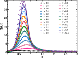
FIG. SM 1: Theoretical snapshots (solid lines) of the small-$k$ peak of $S(k;t)$ (for the same conditions indicated in Fig. 2 of our Letter), compared with the snapshots of a Brownian-dynamics simulated quench (symbols) and with waiting times adjusted to match the height $S(k_{max};t)$ of this peak.

In Fig. 2 of our Letter, the sequence of simulated snapshots of $S(k;t)$ was compared with the corresponding theoretical sequence, with identical evolution times $t$, thus exhibiting the quantitative inaccuracies of the approximate theory, most notably a quantitative mismatch between the simulation and the theoretical clocks. In spite of this difference, however, the structural pathways predicted by theory and registered by simulations are remarkably similar. This is illustrated here in Fig. SM1, which compare the same sequence of simulated snapshots of $S(k;t)$ in Fig. 2 of our Letter, but now paired with the theoretical snapshots having the same height $S_{max}(t)$ (but, obviously, different evolution time).

I.5 Arrested spinodal decomposition in protein solutions.

Here we provide the quantitative details of the comparisons in Figs. 3, 4(a)-(b) and 5(a)-(b) of the Letter, between our theoretical predictions and the reported experimental measurements of the growth and arrest of the spinodal heterogeneities of gelling protein solutions.

I.5.1 Gelling lysozyme solutions.

In Fig. 2(d) of Ref. gibaud , Gibaud and Schurtenberger report the experimental measurements of the growth and arrest of the representative size $\xi(t)$ (in micrometers) of the heterogeneities, as a function of time (in seconds), of gelling lysozyme proteins of diameter $\sigma=3.4nm$ in aqueous solution at fixed bulk concentration corresponding to a volume fraction of approximately $\phi=0.15$. To compare our predicted theoretical scenario with these data, let us normalize their experimental $\xi(t)$ and $t$ obtained by microscopy, by the experimental value of our theoretical units of length and time, $\sigma$ and $\tau_{B}\equiv\sigma^{2}/D_{0}$. Using Stokes-Einstein’s relation and the viscosity of water at room temperature we obtain $D_{0}=122\mu m^{2}/s$ and $\tau_{B}=\sigma^{2}/D_{0}=1\times 10^{-7}s$.

Plotted in this manner, the experimental data of Fig. 2(d) of Ref. gibaud appear as the empty symbols in Fig. SM 2. In this figure the solid lines are the theoretical predictions for the evolution of $\xi(t)$ in the HSAY model with $z=2$ initially at the (theoretical) temperature $T_{0}=1.5$ and quenched at fixed volume fraction ($\phi=0.15$) to various values of the final temperature $T$. The region limited by the dotted lines is the time-window employed in the inset of Fig. 2(b). As we can see, in reality the experimental data fall well outside such time-window. However, as our present comparison demonstrates, one can find a theoretical curve (red line) corresponding to a value of $T$ closer to the spinodal curve, whose predicted arrest also occurs far outside this window and approximately superimposes on the experimental data. The Fig. SM 2 also re-plots, now as solid symbols, the same experimental data with $\xi(t)$ and $t$ arbitrarily reduced by empirical factors (7 $\times 10^{-3}$ and 1.5 $\times 10^{-8}$, respectively). We do this only to illustrate, as we do in the inset of Fig. 2(b) of the Letter, their qualitative resemblance with the predicted scenario of the demonstrative quench of the HSAY model discussed in that figure (notwithstanding the fact that the theoretical curves there actually refer to the isochore $\phi=0.08$).

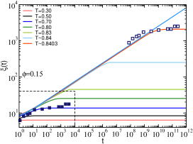
FIG. SM 2: Theoretical evolution (solid lines) of the size $\xi(t)$ of the heterogeneities of the HSAY model for a sequence of quenches for several final temperatures. The empty square symbols are the experimental results measured in a lysozyme protein system reported in Fig. 2(d) of Ref.gibaud . The solid symbols represent the scaled data.

Of course, comparing theoretical results for the HSAY model with experimental data for the referred protein solution can only have the purpose of comparing the essential qualitative features of the striking arrest of the process of spinodal decomposition. To establish a more proper quantitative comparison, the theoretical calculations should be fine-tuned to actually correspond to the detailed experimental conditions (much smaller range of the attractive potential ($z>>2$), finite cooling rates, etc.), which is for the moment out of the scope of this short communication.

I.5.2 Gelling bovine serum albumin solutions.

To complement the previous comparison, let us now refer to Fig. 7 of reference davela , where Da Vela et al. report quite similar experimental measurements of $\xi(t)$ for a sequence of quenches involving another protein, namely, bovine serum albumin, quenched along its critical isochore (protein concentration $175mg/mL$ BSA with 44 mM YCL₃). This protein has diameter $\sigma=6nm$, and in the reported solution presents a lower consolute temperature. Thus, in contrast with the previous example, a deeper quench involves a higher experimental temperature $T_{e}$. Nevertheless, to compare these measurements with our predicted scenario we followed essentially the same procedure described above, and the result is summarized in Fig. 3(a) of the Letter.

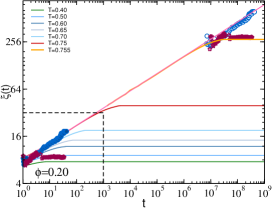
FIG. SM 3: Theoretical evolution (solid lines) of the size $\xi(t)$ of the heterogeneities of the HSAY model for a sequence of quenches for several final temperatures. The symbols are the experimental results measured in the BSA solutions reported in Fig. 7 of Ref. davela , for two of the systems (squares for $T=30^{o}C$ and circles for $T=57.5^{o}C$). The solid symbols represent the scaled data.

To explain this procedure in more detail, let us mention that in this case we estimated $D_{0}=60\mu m^{2}/s$ and $\tau_{B}=1\times 10^{-6}s$. In Fig. SM 3, we thus plot the normalized experimental data (empty symbols) corresponding to the shallowest and to the deepest quenches reported in Fig. 7 of reference davela (labeled there by the experimental temperatures $T_{e}=30^{o}C$ and $57.5^{o}C$, respectively). The solid lines are theoretical predictions for the evolution of $\xi(t)$ in the HSAY model with $z=2$ initially at the (theoretical) temperature $T_{0}=1.5$ for various values of the final temperature $T$. Since the experiments were conducted at the volume fraction $\phi=0.20$, the theoretical quenches were performed at the same volume fraction.

Once again, the experimental data fall well outside the time-window employed in the inset of Fig. 2b, but again, one can find theoretical curves corresponding to values of $T$ closer to the spinodal curve, whose predicted arrest approximately superimposes on these experimental data. This Fig. SM3 also re-plots (solid symbols) the same experimental data with $\xi(t)$ and $t$ arbitrarily reduced by empirical factors (3.1 $\times 10^{-2}$ and 1 $\times 10^{-7}$, respectively). This is exactly what we have done to generate Fig. 3(a), which also includes the experimental results for the other quenches reported in Fig. 7 of reference davela .

I.6 Arrested spinodal decomposition in colloid-polymer mixtures.

Let us now discuss the details of the comparisons in Figs. 3(b), 4(a)-(b) of the Letter, which refer to the experimental measurements of the evolution of $\xi(t)$ in two colloid-polymer mixtures that differ in the range of the depletion attraction between colloids.

I.6.1 Moderate polymer/colloid size ratio: longer-ranged depletions.

In Fig. 3(b) of the Letter we quote the experimental measurements by Zhang et al., reported in Fig. 5(a) of Ref. royall , of the growth and arrest of $\xi(t)$ in a colloid-polymer mixture where the mean diameter of the colloids is 544 nm and the polymer radius of gyration is 126 nm, so that the range $\delta$ of the depletion forces between colloids induced by the polymer (in units of the colloid’s diameter) is $\delta\approx 0.45$. This means that, regarding the range of the attractive interactions, this system is represented more closely (than the previous protein solutions) by the HSAY model with $z=2$, discussed and simulated in Fig. 2 of our Letter.

Ref. royall determines that for these experimental systems $\tau_{B}\approx 0.7s$ and reports the data already in units of $\sigma$ and $\tau_{B}$ for a system with fixed colloid volume fraction $\phi=0.20$ and for several values of the polymer concentration $C_{p}$, whose inverse plays the role of the theoretical temperature $T$. In Fig. 3(b) of the Letter we plot these experimental data along with our theoretical predictions for a sequence of quenches along the isochore $\phi=0.20$. Here again, to put both theory and experiments in the same time window, so as to appreciate the qualitative agreement, the experimental data of $\xi(t)$ and $t$ were arbitrarily multiplied by empirical factors (6 and 9, respectively), much more moderate than in the previous case involving protein solutions.

I.6.2 Small polymer/colloid size ratio: short-ranged depletions.

Figs. 4(a) and (b) of our Letter reproduce, respectively, the experimental data reported by Lu et al. in Figs. 4(b) and (c) of Ref. lu , corresponding to a colloid-polymer mixture with colloid radius 560 nm and colloid-to-polymer size ratio $z=\sigma/2R_{g}\approx 17$. In these experiments, the transition to arrested or gelled states is investigated as a function of the polymer concentration, which plays the role of an effective temperature. These experiments monitor the non-equilibrium evolution of the colloid-colloid static structure factor $S(k;t)$ and of its first moment $k_{1}(t)\equiv\int_{0}^{k_{c}}kS(k;t)dk/\int_{0}^{k_{c}}S(k;t)dk$ (where $k_{c}$ locates the minimum of $S(k;t)$ following its low-$k$ peak), after a quench from a polymer concentration $c_{p}=0$ to $c_{p}=53.31$ mg/ml, keeping the colloid volume fraction fixed at $\phi=0.045$. The viscosity of the solvent is reported to be $\eta=1.96\times 10^{-3}$Pa $\cdot$ s at the temperature $T=25^{o}$C. Using the Stokes-Einstein relation we obtain the short time self diffusion coefficient as $D_{0}=0.19\mu m^{2}/s$, yielding a characteristic time $\tau_{B}=\sigma^{2}/D_{0}=6.3s$, which is the time unit employed in Figs. 4(a) and (b) of our Letter. The measured wave-vector $k_{1}(t)$ decreases with time until reaching the stationary arrested value $k_{1}^{a}\approx 0.45$.

To establish the connection between theory and experiments, we first solved the NE-SCGLE Eqs. (3)-(8) to theoretically calculate the first moment $k_{1}(t)$ for a sequence of quenches along the isochore $\phi=0.045$ of the HSAY model ($z=2$), starting at the same (high) initial temperature and with varying (lower) final temperature $T$. We then determined the $T$-dependent limiting value $k_{1}^{a}=\lim_{t\to\infty}k_{1}(t)$, and chose as the effective temperature of the experimental quench, the value of $T$ for which the condition $k_{1}^{a}(T)\approx 0.45$ was satisfied, yielding $T\approx 0.5$. In Fig. 4(a) of the Letter we compare the solution of Eqs. (3)-(8) for $S(k;t)$ after this particular quench, with the corresponding experimental data. Fig. 4(b) of the Letter presents a similar comparison between the theoretical (thick solid line) and experimental (full circles) time-dependent first moment $k_{1}(t)$.

The direct comparison between theory and experiment presented in Fig. 4 of the Letter illustrates that, in spite of appreciable quantitative discrepancies, most notably the mismatch between the theoretical and experimental clocks, there is a remarkable qualitative similarity.

References

- (1) P. E. Ramírez-González and M. Medina-Noyola, Phys. Rev. E 82, 061503 (2010).
- (2) P. Mendoza-Méndez, E. Lázaro-Lázaro, L. E. Sánchez-Díaz, P. E. Ramírez-González, G. Pérez-Ángel, and M. Medina-Noyola, Phys. Rev. E 96, 022608 (2017).
- (3) P. E. Ramírez-González and M. Medina-Noyola, Phys. Rev. E 82, 061504 (2010).
- (4) R. Juárez-Maldonado, M. A. Chávez-Rojo, P. E. Ramírez-González, L. Yeomans-Reyna and M. Medina-Noyola , Phys. Rev. E 76, 062502 (2007).
- (5) L. E. Sánchez-Díaz, P. E. Ramírez-González, and M. Medina-Noyola, Phys. Rev. E 87, 052306 (2013).
- (6) J. M. Olais-Govea, L. López-Flores, and M. Medina-Noyola, J. Chem Phys. 143, 174505 (2015).
- (7) R. V. Sharma and K. C. Sharma, Physica A 89, 213 (1977).
- (8) J. K. Percus and G. J. Yevick, Phys. Rev. 110, 1 (1957).
- (9) L. Verlet and J.-J. Weis, Phys. Rev. A 5 939 (1972).
- (10) M. P. Allen and D. J. Tildesley, Computer Simulation of Liquids (Oxford University Press, Oxford, 1887).
- (11) J. F. M. Lodge and D. M. Heyes, J. Chem. Soc., Faraday Trans., 93, 437 (1997).
- (12) T. Gibaud and P. Schurtenberger, J. Phys.: Condens. Matter 21, 322201 (2009).
- (13) S. Da Vela et al., Soft Matter, 12, 9334 (2016).
- (14) Isla Zhang, C. Patrick Royall, Malcolm A. Faersd and Paul Bartlett, Soft Matter, 9, 2076, (2013).
- (15) P. J. Lu, E. Zaccarelli, F. Ciulla, A. B. Schofield, F. Sciortino and D. Weitz, Nature 453, 499 (2008).