arXiv:1807 LU-TP 18-20 MCNET-18-13 PISTA: Posterior Ion STAcking

Abstract

We present a program allowing for the construction of a heavy ion Monte Carlo event using a general purpose proton–proton event generator of the users’ choice to deliver sub–collisions. In this heavy ion event, one or more jets can be added, again using a jet calculation of the users’ choice, allowing for more realistic simulation studies of jets in a heavy ion background.

PROGRAM SUMMARY

Program Title: PISTA: Posterior Ion STAcking
Licensing provisions: GPLv3
Programming language: Python
Supplementary material:
Journal reference of previous version:
Does the new version supersede the previous version?:
Reasons for the new version:
Summary of revisions:*
Nature of problem: high–energy collisions of heavy nuclei with protons or each other, are used to study the influence of a Quark–Gluon Plasma on particle production mechanisms. The relation between calculations of such effects, and the complex underlying final state is poorly understood, making correct comparison between theory and data difficult.
Solution method: the underlying event is generated in a multi-step procedure, relying on a calculation of collision geometry, as well as input from a proton–proton Monte Carlo event generator, run by the user. This allows the user to pick and choose between different well-understood proton–proton models for the underlying event. Secondly, the signal process can be supplied either from a proton–proton generator, or from a generator implementing interactions with a Quark–Gluon Plasma.
Additional comments including Restrictions and Unusual features: The user must install the input event generator(s), which must be able to output events in the standard HepMC event format [1].

1 Introduction

Hadron collisions are complex processes involving many different phenomena from the soft and the electroweak sector, some calculable by perturbative techniques, and some – especially in the case of soft QCD processes – relies on the use of models. Over the past 20 years, such techniques have been refined and implemented into so-called General Purpose Monte Carlo Event Generators, such as Herwig 7 [1], Pythia 8 [2] and Sherpa [3], which provide a very good description of most aspects of hadronic collisions. The connection between these well-understood models of hadronic collisions, and collisions of heavy nuclei are, however, lacking.

Existing event generators for the study of jets in heavy ion collisions are roughly speaking divided into two categories. In the first category, there are generators which modify a proton–proton (pp) simulation according to a set of assumptions about the influence of a Quark-Gluon Plasma on the jet evolution. Generators such as JEWEL [4] and the JETSCAPE generators [5] place themselves in this category. On the other hand, generators such as HIJING [6] or the recent Angantyr addition to Pythia 8 [7, 8] aim to describe the full event. Generators of the latter type are generally better suited to investigate the influence of the heavy ion ”underlying event”, i.e. the presence of several jets from almost uncorrelated sub-collisions, disturbing the jet signal of interest. In spite of these generators’ ability to generate full events, a user is still faced with a problem given the task of (a) generating a jet using a given standard tool (with or without the assumption of a plasma) (b) embedding this into a realistic underlying event. Though a seemingly trivial task, it is nevertheless important to carry this task out with sufficient rigour; in particular, one cannot assume that an underlying event consists of a number of uncorrelated pp collisions, as one will at least have to respect energy–momentum conservation, restricting the phase space of the underlying event. It is also important for a more technical reason. When comparing heavy ion calculations to data, the comparison is usually carried out at various ”centralities”, understood as the impact parameter at which the nuclei have collided. Since the impact parameter is not experimentally accessible, experiments use a different definition, usually based on event activity. Therefore a direct comparison is at least difficult. With a full simulation of the underlying event, the direct comparison is enabled by construction.

The present program introduces a modified implementation of the underlying event model first introduced in the Fritiof event generator [9, 10], and recently implemented in Pythia 8 [7, 8], with the caveat that this implementation allows for a given HepMC [11] compatible pp event generator to produce the underlying event, and a given HepMC compatible generator to produce the signal event. This allows the user to perform a quantitative simulation study of jets in a semi-realistic heavy ion background.

2 Structure of the program

For the program to work, input from one or more event generator(s) supporting the HepMC event standard is needed. The event generator input is read from FIFO–pipes and an initial state calculation determines how many events should be taken from each pipe, and used to build up a full proton–Nucleus (pA) or Nucleus–Nucleus (AA) event. The program is written in Python, and structured in two programmatic parts.

1. An initial state calculation determining how many sub-collisions a given event should consist of.

2. A simulation step taking input from the event generators, and piping it, according to the initial state calculation, into a full pA or AA event.

The program workflow contains several logic parts, as indicated in the flowchart in figure 1. A Glauber calculation is performed, and serves, along with the event generator output, the input to the decision process, determining how many events and which types of events should be merged into a heavy ion event. The output is a HepMC event with an associated weight, which the user can perform an independent analysis of inside the Python framework itself or pipe to an external analysis framework such as Rivet [12]. We highly recommend the user to take advantage of the latter option.

Figure 1: Flowchart indicating the typical workflow. The user initializes a Glauber calculation along with the input generator(s), the events are merged together, and a single heavy ion event is produced in the HepMC format.

Before running the program, the user should download and compile the event generator(s) they desire to use. The program comes with sample run cards for Herwig 7, as well as sample programs for Pythia 8, ready to use with the default installation of the two event generators. The program itself is written in Python, and is highly customizable. In the main script, the user should set paths to event generator supplied FIFO–pipes, as well as basic run information related to the colliding nuclei.

3 Glauber calculation

To determine the number of sub-collisions needed to generate the full heavy ion collision, a so–called Glauber [13] calculation is performed. Nucleons are placed in a Woods-Saxon potential in a stochastic manner, nuclei from projectile and target which are overlapping in impact-parameter space, are counted as ”collided” in a given event.

The user must supply the Glauber calculation with the nuclear PDG number (on the form 100ZZZAAAI for nuclei, 2212 for protons) as well as the inelastic, non–diffractive cross section for a nucleon–nucleon collision ($\sigma_{NN}$) at the desired collision energy.

The Glauber calculation can in principle be run stand-alone, should a user desire to do that. In such cases, the calculation should be initialized in a similar way and information about the position of individual sub–collisions can be accessed by calling the next method of the initialized Glauber object. This returns a list of particles and sub–collision, which can be examined further.

3.1 Sampling the Woods-Saxon distribution

The nucleus’ transverse structure is described by a Woods-Saxon distribution. We use here the parametrization by Broniowski et al. known as the GLISSANDO parametrization [14, 15] with a density function:

$$\rho(r)=\frac{\rho_{0}(1+wr^{2}/R^{2})}{1+\exp((r-R)/a)}.$$ (1)

Here $R$ is the nuclear radius, $a$ is the nuclear skin width, $\rho_{0}$ is the central density (not used in the present calculation) and $w$ the Fermi parameter.

3.2 Performing sub-collisions

The nuclear impact parameter is chosen from a Gaussian distribution, and in the default mode, the two nuclei are collided using the simplest possible recipe, namely by treating each nucleon as a black disk with radius $\sqrt{\sigma_{NN}/4\pi}$. If two nuclei are overlapping, they collide. In figure 2 (left) a sample PbPb collision is shown. Grey nucleons do not participate, while the participant nucleons from target and projectile are coloured red and blue respectively. The geometry of an event is chosen such that the target sits at coordinates (0,0), while the projectile is shifted by the impact parameter as well as an event plane angle.

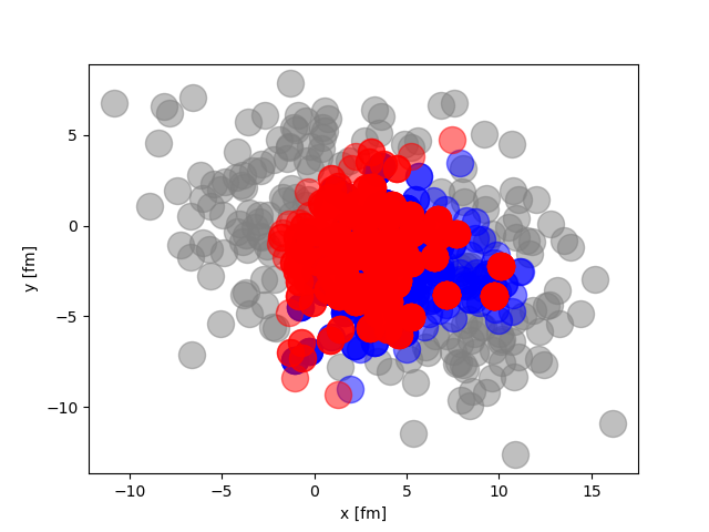
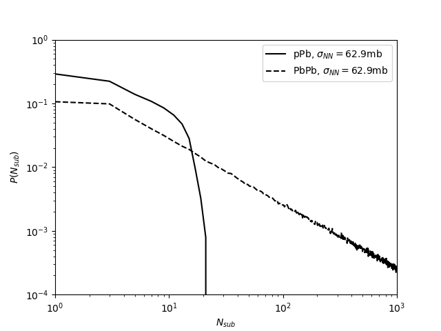
Figure 2: (left) Sample PbPb-event at intermediate impact parameter, showing overlapping nucleons leading to sub-collisions. (right) The distribution of number of sub-collisions in PbPb and pPb with $\sigma_{NN}=62.9$mb, indicating the vast difference in complexity for the two types of systems.

The physical value for $\sigma_{NN}$ is the only free parameter. The user can either insert a value as desired or rely on a calculated value. The program includes a simple implementation of the Schuler–Sjöstrand model [16] which, given the center–of–mass energy, outputs the total, elastic and single diffractive cross sections, calculated using a fairly standard Pomeron–based scheme. The user may prefer to use experimentally obtained values instead, and rely on the Schuler–Sjöstrand model only in cases where measurements are not available.

For the purpose of studying the background to jets in heavy ion collisions, such a simple treatment ought to be enough. The program is, however, devised in such a way that the user can easily extend to other, more sophisticated models for sub-collisions. The basic functionality is implemented in a class called GlauberBase, which for the case of black–disk–collisions, is derived from a class called BlackDisk, which is the class instantiated by the user. Should a user wish to collide for example semi-transparent disks, such a class can be added by the user, inheriting from the same base class. Thus all basic functionality is retained, and the user needs only implement the functionality connected to the semi-transparent disk.

In figure 2 (right), the distribution of number of sub–collisions for a sample pPb system and a sample PbPb system is shown. Note that the $x$-axis is logarithmic, indicating that the computational complexity for treating a PbPb system can be orders of magnitudes larger than a pPb system. The reason being that each projectile nucleon has the possibility to interact with several target nucleons, none being limited to only one interaction.

3.3 Glauber–Gribov fluctuations

In asymmetric pA collisions, it is of key importance to include colour fluctuations of the projectile, allowing $\sigma_{NN}$ to fluctuate event by event, to get a realistic estimate of the number of sub-collisions [17]. For this purpose a GlauberGribov model has been implemented as an extension to GlauberBase, where $\sigma_{NN}$ is drawn from a log–normal distribution [7]:

$$P(\ln(\sigma_{tot}))=\frac{1}{\Omega\sqrt{2\pi}}\exp\left(\frac{\ln^{2}(\sigma_{tot}/\sigma_{0})}{2\Omega^{2}}\right),\sigma_{NN}=\lambda\sigma_{tot}.$$ (2)

Parameters suitable for 5.02 TeV collisions, $\Omega=0.25,\sigma_{0}=85,\lambda=0.63$ are set by default.

4 Merging sub-events

The backbone of the Angantyr merging recipe is the notion of ”secondary absorptive” sub–collisions. The concept is most easily explained in the simple case of a proton–Deuteron (pD) collision. Consider the case where the proton has colour exchange with both Deuteron constituents. Clearly,at least one colour exchange must exist over the full kinematically allowed rapidity span of the event. Further exchanges do not have to but can span only a part of this. In pp event generators various so–called ”colour reconnection” models lead to such effects. In the pD collision, the same mechanism is mimicked by labelling one of the two sub–collisions as the ”primary” one, and the other as the ”secondary” one. The primary one will contribute to the final state as a normal pp collision (including colour reconnection), but the secondary one does not need to have even a single colour exchange over the full kinematically allowed region. It is observed [8] that such secondary absorptive events contributes approximately like a single diffractive event, and will thus be modelled as such.

For a full explanation of this procedure, and its generalization to AA collisions, we refer to ref. [8].

4.1 Combination of events

Even given the recipe presented for combining sub-events presented in Angantyr, one is left with several choices regarding specific implementation. In the current program the sub-events are combined as follows:

1. Sort possible collisions from Glauber calculations according to their impact parameter (most central first).

2. If none of the participants was used in a ”harder” (defined below) event, this sub-collision is labelled ”hard”.

3. If one of the participants was ’used’ before, its labelled as additional_side, with side being the direction the participant was used in a previous harder collision. The other participant is then also labelled as used and therefore removed from possible hard processes.

4. If both participants have been used before in harder collisions, we label the sub-collision as additional_both.

Here, the measure of hardness is calculated in the selectHardest function. The user can select between several hardness measures, or define their own. The default supplied (and recommended) defines hardness as the scalar sum of hadron $p_{\perp}$ (dubbed HT in the program). The implementation details of how to fill the list according to hardness are outlined in A. For example in a pA collision, this will produce one ’hard’ event and since the proton was then ’used’, the additional sub-collisions are added to the nucleus side. Once the labelling is performed, the main event is defined by the hardest sub-collision. In the spirit of ref.  [7] the main event and the following hard sub-collisions are chosen to be the hardest of a $N_{sub}$ of absorptive QCD events.

4.2 Momentum conservation

In order to include momentum conservation we employ a very primitive scheme to restrict the momentum in beam directions to not exceed the incoming energies. Since events produced by an arbitrary generator are used, the program should not rely on event record information. Instead we keep track of the sum of incoming momentum in $z$-direction for each participant and add for each stacked event the sum of final state particles in a given rapidity range $[0,\eta]$ and $[-\eta,0]$ to the corresponding incoming participant. If the next event exceeds the allowed incoming momentum we do not add the corresponding event.

The default cut-off value is set to $\eta=7.0$, which includes the acceptance of all present detector experiments, but excludes beam remnants. The user can change this value if desired.

4.3 Adding a signal process

It is possible to add a signal process in the sub–collision with smallest impact parameter, by generating the process using the input generator to create another FIFO–pipe containing those events. As indicated in the introduction, we foresee the most common use case of the program will be to add a signal event such as $Z+$jet(s) or di–jets with or without the assumption of a medium, and use the program to study the behaviour of the jet in a heavy ion background. If one wishes to have the correct cross section for such an event, the event should be reweighted with a factor $N_{sub}\sigma_{signal}/\sigma_{NN}$, where $N_{sub}$ is the number of sub-collisions.

Since different general purpose event generators have different models for QCD MPI events and different Matrix Element + Parton shower matching and merging schemes implemented, it might be beneficial to take the heavy ion background from one generator, and adding a signal from another generator. This can be done directly by setting up FIFO–pipes from the separate generators.

It is also possible to add a signal process from an event generator which includes a medium response, such as JEWEL or a JETSCAPE event generator. This will enable a study of the medium modified jet in a realistic background simulation.

4.4 Tuning

General purpose MC generators include several parameters for describing multi parton interactions, defining the underlying event to a signal process in pp. If these parameters are changed, the model, of course, loses its predictive power for minimum bias heavy ion observables, but if the purpose is to provide modelling of the background to a signal process, this predictive power can be traded off for a better description of the underlying event. In such cases, the user might want to retune these parameters. Users are referred to user manuals for input generators to carry out this process, we provide two sample Rivet analyses for pA, and one for AA, to do such a retuning. The sample results in the next section are all using default tunes.

5 Reading out results

Results are written out in HepMC format, enabling easy comparisons to data using the Rivet framework, or can be analysed directly by the user. In this section we demonstrate the program functionality by showing comparisons of minimum bias pPb and PbPb data to Pista + Pythia 8 and Pista + Herwig 7, but remind that any pp generator able to fulfil the requirements listed in section 4, and can produce HepMC output files can be substituted for those. Secondly, we demonstrate sample results obtained by embedding a $Z$+jet events into PbPb collisions. We demonstrate using first Pythia 8 and Herwig 7 signal events, following up with events produced using JEWEL [18]. But also here any generator able to produce HepMC events can be used.

The Rivet comparison routines used here are shipped with the program to allow the user to reproduce all plots shown in this paper directly.

5.1 Minimum bias results

We present here comparisons to multiplicity distributions obtained with the ATLAS and ALICE experiments at the LHC in the case of pPb [19] and PbPb [20, 21] collisions. This serves the purpose of demonstrating that for the case of minimum bias collisions, the model does well in estimating the total particle production. Thus the model provides a sensible baseline for modelling the underlying event to a jet.

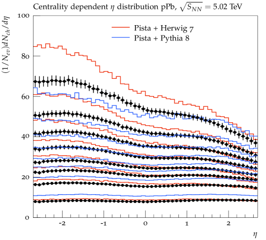
Figure 3: Centrality dependent $\eta$ distributions of charged primary particles in pPb collisions at $\sqrt{s_{NN}}=5.02$ TeV, obtained by ATLAS [19]. Centralities ranging from top to botton are: 0-1%, 1-5%,…,60-90%. Experimental results are compared to Pista + Pythia 8 and Pista + Herwig 7.

The centrality measure used for comparison is the same as (or similar to) the ones used in the experimental analyses. In the case of ATLAS analyses, the centrality measure is defined as the $\sum E_{\perp}$ of particles in $2.09<|\eta|<3.84$ (only the Pb going side for pPb), which can be directly applied. For ALICE analyses no direct, particle level observable exist, as the centrality observable is not detector unfolded. We use, as a proxy for the centrality observable, $\sum E_{\perp}$ of charged particles in the relevant detector acceptance. This, as well as the implementation of experimental cuts, can be changed as desired.

As mentioned in section 3.3, Glauber-Gribov fluctuations are necessary to reproduce the centrality observable in pPb collisions, and is thus employed for those results. We will not go further into the physics details of this point here, but it would be well worth to further study the effects of such fluctuations on final state observables.

In figure 3 we show multiplicity in pPb collisions as a function of pseudo-rapidity, in bins of centrality as defined above. While the Pista + Herwig 7 description (red line) visibly overshoots most of the distributions, the Pista + Pythia 8 (blue line) simulation undershoots the very central event multiplicity and overshoots more peripheral event multiplicities.

While the tilt in the multiplicity distributions in the Herwig 7 description is slightly too steep w.r.t. data, the Pythia 8 comparison shows an opposite less tilted behaviour w.r.t. data.

It is worth mentioning that a better agreement can be achieved by independent retuning the parameters used in the Pista implementation for the two generators. In this contribution, we limit ourselves to show distributions with equal parameters on the Pista part and default parameter settings on the generator side.

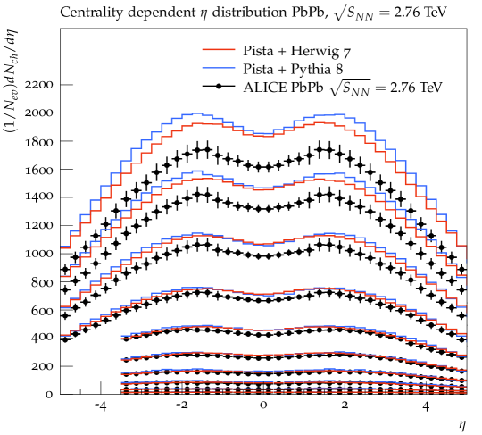
Figure 4: Centrality dependent $\eta$ distributions of charged primary particles in PbPb collisions at $\sqrt{s_{NN}}=2.76$ TeV, obtained by ALICE [20]. Centralities ranging from top to botton are: 0-5%, 5-10%,…,80-90%. Experimental results are compared to Pista + Pythia 8 and Pista + Herwig 7.

In figure 4 we show the multiplicity of charged particles in Pb-Pb collisions as a function of pseudo-rapidity in bins of centrality. Both the generators overshoot the data for very central events by approximately 20% and show a better agreement for lower more peripheral collisions. Compared to the pPb comparison we observe a less pronounced discrepancy between the two generators. Compared to other models for heavy ion collisions, the description in this simple model is slightly worse than in the evolved Angantyr model implemented in Pythia 8, but similar to the HIJING [6] and AMPT [22] models. (For comparison to the latter models, see ref. [20].) We do not carry out any detailed comparison to other models in this paper, as this is beyond the scope of a manual, but defer it to a coming publication.

In figures 5 and 6 we compare to $p_{\perp}$ distributions in PbPb collisions obtained by ATLAS [21]. The peripheral and semi-peripheral distributions in figure 5 are fairly described by both generators, Pista + Herwig 7 is systematically below Pista + Pythia 8, an investigation whether this is due to differences in the parton shower implementation or hadronization models in the generators would be interesting from a physics perspective.

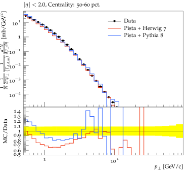
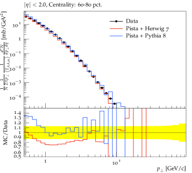
Figure 5: Centrality dependent $p_{\perp}$ distributions in PbPb collision at $\sqrt{s_{NN}}=2.76$ TeV, obtained by the ATLAS experiment [21]. Mid–central (50-60%) left and peripheral (60-80%) right.

The corresponding central distributions in figure 6 are described worse, similarly to the other previously mentioned event generators which does not include medium effects.

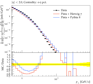
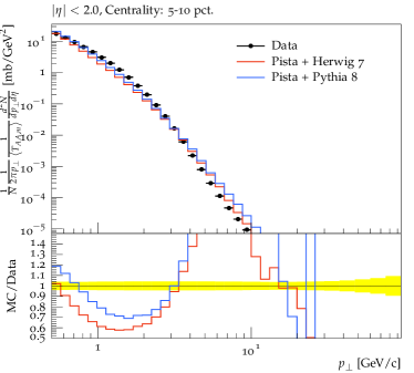
Figure 6: Centrality dependent $p_{\perp}$ distributions in PbPb collision at $\sqrt{s_{NN}}=2.76$ TeV, obtained by the ATLAS experiment [21]. Most central (0-5%) left and 5-10% right.

5.2 Results with an embedded jet

We now go on to demonstrate the addition of signal processes in the case of $Z$+jet events embedded in a PbPb background.

We provide not a full physics analysis but defer the discussion of such to a coming paper. We instead demonstrate the features by showing simple features of events with a $Z\rightarrow\mu^{+}\mu^{-}$ plus a jet reconstructed by the anti-kT algorithm implemented in FastJet [23]. A jet is said to be back-to-back with the $Z$ (reconstructed from the muon pair) if it has $\Delta\phi>7\pi/8$ with the reconstructed $Z$. The $Z$ is required to have $p_{\perp}>60$ GeV, and the muons $p_{\perp}>$10 GeV.

In figure 7 we show the jet-$p_{\perp}$ of the leading jet in the event for an embedded event, compared to the embedded pp event only, for a jet cone radius of $\Delta R=0.3,0.5$ and $0.7$. For comparison, we show Pista + Pythia 8 (left) and Pista + Herwig 7 (right). It is is directly visible that the chosen $\Delta R$ parameter has significantly higher influence in a PbPb embedded event than in a pp event, which should not be surprising as a PbPb event has much more underlying event activity, swept up by the jet algorithm. We note also that choosing a sufficiently narrow jet cone in PbPb makes the jet coincide with the pp jet. The Pista + Pythia 8 and Pista + Herwig 7 figures are very similar, as one would expect.

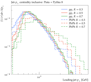
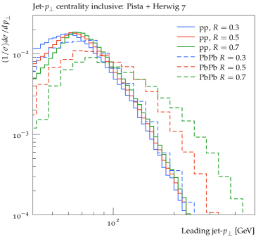
Figure 7: Transverse momentum of the leading jet for a $Z+$ jet event embedded into a PbPb event, using Pythia 8 (left) and Herwig 7 (right) respectively. In the figures jet cone radii of $\Delta R=0.3,0.5$ and $0.7$ are shown, and also compared to pp (i.e. the embedded signal only).

In figure 8 we show the centrality binned leading jet-$p_{\perp}$ for Pista + Pythia 8(left) and Pista + Herwig 7 (right). We note that the centrality definition in this figure is similar to what is done in an experiment, i.e. by binning in the same centrality observable as used in section 5.1. This is a natural feature of the embedding procedure, as the $Z+jet$ event is embedded in a full underlying event, but to the authors’ knowledge not possible in any state-of-the-art jet quenching simulation.

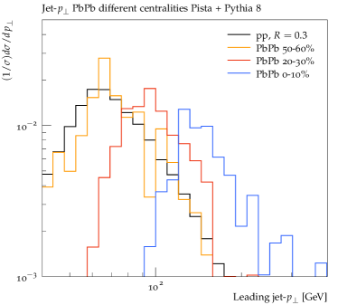
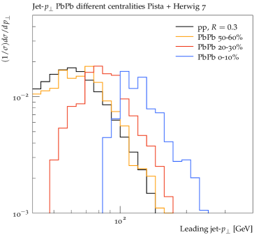
Figure 8: Centrality binned leading jet-$p_{\perp}$ embedded in a PbPb background for Pista + Pythia 8 (left) and Herwig 7 (right) respectively.

The centrality binned jet-$p_{\perp}$, has the striking feature that the spectrum is shifted upwards with increasing centrality. This is again not a surprising feature, as the increased underlying event activity will naturally manifest as ”misidentified” leading jets. This is, however, an effect which must be handled by experiments, and this demonstrates that this approach can be used directly to estimate the efficiency of subtraction techniques as employed by experiments (in eg. ref. [24]).

5.3 Embedding with JEWEL

Finally we demonstrate the ability to embed a signal event from a special purpose generator, with an underlying event from general purpose generators. For this purpose we use the JEWEL event generator [4, 18], which includes modifications to the jet from a Quark–Gluon Plasma.

The first thing to note is the centrality definition. In JEWEL, forward event activity in heavy ion collisions is not reproduced, and for the purpose of the medium calculation, a centrality (in percent) must be set. When embedded into a generated underlying event, the underlying event has a centrality based on event activity. These two centralities does not coincide. For the purpose of demonstration, we therefore select a JEWEL centrality between 0-10%, and show only events where this coincides with the underlying event centrality. For the purpose of a real physics analysis, the user ought to select a finer centrality binning.

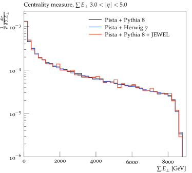
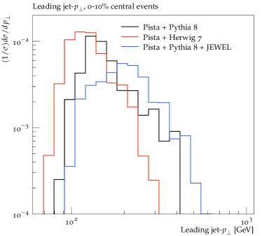
Figure 9: The centrality observable (left) used for PbPb collisions for Pista + Pythia 8, Herwig and (Pythia 8 + JEWEL) respectively. Transverse momentum (right) of the leading jet for 0-10% central events using Pista + Pythia 8, Herwig and (Pythia 8 + JEWEL) respectively.

In figure 9 (left), we show the PbPb centrality measure (as used in the previous sections) for Pista + Pythia 8 and Herwig 7 respectively, as well as for JEWEL events embedded with Pista + Pythia 8. The generated centrality measures are seen to coincide up to statistical errors. It is thus possible to select central JEWEL events with underlying event activity matching the input centrality. This is done in figure 9 (right), where $p_{\perp}$ of the leading jet, in the same $Z+$ jet setup as in the previous section, is shown. The JEWEL calculation is compared to the corresponding embedded vacuum calculations using Pythia 8 and Herwig 7.

6 Conclusions

We have presented a generator independent framework for stacking pp collisions to obtain pA and AA collisions, based on Angantyr. Full, hadronized events are stacked, using the HepMC event record, allowing this framework to be very useful for studies of jet quenching effects, as one can merge a quenched jet–event with an underlying event generated with standard pp tools. While this is the first time the simulation of HI simulations containing Herwig 7 events are directly compared to Pythia 8, we plan to follow up the publication of the framework with physics studies of standard jet–quenching observables embedded in such an underlying event.

The framework is fully implemented in Python, and relies only on desired input event generators. For convenience, we ship the framework with a set of already implemented Rivet analyses, useful for comparison to data.

Appendix A Correlated Collisions

In collisions with more than one nucleus on one of the beam sides it is possible that one of the participating nuclei is part in more than one sub-collisions. A sub-collisions is in this section treated as an index pair labelling the participants of the colliding particles. We assume that we constructed an algorithm that allows us to identify a sub-collision as hard or additional and construct corresponding index pair vectors $\mathcal{H}$ and $\mathcal{A}$. Each index can at most appear once in $\mathcal{H}$ but multiple times in $\mathcal{A}$. For a given index-pair $(i,j)$ in the $\mathcal{H}$ we construct a method to tell the number $N$ of events to choose the hardest.

1. If $\mathcal{A}$ is empty or does not contain $i$ in the left indices or $j$ in the right indices we choose from N=1.

2. Project $\mathcal{A}$ to a subset $\mathcal{A}_{(i||j)}$ where either $i$ is the left or $j$ is the right index. Model1: choose from the length of $\mathcal{A}_{(i||j)}$ as, $N=len(\mathcal{A}_{(i||j)})+1$

3. For each pair $(k,l)$ in $\mathcal{A}_{(i||j)}$ add one to $N$ if the index ($k$ if $l==j$ else $l$) does not appear in the corresponding side of $\mathcal{H}$ and $1/2$ if it does. Model2: Choose from resulting $N+1$.

The resulting two models are very simple and also the appearance of the same indices in the additional events needs to be studied but the purpose of this paper is to set the infrastructure and define the framework.

References

- [1] M. Dobbs, J. B. Hansen, The HepMC C++ Monte Carlo event record for High Energy Physics, Comput. Phys. Commun. 134 (2001) 41–46.

References

- [1] J. Bellm, et al., Herwig 7.0/Herwig++ 3.0 release note, Eur. Phys. J. C76 (4) (2016) 196. arXiv:1512.01178, doi:10.1140/epjc/s10052-016-4018-8.
- [2] T. Sjöstrand, S. Ask, J. R. Christiansen, R. Corke, N. Desai, P. Ilten, S. Mrenna, S. Prestel, C. O. Rasmussen, P. Z. Skands, An Introduction to PYTHIA 8.2, Comput. Phys. Commun. 191 (2015) 159–177. arXiv:1410.3012, doi:10.1016/j.cpc.2015.01.024.
- [3] T. Gleisberg, S. Höche, F. Krauss, M. Schönherr, S. Schumann, F. Siegert, J. Winter, Event generation with SHERPA 1.1, JHEP 02 (2009) 007. arXiv:0811.4622, doi:10.1088/1126-6708/2009/02/007.
- [4] K. C. Zapp, JEWEL 2.0.0: directions for use, Eur. Phys. J. C74 (2) (2014) 2762. arXiv:1311.0048, doi:10.1140/epjc/s10052-014-2762-1.
- [5] S. Cao, et al., Multistage Monte-Carlo simulation of jet modification in a static medium, Phys. Rev. C96 (2) (2017) 024909. arXiv:1705.00050, doi:10.1103/PhysRevC.96.024909.
- [6] X.-N. Wang, M. Gyulassy, HIJING: A Monte Carlo model for multiple jet production in p p, p A and A A collisions, Phys. Rev. D44 (1991) 3501–3516. doi:10.1103/PhysRevD.44.3501.
- [7] C. Bierlich, G. Gustafson, L. Lönnblad, Diffractive and non-diffractive wounded nucleons and final states in pA collisions, JHEP 10 (2016) 139. arXiv:1607.04434, doi:10.1007/JHEP10(2016)139.
- [8] C. Bierlich, G. Gustafson, L. Lönnblad, H. Shah, The Angantyr model for Heavy-Ion Collisions in PYTHIA8arXiv:1806.10820.
- [9] B. Nilsson-Almqvist, E. Stenlund, Interactions Between Hadrons and Nuclei: The Lund Monte Carlo, Fritiof Version 1.6, Comput. Phys. Commun. 43 (1987) 387. doi:10.1016/0010-4655(87)90056-7.
- [10] H. Pi, An Event generator for interactions between hadrons and nuclei: FRITIOF version 7.0, Comput. Phys. Commun. 71 (1992) 173–192. doi:10.1016/0010-4655(92)90082-A.
- [11] M. Dobbs, J. B. Hansen, The HepMC C++ Monte Carlo event record for High Energy Physics, Comput. Phys. Commun. 134 (2001) 41–46. doi:10.1016/S0010-4655(00)00189-2.
- [12] A. Buckley, J. Butterworth, L. Lönnblad, D. Grellscheid, H. Hoeth, J. Monk, H. Schulz, F. Siegert, Rivet user manual, Comput. Phys. Commun. 184 (2013) 2803–2819. arXiv:1003.0694, doi:10.1016/j.cpc.2013.05.021.
- [13] R. J. Glauber, Cross-sections in deuterium at high-energies, Phys. Rev. 100 (1955) 242–248. doi:10.1103/PhysRev.100.242.
- [14] W. Broniowski, M. Rybczynski, P. Bozek, GLISSANDO: Glauber initial-state simulation and more.., Comput. Phys. Commun. 180 (2009) 69–83. arXiv:0710.5731, doi:10.1016/j.cpc.2008.07.016.
- [15] M. Rybczynski, G. Stefanek, W. Broniowski, P. Bozek, GLISSANDO 2 : GLauber Initial-State Simulation AND mOre…, ver. 2, Comput. Phys. Commun. 185 (2014) 1759–1772. arXiv:1310.5475, doi:10.1016/j.cpc.2014.02.016.
- [16] G. A. Schuler, T. Sjöstrand, Hadronic diffractive cross-sections and the rise of the total cross-section, Phys. Rev. D49 (1994) 2257–2267. doi:10.1103/PhysRevD.49.2257.
- [17] M. Alvioli, M. Strikman, Color fluctuation effects in proton-nucleus collisions, Phys. Lett. B722 (2013) 347–354. arXiv:1301.0728, doi:10.1016/j.physletb.2013.04.042.
- [18] R. Kunnawalkam Elayavalli, K. C. Zapp, Simulating V+jet processes in heavy ion collisions with JEWEL, Eur. Phys. J. C76 (12) (2016) 695. arXiv:1608.03099, doi:10.1140/epjc/s10052-016-4534-6.
- [19] G. Aad, et al., Measurement of the centrality dependence of the charged-particle pseudorapidity distribution in proton–lead collisions at TeV with the ATLAS detector, Eur. Phys. J. C76 (4) (2016) 199. arXiv:1508.00848, doi:10.1140/epjc/s10052-016-4002-3.
- [20] K. Aamodt, et al., Centrality dependence of the charged-particle multiplicity density at mid-rapidity in Pb-Pb collisions at TeV, Phys. Rev. Lett. 106 (2011) 032301. arXiv:1012.1657, doi:10.1103/PhysRevLett.106.032301.
- [21] G. Aad, et al., Measurement of charged-particle spectra in Pb+Pb collisions at TeV with the ATLAS detector at the LHC, JHEP 09 (2015) 050. arXiv:1504.04337, doi:10.1007/JHEP09(2015)050.
- [22] Z.-W. Lin, C. M. Ko, B.-A. Li, B. Zhang, S. Pal, A Multi-phase transport model for relativistic heavy ion collisions, Phys. Rev. C72 (2005) 064901. arXiv:nucl-th/0411110, doi:10.1103/PhysRevC.72.064901.
- [23] M. Cacciari, G. P. Salam, G. Soyez, FastJet User Manual, Eur. Phys. J. C72 (2012) 1896. arXiv:1111.6097, doi:10.1140/epjc/s10052-012-1896-2.
- [24] A. M. Sirunyan, et al., Study of Jet Quenching with jet Correlations in Pb-Pb and Collisions at TeV, Phys. Rev. Lett. 119 (8) (2017) 082301. arXiv:1702.01060, doi:10.1103/PhysRevLett.119.082301.
- [25] A. Buckley, PyHepMC v0.5.0 http://doi.org/10.5281/zenodo.1304131.
- [26] L. Heinrich, hepmcanalysis v0.0.1 http://doi.org/10.5281/zenodo.1304131.