Approximate Survey Propagation for Statistical Inference

Abstract

Approximate message passing algorithm enjoyed considerable attention in the last decade. In this paper we introduce a variant of the AMP algorithm that takes into account glassy nature of the system under consideration. We coin this algorithm as the approximate survey propagation (ASP) and derive it for a class of low-rank matrix estimation problems. We derive the state evolution for the ASP algorithm and prove that it reproduces the one-step replica symmetry breaking (1RSB) fixed-point equations, well-known in physics of disordered systems. Our derivation thus gives a concrete algorithmic meaning to the 1RSB equations that is of independent interest. We characterize the performance of ASP in terms of convergence and mean-squared error as a function of the free Parisi parameter $s$. We conclude that when there is a model mismatch between the true generative model and the inference model, the performance of AMP rapidly degrades both in terms of MSE and of convergence, while ASP converges in a larger regime and can reach lower errors. Among other results, our analysis leads us to a striking hypothesis that whenever $s$ (or other parameters) can be set in such a way that the Nishimori condition $M=Q>0$ is restored, then the corresponding algorithm is able to reach mean-squared error as low as the Bayes-optimal error obtained when the model and its parameters are known and exactly matched in the inference procedure.

I Introduction

I.1 General Motivation

Many problems in data analysis and other data-related science can be formulated as optimization or inference in high-dimensional and non-convex landscapes. General classes of algorithms that are able to deal with some of these problems include Monte Carlo and Gibbs-based sampling neal2000markov , variational mean field methods wainwright2008graphical , stochastic gradient descent bottou2010large and their variants. Approximate message passing (AMP) algorithms ThoulessAnderson77 ; DonohoMaleki09 is another such class that has one very remarkable advantage over all the before mentioned: for a large class of models where instances are generated from a probabilistic model, the performance of AMP on large such instances can be tracked via a so-called state evolution bolthausen2014iterative ; bayati2011dynamics ; javanmard2013state . This development has very close connections to statistical physics of disordered systems because the state evolution that describes AMP coincides with fixed-point equations that arise from the replica and cavity methods as known in the theory of glasses and spin glasses MPV87 .

AMP and its state evolution have been so far mainly used in two contexts. On the one hand, for optimization in cases where the associated landscape is convex. This the the case e.g. in the original work of Donoho, Maleki, Montanari DonohoMaleki09 where $\ell_{1}$-norm minimization for sparse linear regression is analyzed, or in the study of the so-called M-estimators donoho2016high ; advani2016statistical . On the other hand, in the setting of Bayes-optimal inference where the model that generated the data is assumed to be known perfectly, see e.g. zdeborova2015statistical ; LesKrzZde17 , where the so-called Nishimori conditions ensure that the associated posterior probability measure is of so-called replica symmetric kind in the context of spin glasses MPV87 ; NishimoriBook . Many (if not most) of inference and optimization problems that are solved in the currently most challenging applications are highly non-convex and the underlying model that generated the data is not known. It is hence an important general research direction to understand the behavior of algorithms and find their more robust generalizations encompassing such settings.

In the present paper we make a step in this general direction for the class of AMP algorithms. We analyze in detail the phase diagram and phases of convergence of the AMP algorithm on a prototypical example of a problem that is non-convex and not in the Bayes-optimal setting. The example we choose is rank-one matrix estimation problem that has the same phase diagram as the Sherrington-Kirkpatrick (SK) model with ferromagnetic bias SherringtonKirkpatrick75 . AMP reproduces the corresponding replica symmetric phase diagram with region of non-convergence being given by the instability towards replica symmetry breaking (RSB). We note that while this phase diagram is well known in the literature on spin glasses, its algorithmic consequences are obscured in the early literature by the fact that unless the AMP algorithm is iterated with the correct time-indices bolthausen2014iterative convergence is not reached, see discussion e.g. in zdeborova2015statistical .

Our main contribution is the development of a new type of approximate message passing algorithm that takes into account breaking of the replica symmetry and reduces to AMP for a special choice of parameters. We call this the approximate survey propagation (ASP) algorithm, following up on the influential work on survey propagation in sparse random constraint satisfaction problems MPZ02 ; BMZ05 . We show that there are regions (away from the Nishimori line) in which ASP converges while AMP does not, and where at the same time ASP provides lower estimation error than AMP. We show that the state evolution of ASP leads to the one-step-replica symmetry breaking (1RSB) fixed-point equations well known from the study of spin glasses. This is the first algorithm that provably converges towards fixed-points of the 1RSB equations. Again we stress that, while the 1RSB phase diagram and corresponding physics of the ferromagnetically biased SK model is well-known, its algorithmic confirmation is new to our knowledge: even if the 1RSB versions of the Thouless-Anderson-Palmer (TAP) ThoulessAnderson77 equations was previously discussed, e.g. in MPV87 ; yasuda2012replica , the corresponding time-indices in ASP are crucial in order to reproduce this phase diagram algorithmically. Our work gives a concrete algorithmic meaning to the 1RSB fixed-point equations, and can thus be potentially used to understand this concept independently of the heuristic replica or cavity methods.

I.2 The low-rank estimation model and Bayesian setting

As this is a kind of exploratory paper we focus on the problem of rank-one matrix estimation. This problem is (among) the simplest where the ASP algorithm can be tested. In particular, for binary (Ising) variables it is equivalent to the Sherrington-Kirkpatrick model with ferromagnetically biased couplings as studied e.g. in SherringtonKirkpatrick75 ; de1978stability ; NishimoriBook . Low-rank matrix estimation is a problem ubiquitous in modern data processing. Commonly it is stated in the following way: Given an observed matrix $Y$ one aims to write it as $Y_{ij}=\lambda u^{\top}_{i}v_{j}+\xi_{ij}$, where $u_{i},v_{j}\in{\mathbb{R}}^{r}$ with $r$ being the rank, and $\xi_{ij}$ is a noise or a part of the data matrix $Y$ that is not well explained via this decomposition. Commonly used methods such as principal component analysis or clustering can be formulated as low-rank matrix estimation. Applications of these methods range from medicine over to signal processing or marketing. From an algorithmic point of view and under various constraints on the factors $u_{i},v_{j}$ and the noise $\xi_{ij}$ the problem is highly non-trivial (non-convex and NP-hard in worst case). Development of algorithms for low-rank matrix estimation and their theoretical properties is an object of numerous studies in statistics, machine learning, signal processing, applied mathematics, etc. wright2009robust ; candes2011robust ; candes2009exact . In this paper we focus on the symmetric low-rank matrix estimation where the matrix $Y_{ij}$ is symmetric, i.e. $Y_{ij}=Y_{ji}$ and the desired decomposition is $Y_{ij}=\lambda x^{\top}_{i}x_{j}+\xi_{ij}$, where $x_{i}\in{\mathbb{R}}^{r}$.

A model for low-rank matrix estimation that can be solved exactly in the large size limit using the techniques studied in this paper is the so-called general-output low-rank matrix estimation model lesieur2015mmse ; LesKrzZde17 where the matrix $Y_{ij}\in{\mathbb{R}}^{N\times N}$ is generated from a given probability distribution $P_{\rm out}^{(0)}(Y_{ij}|w_{ij}^{(0)})$ with

$$w_{ij}^{(0)}\equiv\frac{\left(x_{i}^{(0)}\right)^{T}x^{(0)}_{j}}{\sqrt{N}}\,,$$ (1)

and where each component $x_{i}^{(0)}\in{\mathbb{R}}^{r_{0}}$ is generated independently from a probability distribution $P_{0}(x_{i}^{(0)})$. The $N\times r$ matrix $X^{(0)}$ can then be seen as an unknown signal that is to be reconstructed from the observation of the matrix $Y_{ij}$.

Following Bayesian approach, a way to infer $X^{(0)}$ given $Y$ is to analyze the posterior probability distribution

$$P(X|Y)=\frac{1}{Z_{X}(Y)}\prod_{1\leq i\leq N}P_{X}(x_{i})\;\prod_{1\leq i<j\leq N}\exp\left[g\left(Y_{ij}|\frac{x^{\top}_{i}x_{j}}{\sqrt{N}}\right)\right]\,,$$ (2)

where $P_{X}(x_{i})$ is the assumed prior on signal components $x_{i}\in{\mathbb{R}}^{r}$ and $P_{\rm out}\left(Y_{ij}|w_{ij}\right)=\exp\left[g\left(Y_{ij}|w_{ij}\right)\right]$ is the assumed model for the noise. The normalization $Z_{X}(Y)$ is the partition function in the statistical physics notation. And the posterior distribution (2) is nothing else but the Boltzmann measure on the $r$-dimensional spin variables $x_{i}$.

In a Bayes-optimal estimation, we know exactly the model that generated the data, i.e.

$$P_{x}=P_{0},\quad P_{\rm out}=P_{\rm out}^{(0)},\quad r=r_{0}\,.$$ (3)

The Bayes-optimal estimator is defined as the one that among all the estimators minimizes the mean-squared error to the ground truth signal $x_{i}^{(0)}$. This is computed as the mean of the posterior marginals or, in physics language, the local magnetizations.

In this paper we will focus on inference with the mismatching model where at least one of the above equalities (3) does not hold. Yet, we will still aim to evaluate the estimator that computes the mean of the posterior marginals

$$\hat{x}_{i}=\int x_{i}P(X|Y)\prod_{j=1}^{N}{\rm d}x_{j}\,.$$ (4)

We will call this the marginalization estimator.

Another common estimator in inference is the maximum posterior probability (MAP) estimator where

$$\hat{X}^{\text{MAP}}=\underset{X}{\text{argmax}}\;P(X|Y)\,.$$ (5)

Generically, optimizing a complicated cost function is simpler than marginalizing over it, because optimization is in general simpler than counting. Thus MAP is often thought of as a simpler estimator to evaluate. Moreover, in statistics the problems are usually set in a regime where the MAP and the marginalization estimator coincide. However, this is not the case in the setting considered in the present paper and we will comment on the difference in the subsequent sections.

In our analysis we are interested in the high-dimensional statistics limit, $N\rightarrow\infty$ whereas $r=\mathcal{O}(1)$. The factor $1/\sqrt{N}$ in Eq. (1) in this limit ensures that the estimation error we are able to obtain is in a regime where it goes from zero to randomly bad as the parameters vary. This case is different from traditional statistics, where one is typically concerned with estimation error going to zero as $N$ grows.

In the $N\rightarrow\infty$ limit, the above defined model benefits of an universality property in the noise channel lesieur2015mmse ; LesKrzZde17 (see krzakala2016mutual for a rigorous proof) as the estimation error depends on the function $g$ only through the matrices

$$S_{ij}=\left.\frac{\partial g(Y_{ij}|w)}{\partial w}\right|_{w=0}\,, \hat{R}_{ij}=-\left.\frac{\partial^{2}g(Y_{ij}|w)}{\partial w^{2}}\right|_{w=0}\,.$$ (6)

Because of this universality, in the following we will restrict the assumed output channel to be Gaussian with

$$g\left(Y|w\right)=-\frac{(Y-w)^{2}}{2\Delta}-\frac{1}{2}\log 2\pi\Delta\,, S_{ij}=\frac{Y_{ij}}{\Delta}\,, \hat{R}_{ij}=\frac{1}{\Delta}\,.$$ (7)

The ground truth channel $P_{\rm out}^{(0)}(Y_{ij}|w_{ij}^{(0)})$ that was used to generate the observation $Y_{ij}$ is also Gaussian centered around $w_{ij}^{(0)}=x_{i}^{(0)}x_{j}^{(0)}/\sqrt{N}$ with variance $\Delta_{0}$.

I.3 Ferromagnetically biased SK model and related work

The numerical and example section of this paper will focus on one of the simplest cases of of rank-one $r_{0}=r=1$ estimation with binary signal, i.e.

$$P_{0}(x_{i})=P_{X}(x_{i})=\frac{1}{2}[\delta(x_{i}-1)+\delta(x_{i}+1)]\,.$$ (8)

In physics language such a prior corresponds to the Ising spins and the Boltzmann measure (2) is then the one of a Sherrington-Kirkpatrick (SK) model SherringtonKirkpatrick75 with interaction matrix $Y_{ij}$. After a gauge transformation $x_{i}\rightarrow s_{i}x_{i}^{(0)}$, $\xi_{ij}\rightarrow\tilde{\xi}_{ij}x_{i}^{(0)}x_{j}^{(0)}$ this is equivalent to the SK model at temperature $\Delta$ with random iid interactions of mean $1/N$ and variance $\Delta_{0}/N$ (see for instance the discussion in Sec. II.B of zdeborova2015statistical or Sec. II.F of zdeborova2010generalization ).

This variant of the SK model with ferromagnetically biased interactions is very well known in the statistical physics literature. The original paper SherringtonKirkpatrick75 presents the replica symmetric phase diagram of this model, de1978stability computes the AT line below which the replica symmetry is broken and Parisi famously presents the exact solution of this model below the AT line in parisi1979infinite . A rather complete account for the physical properties of this model is reviewed in MPV87 .

Note that while the replica solution and phase diagram of this model is very well known in the physics literature, the algorithmic interpretation of the phase diagram in terms of the AMP algorithm is recent. It is due to Bolthausen bolthausen2014iterative who noticed that in order for the TAP equations ThoulessAnderson77 to converge and to reproduce the features of the well known phase diagram, one needs to adjust the iteration indices in the TAP equations. We will call the TAP equations with adjusted time indices the AMP algorithm. Bolthausen proved that in the Sherrington-Kirkpatrick model the AMP algorithm converges if and only if above the de Almeida-Thouless (AT) line de1978stability .

The work of Bolthausen together with the development of AMP for sparse linear estimation and compressed sensing DonohoMaleki09 revived the interest in the algorithmic aspects of dense spin glasses. For a review of the recent progress see e.g. zdeborova2015statistical . AMP for low-rank matrix estimation was studied e.g. in rangan2012iterative ; NIPS2013_5074 ; DeshpandeM14 ; lesieur2015phase ; deshpande2015asymptotic ; lesieur2015mmse , its rigorous asymptotic analysis called the state evolution in bayati2011dynamics ; rangan2012iterative ; deshpande2015asymptotic ; javanmard2013state .

Correctness of the replica theory in the Bayes-optimal setting was proven rigorously in a sequence of work DeshpandeM14 ; deshpande2015asymptotic ; krzakala2016mutual ; barbier2016mutual ; LelargeMiolane16 ; barbier2017stochastic ; alaoui2018estimation . While the first complete proof is due to krzakala2016mutual , the Ising case discussed here is equivalent the Gauge-Symmetric Sherrington-Kirkpatrick proven earlier in korada2009exact . Various applications and phase diagrams for the problem are discussed in detail in e.g. LesKrzZde17 .

While it is well known in the physics literature de1978stability ; parisi1979infinite ; MPV87 that below the AT line replica symmetry breaking is needed to describe correctly the Boltzmann measure (2) the algorithmic consequences of that stay unexplored up to date. There are several versions of the TAP equations embodying a replica symmetry breaking structure in the literature MPV87 ; yasuda2012replica but they do not include the proper time-indices and hence will not be able to reproduce quantitatively the RSB phase diagram (just as it was the case for the TAP equations before the work of DonohoMaleki09 ; bolthausen2014iterative ).

In this paper we close this gap and derive approximate survey propagation, an AMP-type of algorithm that takes into account replica symmetry breaking. Using the state evolution theory rangan2012iterative ; DeshpandeM14 ; deshpande2015asymptotic we prove that the ASP algorithm reproduces the 1RSB phase diagram in the limit of large system sizes. We study properties of the ASP algorithm, resulting estimation error as a function of the Parisi parameter, its convergence and finite size behavior.

II Properties of approximate message passing

II.1 Reminder of AMP and its state evolution

In this section we recall the standard Approximate Message Passing (AMP) algorithm. Within the context of low-rank matrix estimation, the AMP equations are referred as Low-RAMP and are discussed extensively in LesKrzZde17 . In the physics literature, the Low-RAMP would be equivalent to the TAP equations ThoulessAnderson77 (with corrected iteration indices) for a model of vectorial spins with local magnetic fields and general kind of two-body interactions. In this sense, the Low-RAMP equations encompass as a special case the original TAP equations for the Sherrington-Kirkpatrick model SherringtonKirkpatrick75 , for the Hopfield model Mezard17 ; MPV87 and for the restricted Boltzmann machine GabTraKrz15 ; Traelal16 ; Mezard17 ; TubMon17 .

II.1.1 Low-RAMP equations.

Let us state the Low-RAMP equations to emphasize the differences and similarities with the replica symmetry breaking approach of Sec. III. The Low-RAMP algorithm evaluates the marginals of Eq. (2) starting from the belief propagation (BP) equations yedidia2003understanding (cf. the factor graph of Fig. 5 in the case where $s=1$). The main assumptions of BP is that the incoming messages are probabilistically independent when conditioned on the value of the root. In the present case the factor $1/\sqrt{N}$ in Eq. (1) makes the interactions sufficiently weak so that the assumption of independence of incoming messages is plausible at the leading order in the large size limit. Moreover, this assumption is particularly beneficial in the case of continuous variables: since we have an accumulation of many independent messages, the central limit theorem assures that it is sufficient to consider only means and variances to represent the result (relaxed-belief propagation) instead of dealing with whole probability distributions. To finally obtain the Low-RAMP equations, the further step is the so-called TAPification: from the relaxed-belief propagation equations one notices that the algorithm can be further simplified if instead of dealing with $\mathcal{O}(N^{2})$ messages associated to each directed edge, one works with only node-dependent quantities. This generates the so-called Onsager terms. Keeping track of the correct time indices under iteration in order to preserve convergence of the iterative scheme zdeborova2015statistical , one ends up with the Low-RAMP equations LesKrzZde17

$$B^{t}_{i} =\frac{1}{\sqrt{N}}\sum_{k=1}^{N}\,S_{ki}{\hat{x}}_{k}^{t}-\left(\frac{1}{N}\sum_{k=1}^{N}S_{ki}^{2}\sigma_{k}^{t}\right)\;{\hat{x}}_{i}^{t-1}\,,$$ (9)

$$A^{t}_{i} =\frac{1}{N}\sum_{k=1}^{N}\left[{\hat{R}}_{ki}\left({\hat{x}}_{k}^{t}\;{\hat{x}}_{k}^{t,\top}+\sigma_{k}^{t}\right)-S_{ki}^{2}\,\sigma_{k}^{t}\right]\,,$$ (10)

$${\hat{x}}_{i}^{t+1} =\frac{\partial f_{\text{in}}}{\partial B}\left[A_{i}^{t},\,B_{i}^{t}\right]\,,$$ (11)

$$\sigma_{i}^{t+1} =\frac{\partial^{2}f_{\text{in}}}{\partial B^{2}}\left[A_{i}^{t},\,B_{i}^{t}\right]\,,$$ (12)

where

$$f_{\text{in}}\left[A,\,B\right] \equiv\log\left[\int dx\,P_{X}(x)\,\exp\left(B^{\top}x-\frac{1}{2}x^{\top}Ax\right)\right]\,.$$ (13)

Note also that these equations can be further simplified replacing $S_{ij}^{2}$ by its mean, without changing the leading order in $N$ of the expressions. This simplification is also exploited in the rigours derivation of the state evolution, cf. Sec. II.1.4.

Practically, one initializes ${\hat{x}}_{i}^{0}=\sigma_{i}^{1}=0$ and ${\hat{x}}_{i}^{1}$ to some small numbers, then evaluates $B^{1}_{i}$ and $A^{1}_{i}$, then ${\hat{x}}_{i}^{2}$ and $\sigma_{i}^{2}$ and keep going till convergence. The values of ${\hat{x}}_{i}\in\mathbb{R}^{r}$ and $\sigma_{i}\in\mathbb{R}^{r\times r}$ at convergence are the estimators of the mean and the covariance matrix of the variable $x_{i}$. The mean squared error (MSE) with respect to the ground truth $X^{(0)}$ that is reached by the algorithm is then

$$\text{MSE}(\hat{x})={\frac{1}{N}\sum_{i=1}^{N}\left\lVert\hat{x}_{i}-x^{(0)}_{i}\right\rVert^{2}}\,.$$ (14)

II.1.2 Bethe Free Energy.

The fixed-points of the Low-RAMP equations are stationary points of the Bethe free energy of the model. In general, the free energy of a probability measure is defined as the logarithm of its normalization. Within the same assumptions of Low-RAMP, the free energy can be approximated using the Plefka expansion plefka1982convergence ; georges1991expand , obtaining the Bethe free energy LesKrzZde17

$$\Phi_{\text{Bethe}}= \max_{A_{i},B_{i}}\sum_{1\leq i\leq N}f_{\text{in}}(A_{i},B_{i})-B^{\top}_{i}\hat{x}_{i}+\frac{1}{2}\text{Tr}\left[A_{i}\left(\hat{x}_{i}\hat{x}_{i}^{\top}+\sigma_{i}\right)\right]$$ (15)

$$+\frac{1}{2}\sum_{1\leq i,j\leq N}\biggl{\{}\frac{S_{ij}}{\sqrt{N}}\hat{x}_{i}^{\top}\hat{x}_{j}-\frac{\hat{R}_{ij}}{2N}\text{Tr}\left[\left(\hat{x}_{i}\hat{x}_{i}^{\top}+\sigma_{i}\right)\left(\hat{x}_{j}\hat{x}_{j}^{\top}+\sigma_{j}\right)\right]$$ (16)

$$\qquad\qquad\qquad+\frac{S_{ij}^{2}}{2N}\text{Tr}\left[\hat{x}_{i}\hat{x}_{i}^{\top}\sigma_{j}+\sigma_{i}\hat{x}_{j}\hat{x}_{j}^{\top}-\sigma_{i}\sigma_{j}\right]\biggl{\}}$$ (17)

where $\hat{x}_{i}$ and $\sigma_{i}$ are considered explicit functions of $A$ and $B$ as in Eqs. (11), (12). The Bethe free energy is useful to analyze situations in which the AMP equations have more than one fixed-point: the best achievable mean squared error is associated to the largest free energy. The Bethe free energy is also useful in order to use adaptive damping to improve the convergence of the Low-RAMP equations rangan2016fixed ; vila2015adaptive .

II.1.3 State Evolution.

One of the advantages of AMP-type algorithms is that one can analyze their performance in the large size limit via the so-called State Evolution (SE), equivalent to the cavity method in the physics literature. Assume that $Y$ is generated from the following process: the signal $\{x_{i}^{(0)}\in\mathbb{R}^{r_{0}}\}$ is extracted from a probability distribution $P_{0}(\left\{x^{(0)}\right\})=\prod_{i=1}^{N}P_{0}(x_{i}^{(0)})$ and then it is measured through a Gaussian channel of zero mean and variance $\Delta_{0}$, so that the probability distribution of the matrix elements $Y_{ij}$ is given by

$$P_{\text{out}}(Y_{ij})=\exp\left[g^{(0)}\left(Y_{ij}\bigg{|}\frac{x_{i}^{(0)}x_{j}^{(0)}}{\sqrt{N}}\right)\right]\,, g^{(0)}(Y|w)=-\frac{1}{2}\ln(2\pi\Delta_{0})-\frac{1}{2\Delta_{0}}(Y-w)^{2}\,.$$ (18)

Note as here we are considering the general situation in which the prior $P_{0}(x)$ and the noise channel $P_{\text{out}}(Y_{ij})$ (and possibly also the rank $r_{0}$) are not known and are in principle different from the ones used in the posterior Eq. (2). If both the prior and the channel are exactly known, we say to be in the Bayes-optimal case.

Central limit theorem assures that the averages of $B_{i}$ and $A_{i}$ over $Y$ are Gaussian with

$$\overline{B_{i}^{t}} =\frac{M^{t}}{\Delta}x_{i}^{(0)}\,, \overline{(B_{i}^{t})^{2}}-\overline{B_{i}^{t}}^{2} =\frac{\Delta_{0}}{\Delta^{2}}Q^{t}\,, \overline{A_{i}^{t}} =\frac{\Delta_{0}}{\Delta^{2}}Q^{t}-\frac{\Delta_{0}-\Delta}{\Delta^{2}}\Sigma_{X}^{t}\,,$$ (19)

while the variance of $A_{i}$ is of smaller order in $N$ and where we have defined the order parameters

$$M^{t}=\frac{1}{N}\sum_{k=1}^{N}\hat{x}_{k}^{t}\,x_{k}^{(0),\top}\in\mathbb{R}^{r\times r_{0}}\,, Q^{t}=\frac{1}{N}\sum_{k=1}^{N}\hat{x}_{k}^{t}\,\hat{x}_{k}^{t,\top}\in\mathbb{R}^{r\times r}\,, \Sigma_{X}^{t}=\frac{1}{N}\sum_{k=1}^{N}\sigma_{k}^{t}\in\mathbb{R}^{r\times r}\,.$$ (20)

Using then Eqs. (11), (12) to fix self-consistently the values of the order parameters, one obtains the state evolution equations LesKrzZde17

$$M^{t+1}=\mathbf{E}_{x^{(0)},W}\left[\frac{\partial f_{\text{in}}}{\partial B}\left(A^{t},B^{t}\right)x^{(0),\top}\right]\,,$$ (21)

$$Q^{t+1}=\mathbf{E}_{x^{(0)},W}\left[\frac{\partial f_{\text{in}}}{\partial B}\left(A^{t},B^{t}\right)\,\frac{\partial f_{\text{in}}}{\partial B}\left(A^{t},B^{t}\right)^{\top}\right]\,,$$ (22)

$$\Sigma_{X}^{t+1}=\mathbf{E}_{x^{(0)},W}\left[\frac{\partial^{2}f_{\text{in}}}{\partial B^{2}}\left(A^{t},B^{t}\right)\right]\,,$$ (23)

where $x^{(0)}$ is distributed according to $P_{0}(x)$, $W$ is a Gaussian noise of zero mean and unit covariance matrix and we have defined

$$A^{t}\equiv\frac{\Delta_{0}}{\Delta^{2}}Q^{t}-\frac{\Delta_{0}-\Delta}{\Delta^{2}}\Sigma_{X}^{t}\,, B^{t}\equiv\frac{M^{t}}{\Delta}x^{(0)}+\sqrt{\frac{\Delta_{0}}{\Delta^{2}}Q^{t}}\;W\,.$$ (24)

Similarly, the large size limit of the Bethe free energy Eq. (17) is given by

$$\Phi_{\text{RS}}=\max\left\{\phi_{\text{RS}}\left(M,Q,\Sigma\right),\frac{\partial\phi_{\text{RS}}}{\partial M}=\frac{\partial\phi_{\text{RS}}}{\partial Q}=\frac{\partial\phi_{\text{RS}}}{\partial\Sigma}=0\right\}$$ (25)

with

$$\phi_{\text{RS}}\left(M,Q,\Sigma\right) =\mathbb{E}_{x_{0},W}\left[f_{\text{in}}\left(A,B\right)\right]+\frac{\Delta_{0}}{4\Delta^{2}}\text{Tr}\left[QQ^{\top}\right]-\frac{1}{2\Delta}\text{Tr}\left[MM^{\top}\right]-\frac{\Delta_{0}-\Delta}{4\Delta^{2}}\text{Tr}\left[(Q+\Sigma)(Q+\Sigma)^{\top}\right]\,.$$ (26)

This free energy coincides with the one obtained by replica theory under replica symmetric (RS) ansatz.

For Low-RAMP, the mean squared error (MSE) can be evaluated from the state evolution as

$$\text{MSE}_{\text{Low-RAMP}}=\text{Tr}\left[\mathbf{E}_{x_{0}}\left[x_{0}x_{0}^{\top}\right]-2M+Q\right]$$ (27)

allowing us to assess the typical performance of the algorithm.

II.1.4 The rigorous approach

The fact that state evolution accurately tracks the behavior of the AMP algorithm has been proven bayati2011dynamics ; bolthausen2014iterative ; rangan2012iterative ; DeshpandeM14 ; deshpande2015asymptotic . In this section, we shall discuss the main lines of this progress.

First, let us rewrite the AMP equations (9–12) as follows, using a vectorial form:

$${\bf B}^{t} = \frac{S}{\sqrt{N}}\hat{\bf x}^{t}-b^{t}\hat{\bf x}^{t-1}\,,$$ (28)

$${\bf x}^{t+1} = \eta_{t}({\bf B}^{t})\,,$$ (29)

where the scalar quantity $b$ is computed as

$$b^{t+1}=\frac{{\mathbb{E}}[S^{2}]}{N}\sum_{i=1}^{N}\eta^{\prime}_{t}({\bf B}^{t}_{i})\,,$$ (30)

with $\mathbb{E}[S^{2}]=\Delta_{0}/\Delta^{2}$ is the average value of the square of each element of the matrix $S$. The link with the AMP equations written previously is direct when one choose the denoising function $\eta_{t}(B)$ to be

$$\eta_{t}(B) \vcentcolon= \partial_{B}f_{\rm in}(B,A^{t})\,.$$ (31)

The strong advantage of the rigorous theorem is that it can be stated for any function $\eta_{t}()$ (under some Lipschitz conditions), and we shall make advantage of this in the next chapter.

With these notations, the state evolution is rigorous thanks to a set of works due to Rangan and Fletcher rangan2012iterative , Deshpande and Montanari DeshpandeM14 , and Deshpande, Abbe, and Montanari deshpande2015asymptotic

Theorem 1 (State Evolution for Low-RAMP rangan2012iterative ; DeshpandeM14 ; deshpande2015asymptotic ).

Consider the problem $Y=X^{(0)}[X^{(0)}]^{T}/\sqrt{N}+\sqrt{\Delta_{0}}\xi$ as in (1), and define $S=Y/\Delta$. Let $\eta_{t}(B^{t})$ be a sequence of functions such that both $\eta$ and $\eta^{\prime}$ and Lipschitz continuous, then the empirical averages

$$M^{t} =\frac{1}{N}\sum_{i}\hat{x}^{t}_{i}x^{(0)}_{i}\,, Q^{t} =\frac{1}{N}\sum_{i}(\hat{x}^{t}_{i})^{2}\,, \Psi^{t} =\frac{1}{N}\sum_{i}\psi(B_{i}^{t},x^{(0)}_{i})\,,$$ (32)

for a large class of function $\psi$ (see deshpande2015asymptotic ) converge, when $N\rightarrow\infty$, to their state evolution predictions where

$$M_{\rm SE}^{t} =\mathbb{E}\left[x^{(0)}\eta_{t}(Z)\right]\,, Q^{t}_{\rm SE} =\mathbb{E}\left[\eta_{t}(Z)^{2}\right]\,, \Psi^{t}_{\rm SE} =\mathbb{E}\left[\psi(Z,x^{(0)})\right]\,,$$ (33)

where $Z$ is a random Gaussian variable with mean $\frac{M^{t}x^{(0)}}{\Delta}$ and variance $\frac{\Delta Q^{t}}{\Delta^{2}}$, and $x^{(0)}$ is distributed according to the prior $P_{0}$.

This means that the variable $B_{i}^{t}$ converges to a Gaussian with mean $M^{t}X_{0}/\Delta$ and variance $\Delta_{0}Q^{t}/\Delta^{2}$ as predicted within the cavity method in (19). This provides a rigorous basis for the analysis of AMP. In particular, one can choose $\eta_{t}(B)=\partial_{B}f_{\rm in}(B,A_{\rm SE}^{t})$ with $A_{\rm SE}^{t}=\mathbb{E}\left[\eta^{\prime}_{t}(Z)\right]$ and this covers the AMP algorithm discussed in this section.

II.2 Phase diagram and convergence of AMP out of the Nishimori line

In the Bayes-optimal setting, where the knowledge of the model is complete as in Eq. (3), the statistical physics analysis of the problem presents important simplifications known as the Nishimori conditions NishimoriBook . Specifically, as direct consequence of the Bayesian formula and basic properties of probability distributions, it is easy to see that zdeborova2015statistical

Bayes-optimal: $$\mathbb{E}\left[f(x_{1},x_{2})\right]=\mathbb{E}\left[f(x^{(0)},x)\right]\,,$$ (34)

where $f$ is a generic function and $x_{1}$, $x_{2}$ and $x$ are distributed according the posterior while $x^{(0)}$ is distributed according $P_{0}(x)$. The most striking property of systems that verify the Nishimori conditions is that there cannot be any replica symmetry breaking in the equilibrium solution of these systems nishimori2001absence . This simplifies considerably the analysis of the Bayes-optimal inference. From the algorithmic point of view, the replica symmetry assures that the marginals are asymptotically exactly described by the belief-propagation algorithms zdeborova2015statistical . In this sense, AMP provides an optimal analysis of Bayes-optimal inference. In real-world situations it is, however, difficult to ensure the satisfaction of the Nishimori conditions, as the knowledge of the prior and of the noise is limited and/or the parameter learning is not perfect. The understanding of what happens beyond the Bayes-optimal condition is then crucial.

Using state evolution Eqs. (21)-(23) - or equivalently replica theory for a replica symmetric ansatz - one can obtain the phase diagram of Low-RAMP in a mismatching models setting. As soon as we deviate from the Bayes-optimal setting and mismatch the models, the Nishimori conditions are not valid anymore and so the replica symmetry is not guaranteed and Low-RAMP is typically not optimal. If the mismatch is substantial, the replica symmetry gets broken and we enter in a glassy phase.

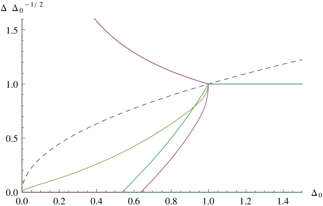
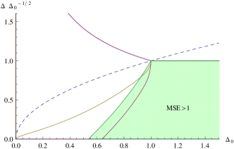
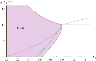
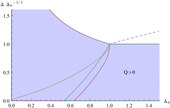
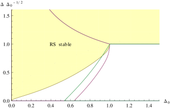
Figure 1: Phase diagram for the planted SK model (rank-one matrix estimation with prior $\pm 1$ with probability $1/2$) with $\Delta_{0}$ being the truth noise variance and $\Delta$ the assume noise variance, obtained solving the SE Eqs. (21)-(23). The dashed line is the Nishimori line $\Delta=\Delta_{0}$. Four different regions are featured: $\text{MSE}>1$, $M>0$, $Q>0$ and the region of RS stability. Note that the Nishimori line lies in the RS stability region. For $\Delta_{0}<1$, the line where $M$ and $Q$ starts to be different from zero (coming from large $\Delta$) corresponds to $\Delta=1$. The line $M=0$ crosses $\Delta=0$ at $\Delta_{0}=2/\pi\sim 0.6366$. The lines $\text{MSE}=1$ intersects the RS stability line at $\Delta_{0}\simeq 0.923$, $\Delta\simeq 0.757$, so that for $0.923\lesssim\Delta_{0}<1$ we have stable solutions with $\text{MSE}>1$.

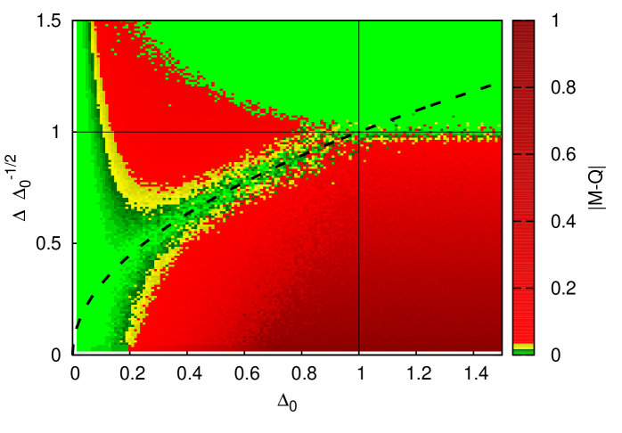
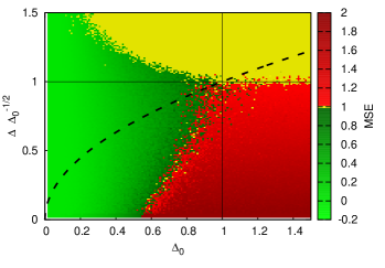
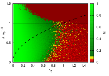
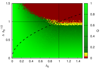
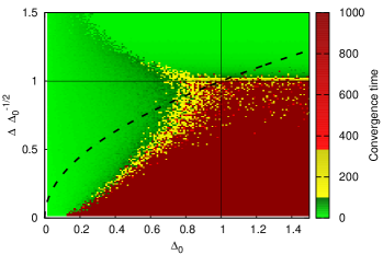
Figure 2: Heat-map of the values obtained running AMP for size $N=5000$ for the planted SK model. The dashed line is the Nishimori line $\Delta=\Delta_{0}$. We show the value of $|M-Q|$ and MSE, $M$, $Q$ and the convergence time. The iterations are stopped when the average change of a variable in a single iteration is less than $10^{-8}$ or at 1000 iterations if convergence is not reached. All is in perfect agreement with the state evolution prediction from Fig. 1.

To illustrate the behaviour of AMP out of the Bayes-optimal case, let us consider the planted Sherrington-Kirkpatrick (SK) model SherringtonKirkpatrick75 , a well-known model both in computer science and physics communities. This is a particular case of the low-rank matrix estimation model Eq. (1) for a bimodal prior, cf. Eq. (8). The output noise is Gaussian with the assumed variance $\Delta$ mismatching the ground-truth variances $\Delta_{0}$, cf. Eqs. (7),(18). In Fig. 1 we show the phase diagram of the model obtained by the SE Eqs. (21)-(23) as $\Delta$ and $\Delta_{0}$ are independently changed. The dashed line is the Nishimori line where the Bayes-optimal condition $\Delta=\Delta_{0}$ holds. For $\Delta_{0}>1$ the signal/noise ratio is too low and the estimation is impossible, $M$ is always zero and $\text{MSE}\geq 1$. Note that a MSE larger than 1 is worse than the error achieved by a random guess from the prior. At $\Delta_{0}=1$, the inference starts to be successful only on the Nishimori line. As one is further and further away from the Nishimori line, the algorithm needs a lower and lower value of noise in order to achieve a positive overlap $M$ and a MSE lower than random guess. In particular, if $\Delta$ is too large, i.e. $\Delta>1$, one always reaches the trivial fixed point $M=Q=0$. The case $\Delta\rightarrow 0$ is also especially meaningful for an evaluation of the MAP estimator Eq. (5). In this case, the value of the overlap with the ground truth $M$ is zero till $\Delta_{0}=2/\pi\sim 0.6366$ NishimoriBook while the MSE is larger than 1 till $\Delta_{0}\simeq 0.55$, almost half than the equivalent threshold on the Nishimori line.

The SE equations describe the average (or large size) behaviour of Low-RAMP and as such they converge in all the phase diagram. Single finite size instances of Low-RAMP do not converge point-wise too far from Nishimori line, cf. Fig. 2.

The analysis of the point-wise convergence on single instances of Low-RAMP can be obtained looking at the Hessian eigenvalues of Low-RAMP equations. A simple way to derive a necessary convergence criterium is to ask whether or not the fixed-point of AMP is stable with respect to weak, infinitesimal, random perturbations. Let us see how it can be derived with the notations of section II.1.4. If we perform, in Eq. (28), the perturbation ${\bf B}^{t}\rightarrow{\bf B}^{t}+{\bm{\epsilon}}^{t}$, where ${\bm{\epsilon}}$ is a i.i.d. infinitesimal vector sampled from ${\cal N}({0,\epsilon})$, then we may ask how this perturbation is carried out at the next step of the iteration. From the recursion (28)-(31), we see that (a) $b^{t+1}$ is not modified to leading order, as $\eta^{\prime}(B+\delta B)=\eta^{\prime}(B)+\delta B\eta^{\prime\prime}(B)$ and the average in (30) makes the perturbation of $O(1/\sqrt{N})$ and (b) ${\bf B}^{t+1}\rightarrow{\bf B}^{t+1}+{\bm{\epsilon}}^{t+1}$ with ${\bm{\epsilon}}^{t+1}=S{\bm{\epsilon}}^{t}\eta^{\prime}({\bf B^{t}})/\sqrt{N}$. The $\ell_{2}$ norm of the perturbation has thus been multiplied, up to a constant ${\mathbb{E}}(S^{2})=\Delta_{0}/\Delta^{2}$, by the empirical average of $\eta^{\prime}({\bf B})$. The fixed-point will be stable if the perturbation does not grow. This yields, coming back to the main notations of the article, to the following criterion:

$$\lambda=1-\frac{\Delta_{0}}{\Delta^{2}}\mathbb{E}_{x^{(0)},W}\left[\left(\frac{\partial^{2}f_{\rm in}(A,B)}{\partial B^{2}}\bigg{|}_{A=\frac{\Delta_{0}}{\Delta^{2}}Q-\frac{\Delta_{0}-\Delta}{\Delta^{2}}\Sigma,\,B=\frac{M}{\Delta}x^{(0)}+\sqrt{\frac{\Delta_{0}Q}{\Delta^{2}}}W}\right)^{2}\right]\,.$$ (35)

For positive $\lambda$ the perturbation decreases and AMP algorithm converges, for negative $\lambda$ it grows and the algorithm does not converge. Interestingly, condition (35) is equivalent to the stability of replica symmetric (RS) solutions in the replica theory given by RS replicon de1978stability (and indeed bolthausen2014iterative has shown rigorously in the SK model, convergence of the AMP algorithm in a phase where the replica symmetric solution is stable). The line where the RS solution becomes unstable (and Low-RAMP stops converging point-wise) is shown in Fig. 1 with a yellow line. Note that, as expected, the RS stability line lies always below the Nishimori line and the two touch at the tri-critical point $\Delta=\Delta_{0}=1$. For small $\Delta_{0}$, the stability line is roughly given by $\Delta\simeq 4\sqrt{\Delta_{0}/(2\pi)}\exp(-1/(2\Delta_{0}))/3$ and it touches the $\Delta=0$ axis only for $\Delta_{0}\rightarrow 0$. This means that for any finite $\Delta_{0}$ the RS solution becomes always unstable for $\Delta$ small enough. The stability line is always above the $M=0$ line, cf. Fig. 1. Note that it is possible to get RS stable solutions with $\text{MSE}>1$: so it is possible that AMP converges point-wise to something worse than random guess.

In Fig. 2 we show the results obtained by running Low-RAMP for single instances of the same problem for $N=5000$. We iterate the Low-RAMP equations, without any damping, for $10^{3}$ steps or we stop when the average change of the variables in a single step of iteration is less than $10^{-8}$. The four regions highlighted in Fig. 1 are well distinguishable. We also show the value of $|M-Q|$, which is zero on the Nishimori line. In particular, it is clear that the point-wise convergence is very fast (less than 100 iterations) well inside the RS stability region, then the convergence time increases rapidly at the boundary of the RS stability region and then stops converging point-wise outside of it.

The scenario illustrated in this section for SK is quite general within low-rank matrix estimation problems. Some differences arise when $x$ is very sparse: in this case on the Nishimori line there is a first order transition LesKrzZde17 and the scenario becomes more complicated, with the coexistence of different phases close to the transition.

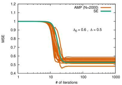
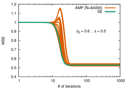
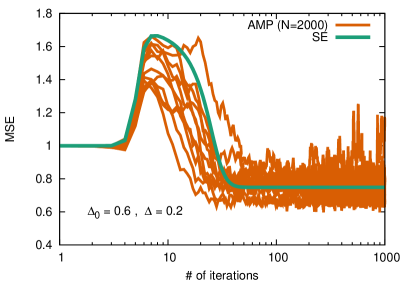
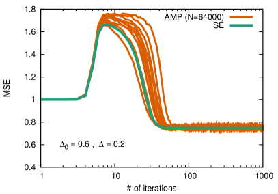
Figure 3: Value of the MSE under iterations of AMP equations for several instances for $N=2000$ (left) and $N=64000$ (right) in the planted SK model with $\Delta_{0}=0.6$ and $\Delta=0.5$ (top), $\Delta=0.2$ (bottom), compared with the SE.

II.3 Optimality and restored Nishimori condition

The Bayes-optimal setting, as reminded in Sec. II.2, is a very special situation: the Nishimori condition Eq. (34) guarantees that the replica symmetry is preserved and that AMP is optimal (in absence of a 1st order phase transition). One consequence of the Nishimori condition is that the typical overlap with the ground truth $M$ and the self-overlap $Q$, as defined in Eqs. (20), are equal. In this case the MSE is then given by

$$\text{MSE}=\mathbb{E}\left[x_{0}^{2}\right]-2M+Q=\mathbb{E}\left[x_{0}^{2}\right]-M\,,$$ (36)

and the minimum MSE is obtained at the maximum overlap $M$. For mismatching models $M$ and $Q$ are typically different from each other and it is not immediate to realize under what conditions the MSE is minimized. We highlighted this property in the main panel of Fig. 2: apart from the trivial solutions $M=Q=0$ (for large $\Delta_{0}$ and $\Delta$) and $M=Q=1$ (for very small $\Delta_{0}$), the overlap with the ground truth $M$ and the self-overlap $Q$ are very close only near the Nishimori line. The Nishimori line is also the region in which AMP is optimal, so it is spontaneous to ask what is the relation (if any) between these two properties in a general setting.

Consider a situation in which we have two or more parameters to tune. These can be parameters in the prior, the variance of the noise $\Delta$ or also the free parameters in the general belief-propagation equations, see for example the parameter $s$ for the ASP algorithm that we will describe in Eqs. (59)-(64). The fundamental question is then for which set of values for the parameters it is possible to obtain optimal estimation error, and how to find them algorithmically. One evident answer is that if all the parameters are chosen to exactly match the values of the ground truth distribution, one ends up on the Nishimori line and then we know that the inference is optimal, and the MSE minimum. But this is not the unique answer.

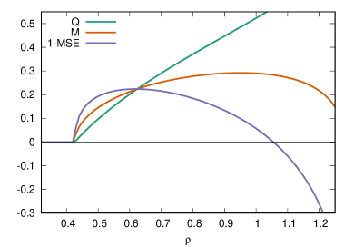
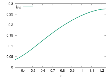
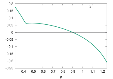
Figure 4: Value of $M$, $Q$ and MSE (top), Bethe free energy $\phi_{\text{RS}}$ (bottom left) and RS stability eigenvalue $\lambda$ (bottom right) as obtained by SE changing the value of $\rho$ in a Rademacher-Bernoulli prior for data generated by a planted SK model with $\Delta_{0}=0.8$ and assuming a noise channel with $\Delta=0.5$. The point where $M=Q$ and the MSE is minimized at $\rho=0.623$.

Let us illustrate what we found with a simple example. The data $Y$ are generated by the planted SK model with $\Delta_{0}=0.8$. In this case the Bayes-optimal inference, knowing the correct prior and noise, would get $\text{MSE}=0.776$. Consider now instead a situation in which one (wrongly!) assumes that the variance of the noise is $\Delta=0.5$ but also, being not sure about the correct prior, assume a more general Rademacher-Bernoulli prior

$$P(x)=\frac{\rho}{2}\delta\left(x-1\right)+\frac{\rho}{2}\delta\left(x+1\right)+\left(1-\rho\right)\delta(x)$$ (37)

with some unknown parameter $\rho$. In Fig. 4 we show the values of $M$, $Q$ and MSE obtained by the SE Eqs. (21)-(23) as a function of $\rho$ while $\Delta$ is kept fixed at $0.5$. Taking $\rho=1$, which corresponds to the correct prior, we obtain $Q\simeq 0.521$, $M\simeq 0.29$ and $\text{MSE}\simeq 0.94$, considerably worse than the Bayes-optimal error. The maximum $M$ is obtained for $\rho\simeq 0.95$, where $Q\simeq 0.48$ and $\text{MSE}\simeq 0.90$. But, if we look to restore the optimality condition $M=Q$, we are led to accept the value $\rho=0.623$: here $M=Q=0.224$ and $\text{MSE}=0.776$, equal to the value obtained by Bayes-optimal inference.

The above observations leads us to a hypothesis: Any combination of the values of parameters that restores the condition $M=Q$, achieves the same performances of the Bayes-optimal setting. We tested this hypothesis in several settings of the low-rank matrix estimation problem, including sparse cases with first order transition LesKrzZde17 . While we always found it true, the underlying reason for this eludes us and is left for future work. The optimality from the restoration of the $M=Q$ condition is relevant in cases in which we assume a wrong functional form of prior, as in the previous example, so that it is indeed impossible to actually reduce to the Bayes-optimal setting.

Note that it is nontrivial to turn the above observation into an algorithmic procedure. A common parameter learning procedure is to maximize the Bethe free energy of the model, Eq. (17). This procedure gives asymptotically the Bayes-optimal parameters, if learning of the exact prior and noise is possible. Nevertheless, if the functional form of the prior and noise is incorrect, this procedure does not return the optimal values of the parameters - that, in our hypothesis, would be the ones associated with the restoration of the $M=Q$ condition. In the previous example, the Bethe free energy is monotonically increasing in $[0,1]$ and has a local maximum only at $\rho\simeq 1.26$, where the prior is not a well-defined probability distribution and the MSE is larger than 1, cf. Fig. 4. It is interesting to look at the RS eigenvalue Eq. (35) for this solution, that is associated with the point-wise convergence of AMP. The eigenvalue is positive for $\rho\lesssim 0.90$, and in particular is positive for the value $\rho\simeq 0.623$, where the optimality condition $M=Q$ is restored. Moreover, for very low $\rho$, in this case for $\rho\lesssim 0.42$, the only solution is the trivial $M=Q=0$, $\text{MSE}=1$. These two extremes give the finite interval $0.42\lesssim\rho\lesssim 0.90$ in which one should indeed look to find the optimal $\rho$. We will discuss further about this observation in Sec. III.3 about the use of ASP.

III The Approximate Survey Propagation: a 1RSB version of AMP

AMP is an established approach to analyze systems with a ferromagnet-like transition, where one expects to have just two possible fixed-points of the iterations. There are, however, situations where there exists a huge number of fixed-points for the AMP equations. In particular, we have shown in the previous section that in the low-rank matrix estimation problem with mismatching models there is a region where the replica symmetry is broken and the AMP algorithm does not converge. In this case one needs to use the cavity method in conjunction with a replica symmetry breaking (RSB) approach, as was introduced by Mézard and Parisi MP01 ; mezard2003cavity ; MPZ02 . In the following we show how this approach can be carried out for the low-rank matrix estimation problem and how this provides a systematic method to deal with mismatching models in a natural way. Note that we need to insist on the notion of independence of the noise elements, that is an essential for belief-propagation-based approaches to work.

III.1 Derivation of the ASP algorithm for the low-rank matrix estimation problem

We derive here the 1-step replica symmetry breaking (1RSB) approximate massage passing, that we call approximate survey propagation (ASP) algorithm, for the low-rank matrix estimation problem. To derive the correct equations in this case, let us consider a replicated inference problem, basically turning the method of Monasson Mo95 into a message passing algorithm. Given the matrix $Y_{ij}$ and $a=1,\ldots,s$, being $s$ the number of real replicas, we assume that

$$Y_{ij}=\frac{x_{i}^{(a)}x_{j}^{(a)}}{\sqrt{N}}+\xi_{ij}^{(a)}\,,$$ (38)

where $\xi_{ij}^{(a)}$ are independent Gaussian noises with zero mean and variance $\Delta$. The partition function becomes

$$Z_{\text{rep}}\left(Y\right)=\int\left[\prod_{a=1}^{s}\prod_{i=1}^{N}\mathrm{d}x_{i}^{(a)}P_{X}(x_{i}^{(a)})\right]\exp\left[\sum_{i\leq j}\sum_{a=1}^{s}g\left(Y_{ij}|w^{(aa)}_{ij}\right)\right]\,,$$ (39)

where $w^{(ab)}_{ij}\equiv x_{i}^{(a)}x_{j}^{(b)}/\sqrt{N}$ and $P_{X}(x)$ and $g$ have the same definition as the previous sections, cf. Eq. (2). If $s=1$ we get back the usual inference problem of Eq. (1).

In order to evaluate the marginals over the variables $\{x_{i}^{(a)}\}$, we need to write the BP equations for the replicated system. In the following let us omit normalization factors when they are irrelevant (they can be determined a posteriori). The BP equations are

$$m_{i\rightarrow ij}(\underline{x}_{i}) \sim\left[\prod_{a=1}^{s}P_{X}(x_{i}^{(a)})\right]\prod_{k\neq j}m_{ki\rightarrow i}(\underline{x}_{i})\,,$$ (40)

$$m_{ij\rightarrow i}(\underline{x}_{i}) \sim\int\mathrm{d}\underline{x}_{j}m_{j\rightarrow ij}(\underline{x}_{j})\exp\left[\sum_{a=1}^{s}g\left(Y_{ij}|w^{(aa)}_{ij}\right)\right]\,,$$ (41)

where we have introduced the notation $\underline{x}_{i}=\{x_{i}^{(1)},\ldots,x_{i}^{(s)}\}$. This follows directly from the factor graph represented in Fig. 5.

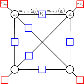
Figure 5: The factor graph representing the structure of the replicated posterior measure whose partition function is described in Eq. (39). The variable nodes are replicated variables $\underline{x}_{i}\equiv\{x_{i}^{(1)},\ldots,x_{i}^{(s)}\}$.

At this point we introduce a 1RSB parametrization for the cavity distributions

$$m_{j\rightarrow ij}(\underline{x}_{j})\sim\int\mathrm{d}h\,\exp\left[-\frac{1}{2\Delta^{(0)}_{j\rightarrow ij}}\left(h-\hat{x}_{j\rightarrow ij}\right)^{2}\right]\prod_{a=1}^{s}\exp\left[-\frac{1}{2\Delta^{(1)}_{j\rightarrow ij}}\left(x_{j}^{(a)}-h\right)^{2}\right]\>.$$ (42)

The form of this ansatz elucidates why we are considering a replicated system: if the posterior measure Eq. (2) develops a 1RSB structure, the phase space of the solutions of the inference problem gets clustered in exponentially many basins of solutions MPV87 . Therefore, if we consider a set of $s$ real copies of the same inference problem and we infinitesimally couple them, they will acquire a finite probability to fall inside the same cluster of solutions. This line of reasoning is exactly the same as the one considered to describe the real replica approach for glasses Mo95 ; CKPUZ17 and the ansatz of Eq. (42) reproduces the infinite dimensional caging ansatz (at the 1RSB level) for hard spheres in infinite dimension CKPUZ14 ; CKPUZ13 .

The ansatz of Eq. (42) allows for three relevant correlation functions

$$\left\langle x_{j}^{(a)}\right\rangle =\hat{x}_{j\rightarrow ij}\,,$$

$$\left.\left\langle x_{j}^{(a)}x_{j}^{(b),\top}\right\rangle\right|_{a\neq b} =\Delta_{j\rightarrow ij}^{(0)}+\hat{x}_{j\rightarrow ij}\,\hat{x}_{j\rightarrow ij}^{\top}\,,$$ (43)

$$\left\langle x_{j}^{(a)}x_{j}^{(a),\top}\right\rangle =\Delta_{j\rightarrow ij}^{(1)}+\Delta_{j\rightarrow ij}^{(0)}+\hat{x}_{j\rightarrow ij}\,\hat{x}_{j\rightarrow ij}^{\top}\,,$$

where the averages are taken with the measure defined in Eq. (42). The last two lines give access to the correlation between cavity messages from one copy to another. Note that if $\Delta^{(0)}_{j\rightarrow ij}=0$ different replicas become uncorrelated. Therefore in the limit $\Delta^{(0)}_{j\rightarrow ij}\rightarrow 0$ one recovers the replica symmetric AMP. Equivalently, if one fixes $s=1$ the ansatz reduces naturally to the RS parametrization for the cavity messages and one gets back again to the AMP algorithm.

Given the 1RSB ansatz, we can plug Eq. (42) in Eq. (41) to get

$$m_{ij\rightarrow i}(\underline{x}_{i})\sim \int\mathrm{d}he^{-\frac{1}{2\Delta^{(0)}_{j\rightarrow ij}}\left(h-\hat{x}_{j\rightarrow ij}\right)^{2}}\prod_{a=1}^{s}\int\mathrm{d}x_{j}^{(a)}\exp\left[-\frac{1}{2\Delta^{(1)}_{j\rightarrow ij}}\left(x_{j}^{(a)}-h\right)^{2}+g\left(Y_{ij}|w^{(ab)}\right)\right]$$

$$\sim \exp\left[\frac{1}{\sqrt{N}}S_{ij}\hat{x}_{j\rightarrow ij}\sum_{a=1}^{s}x_{j}^{(a)}-\frac{1}{2N}\hat{R}_{ij}\left(\Delta^{(1)}_{j\rightarrow ij}\Delta^{(0)}_{j\rightarrow ij}+\left(\hat{x}_{j\rightarrow ij}\right)^{2}\right)\sum_{a=1}^{s}\left(x_{j}^{(a)}\right)^{2}\right.$$

$$\qquad+\left.\frac{1}{2N}S_{ij}^{2}\Delta^{(0)}_{j\rightarrow ij}\left(\sum_{a=1}^{s}x_{j}^{(a)}\right)^{2}+\frac{1}{2N}S_{ij}^{2}\Delta^{(1)}_{j\rightarrow ij}\sum_{a=1}^{s}\left(x_{j}^{(a)}\right)^{2}\right]\,,$$ (44)

where the matrices $S_{ij}$ and $\hat{R}_{ij}$ are the same as introduced in Eq. (7). Plugging this result inside the first one of Eqs. (41) we get

$$m_{i\rightarrow ij}(\underline{x}_{i})\sim\left[\prod_{a=1}^{s}P_{X}(x_{i}^{(a)})\right]\exp\left[T_{i\rightarrow ij}\sum_{a=1}^{s}x_{i}^{(a)}-\frac{1}{2}V_{i\rightarrow ij}^{(1)}\sum_{a=1}^{s}\left(x_{i}^{(a)}\right)^{2}+\frac{1}{2}V_{i\rightarrow ij}^{(0)}\left(\sum_{a=1}^{s}x_{i}^{(a)}\right)^{2}\right]\,,$$

where we have defined

$$T_{i\rightarrow ij} =\frac{1}{\sqrt{N}}\sum_{k\neq j}S_{ik}\hat{x}_{k\rightarrow ik}\,,$$ (45)

$$V^{(1)}_{i\rightarrow ij} =\frac{1}{N}\sum_{k\neq j}\left[\hat{R}_{ik}\left(\Delta^{(1)}_{k\rightarrow ik}+\Delta^{(0)}_{k\rightarrow ik}+\left(\hat{x}_{k\rightarrow ik}\right)^{2}\right)-S_{ik}^{2}\Delta_{k\rightarrow ik}^{(1)}\right]\,,$$ (46)

$$V^{(0)}_{i\rightarrow ij} =\frac{1}{N}\sum_{k\neq j}S_{ik}^{2}\Delta_{k\rightarrow ik}^{(0)}\>.$$ (47)

We can now close the equations. We have

$$\left\langle x_{i}^{(a)}\right\rangle =\frac{1}{s}\frac{\partial}{\partial T_{i\rightarrow ij}}f_{\text{in}}\left[T_{i\rightarrow ij},V^{(1)}_{i\rightarrow ij},V^{(0)}_{i\rightarrow ij}\right]\,,$$ (48)

$$\left\langle\left(x_{i}^{(a)}\right)^{2}\right\rangle =-\frac{2}{s}\frac{\partial}{\partial V^{(1)}_{i\rightarrow ij}}f_{\text{in}}\left[T_{i\rightarrow ij},V^{(1)}_{i\rightarrow ij},V^{(0)}_{i\rightarrow ij}\right]\,,$$ (49)

$$\left\langle x_{i}^{(a)}x_{i}^{(b)}\right\rangle =\frac{2}{s(s-1)}\left[\frac{\partial}{\partial V_{i\rightarrow ij}^{(0)}}+\frac{\partial}{\partial V_{i\rightarrow ij}^{(1)}}\right]f_{\text{in}}\left[T_{i\rightarrow ij},V^{(1)}_{i\rightarrow ij},V^{(0)}_{i\rightarrow ij}\right]\,,$$ (50)

where we have introduced the function

$$f_{\text{in}}\left[T,V^{(1)},V^{(0)}\right] =\ln\int\mathrm{d}\underline{x}\left[\prod_{a=1}^{s}P_{X}(x^{(a)})\right]\exp\left[T\sum_{a=1}^{s}x^{(a)}-\frac{1}{2}V^{(1)}\sum_{a=1}^{s}\left(x_{i}^{(a)}\right)^{2}+\frac{1}{2}V^{(0)}\left(\sum_{a=1}^{s}x_{i}^{(a)}\right)^{2}\right]$$

$$=\ln\int\mathrm{d}he^{-\frac{1}{2}V^{(0)}h^{2}}\sqrt{\frac{V^{(0)}}{2\pi}}\left\{\int\mathrm{d}xP_{X}(x)\exp\left[-\frac{1}{2}V^{(1)}x^{2}+(T+V^{(0)}h)x\right]\right\}^{s}\>.$$ (51)

Using Eqs. (43), we obtain

$$\hat{x}_{i\rightarrow ij} =\frac{1}{s}\frac{\partial}{\partial T_{i\rightarrow ij}}f_{\text{in}}\left[T_{i\rightarrow ij},V^{(1)}_{i\rightarrow ij},V^{(0)}_{i\rightarrow ij}\right]\,,$$ (52)

$$\Delta^{(0)}_{i\rightarrow ij} =\frac{2}{s(s-1)}\left[\frac{\partial}{\partial V^{(1)}_{i\rightarrow ij}}+\frac{\partial}{\partial V^{(0)}_{i\rightarrow ij}}\right]f_{\text{in}}\left[T_{i\rightarrow ij},V^{(1)}_{i\rightarrow ij},V^{(0)}_{i\rightarrow ij}\right]-\frac{1}{s^{2}}\left(\frac{\partial}{\partial T_{i\rightarrow ij}}f_{\text{in}}\left[T_{i\rightarrow ij},V^{(1)}_{i\rightarrow ij},V^{(0)}_{i\rightarrow ij}\right]\right)^{2}\,,$$ (53)

$$\Delta^{(1)}_{i\rightarrow ij} =2\left[\frac{1}{s(1-s)}\left(\frac{\partial}{\partial V^{(1)}_{i\rightarrow ij}}+\frac{\partial}{\partial V^{(0)}_{i\rightarrow ij}}\right)-\frac{1}{s}\frac{\partial}{\partial V^{(1)}_{i\rightarrow ij}}\right]f_{\text{in}}\left[T_{i\rightarrow ij},V^{(1)}_{i\rightarrow ij},V^{(0)}_{i\rightarrow ij}\right]\>.$$ (54)

The Eqs. (52)-(54) together with Eqs. (45)-(47) constitute the 1RSB-BP equations, within the Gaussian ansatz of Eq. (42), and with Parisi parameter $s$.

Finally, the moments of the marginal distributions are obtained by introducing

$$T_{i} =\frac{1}{\sqrt{N}}\sum_{k}S_{ik}\hat{x}_{k\rightarrow ik}\,,$$ (55)

$$V^{(1)}_{i} =\frac{1}{N}\sum_{k}\left[\hat{R}_{ik}\left(\Delta^{(1)}_{k\rightarrow ik}+\Delta^{(0)}_{k\rightarrow ik}+\left(\hat{x}_{k\rightarrow ik}\right)^{2}\right)-S_{ik}^{2}\Delta_{k\rightarrow ik}^{(1)}\right]\,,$$ (56)

$$V^{(0)}_{i} =\frac{1}{N}\sum_{k}S_{ik}^{2}\Delta_{k\rightarrow ik}^{(0)}\,,$$ (57)

through which we have

$$\hat{x}_{i}\equiv\frac{1}{s}\sum_{a=1}^{s}\left[x_{i}^{(a)}\right]= \frac{1}{s}\frac{\partial}{\partial T_{i}}f_{\text{in}}\left[T_{i},V^{(1)}_{i},V^{(0)}_{i}\right]\,,$$

$$\left.\left[x_{i}^{(a)}x_{i}^{(b)}\right]\right|_{a\neq b}-\hat{x}_{i}^{2}=\Delta^{(0)}_{i}= \frac{2}{s(s-1)}\left[\frac{\partial}{\partial V^{(1)}_{i}}+\frac{\partial}{\partial V^{(0)}_{i}}\right]f_{\text{in}}\left[T_{i},V^{(1)}_{i},V^{(0)}_{i}\right]$$

$$-\frac{1}{s^{2}}\left(\frac{\partial f_{\text{in}}\left[T_{i},V^{(1)}_{i},V^{(0)}_{i}\right]}{\partial T_{i}}\right)^{2}\,,$$ (58)

$$\left[\left(x_{i}^{(a)}\right)^{2}\right]-\left.\left[x_{i}^{(a)}x_{i}^{(b)}\right]\right|_{a\neq b}=\Delta^{(1)}_{i}= 2\left[\frac{1}{s(1-s)}\left(\frac{\partial}{\partial V^{(1)}_{i}}+\frac{\partial}{\partial V^{(0)}_{i}}\right)-\frac{1}{s}\frac{\partial}{\partial V^{(1)}_{i}}\right]f_{\text{in}}\left[T_{i},V^{(1)}_{i},V^{(0)}_{i}\right]\,,$$

where the square brackets $\left[\cdot\right]$ indicate the average over the replicated posterior measure defined in Eq. (39). The complexity of the 1RSB-BP algorithm described in Eqs. (45)-(47), (52)-(54) can be reduced by working directly with the moments of the real marginals instead using the moments of the cavity marginals. This TAPification procedure is well known in inference problems (cf. Sec. II.1.1 and references therein). The result is the ASP algorithm for the low-rank matrix estimation problem:

$$T_{i}^{t}= \frac{1}{\sqrt{N}}\sum_{k}S_{ik}\hat{x}_{k}^{t}-\frac{1}{N}\hat{x}_{i}^{t-1}\sum_{k}S_{ik}^{2}\left(\Delta^{(1),t}_{k}+s\Delta^{(0),t}_{k}\right)\,,$$ (59)

$$V^{(1),t}_{i}= \frac{1}{N}\sum_{k}\left[\hat{R}_{ik}\left(\Delta^{(1),t}_{k}+\Delta^{(0),t}_{k}+\left(\hat{x}_{k}^{t}\right)^{2}\right)-S_{ik}^{2}\Delta_{k}^{(1),t}\right]\,,$$ (60)

$$V^{(0),t}_{i}= \frac{1}{N}\sum_{k}S_{ik}^{2}\Delta_{k}^{(0),t}\,,$$ (61)

$$\hat{x}_{i}^{t+1}= \frac{1}{s}\frac{\partial}{\partial T_{i}}f_{\text{in}}\left[T_{i}^{t},V^{(1),t}_{i},V^{(0),t}_{i}\right]\,,$$ (62)

$$\Delta^{(0),t+1}_{i}= \frac{2}{s(s-1)}\left[\frac{\partial}{\partial V^{(1)}_{i}}+\frac{\partial}{\partial V^{(0)}_{i}}\right]f_{\text{in}}\left[T_{i}^{t},V^{(1),t}_{i},V^{(0),t}_{i}\right]-\frac{1}{s^{2}}\left(\frac{\partial f_{\text{in}}\left[T_{i}^{t},V^{(1),t}_{i},V^{(0),t}_{i}\right]}{\partial T_{i}}\right)^{2}\,,$$ (63)

$$\Delta^{(1),t+1}_{i}= 2\left[\frac{1}{s(1-s)}\left(\frac{\partial}{\partial V^{(1)}_{i}}+\frac{\partial}{\partial V^{(0)}_{i}}\right)-\frac{1}{s}\frac{\partial}{\partial V^{(1)}_{i}}\right]f_{\text{in}}\left[T_{i}^{t},V^{(1),t}_{i},V^{(0),t}_{i}\right]\,.$$ (64)

Strictly speaking we have different algorithms for different values of the Parisi parameter $s$. We will comment more about the use of this parameter in Sec. II.3. Note that for $s=1$ the equations depend only on $\sigma_{i}=\Delta^{(1)}_{i}+\Delta^{(0)}_{i}$ and the algorithm reduces to the Low-RAMP Eqs. (9)-(12) with $B_{i}=T_{i}$ and $A_{i}=V^{(1)}-V^{(0)}$. Observe also that, similarly to what happens in Low-RAMP, the equations can be further simplified replacing $S_{ij}^{2}$ by its mean, without changing the leading order in $N$. This simplification allows to express Eqs. (59)-(61) simply as matrix multiplications, cf. Sec. III.2.2. The introduction of a RSB structure in the algorithm allows ASP to converge point-wise and to obtain a low MSE also in regions where the RS solution is unstable and AMP does not converge point-wise, cf. Fig. 6.

The fixed-points of the ASP equations are stationary points of the following free energy:

$$\Phi^{\text{1RSB}}_{\text{Bethe}}= \max_{T_{i},V^{(0)}_{i},V^{(1)}_{i}}\sum_{1\leq i\leq N}\frac{1}{s}f_{\text{in}}\left(T_{i},V^{(0)}_{i},V^{(1)}_{i}\right)-T_{i}\hat{x}_{i}+\frac{1}{2}\left(V^{(1)}_{i}-V^{(0)}_{i}\right)\Delta^{(1)}_{i}+\frac{1}{2}\left(V^{(1)}_{i}-sV^{(0)}_{i}\right)\left(\hat{x}_{i}^{2}+\Delta^{(0)}_{i}\right)$$

$$+\frac{1}{2}\sum_{1\leq i,j\leq N}\biggl{\{}\frac{S_{ij}}{\sqrt{N}}\hat{x}_{i}\hat{x}_{j}-\frac{\hat{R}_{ij}}{2N}\left(\hat{x}_{i}^{2}+\Delta^{(1)}_{i}+\Delta^{(0)}_{i}\right)\left(\hat{x}_{j}^{2}+\Delta^{(1)}_{j}+\Delta^{(0)}_{j}\right)+$$

$$\qquad\qquad\qquad+\frac{S_{ij}^{2}}{2N}\left[2\hat{x}_{i}^{2}\left(\Delta^{(1)}_{j}+s\Delta^{(0)}_{j}\right)-\left(\Delta^{(1)}_{i}+s\Delta^{(0)}_{i}\right)\left(\Delta^{(1)}_{j}+s\Delta^{(0)}_{j}\right)\right]\biggl{\}}$$ (65)

This free energy is known in statistical physics literature as the 1RSB potential and is useful to compare different fixed-points at same $s$, in the same spirit of the RS case. Note that when one tries to compare fixed-points of ASP that are associated to different values of $s$, the extremization of this free energy does not correspond to the minimum MSE, cf. Sec. III.3.

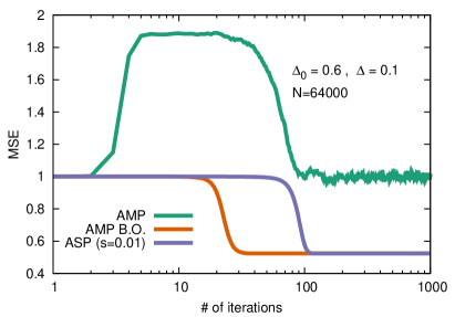
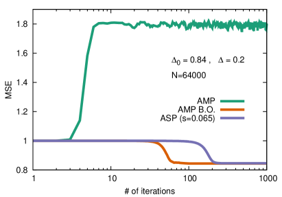
Figure 6: MSE under iterations of ASP for $N=64000$ in the planted SK model with $\Delta_{0}=0.6$, $\Delta=0.1$, $s=0.01$ (left) and $\Delta_{0}=0.84$, $\Delta=0.2$, with $s=0.065$ (right). We compare ASP with AMP run on the same data with the same $\Delta$ as ASP (green lines) and AMP run in the Bayes-optimal setting $\Delta=\Delta_{0}$ (orange lines). In these situations, well inside the RS instability region, AMP does not converge point-wise and the associated MSE is typically equal or larger than 1. The ASP algorithm instead converges point-wise with a MSE close to the AMP run in the Bayes-optimal setting ($\Delta=\Delta_{0}$), at least for some value of $s$, cf. Sec. III.3.

III.2 The 1RSB state evolution equations

The ASP algorithm can be implemented on a single instance of the inference problem. Moreover, in the same lines as for AMP (cf. Sec. II.1.3) it is possible to obtain the state evolution equations for ASP. One assumes that $Y$ is generated through the process of first extracting the signal $\{x_{i}^{(0)}\}$ from a probability distribution $P_{0}(\{x_{i}^{(0)}\})=\prod_{i=1}^{N}P_{0}(x_{i}^{(0)})$ and, then, it is measured through a Gaussian channel of zero mean and variance $\Delta_{0}$ so that $P(Y_{ij})=\exp\left[g^{(0)}\left(Y_{ij}|w_{ij}^{(0)}\right)\right]$ with $g^{(0)}(Y|w)$ given in Eq. (18). Once again, central limit theorem assures that the average over $Y$ of the variables $T_{i}$ of Eq. (59) become Gaussian with

$$\overline{T_{i}^{t}} =\frac{M^{t}}{\Delta}x_{i}^{(0)}\,, \overline{\left(T_{i}^{t}\right)^{2}} =\frac{\Delta_{0}}{\Delta^{2}}Q^{t}+\left(\frac{M^{t}}{\Delta}x_{i}^{(0)}\right)^{2}\,,$$ (66)

where $M$ and $Q$ are the usual order parameters (cf. Eq. (20))

$$M^{t}=\frac{1}{N}\sum_{k=1}^{N}\hat{x}_{k}^{t}x_{k}^{(0)}\,, Q^{t}=\frac{1}{N}\sum_{k=0}^{N}\left(\hat{x}_{k}^{t}\right)^{2}\>.$$ (67)

Instead $V_{i}^{(1)}$ and $V_{i}^{(0)}$, as defined in Eq. (60)-(61), at leading order in $N$ are concentrated around their mean value

$$V^{(0),t}=\overline{V_{i}^{(0),t}}=\frac{\Delta_{0}}{\Delta^{2}}\Delta^{(0),t}\,, V^{(1),t}=\overline{V_{i}^{(1),t}}=\frac{1}{\Delta}\left(\Delta^{(1),t}+\Delta^{(0),t}+Q^{t}\right)-\frac{\Delta_{0}}{\Delta^{2}}\Delta^{(1),t}\,,$$ (68)

and we have defined the order parameters

$$\Delta^{(0),t}=\frac{1}{N}\sum_{k=1}^{N}\Delta_{k}^{(0),t}\,, \Delta^{(1),t}=\frac{1}{N}\sum_{k=1}^{N}\Delta_{k}^{(1),t}\>.$$ (69)

Starting from this, the parameters $M$, $Q$, $\Delta^{(1)}$ and $\Delta^{(0)}$ are fixed self-consistently using Eqs. (62)-(64). Let us consider $M$. From Eq. (62) we get that

$$M^{t+1}= \frac{1}{N}\int\left[\prod_{i=1}^{N}\mathrm{d}x_{i}^{(0)}P_{0}\left(x^{(0)}_{i}\right)\right]\left(\sum_{k=1}^{N}\hat{x}_{k}^{t+1}\,x_{k}^{(0)}\right)$$

$$= \frac{1}{s}\int\mathrm{d}\underline{x}^{(0)}P_{0}(\underline{x}^{(0)})\cdot$$ (70)

$$\cdot\left.\frac{\partial}{\partial T}f_{\text{in}}\int\frac{\mathrm{d}w}{\sqrt{2\pi}}e^{-w^{2}/2}\left[T^{t},\frac{1}{\Delta}\left(\Delta^{(1),t}+\Delta^{(0),t}+Q^{t}\right)-\frac{\Delta_{0}}{\Delta^{2}}\Delta^{(1),t},\,\frac{\Delta_{0}}{\Delta^{2}}\Delta^{(0),t}\right]\right|_{T=\frac{M^{t}}{\Delta}x^{(0)}+\sqrt{\frac{\Delta_{0}}{\Delta^{2}}Q^{t}}W}\>.$$

Therefore, defining

$${\mathbb{E}}_{x^{(0)},W}(A)=\int\frac{\mathrm{d}W}{\sqrt{2\pi}}e^{-W^{2}/2}\int\mathrm{d}\underline{x}^{(0)}P_{0}(\underline{x}^{(0)})A\>$$ (71)

and

$$T^{t} =\frac{M^{t}}{\Delta}x^{(0)}+\sqrt{\frac{\Delta_{0}Q^{t}}{\Delta^{2}}}W\,,$$ (72)

$$V^{(1),t} =\frac{1}{\Delta}\left(\Delta^{(1),t}+\Delta^{(0),t}+Q^{t}\right)-\frac{\Delta_{0}}{\Delta^{2}}\Delta^{(1),t}\,,$$ (73)

$$V^{(0),t} =\frac{\Delta_{0}}{\Delta^{2}}\Delta^{(0),t}\,,$$ (74)

one can rewrite Eq. (70) as

$$M^{t+1}=\frac{1}{s}{\mathbb{E}}_{x^{(0)},W}\left[\frac{\partial}{\partial T}f_{\text{in}}\left[T^{t},V^{(1),t},V^{(0),t}\right]\,x^{(0)}\right]\,.$$ (75)

Using Eqs. (63)-(64) and the definitions given in Eq. (67)-(69) one gets similarly

$$Q^{t+1} =\frac{1}{s^{2}}{\mathbb{E}}_{x^{(0)},W}\left[\left(\frac{\partial}{\partial T}f_{\text{in}}\left[T^{t},V^{(1),t},V^{(0),t}\right]\right)^{2}\right]\,,$$ (76)

$$\Delta^{(0),t+1} ={\mathbb{E}}_{x^{(0)},W}\left[\frac{2}{s(s-1)}\left[\frac{\partial}{\partial V^{(1)}}+\frac{\partial}{\partial V^{(0)}}\right]f_{\text{in}}\left[T^{t},V^{(1),t},V^{(0),t}\right]-\frac{1}{s^{2}}\left(\frac{\partial f_{\text{in}}\left[T^{t},V^{(1),t},V^{(0),t}\right]}{\partial T}\right)^{2}\right]\,,$$ (77)

$$\Delta^{(1),t+1} ={\mathbb{E}}_{x^{(0)},W}\left[2\left[\frac{1}{s(1-s)}\left(\frac{\partial}{\partial V^{(1)}}+\frac{\partial}{\partial V^{(0)}}\right)-\frac{1}{s}\frac{\partial}{\partial V^{(1)}}\right]f_{\text{in}}\left[T^{t},V^{(1),t},V^{(0),t}\right]\right]\,,$$ (78)

that are the state evolution equations of ASP, or 1RSB-SE. The solution of the state evolution equations coincides with the result of the replica theory for the 1RSB structure provided $\Delta^{(0)}=q_{1}-q_{0}$ , $Q=q_{0}$ and $\Delta^{(1)}=q_{d}-q_{1}$ (cf. Appendix A). The 1RSB-SE provides the typical asymptotic behaviour of ASP. In Fig. 7 we show how single instances of ASP converge to the 1RSB-SE for large sizes.

Note that we derived the 1RSB eqs. (75-78) as a state evolution of the ASP algorithm without using the replica trick in any way. We used the aid of real replicas in the derivation of the ASP algorithm, but we could have simply postulated the algorithm and derive (or prove, see section III.2.2) its state evolution anyway. Our approach thus provides a concrete algorithmic meaning to the 1RSB equations, that can be understood independently of the replica method. The advantage of this algorithmic interpretation is that the ASP algorithm follows its state evolution even if the statistical properties of the model are not described by 1RSB.

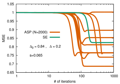
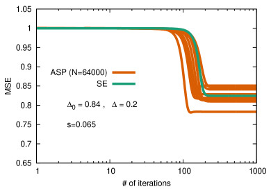
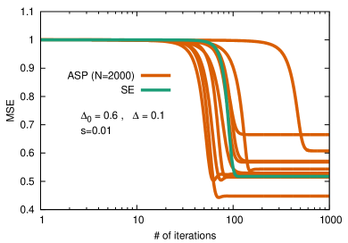
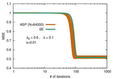
Figure 7: Iterations of ASP for system sizes $N=2000$ (left) and $N=64000$ (right) compared with SE for the planted SK model with $\Delta_{0}=0.84$, $\Delta=0.2$, $s=0.065$ (top) and $\Delta_{0}=0.6$, $\Delta=0.1$, $s=0.01$ (bottom). Note that for these values of $\Delta_{0}$ and $\Delta$ we are in the region where RS solution is unstable, cf. Fig. 1.

III.2.1 The 1RSB free energy and complexity

The algorithmic interpretation of the 1RSB is not limited to the fixed point equations, but concerns the free energy as well. In the same way AMP can be interpreted as extremizing the replica symmetric Bethe free energy (17), ASP can be interpreted as extremizing the 1RSB Bethe free energy (65).

The 1RSB-SE equations corresponds to the stationary points of the free energy, which we give here without derivation, as it can readily be adapted from the RS one:

$$\Phi_{\text{1RSB}}=\max\left\{\phi_{\text{1RSB}}\left(M,Q,\Delta^{(0)},\Delta^{(1)}\right),\frac{\partial\phi_{\text{1RSB}}}{\partial M}=\frac{\partial\phi_{\text{1RSB}}}{\partial Q}=\frac{\partial\phi_{\text{RS}}}{\partial\Delta^{(0)}}=\frac{\partial\phi_{\text{RS}}}{\partial\Delta^{(1)}}=0\right\}$$ (79)

with

$$\phi_{\text{1RSB}}\left(M,Q,\Delta^{(0)},\Delta^{(1)}\right)= s\frac{\Delta_{0}}{4\Delta^{2}}Q^{2}-\frac{1}{2\Delta}M^{2}-\frac{\Delta_{0}-\Delta}{4\Delta^{2}}\left(Q+\Delta^{(0)}+\Delta^{(1)}\right)^{2}+$$

$$+(1-s)\frac{\Delta_{0}}{4\Delta^{2}}\left(Q+\Delta^{(0)}\right)^{2}+\frac{1}{s}{\mathbb{E}}_{x^{(0)},W}\left[f_{\text{in}}\left(T,V^{(0)},V^{(1)}\right)\right]\,,$$ (80)

where $T$, $V^{(0)}$ and $V^{(1)}$ are functions of the order parameters as for Eqs. (72)-(74). This free energy coincides with the one obtained by replica theory under 1RSB ansatz and reduces to Eq. (26) for $s=1$. From the previous expression one can obtain the value of $s$ that extremizes the free energy. From the point of view of physics, this value of $s$ would be the one that describes the equilibrium states of the system in a 1RSB phase. From the point of view of inference, this value of $s$ does not minimizes the MSE, as we discuss in Sec. III.3.

In the case the posterior measure develops a 1RSB structure, the phase space of configurations becomes clustered in exponentially many basins. In this situation, the number of basins is counted by the complexity MPV87 . The complexity $\Sigma$ as function of the free energy of a single metastable state can be obtained as the Legendre transform of the 1RSB free energy of the system, obtaining

$$\Sigma\left(M,Q,\Delta^{(0)},\Delta^{(1)}\right)= s^{2}\frac{\Delta_{0}}{4\Delta^{2}}\Delta^{(0)}\left(2Q+\Delta^{(0)}\right)-s^{2}\frac{\partial}{\partial s}{\mathbb{E}}_{x^{(0)},W}\left[\frac{1}{s}f_{\text{in}}\left(T,V^{(0)},V^{(1)}\right)\right]$$ (81)

From the point of view of physics, the static solution corresponds to the metastable states with the lowest free energy and null complexity. The inclusion of the 1RSB structure in ASP allows to analyze situations with nonzero complexity $\Sigma$.

III.2.2 Rigorous approach reloaded

Interestingly, we can use the rigorous result for state evolution of AMP from Sec. II.1.4 in the present context as well, and show that ASP follows rigorously a state evolution corresponding to the 1RSB equations.

Theorem 2 (State Evolution for Approximate Survey Propagation).

For the ASP algorithm, the empircal averages

$$M^{t} =\frac{1}{N}\sum_{i}\hat{x}^{t}_{i}x^{(0)}_{i}\,, Q^{t} =\frac{1}{N}\sum_{i}(\hat{x}^{t}_{i})^{2}\,, \Psi^{t} =\frac{1}{N}\sum_{i}\psi(B_{i}^{t},x^{(0)}_{i})\,,$$ (82)

for a large class of function $\psi$ (see deshpande2015asymptotic ) converge, when $N\rightarrow\infty$, to their state evolution predictions where

$$M_{\rm SE}^{t} =\mathbb{E}\left[x^{0}\eta_{t}(Z)\right]\,, Q^{t}_{\rm SE} =\mathbb{E}\left[\eta_{t}(Z)^{2}\right]\,, \Psi^{t}_{\rm SE} =\mathbb{E}\left[\psi(Z,x^{(0)})\right]\,,$$ (83)

where $Z$ is a random Gaussian variable with mean $\frac{M^{t}x^{(0)}}{\Delta}$ and variance $\frac{\Delta Q^{t}}{\Delta^{2}}$, and $x^{(0)}$ is distributed according to the prior $P_{0}$.

Proof.

First, let us rewrite the ASP algorithm in a AMP-like form as considered in DeshpandeM14 ; deshpande2015asymptotic

$${\bf T}^{t}= \frac{1}{\sqrt{N}}S\hat{\bf x}^{t}-b^{t}\hat{\bf x}^{t-1}\,,$$ (84)

$$\hat{x}_{i}^{t+1}= \eta_{t}({T}_{i}^{t})\,,$$ (85)

with, again

$$b^{t}=\frac{{\mathbb{E}}[S^{2}]}{N}\sum_{i=1}^{N}(\partial_{T}\eta_{t}({T}_{i}^{t}))\,.$$ (86)

With the particular choice of the following denoising function

$$\eta_{t}({T}_{i}^{t})=\vcentcolon\frac{1}{s}\frac{\partial}{\partial T_{i}}f_{\text{in}}\left[T_{i}^{t},V^{(1),t},V^{(0),t}\right]$$ (87)

where $V^{(1),t}$, $V^{(1),t}$ are deterministic variables given by eqs. (73-74) with use of eqs. (77-78). Once ASP is written in this form, we can apply directly theorem 1 from section II.1.4 and reach the desired result. ∎

III.3 Behaviour and performance of ASP

The ASP algorithm is a natural generalization of AMP, taking into account the 1-step replica symmetry broken structure in place of a replica symmetry. In this section we discuss the performance of ASP in terms of its convergence and estimation error it reaches as a function of the Parisi parameter $s$. We recall that for $s=1$ the ASP algorithm reduces to AMP. We illustrate our findings again on the SK model. We compare the performance of the algorithm on finite size instances with the fixed-points of 1RSB-SE Eqs. (75)-(78).

III.3.1 MSE as a function of the Parisi parameter $s$

The most interesting quantity from the inference point of view is the mean-squared error reached by the ASP algorithm for different values of the Parisi parameter $s$. In Fig. 8 we show the MSE for the planted SK model for two values of $\Delta_{0}$ (the two panels) as a function of $\Delta$ for various values of the Parisi parameter $s$.

First we note that in the whole region of convergence of AMP, i.e. in the RS stability region, ASP converges for every value of $s$ to the same fixed point as AMP, cf. Fig. 8. In this sense, ASP provides a strong test (on a single instance) of the replica symmetry of the problem: if ASP converges to the same fixed point for any value of $s$, we have an argument to claim replica symmetry (in absence of discontinuous phase transitions).

The horizontal line in Fig. 8 is the optimal MSE reached by AMP in the Bayes-optimal case where $\Delta=\Delta_{0}$. The black line corresponds to the MSE reached for the equilibrium value of $s^{*}(\Delta)$ for which the complexity Eq. (81) vanishes, or equivalently where the free energy Eq. (80) is maximized. These are the states dominating the Boltzmann measure if 1RSB was the correct description of the system (which it is not in this model, as well known and explained in the next section).

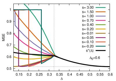
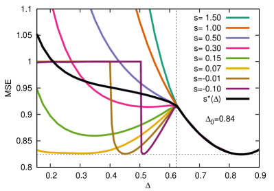
Figure 8: Mean-squared error as extracted from the solution of 1RSB SE Eqs. (75)-(78) for SK model with $\Delta_{0}=0.6$ (left) and $\Delta_{0}=0.84$ (right) varying $\Delta$ and for several $s$. For large $\Delta$ (on the right of the vertical dotted line) the RS solution is stable and ASP converges to the same solution for any $s$. For small $\Delta$ (on the left of the vertical dotted line) the RS solution is unstable, AMP stops converging point-wise and ASP gives different solutions varying $s$. We plot also the value of MSE obtained by ASP when $s$ is fixed to $s^{*}(\Delta)$, defined as the value of $s$ that maximizes the Bethe free energy Eq. (80). Note that in some cases the MSE obtained by ASP in the RSB region is indistinguishable from the optimal one obtained for $\Delta=\Delta_{0}$.

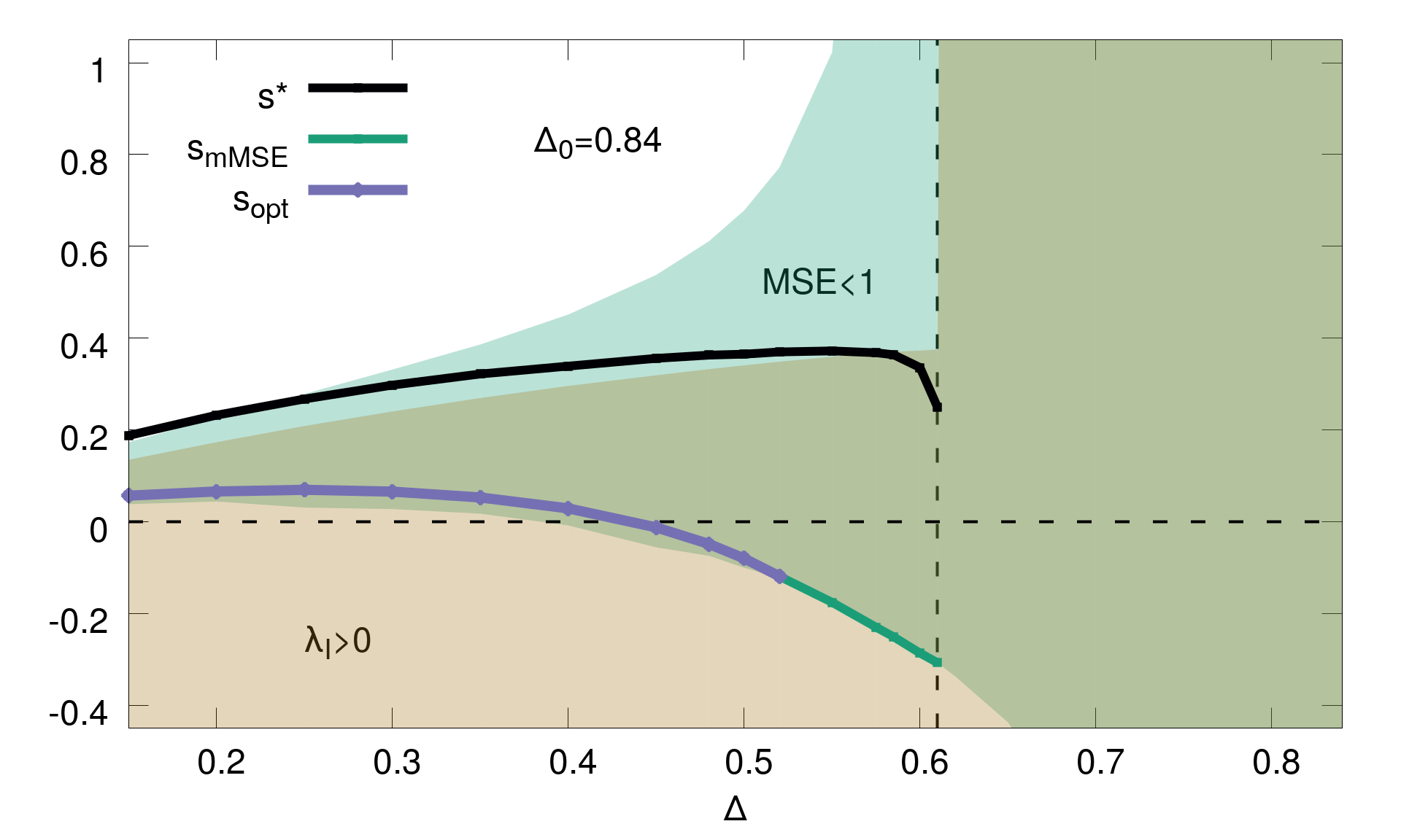
Figure 9: The values of $s_{\rm opt}$ (for which the optimal error is achieved), $s_{\rm mMSE}$ (for which a minimum errors is achieved), and the equilibrium values $s^{*}$ as obtained by solving the 1RSB-SE Eqs. (75)-(78) for the planted SK model with $\Delta_{0}=0.84$. The vertical dashed line is where the RS solution becomes unstable. The light orange and light green regions define the part of the plane where $\lambda_{\text{I}}>0$ and $\text{MSE}<1$, respectively. The common area is dark green. Outside of the $\text{MSE}<1$ region, the solution is such that $\text{MSE}>1$ for larger $s$ and $\text{MSE}=1$ (trivial solution $M=Q=0$) for smaller $s$.

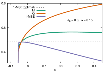
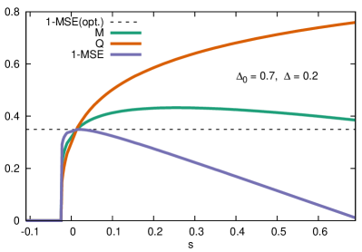
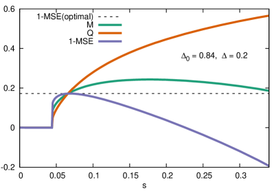
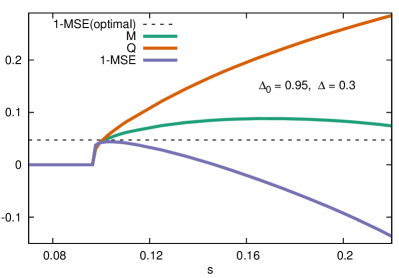
Figure 10: The values of $M$, $Q$ and $1-\text{MSE}=Q-2M$ as obtained by solving the 1RSB-SE Eqs. (75)-(78) for the planted SK model with $\Delta_{0}=0.6,\Delta=0.15$ (top left), $\Delta_{0}=0.7,\Delta=0.2$ (top right), $\Delta_{0}=0.84,\Delta=0.2$ (bottom left), $\Delta_{0}=0.95,\Delta=0.3$ (bottom right) as a function of the Parisi parameter $s$. Note that all these points lie in the RS instability region, cf. Fig. 1. We show the value of MSE obtained by AMP on the Nishimori line as a dashed black line. In all the cases shown, the MSE is minimum when the Nishimori condition $M=Q>0$ is restored: in this point the MSE is equal to the optimal one. The value of $s$ in which the Nishimori condition is satisfied is: $s=-0.0370$ (top left), $s=0.0127$ (top right), $s=0.0658$ (bottom left), $s=0.0994$ (bottom right).

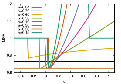
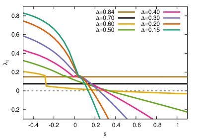
Figure 12: MSE, and the eigenvalue $\lambda_{\text{I}}$ Eq. (94) evaluated from the solution of 1RSB-SE Eqs. (75)-(78) for the planted SK model with $\Delta_{0}=0.84$ varying $s$ for several values of $\Delta$. In this case the RS instability arrives at $\Delta=0.622$.

We denote by $s_{\rm mMSE}$ the value of the Parisi parameter that minimizes the MSE. Quite remarkably, we see in Fig. 8 that for some cases the Bayes-optimal MSE is reached also when $\Delta\neq\Delta_{0}$ for a particular value of the Parisi parameter that we denote $s_{\rm opt}$. This is also seen in Fig. 12 left panel where the MSE is plotted as a function of $s$ for a variety of values of $\Delta$. Moreover, we remark and illustrate in Fig. 9 that the value of the Parisi parameter $s_{\rm mMSE}$ that minimizes the MSE, and $s_{\rm opt}$ for which the Bayes optimal error is reached, are unrelated to the equilibrium value $s^{*}$. Note that, somehow counter-intuitively, very closely under the RS instability the optimality condition $M=Q$ cannot typically be achieved for any value of $s$ (see, e.g., the yellow curve corresponding to $\Delta=0.6$ in Fig. 12): in this case the 1RSB solution depends weakly on $s$ and one explores only a narrow interval in $M$ and $Q$ (that may not include the case $M=Q>0$) before jumping to the trivial solution $M=Q=0$.

In Fig. 9 we show the $s_{\text{opt}}$, and the value $s_{\text{mMSE}}$ for which the MSE is minimum at given $\Delta$ (when $s_{\text{opt}}$ exists the two are equal) and the region where $\text{MSE}<1$ for the SK model with $\Delta_{0}=0.84$. Near the RS instability the MSE depends weakly on $s$ and the $s_{\text{opt}}$ does not exist: in this case the minimum MSE is obtain for the minimum $s$ for which the solution is not trivial (green line). In the same figure we also plot the value of $s^{*}$ that extremizes the Bethe free energy of the model: it is well distinct from $s_{\text{opt}}$.

To clarify the origin of the above observation that Bayes-optimal error can be restored for $s_{\rm opt}$ we remind that in Sec. II.3 we noticed that the inference can be optimal out of the Nishimori line. More precisely, we have put forward a hypothesis that the estimation is optimal every time the Nishimori condition $M=Q>0$ is restored. We showed one example in Fig. 4: introducing a nonzero density of zeros in the prior distribution, it is possible to obtain optimal estimation in the SK model using AMP out of Nishimori. The ASP algorithm naturally introduces a free parameter in the form of the Parisi parameter $s$, cf. Eq. (39). In Fig. 10 we illustrate that minimization of the MSE as a function of $s$ is again related to restoration of the Nishimori condition $M(s)=Q(s)>0$.

This can also be seen analytically by computing the derivative of the MSE with respect to the parameter $s$ at the fixed-point of 1RSB-SE. In the replica theory notation MPV87 ; SD84 we can express this derivative, cf. Appendix B, as

$$\frac{\partial\text{MSE}}{\partial s} =-2\int dh\,\frac{\partial f_{\text{I}}(s,h)}{\partial s}\,D(s,h)$$ (88)

while

$$M-Q=\int dh\,f_{\text{I}}(s,h)\,D(s,h)\,,$$ (89)

with

$$D(s,h)={\mathbb{E}}_{x^{(0)}}\left[\left(f_{\text{I}}^{\prime\prime}(s,h)+f_{\text{I}}^{\prime}(s,h)\frac{T}{\hat{Q}}+x^{(0)}\frac{T}{\hat{Q}}\right)\frac{1}{\sqrt{2\pi(-\hat{Q})}}\exp\left(\frac{T^{2}}{2\hat{Q}}\right)\right]\,,$$ (90)

$\hat{Q}=-\Delta_{0}Q/\Delta^{2}$ and

$$f_{\text{I}}(s,h) =\frac{1}{s}\log{\mathbb{E}}_{W}\left[e^{sf_{\text{II}}(h-\sqrt{V^{(0)}}W)}\right]\,, f_{\text{II}}(h) =\log\,{\mathbb{E}}_{x}\left[\exp\left(-\frac{V^{(1)}}{2}x^{2}+hx\right)\right]\,.$$ (91)

So, if there exists a value of $s$ such that $D(s,h)$ is zero for all $h$, we have that for such value $M=Q$ and MSE is extremized. This is exactly what we observe: at the solution where MSE is minimum the function $D(s,h)$ is zero for all $h$ (and so $M=Q>0$). In this sense we could define the optimal $s_{\rm opt}$ as the value for which at the fixed-point of 1RSB-SE it happens that (if exists)

$$D(s_{\text{opt}},h)={\mathbb{E}}_{x^{(0)}}\left[\left(f_{\text{I}}^{\prime\prime}(s_{\text{opt}},h)+f_{\text{I}}^{\prime}(s_{\text{opt}},h)\frac{T}{\hat{Q}}+x^{(0)}\frac{T}{\hat{Q}}\right)\frac{1}{\sqrt{2\pi(-\hat{Q})}}\exp\left(\frac{T^{2}}{2\hat{Q}}\right)\right]\equiv 0\,.$$ (92)

It seems to us that there should be a deeper theoretical reason behind the observation that the restoration of the Nishimori condition leads to the optimal estimation error. We have not found it and let this question for future work.

III.3.2 Point-wise convergence of ASP

The inclusion of a 1RSB structure into the ASP algorithm extends the region of parameters in which the algorithm converges point-wise with respect to AMP. Note that the range of parameters for which AMP does not converge point-wise corresponds exactly to the range of parameters for which the large iteration time behavior of ASP depends on the Parisi parameter $s$, see Fig. 8, where below the vertical line is exactly where the replicon eigenvalue eq. (35) becomes negative.

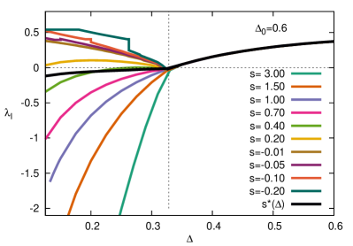
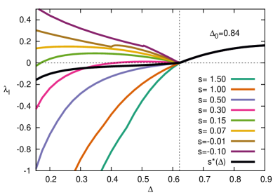
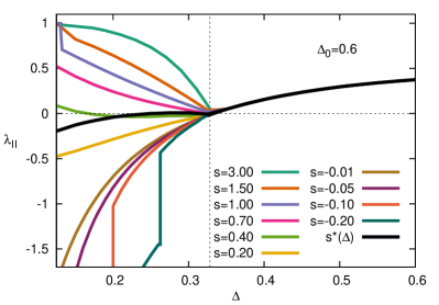
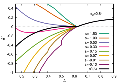
Figure 11: The stability parameters (94-95) as obtained by solving the 1RSB SE Eqs. (75)-(78) for the planted SK model with $\Delta_{0}=0.6$ (left) and $\Delta_{0}=0.84$ (right) varying $\Delta$ and for several $s$. For large $\Delta$ (on the right of the vertical line) the RS solution is stable and ASP converges to the same solution for any $s$. For small $\Delta$ (on the left of the vertical line) the RS solution is unstable, AMP stops converging point-wise and ASP converges if and only if $\lambda_{\text{I}}$ is positive. We plot also the values of $\lambda_{\text{I}}$,$\lambda_{\text{II}}$ obtained by ASP when $s$ is fixed to the equilibrium value $s^{*}(\Delta)$.

ASP converges point-wise in a larger region that AMP, at least for some value of $s$. The analysis of the point-wise convergence of single instances is obtained looking at the Hessian eigenvalues of ASP equations. Again, this can be readily derived by simply repeating the reasoning we used for AMP in section II.2 to reach Eq. (35), using this time ASP Eqs. (84)-(87), instead of the AMP ones Eqs. (28)-(31). This leads to a perturbation growing as $(\Delta_{0}/\Delta^{2}){\mathbb{E}}_{B}\eta^{\prime}(B)$. Leading to the condition

$$\lambda_{\rm ASP}=1-\frac{\Delta_{0}}{\Delta^{2}}\mathbb{E}_{x^{(0)},T}\left[\left(\frac{1}{s}\frac{\partial^{2}f_{\rm in}(T,V_{1},V_{0})}{\partial T^{2}}\right)^{2}\right]\,.$$ (93)

Interestingly, this corresponds to a well known quantity in the replica theory MPV87 ; SD84 , that appears in the stability of the 1RSB solution against further breaking of replica symmetry. In in this case (see Appendix A) two kind of instabilities are often discussed MonRic03 ; MonParRic04 ; KrzPagWei04 ; MerMezZec05 and the two eigenvalues that express the 1RSB stability can be written as

$$\lambda_{\text{I}} =1-\frac{\Delta_{0}}{\Delta^{2}}\int_{-\infty}^{\infty}\mathrm{d}hP_{\text{I}}(h)\left(f_{\text{I}}^{\prime\prime}(s,h)\right)^{2}\,,$$ (94)

$$\lambda_{\text{II}} =1-\frac{\Delta_{0}}{\Delta^{2}}\int_{-\infty}^{\infty}\mathrm{d}hP_{\text{II}}(s,h)\left(f_{\text{II}}^{\prime\prime}(h)\right)^{2}\>.$$ (95)

where

$$f_{\text{II}}(h) =\log\,{\mathbb{E}}_{x}\left[\exp\left(-\frac{V^{(1)}}{2}x^{2}+hx\right)\right]$$ (96)

$$f_{\text{I}}(s,h) =\frac{1}{s}\log{\mathbb{E}}_{W}\left[e^{sf_{\text{II}}(h-\sqrt{V^{(0)}}W)}\right]$$ (97)

$$P_{\text{I}}\left(h\right) =\frac{\Delta}{\sqrt{2\pi\Delta_{0}Q}}{\mathbb{E}}_{x^{(0)}}\left[\exp\left(-\frac{\Delta^{2}}{2\Delta_{0}Q}\left(\frac{M}{\Delta}x^{(0)}+h\right)^{2}\right)\right]$$ (98)

$$P_{\text{II}}(s,h) =e^{sf_{\text{II}}(h)}\,{\mathbb{E}}_{W}\left[P_{\text{I}}(h-\sqrt{V^{(0)}}W)\,e^{-sf_{\text{I}}(s,h-\sqrt{V^{(0)}}W)}\right]$$ (99)

with $V^{(1)},V^{(0)}$ given by Eqs. (73)-(74) and $x$, $x^{(0)}$ and $W$ being random variables distributed according $P(x)$, $P^{(0)}(x)$ and a standard Gaussian distribution, respectively.

A change of variable, as in Appendix A, shows that $\lambda_{\rm ASP}=\lambda_{\text{I}}$: the convergence of the ASP algorithm is determined by the first-type instability towards further replica symmetry breaking, just as it is for Survey Propagation MonParRic04 ; KrzPagWei04 ; MerMezZec05 .

In the region of RS stability $\Delta^{(0)}=V^{(0)}=0$ and the two eigenvalues are equal and coincide with the RS replicon eigenvalue in Eq. (35). To understand the meaning of these two eigenvalues consider that the 1RSB structure consists of equivalent metastable states whose distance from each other is given by $Q$. There are then two ways in which a further hierarchical level of RSB states can appear: the 1RSB states can aggregate in a way to establish a new scale of distance between states (type I instability, associated to negative $\lambda_{\text{I}}$), or each metastable state can split into a hierarchy of new states (type II instability, associated to negative $\lambda_{\text{II}}$).

Let us discuss the behavior of the eigenvalues as we move away from the Nishimori line. To be concrete, we keep referring to the case of the planted SK model Eq. (8), cf. Fig. 11. In the RS stability region, the two eigenvalues are equal and positive. At the boundary of the RS stability region, the eigenvalues become marginal and the replica symmetry gets broken: beyond this line the solution of the 1RSB-SE depends on $s$ and so do $\lambda_{\text{I}}$ and $\lambda_{\text{II}}$. For the low-rank matrix estimation problem, the transition is towards a full replica symmetry broken (FRSB) state MPV87 , so that the 1RSB states are always unstable and at least one among $\lambda_{\text{I}}$ and $\lambda_{\text{II}}$ is negative beyond the RS instability line. Nevertheless, unlike the RS algorithm laid out by AMP, in ASP there is a scale of distance among state - tuned via the $s$ parameter - so that the algorithm can converge point-wise also when the inner structure of the states is more complicated than 1RSB. In Fig. 11 we show the value of $\lambda_{\text{I}}$ and $\lambda_{\text{II}}$ crossing the RS stability line for several values of $s$. We see $\lambda_{\text{I}}$ is positive for $s$ sufficiently small, indicating that ASP converges point-wise for such values also in the RSB region (cf. Fig. 6).

III.3.3 Results on single instances of ASP

So far we mostly concentrated on results of the state evolution of the ASP algorithm. We now show that these results are indeed describing the behaviour of the ASP algorithm run on large but finite-size instances.

In Fig. 7 we compared how the error evolves as a function of the iteration time for the state evolution an the ASP algorithm of several instances of two different system sizes ($N=2000$ and $N=64000$). We see that for the large system size the finite size effects are small enough and the agreement with the theory is rather good for each of the runs.

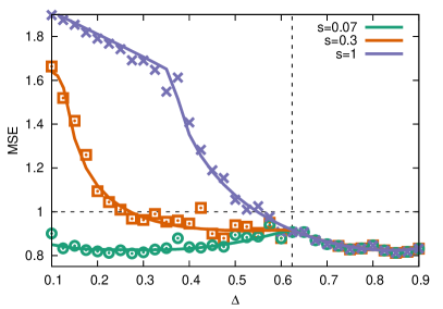
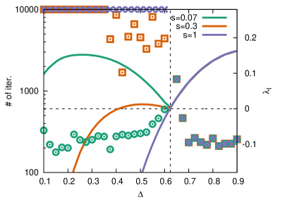
Figure 13: MSE and convergence time of ASP for $N=50000$ with $s=0.07$, $s=0.3$ and $s=1$ (equivalent to AMP) for the SK model with $\Delta_{0}=0.84$ varying $\Delta$. Each point is an average over 3 instances of the problem. The iterations are stopped when the average change of a variable in a single iteration of ASP is less than $10^{-8}$ or at $10^{4}$ iterations if convergence is not reached. The continuous line are the values of MSE (left) and of $\lambda_{\text{I}}$ (right) obtained with the 1RSB-SE Eqs. (75)-(78).

In Fig. 13 we report the result of ASP for size $N=5\times 10^{4}$ and $s=0.07$, $0.3$, $1$ in the same situation of the right column of Figs. 8 and 11. We see that in the RS region the fixed-point is the same for all $s$ while in the RSB region the result depends strongly on $s$. Note that for $s=0.07$ the MSE is less than 1 for any $\Delta$ in all the instances. The convergence time is increasing for any $s$ at the RS stability – where $\lambda_{\text{I}}=0$ – but the algorithm keeps converging point-wise for $s=0.07$ even at low $\Delta$, as predicted by the positivity of $\lambda_{\text{I}}$ from 1RSB-SE at $s=0.07$. In general, we see as for this size the trend predicted by SE is visible in the MSE obtained by ASP.

Finally, in Figs. 14 we show the heat-maps of the MSE (left panels) and convergence times (right panels) as obtained by the ASP algorithm run on single instances of $N=5000$ variables and, respectively, $s=0.5$, $s=0.1$ and $s=0.02$. We use the same color-map as Fig. 2, to enhance the difference w.r.t. AMP. On this scale, ASP with $s=0.5$ is very similar to AMP, but for $s=0.1$ and $s=0.02$ the difference becomes evident. In particular, the $\text{MSE}<1$ and convergence region extend to lower values of $\Delta$ including sections of the RSB region, cf. Fig. 1. It is visible that the convergence time increases at the RS instability boundary, where $\lambda_{\text{I}}=0$, but then for $s=0.1$ and $s=0.02$ the convergence time goes down again beyond the RS instability. Note that also the region of convergence to the trivial point $Q=M=0$ is extended, so that for very small $s$ the ASP algorithm convergences point-wise to either the trivial or to nontrivial fixed-point in most of the phase diagram.

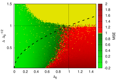
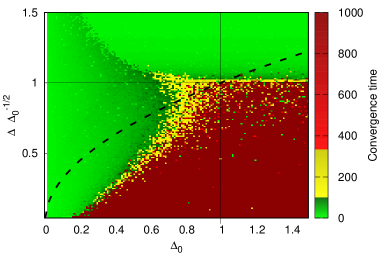
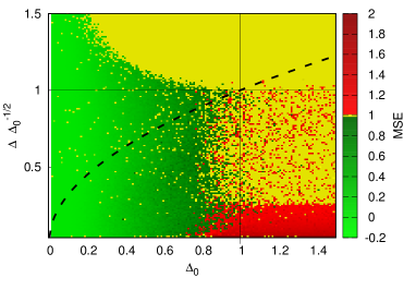
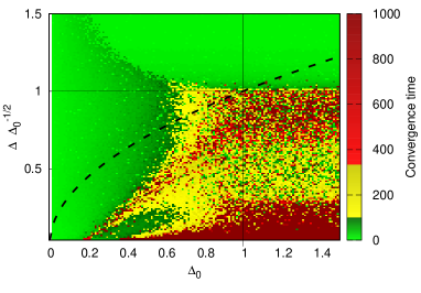
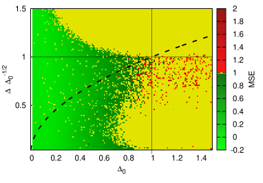
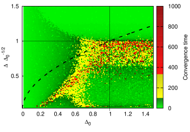
Figure 14: Heat-map of the MSE (left) and convergence time (right) obtained running ASP for $s=0.5$ (top), $s=0.1$ (middle) and $s=0.02$ (bottom) for size $N=5000$ for the planted SK model. The dashed line is the Nishimori line $\Delta=\Delta_{0}$. The iterations are stopped after 1000 iterations or as soon as the average change of a variable in a single iteration of ASP is less than $10^{-8}$.

IV Conclusions and open questions

In this paper we introduced the approximate survey propagation (ASP) algorithm for the class of low-rank matrix estimation problems. We derived the state evolution describing the large size behavior of the algorithm, finding that the fixed-points of the state evolution of ASP reproduce the one-step replica symmetric fixed-point equations well-known in physics of disordered systems.

This leads to a new algorithmic interpretation of the replica method where the self-consistent equations actually describe the behavior of an iterative algorithm: AMP in the replica symmetric case, and ASP when the replica symmetry is broken (just as BP and SP corresponds to the same situation on sparse graphs).

We characterize the performance of ASP in terms of convergence and mean-squared error as a function of the free Parisi parameter $s$. In particular, we reported the results of the algorithm for the analysis of the planted Sherrington-Kirkpatrick model. Notably we found that when there is a model mismatch between the true generative model and the inference model, the performance of AMP rapidly degrades both in terms of MSE and of convergence. Using ASP for a suitably chosen value of $s$ we observed we can always restore convergence and improve the estimation error.

Among other results, our analysis leads us to a striking hypothesis that whenever $s$ (or other parameters) can be set in such a way that the Nishimori condition $M=Q>0$ is restored, then the algorithm is able to reach mean-squared error as low as the Bayes-optimal error obtained on the Nishimori line, i.e. when the model and its parameters are known and matched in the inference procedure. Another hypothesis to which we have not find a counter-example in the present model is whether the Nishimori condition $M=Q$ implies convergence of the ASP algorithm. Whenever $M=Q$ we always observed that ASP converges point-wise to a fixed-point with minimal MSE even if the generative model and the inference model are highly mismatched. Unveiling the physical origin and range of validity of these properties is an interesting direction for future work.

Another direction for future work is an algorithmic procedure able to select values of the Parisi parameter $s$ that lead to low estimation errors. In this paper we remark that the standard methods based on expectation maximization or choice of the equilibrium value of $s^{*}$ are sub-optimal.

Finally, we mention that the derivation we have done here to obtain the ASP algorithm can be easily generalized along the same lines to an arbitrary number of replica symmetry breaking levels. While to formally derive such algorithm is in principle straightforward, it is not obvious what are the algorithmic consequences in terms of estimation error and convergence in comparison to AMP and ASP. This is also left for future work.

Appendix A The 1RSB-SE: equivalence with the 1RSB replica calculation

We want to show the 1RSB state evolution coincides with the replica result. Here we will not verify that all the equations coincides, but we will limit ourselves to show that Eq. (70) for $M$ coincides with the equation for the magnetization of the replica result. In a 1RSB ansatz, the overlap matrix has the form of a block matrix in which the inner block of size $s$ has values $q_{1}$ while outside of the block the value is in principle different and indicated with $q_{0}$ MPV87 . The diagonal value of the overlap matrix is $q_{d}$. The free energy of the system takes the form

$$F_{\text{1RSB}}= \frac{1}{4\Delta}\left\{\frac{\Delta-\Delta_{0}}{\Delta}q_{d}^{2}-2M^{2}+\frac{\Delta_{0}}{\Delta}\left[sq_{0}^{2}+(1-s)q_{1}^{2}\right]\right\}+\int\mathrm{d}h\,P_{\text{I}}(h)\,f_{\text{I}}(s,h)$$ (100)

where the functions $P_{\text{I}}(h)$ and $f_{\text{I}}(s,h)$ are equal to the expressions in Eqs. (96)-(99) provided that

$$\Delta^{(0)}=q_{1}-q_{0}\,, Q=q_{0}\,, \Delta^{(1)}=q_{d}-q_{1}\,.$$ (101)

The value of the magnetization, namely the overlap of the ground truth with the inferred signal, that extremizes the free energy satisfies the following equation

$$M= \int dh\,\Delta\,\frac{\partial P_{\text{I}}(h)}{\partial M}\,f_{\text{I}}(s,h)=\int dh\,\int Dx^{(0)}\Delta\,\frac{\partial p_{\text{I}}(h,x^{(0)})}{\partial M}\,f_{\text{I}}(s,h)=$$ (102)

$$= \int dh\,\int Dx^{(0)}\,x^{(0)}\,\frac{\partial p_{\text{I}}(h,x^{(0)})}{\partial h}\,f_{\text{I}}(s,h)=-\int dh\,\int Dx^{(0)}\,x^{(0)}\,p_{\text{I}}(h,x^{(0)})\,f^{\prime}_{\text{I}}(s,h)$$ (103)

where $p_{\text{I}}(h,x^{(0)})$ is defined such that $P_{\text{I}}(h)={\mathbb{E}}_{x^{(0)}}\left[p_{\text{I}}(h,x^{(0)})\right]$ and $Dx^{(0)}\equiv dx^{(0)}P_{0}(x^{(0)})$. Now rescaling the integration variable $h$ as

$$h=-\frac{\sqrt{\Delta_{0}Q}}{\Delta}W-\frac{M}{\Delta}x^{(0)}$$ (104)

where $W$ is a standard Gaussian random variable, we obtain the 1RSB-SE Eq. (75). The equations for $q_{0}$, $q_{d}$ and $q_{1}$ can be obtained on the same lines.

Appendix B Derivative of MSE wrt $s$

In replica theory notation, cf. Appendix A, the equations for $M$ and $Q$ can be written as

$$M =\int\mathrm{d}h\,\Delta\left[\frac{\partial}{\partial M}P_{\text{I}}(h)\right]f_{\text{I}}(s,h)\,, Q =\int\mathrm{d}hP_{\text{I}}(h)\left(f_{\text{I}}^{\prime}(s,h)\right)^{2}\,,$$ (105)

where the functions $P_{\text{I}}(h)$ and $f_{\text{I}}(s,h)$ are given in Eqs. (96)-(99). So that we have

$$M-Q=\int dh\,f_{\text{I}}(s,h)\left[\Delta\frac{\partial P_{\text{I}}(h)}{\partial M}+\frac{\partial}{\partial h}\left(P_{\text{I}}(h)\,f_{\text{I}}^{\prime}(s,h)\right)\right]\equiv\int dh\,f_{\text{I}}(s,h)\,D(s,h)\,,$$ (106)

Therefore, the derivative of the MSE wrt $s$ is given by

$$\frac{\partial\text{MSE}}{\partial s} =M-Q-{\mathbb{E}}_{x^{(0)},W}\left[\left(x^{(0)}-\frac{1}{s}\frac{\partial f_{in}}{\partial T}\right)\,\frac{\partial}{\partial s}\frac{\partial f_{in}}{\partial T}\right]=$$ (107)

$$=-2\int dh\,\frac{\partial f_{\text{I}}(s,h)}{\partial s}\left[\Delta\frac{\partial P_{\text{I}}(h)}{\partial M}+\frac{\partial}{\partial h}\left(P_{\text{I}}(h)\,f_{\text{I}}^{\prime}(s,h)\right)\right]=$$ (108)

$$=-2\int dh\,\frac{\partial f_{\text{I}}(s,h)}{\partial s}\,D(s,h)\,.$$ (109)

Replacing the explicit expression of $P_{\text{I}}(h)$ in the previous definition of $D(s,h)$, we obtain Eq. (90).

Alternately, defining $p_{\text{I}}(h,x^{(0)})$ such that $P_{\text{I}}(h)={\mathbb{E}}_{x^{(0)}}\left[p_{\text{I}}(h,x^{(0)})\right]$, we can express the two quantities as

$$M-Q =-\int dh\,f^{\prime}_{\text{I}}(s,h)\,\int Dx^{(0)}\,p_{\text{I}}(h,x^{(0)})\,\left[x^{(0)}+f^{\prime}_{\text{I}}(s,h)\right]\,,$$ (110)

$$\frac{\partial\text{MSE}}{\partial s} =-2\int dh\,\frac{\partial f^{\prime}_{\text{I}}(s,h)}{\partial s}\,\int Dx^{(0)}\,p_{\text{I}}(h,x^{(0)})\,\left[x^{(0)}+f^{\prime}_{\text{I}}(s,h)\right]\,.$$ (111)

where $Dx^{(0)}\equiv dx^{(0)}P_{0}(x^{(0)})$. The condition $D(s,h)=0$, that implies $M=Q$ and the extremization of the MSE, is then also equivalent to

$$\int Dx^{(0)}\,p_{\text{I}}(h,x^{(0)})\,x^{(0)}=-P_{\text{I}}(h)\,f^{\prime}_{\text{I}}(s,h) \rightarrow f^{\prime}_{\text{I}}(s,h)=-\langle x^{(0)}\rangle_{p_{I}}$$ (112)

where the average is over the distribution $p_{\text{I}}(h,x^{(0)})/P_{\text{I}}(h)$ and the condition must hold for any $h$.

References

- (1) R. M. Neal, “Markov chain sampling methods for dirichlet process mixture models,” Journal of computational and graphical statistics, vol. 9, no. 2, pp. 249–265, 2000.
- (2) M. J. Wainwright, M. I. Jordan, et al., “Graphical models, exponential families, and variational inference,” Foundations and Trends® in Machine Learning, vol. 1, no. 1–2, pp. 1–305, 2008.
- (3) L. Bottou, “Large-scale machine learning with stochastic gradient descent,” in Proceedings of COMPSTAT’2010, pp. 177–186, Springer, 2010.
- (4) D. J. Thouless, P. W. Anderson, and R. G. Palmer, “Solution of ’solvable model of a spin glass’,” Philosophical Magazine, vol. 35, no. 3, pp. 593–601, 1977.
- (5) D. L. Donoho, A. Maleki, and A. Montanari, “Message-passing algorithms for compressed sensing,” Proc. Natl. Acad. Sci., vol. 106, no. 45, pp. 18914–18919, 2009.
- (6) E. Bolthausen, “An iterative construction of solutions of the tap equations for the sherrington–kirkpatrick model,” Communications in Mathematical Physics, vol. 325, no. 1, pp. 333–366, 2014.
- (7) M. Bayati and A. Montanari, “The dynamics of message passing on dense graphs, with applications to compressed sensing,” IEEE Transactions on Information Theory, vol. 57, no. 2, pp. 764–785, 2011.
- (8) A. Javanmard and A. Montanari, “State evolution for general approximate message passing algorithms, with applications to spatial coupling,” Information and Inference, p. iat004, 2013.
- (9) M. Mézard, G. Parisi, and M. A. Virasoro, Spin glass theory and beyond. Singapore: World Scientific, 1987.
- (10) D. Donoho and A. Montanari, “High dimensional robust m-estimation: Asymptotic variance via approximate message passing,” Probability Theory and Related Fields, vol. 166, no. 3-4, pp. 935–969, 2016.
- (11) M. Advani and S. Ganguli, “Statistical mechanics of optimal convex inference in high dimensions,” Physical Review X, vol. 6, no. 3, p. 031034, 2016.
- (12) L. Zdeborová and F. Krzakala, “Statistical physics of inference: Thresholds and algorithms,” Advances in Physics, vol. 65, pp. 453–552, 2016.
- (13) T. Lesieur, F. Krzakala, and L. Zdeborová, “Constrained low-rank matrix estimation: phase transitions, approximate message passing and applications,” Journal of Statistical Mechanics: Theory and Experiment, vol. 2017, no. 7, p. 073403, 2017.
- (14) H. Nishimori, Statistical Physics of Spin Glasses and Information Processing: An Introduction. Oxford, UK: Oxford University Press, 2001.
- (15) D. Sherrington and S. Kirkpatrick, “Solvable model of a spin-glass,” Phys. Rev. Lett., vol. 35, pp. 1792–1796, 1975.
- (16) M. Mézard, G. Parisi, and R. Zecchina, “Analytic and algorithmic solution of random satisfiability problems,” Science, vol. 297, no. 5582, pp. 812–815, 2002.
- (17) A. Braunstein, M. Mézard, and R. Zecchina, “Survey propagation: An algorithm for satisfiability,” Random Structures & Algorithms, vol. 27, no. 2, pp. 201–226, 2005.
- (18) M. Yasuda, Y. Kabashima, and K. Tanaka, “Replica plefka expansion of ising systems,” Journal of Statistical Mechanics: Theory and Experiment, vol. 2012, no. 04, p. P04002, 2012.
- (19) J. De Almeida and D. J. Thouless, “Stability of the sherrington-kirkpatrick solution of a spin glass model,” Journal of Physics A: Mathematical and General, vol. 11, no. 5, p. 983, 1978.
- (20) J. Wright, A. Ganesh, S. Rao, Y. Peng, and Y. Ma, “Robust principal component analysis: Exact recovery of corrupted low-rank matrices via convex optimization,” in Advances in neural information processing systems, pp. 2080–2088, 2009.
- (21) E. J. Candès, X. Li, Y. Ma, and J. Wright, “Robust principal component analysis?,” Journal of the ACM (JACM), vol. 58, no. 3, p. 11, 2011.
- (22) E. J. Candès and B. Recht, “Exact matrix completion via convex optimization,” Foundations of Computational mathematics, vol. 9, no. 6, p. 717, 2009.
- (23) T. Lesieur, F. Krzakala, and L. Zdeborová, “Mmse of probabilistic low-rank matrix estimation: Universality with respect to the output channel,” in 53rd Annual Allerton Conference on Communication, Control, and Computing, pp. 680–687, IEEE, 2015.
- (24) F. Krzakala, J. Xu, and L. Zdeborová, “Mutual information in rank-one matrix estimation,” in Information Theory Workshop (ITW), 2016 IEEE, pp. 71–75, IEEE, 2016.
- (25) L. Zdeborová and F. Krzakala, “Generalization of the cavity method for adiabatic evolution of gibbs states,” Physical Review B, vol. 81, no. 22, p. 224205, 2010.
- (26) G. Parisi, “Infinite number of order parameters for spin-glasses,” Physical Review Letters, vol. 43, no. 23, p. 1754, 1979.
- (27) S. Rangan and A. K. Fletcher, “Iterative estimation of constrained rank-one matrices in noise,” in IEEE International Symposium on Information Theory Proceedings (ISIT), pp. 1246–1250, IEEE, 2012.
- (28) R. Matsushita and T. Tanaka, “Low-rank matrix reconstruction and clustering via approximate message passing,” in Advances in Neural Information Processing Systems 26 (C. Burges, L. Bottou, M. Welling, Z. Ghahramani, and K. Weinberger, eds.), pp. 917–925, Curran Associates, Inc., 2013.
- (29) Y. Deshpande and A. Montanari, “Information-theoretically optimal sparse PCA,” in IEEE International Symposium on Information Theory (ISIT), pp. 2197–2201, IEEE, 2014.
- (30) T. Lesieur, F. Krzakala, and L. Zdeborová, “Phase transitions in sparse PCA,” in IEEE International Symposium on Information Theory Proceedings (ISIT), pp. 1635–1639, 2015.
- (31) Y. Deshpande, E. Abbe, and A. Montanari, “Asymptotic mutual information for the binary stochastic block model,” in 2016 IEEE International Symposium on Information Theory (ISIT), pp. 185–189, July 2016.
- (32) J. Barbier, M. Dia, N. Macris, F. Krzakala, T. Lesieur, and L. Zdeborová, “Mutual information for symmetric rank-one matrix estimation: A proof of the replica formula,” in Advances In Neural Information Processing Systems, pp. 424–432, 2016.
- (33) M. Lelarge and L. Miolane, “Fundamental limits of symmetric low-rank matrix estimation,” arXiv:1611.03888 [math.PR], 2016.
- (34) J. Barbier and N. Macris, “The stochastic interpolation method: A simple scheme to prove replica formulas in bayesian inference,” arXiv preprint arXiv:1705.02780, 2017.
- (35) A. E. Alaoui and F. Krzakala, “Asymptotic mutual information for the binary stochastic block modelestimation in the spiked wigner model: A short proof of the replica formula,” in 2018 IEEE International Symposium on Information Theory (ISIT), 2018.
- (36) S. B. Korada and N. Macris, “Exact solution of the gauge symmetric p-spin glass model on a complete graph,” Journal of Statistical Physics, vol. 136, no. 2, pp. 205–230, 2009.
- (37) M. Mézard, “Mean-field message-passing equations in the hopfield model and its generalizations,” Phys. Rev. E, vol. 95, p. 022117, Feb 2017.
- (38) M. Gabrié, E. W. Tramel, and F. Krzakala, “Training restricted boltzmann machine via the thouless-anderson-palmer free energy,” in Advances in Neural Information Processing Systems 28 (C. Cortes, N. D. Lawrence, D. D. Lee, M. Sugiyama, and R. Garnett, eds.), pp. 640–648, Curran Associates, Inc., 2015.
- (39) E. W. Tramel, A. Manoel, F. Caltagirone, M. Gabrié, and F. Krzakala, “Inferring sparsity: Compressed sensing using generalized restricted boltzmann machines,” in Information Theory Workshop (ITW), 2016 IEEE, pp. 265–269, 2016.
- (40) J. Tubiana and R. Monasson, “Emergence of compositional representations in restricted boltzmann machines,” Phys. Rev. Lett., vol. 118, p. 138301, Mar 2017.
- (41) J. S. Yedidia, W. T. Freeman, and Y. Weiss, “Understanding belief propagation and its generalizations,” Exploring artificial intelligence in the new millennium, vol. 8, pp. 236–239, 2003.
- (42) T. Plefka, “Convergence condition of the tap equation for the infinite-ranged ising spin glass model,” Journal of Physics A: Mathematical and general, vol. 15, no. 6, p. 1971, 1982.
- (43) A. Georges and J. S. Yedidia, “How to expand around mean-field theory using high-temperature expansions,” Journal of Physics A: Mathematical and General, vol. 24, no. 9, p. 2173, 1991.
- (44) S. Rangan, P. Schniter, E. Riegler, A. K. Fletcher, and V. Cevher, “Fixed points of generalized approximate message passing with arbitrary matrices,” IEEE Transactions on Information Theory, vol. 62, no. 12, pp. 7464–7474, 2016.
- (45) J. Vila, P. Schniter, S. Rangan, F. Krzakala, and L. Zdeborová, “Adaptive damping and mean removal for the generalized approximate message passing algorithm,” in IEEE International Conference on Acoustics, Speech and Signal Processing (ICASSP), pp. 2021–2025, IEEE, 2015.
- (46) H. Nishimori and D. Sherrington, “Absence of replica symmetry breaking in a region of the phase diagram of the ising spin glass,” in AIP Conference Proceedings, vol. 553, pp. 67–72, AIP, 2001.
- (47) M. Mézard and G. Parisi, “The bethe lattice spin glass revisited,” The European Physical Journal B-Condensed Matter and Complex Systems, vol. 20, no. 2, pp. 217–233, 2001.
- (48) M. Mézard and G. Parisi, “The cavity method at zero temperature,” Journal of Statistical Physics, vol. 111, no. 1-2, pp. 1–34, 2003.
- (49) R. Monasson, “Structural glass transition and the entropy of the metastable states,” Phys. Rev. Lett., vol. 75, pp. 2847–2850, Oct 1995.
- (50) P. Charbonneau, J. Kurchan, G. Parisi, P. Urbani, and F. Zamponi, “Glass and jamming transitions: From exact results to finite-dimensional descriptions,” Annual Review of Condensed Matter Physics, vol. 8, pp. 265–288, 2017.
- (51) P. Charbonneau, J. Kurchan, G. Parisi, P. Urbani, and F. Zamponi, “Fractal free energies in structural glasses,” Nature Communications, vol. 5, p. 3725, 2014.
- (52) P. Charbonneau, J. Kurchan, G. Parisi, P. Urbani, and F. Zamponi, “Exact theory of dense amorphous hard spheres in high dimension. iii. the full replica symmetry breaking solution,” J. Stat. Mech.: Theor. Exp., vol. 2014, no. 10, p. P10009, 2014.
- (53) H.-J. Sommers and W. Dupont, “Distribution of frozen fields in the mean-field theory of spin glasses,” Journal of Physics C: Solid State Physics, vol. 17, no. 32, p. 5785, 1984.
- (54) Montanari, A. and Ricci-Tersenghi, F., “On the nature of the low-temperature phase in discontinuous mean-field spin glasses,” Eur. Phys. J. B, vol. 33, no. 3, pp. 339–346, 2003.
- (55) A. Montanari, G. Parisi, and F. Ricci-Tersenghi, “Instability of one-step replica-symmetry-broken phase in satisfiability problems,” Journal of Physics A: Mathematical and General, vol. 37, no. 6, p. 2073, 2004.
- (56) F. Krzakala, A. Pagnani, and M. Weigt, “Threshold values, stability analysis, and high- asymptotics for the coloring problem on random graphs,” Phys. Rev. E, vol. 70, p. 046705, Oct 2004.
- (57) S. Mertens, M. Mézard, and R. Zecchina, “Threshold values of random k‐sat from the cavity method,” Random Structures & Algorithms, vol. 28, no. 3, pp. 340–373, 2005.