Exchange of optical vortices using an electromagnetically induced transparency based four-wave mixing setup

Abstract

We propose a scheme to exchange optical vortices of slow light using the phenomenon of electromagnetically induced transparency (EIT) in a four-level double-$\Lambda$ atom-light coupling scheme illuminated by a pair of probe fields as well as two control fields of larger intensity. We study the light-matter interaction under the situation where one control field carries an optical vortex, and another control field has no vortex. We show that the orbital angular momentum (OAM) of the vortex control beam can be transferred to a generated probe field through a four-wave mixing (FWM) process and without switching on and off of the control fields. Such a mechanism of OAM transfer is much simpler than in a double-tripod scheme in which the exchange of vortices is possible only when two control fields carry optical vortices of opposite helicity. The losses appearing during such OAM exchange are then calculated. It is found that the one-photon detuning plays an important role in minimizing the losses. An approximate analytical expression is obtained for the optimal one-photon detuning for which the losses are minimum while the intensity of generated probe field is maximum. The influence of phase mismatch on the exchange of optical vortices is also investigated. We show that in presence of phase mismatch the exchange of optical vortices can still be efficient.

I Introduction

With the recent progress in quantum optics and laser physics, a significant attention has been drawn to novel approaches Kawazoe et al. (2003); Jiang et al. (2004) which enable coherent control of interaction between radiation and matter. A promising and flexible technique to manipulating pulse propagation characteristics in atomic structures involves the quantum interference and coherence Fleischhauer et al. (2005, 1992); Harris et al. (1990); Zibrov et al. (1995); Harris (1997); Fleischhauer and Lukin (2000). It turns out that the quantum interference between different excitation channels is the basic mechanism for modifying optical response of the medium to the applied fields, allowing to control the optical properties of the medium. A destructive quantum interference in an absorbing medium can suppress the absorption of the medium. This effect has given the name Electromagnetically induced transparency (EIT) Fleischhauer and Lukin (2000); Harris (1997); Fleischhauer et al. (2005). An EIT medium can be very dispersive resulting in a slowly propagating beam of the electromagnetic radiation. The slow light Sahrai et al. (2004); Ruseckas et al. (2011, 2007); Fleischhauer and Juzeliūnas (2016); Hamedi et al. (2017), forming due to the EIT can greatly enhance the atom-light interaction resulting in a number of distinctive optical phenomena Schmidt and Imamoglu (1996); Sahrai et al. (2005); Harshawardhan and Agarwal (1996); Imamoḡlu et al. (1997); Zhu (1992); Hamedi and Juzeliūnas (2015, 2016).

On the other hand, orbital angular momentum (OAM) of light provides additional possibilities in manipulating the light propagation characteristics L.Allen et al. (1999); Yao and Padgett (2011). The OAM also represents an extra degree of freedom in controlling the slow light Ruseckas et al. (2007, 2011, 2013), which can be exploited in quantum computation and quantum information storage Allen et al. (2003).

Most scenarios considered earlier deals with the three-level $\Lambda$-type level structure in which the incident probe field has a vortex Dutton and Ruostekoski (2004); Pugatch et al. (2007); Wang et al. (2008a, b); Moretti et al. (2009), yet the control beam does not carry OAM. If the control beam carries an OAM, the EIT is destroyed resulting in the absorption losses at the vortex core. This is due to the zero intensity at the core of the vortex beam. To avoid such losses, a four-level atom-light coupling tripod-type configuration Unanyan et al. (1998); N.Gavra et al. (2007); Raczyński et al. (2007); Mazets (2005); Ruseckas et al. (2005); Wang et al. (2004); Petrosyan and Malakyan (2004); Rebić et al. (2004); Paspalakis and Knight (2002) was suggested with an extra control laser beam without an optical vortex Ruseckas et al. (2011). The total intensity of the control lasers is then nonzero at the vortex core of the first control laser thus avoiding the losses. It was shown that the OAM of the control field can be transferred to the probe field in such a medium during switching off and on the control beams Ruseckas et al. (2011). Later a more complex double tripod (DT) scheme of the atom-light coupling with six laser fields was employed to transfer of the vortex between the control and probe beams without switching off and on the control beams Ruseckas et al. (2013). However, the transfer of the optical vortex in the DT scheme takes place only when two control beams carry optical vortices of opposite helicity. In this paper we consider a much simpler four-level double-$\Lambda$ (DL) EIT scheme for the exchange of optical vortices.

The DL atom–light coupling scheme has attracted a great deal of attention due to its important applications in coherent control of pulse propagation characteristics Deng et al. (2005); Kang et al. (2011); Korsunsky and Kosachiov (1999); Li et al. (2006); Chen et al. (a, b); Liu et al. (2004); Huss et al. (2002); Liu et al. (2016); Wang et al. (2006); Raczyński et al. (2004); Huang et al. (2006); Kang et al. (2006); Xu et al. (2013); Wu (2008); Moiseev and Ham (2006); Payne and Deng (2002); Kim et al. (2013); Sahrai et al. (2009); Chong and Soljačić (2008); Shpaisman et al. (2005); Chiu et al. (2014); McCormick et al. (2007); Turnbull et al. (2013); Alaeian and Shahriar . All involved transitions in the DL scheme are excited by laser radiation making a closed-loop phase sensitive coherent coupling scheme. It was shown that an interference of excitation channels in such closed-loop systems results in a strong dependence of the atomic state on the relative phase and the relative amplitudes of the applied fields Korsunsky and Kosachiov (1999). As a result, the response of such a medium may be controlled by the relative phase. Phase control of EIT in DL scheme has been investigated in details both theoretically Chen et al. (a) and experimentally Liu et al. (2016). The EIT as well as light storing have been discussed in the case of two signal pulses propagating in a four-level DL scheme Raczyński et al. (2004). Observation of interference between three-photon and one-photon excitations, and phase control of light attenuation or transmission in a medium of four-level atoms in DL configuration was reported by Kang et al. Kang et al. (2006). Moiseev and Ham have presented the two-color stationary light and quantum wavelength conversion using double quantum coherence in a DL atomic structure Moiseev and Ham (2006). All-optical image switching was demonstrated in a DL system, with optical images generated by two independent laser sources Kim et al. (2013). It has been shown both analytically and numerically that a DL scheme characterized by parametric amplification of cross-coupled probe and four-wave mixing pulses, is an excellent medium for producing both slow and stored light Eilam et al. (2008).

In this paper we employ DL level structure in order to exchange of optical vortices between control and probe fields. It is shown that the OAM of the control field can be transferred from the control field to a generated probe field through a four-wave mixing (FWM) process and without switching on and off of the control fields. We calculate the losses appearing during such vortex exchange and obtain an approximate analytical expression for the optimal one-photon detuning for which the intensity of generated probe beam is maximum and the losses are minimum.

II Theoretical model and formulation

II.1 The double-$\Lambda$ system

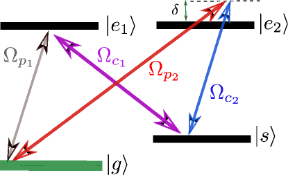
Figure 1: Schematic diagram of the four-level Double-$\Lambda$ (DL) quantum system.

We shall analyze the light-matter interaction in an ensemble of atoms using a four-level double-$\Lambda$ (DL) scheme shown in Fig. 1. The atoms are characterized by two metastable ground states $|g\rangle$ and $|s\rangle$, as well as two excited states $|e_{1}\rangle$ and $|e_{2}\rangle$. The scheme is based on a mixture of two EIT subsystems in $\Lambda$ configuration. The first $\Lambda$ subsystem is formed by a weak probe field described by a Rabi frequency $\Omega_{p_{1}}$ and a strong control field with a Rabi-frequency $\Omega_{c_{1}}$. Another weak probe field with a Rabi frequency $\Omega_{p_{2}}$ and a strong field with the Rabi-Frequency $\Omega_{c_{2}}$ build the second $\Lambda$ subsystem. For each EIT subsystem, the strong laser fields $\Omega_{c_{1}}$ and $\Omega_{c_{2}}$ control the propagation of probe fields $\Omega_{p_{1}}$and $\Omega_{p_{2}}$ through the medium inducing a transparency for the resonant probe beams due to the destructive quantum interference Moiseev and Ham (2006). We consider the situation when all the light beams are co-propagating in the same direction. All involved transitions are then excited by laser radiation making a closed-loop phase sensitive coherent coupling scheme described by the Hamiltonian ($\hbar=1$)

$$H_{\mathrm{DL}}=-\Omega_{p_{1}}|e_{1}\rangle\langle g|-\Omega_{p_{2}}|e_{2}\rangle\langle g|-\Omega_{c_{1}}|e_{1}\rangle\langle s|-\Omega_{c_{2}}|e_{2}\rangle\langle s|+\mathrm{H.c.}\,.$$ (1)

Obviously, the whole DL atom-light coupling scheme then includes two FWM pathways $|g\rangle\rightarrow|e_{2}\rangle\rightarrow|s\rangle\rightarrow|e_{1}\rangle\rightarrow|g\rangle$ generating the first probe beam and $|g\rangle\rightarrow|e_{1}\rangle\rightarrow|s\rangle\rightarrow|e_{2}\rangle\rightarrow|g\rangle$ creating the second probe beam.

II.2 Maxwell-Bloch equations

Now we begin to derive the basic equations describing the interaction between optical fields and DL atoms. We shall neglect the atomic center-of-mass motion. We assume that both probe fields $\Omega_{p_{1}}$and $\Omega_{p_{2}}$ are much weaker than the control fields $\Omega_{c_{1}}$ and $\Omega_{c_{2}}$. As a result, all the atoms remain in the ground state $|g\rangle$ and one can treat the contribution of the probe fields as a perturbation in the derivation of the following equations:

$$\dot{\rho}_{e_{1}g}= -\frac{\gamma_{e_{1}}}{2}\rho_{e_{1}g}+\frac{i}{2}\Omega_{c_{1}}\rho_{sg}+\frac{i}{2}\Omega_{p_{1}}\,,$$ (2)

$$\dot{\rho}_{e_{2}g}= \left(i\delta-\frac{\gamma_{e_{2}}}{2}\right)\rho_{e_{2}g}+\frac{i}{2}\Omega_{c_{2}}\rho_{sg}+\frac{i}{2}\Omega_{p_{2}}\,,$$ (3)

$$\dot{\rho}_{sg}= \frac{i}{2}\Omega_{c_{1}}^{*}\rho_{e_{1}g}+\frac{i}{2}\Omega_{c_{2}}^{*}\rho_{e_{2}g}\,,$$ (4)

and

$$\frac{\partial\Omega_{p_{1}}}{\partial z}+c^{-1}\frac{\partial\Omega_{p_{1}}}{\partial t} =i\frac{\alpha_{p_{1}}\gamma_{e_{1}}}{2L}\rho_{e_{1}g}\,,$$ (5)

$$\frac{\partial\Omega_{p_{2}}}{\partial z}+c^{-1}\frac{\partial\Omega_{p_{2}}}{\partial t} =i\frac{\alpha_{p_{2}}\gamma_{e_{2}}}{2L}\rho_{e_{2}g}\,,$$ (6)

where $\rho_{u,v}$ are the matrix elements of the density matrix operator $\rho=\sum_{u,v}|u\rangle\rho_{uv}\langle v|$, $\gamma_{e_{1}}$ and $\gamma_{e_{2}}$ represent the total decay rates from the excited states $|e_{1}\rangle$ and $|e_{2}\rangle$, $\alpha_{p_{1}}$ and $\alpha_{p_{2}}$ denote the optical depth of first and second probe fields, $L$ describes the optical length of the medium, and $\delta=\omega_{d}-\omega_{24}$ is the detuning of the driving transition, where $\omega_{d}$ and $\omega_{se_{2}}$ are the frequencies of driving field and the $|s\rangle\leftrightarrow|e_{2}\rangle$ transition. It should be noted that the diffraction terms containing the transverse derivatives $\nabla_{\perp}^{2}\Omega_{p_{1}}$and $\nabla_{\perp}^{2}\Omega_{p_{2}}$ have been neglected in the Maxwell equations (5) and (6). These terms are negligible if the phase change of the probe fields due to these terms are much smaller than $\pi$. One can estimate them as $\nabla_{\perp}^{2}\Omega_{p_{1(2)}}\sim w^{-2}\Omega_{p_{1(2)}}$, where $w$ indicates a characteristic transverse dimension of the probe beams (representing a width of the vortex core if the probe beam carries an optical vortex, or a characteristic width of the beam if the probe beam has no optical vortex). The temporal change of the probe field can be approximated as $\frac{\partial\Omega_{p_{1(2)}}}{\partial t}\sim cL^{-1}\Delta\Omega_{p_{1(2)}}$, where $\Delta\Omega_{p_{1(2)}}$ is the change of the field and $L$ shows the length of the atomic sample. Therefore, the change of the phase due to the diffraction term could be $L/2kw^{2}$, where $k=\mathrm{diag}(k_{1},k_{2})$ is a diagonal $2\times 2$ matrix of the wave vectors of the probe field, with $k_{i}=\omega_{i}/c$ being the central wave vector of the $i$th probe beam. The latter can be neglected when the sample length $L$ is not too large, $L\lambda/w^{2}\ll 1$. Taking the length of the atomic cloud $L=100\,\mathrm{\mu m}$, the characteristic transverse dimension of the probe beam $w=20\,\mathrm{\mu m}$ and the wavelength $\lambda=1\,\mathrm{\mu m}$, we obtain $L\lambda/w^{2}=0.25$. Therefore we can drop out the diffraction term, yielding Eqs. (5) and (6).

III Analytical solutions for two probe beams propagation

We consider the situation when envelopes of all interacting pulses are long and flat. Thus, except for a short transient period, the envelopes can be assumed to be constant most of the time. Hence one can consider the steady state of the fields by dropping the time derivatives in the equations. To simplify the discussion, let us take $\alpha_{p_{1}}=\alpha_{p_{2}}=\alpha$ and $\gamma_{e_{1}}=\gamma_{e_{2}}=\Gamma$. Using Eqs. (2)–(4), one then arrives at the simple analytical expressions for the steady-state solutions of $\rho_{e_{1}g}$ and $\rho_{e_{2}g}$

$$\rho_{e_{1}g}= \frac{\Omega_{p_{2}}\Omega_{c_{1}}\Omega_{c_{2}}^{*}-\Omega_{p_{1}}|\Omega_{c_{2}}|^{2}}{2\delta|\Omega_{c_{1}}|^{2}+i\Gamma|\Omega|^{2}}\,,$$ (7)

$$\rho_{e_{2}g}= \frac{\Omega_{p_{1}}\Omega_{c_{2}}\Omega_{c_{1}}^{*}-\Omega_{p_{2}}|\Omega_{c_{1}}|^{2}}{2\delta|\Omega_{c_{1}}|^{2}+i\Gamma|\Omega|^{2}}\,,$$ (8)

where

$$|\Omega|^{2}=|\Omega_{c_{1}}|^{2}+|\Omega_{c_{2}}|^{2}$$ (9)

is the total Rabi-frequency of the control fields. If the second probe field is zero $\Omega_{p_{2}}(0)=0$ at the entrance ($z=0$), substituting Eqs. (7) and (8) into the Maxwell equations (5) and (6) results in

$$\Omega_{p_{1}}(z)= \frac{\Omega_{p_{1}}(0)}{|\Omega|^{2}}\left(|\Omega_{c_{1}}|^{2}+|\Omega_{c_{2}}|^{2}\exp\left(-i\frac{\alpha z}{2Ld}\right)\right)\,,$$ (10)

$$\Omega_{p_{2}}(z)= \frac{\Omega_{p_{1}}(0)}{|\Omega|^{2}}\Omega_{c_{1}}^{*}\Omega_{c_{2}}\left(1-\exp\left(-i\frac{\alpha z}{2Ld}\right)\right)\,,$$ (11)

with $d=i+2|\Omega_{c_{1}}|^{2}\delta/(\Gamma|\Omega|^{2})$, where $\Omega_{p_{1}}(0)$ represents the incident first probe beam.

IV Exchange of optical vortices

Let us allow the one of the control field photons to have an orbital angular momentum $\hbar l$ along the propagation axis $z$ L.Allen et al. (1999). In that case the second control field $\Omega_{c_{2}}$ is characterized by the Rabi-frequency

$$\Omega_{c_{2}}=|\Omega_{c_{2}}|\exp(il\Phi),$$ (12)

where $\Phi$ is the azimuthal angle. For a Laguerre-Gaussian (LG) doughnut beam we may write

$$|\Omega_{c_{2}}|=\varepsilon_{c_{2}}\left(\frac{r}{w}\right)^{|l|}\exp\left(-\frac{r^{2}}{w^{2}}\right)\,,$$ (13)

where $r$ represents the distance from the vortex core (cylindrical radius), $w$ denotes the beam waist parameter, and $\varepsilon_{c_{2}}$ is the strength of the vortex beam. The Rabi-frequency of the first control field does not have a vortex and is given by

$$\Omega_{c_{1}}=|\Omega_{c_{1}}|\,.$$ (14)

Substituting Eqs. (12)-(14) into Eqs. (10) and (11), we obtain

$$\Omega_{p_{1}}(z)= \Omega_{p_{1}}(0)\frac{\left(|\Omega_{c_{1}}|^{2}+\varepsilon_{c_{2}}^{2}\left(\frac{r}{w}\right)^{2|l|}\exp\left(-\left(2\frac{r^{2}}{w^{2}}+i\frac{\alpha z}{2Ld}\right)\right)\right)}{|\Omega_{c_{1}}|^{2}+\varepsilon_{c_{2}}^{2}\left(\frac{r}{w}\right)^{2|l|}\exp\left(-2\frac{r^{2}}{w^{2}}\right)}\,,$$ (15)

$$\Omega_{p_{2}}(z)= \Omega_{p_{1}}(0)\left(\frac{r}{w}\right)^{|l|}\exp(il\Phi)\frac{|\Omega_{c_{1}}|\varepsilon_{c_{2}}\exp\left(-\frac{r^{2}}{w^{2}}\right)\left(1-\exp\left(-i\frac{\alpha z}{2Ld}\right)\right)}{|\Omega_{c_{1}}|^{2}+\varepsilon_{c_{2}}^{2}\left(\frac{r}{w}\right)^{2|l|}\exp\left(-2\frac{r^{2}}{w^{2}}\right)}\,.$$ (16)

In this way, the second probe field $\Omega_{p_{2}}\sim\exp(il\Phi)$ is generated with the the same vorticity as the control field $\Omega_{c_{2}}\sim\exp(il\Phi)$, as illustrated in Fig. 2. Also, an extra factor $\propto r^{|l|}$ in Eq. (16) indicates that in the vicinity of the vortex core the generated probe beam looks like a LG doughnut beam, with the intensity going to zero for $r\rightarrow 0$. Note that due to the presence of a non-vortex control beam $\Omega_{c_{1}}$, the total intensity of the control lasers is not zero at the vortex core, preventing the absorption losses.

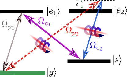
Figure 2: Transfer of OAM from the control field $\Omega_{c_{2}}$ to the second generated probe field $\Omega_{p_{2}}$.

The intensity distributions and the corresponding helical phase pattern of the generated second probe vortex beam $\Omega_{p_{2}}$ are shown in Fig. 3 for different topological charge numbers and under the resonance condition $\delta=0$. When $l=1$, a doughnut intensity profile is observed with a dark hollow center (Fig. 3 (a)). The phase pattern corresponding to this case is plotted in Fig. 3(b). One can see that the phase jumps from $0$ to $2\pi$ around the singularity point. When the OAM number $l$ increases to larger number $l=2$ ($l=3$), the dark hollow center is increased in size as shown in Fig. 3(c) (Fig. 3(e)), while the phase jumps from $0$ to $4\pi$ ($6\pi$) around the singularity point, as can be seen in Fig. 3(d) (Fig. 3(f)).

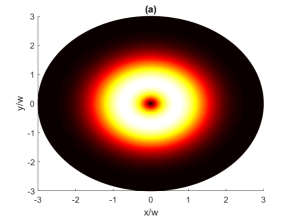
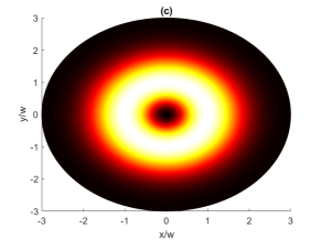
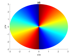
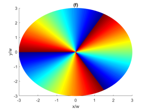
Figure 3: Intensity distributions (a, c, e) in arbitrary units as well as the corresponding helical phase patterns (b, d, f) of the generated second probe vortex beam $\Omega_{p_{2}}$ with different OAM numbers $l=1$ (a, b), $l=2$ (c, d) and $l=3$ (e, f). Here the parameters are $|\Omega_{c_{1}}|=\varepsilon_{c_{2}}=\Gamma$, $\delta=0$, $\Omega_{p_{1}}(0)=0.1\Gamma$, $z=L$ and $\alpha=100$. The position is plotted in dimensionless units.

V Estimation of losses

At the beginning of the atomic medium where the first probe beam $\Omega_{p_{1}}$ has just entered, the second probe beam has not yet been generated ($\Omega_{p_{2}}(0)=0$), so it is not yet driving the transition $|g\rangle\leftrightarrow|e_{2}\rangle$. In this situation, the four-level DL level scheme reduces to an $N$-type atom-light coupling scheme for which a strong absorption is expected Sheng et al. (2011). Going deeper into the atomic medium, the second probe beam is created (see Eq. (16)), resulting in reduction of absorption losses. Yet the losses by absorption are nonzero. It has been shown that the non-degenerate forward FWM in the DL medium can generate strong quantum correlations between twin beams of light in the DL level structure which minimizes the absorption losses McCormick et al. (2007). The amount of phase mismatch in the DL system has been also demonstrated to play an important role to achieve the physical situations in which these losses are minimal Turnbull et al. (2013). In what fallows we will estimate such energy losses, aiming at reaching an optimum condition when the efficiency of the generated probe field is maximum whereas the losses are minimum. Substituting Eqs. (15) and (16) into Eqs. (7) and (8), one gets

$$\rho_{e_{1}g}= \frac{-\Omega_{p_{1}}(0)}{i\Gamma\left(|\Omega_{c_{1}}|^{2}+\varepsilon_{c_{2}}^{2}\left(\frac{r}{w}\right)^{2|l|}\exp\left(-2\frac{r^{2}}{w^{2}}\right)\right)+2\delta|\Omega_{c_{1}}|^{2}}\varepsilon_{c_{2}}^{2}\left(\frac{r}{w}\right)^{2|l|}\exp\left(-\left(2\frac{r^{2}}{w^{2}}+i\frac{\alpha z}{2Ld}\right)\right),$$ (17)

$$\rho_{e_{2}g}= \frac{\Omega_{p_{1}}(0)}{i\Gamma\left(|\Omega_{c_{1}}|^{2}+\varepsilon_{c_{2}}^{2}\left(\frac{r}{w}\right)^{2|l|}\exp\left(-2\frac{r^{2}}{w^{2}}\right)\right)+2\delta|\Omega_{c_{1}}|^{2}}|\Omega_{c_{1}}|\varepsilon_{c_{2}}\left(\frac{r}{w}\right)^{|l|}\exp\left(-\left(\frac{r^{2}}{w^{2}}+i\frac{\alpha z}{2Ld}\right)\right)\exp(il\Phi).$$ (18)

The density matrix elements $\rho_{e_{1}g}$ and $\rho_{e_{2}g}$ generally describe the amplitudes of the excited states $|e_{1}\rangle$ and $|e_{2}\rangle$, respectively. Therefore Eqs. (17) and (18) represent the occupation of excited states inside the medium. It is seen that the losses appear mostly at the beginning of the medium, when going through the medium the losses reduce. In addition, when $r\rightarrow 0$ both Eqs. (17) and (18) are zero indicating that at the vortex core we have no losses. However, away from the vortex core, these equations indicate that the excited states $|e_{1}\rangle$ and $|e_{2}\rangle$ are occupied resulting in absorption losses. Also it follows from Eqs. (17) and (18) that the one-photon detuning $\delta$ plays a critical role in reducing the losses. For the detuning much larger than $\Gamma$ the denominator of Eqs. (17) and (18) becomes very large making negligible occupation of excited states and giving rise to very small losses. However, a large detuning alone may make creation of second probe field less efficient, as indicated by Eq. (16). The latter equation demonstrates that the FWM efficiency can be enhanced by increasing the optical density $\alpha$ . One can conclude that the large detuning requires larger optical density $\alpha$. Yet the optical density $\alpha$ of the atomic cloud is constrained due to neglecting the diffraction terms in the wave equations (5) and (6) Ruseckas et al. (2013). Since the optical density $\alpha$ is proportional to the medium length $L$ and the number density of atoms $n$, the restrictions on the length of the medium limits also the optical density.

It appears that for a given optical density $\alpha$ there is an optimal value of one-photon detuning $\delta$ for which the intensity of second probe field $|\Omega_{p_{2}}|^{2}$ is the maximum. In the following we calculate an analytical expression for optimal $\delta$. From Eq. (11), it is straightforward to obtain the expression for the real-valued quantity $|\Omega_{p_{2}}|^{2}$

$$|\Omega_{p_{2}}|^{2}=|\beta|^{2}\left[1+\exp\left(\frac{-2x}{1+y^{2}\delta^{2}}\right)-2\cos\frac{y\delta x}{1+y^{2}\delta^{2}}\exp\left(\frac{-x}{1+y^{2}\delta^{2}}\right)\right]\,,$$ (19)

where $|\beta|^{2}=\frac{|\Omega_{p_{1}}(0)|^{2}}{|\Omega|^{4}}|\Omega_{c_{1}}|^{2}|\Omega_{c_{2}}|^{2}$, $x=\alpha z/2L$, and $y=2|\Omega_{c_{1}}|^{2}/\Gamma|\Omega|^{2}$. Calculating the derivative of Eq. (19) with respect to $\delta$ we get

$$\frac{\partial|\Omega_{p_{2}}|^{2}}{\partial\delta}=\frac{2xy|\beta|^{2}\exp\left(\frac{-2x}{1+y^{2}\delta^{2}}\right)\left(2y\delta+\exp\left(\frac{x}{1+y^{2}\delta^{2}}\right)\left(-2y\delta\cos\left(\frac{xy\delta}{1+y^{2}\delta^{2}}\right)+(1-y^{2}\delta^{2})\sin\left(\frac{xy\delta}{1+y^{2}\delta^{2}}\right)\right)\right)}{(1+y^{2}\delta^{2})^{2}}.$$ (20)

The optimal detuning $\delta$ is found when

$$2y\delta+\exp\left(\frac{x}{1+y^{2}\delta^{2}}\right)\left(-2y\delta\cos\left(\frac{xy\delta}{1+y^{2}\delta^{2}}\right)+(1-y^{2}\delta^{2})\sin\left(\frac{xy\delta}{1+y^{2}\delta^{2}}\right)\right)=0\,.$$ (21)

Assuming that $\delta$ is sufficiently large ($\delta\gg\Gamma$), we can expand Eq. (21) into Taylor series, yielding

$$\delta\approx\pm\frac{1}{\sqrt{6}}\frac{x}{y},$$ (22)

or, in terms of the physical quantities,

$$\delta\approx\pm\frac{z\Gamma|\Omega|^{2}}{4\sqrt{6}L|\Omega_{c_{1}}|^{2}}\alpha.$$ (23)

Equation (23) provides the values for optimal $\delta$ for which the efficiency of generation of $\Omega_{p_{2}}$ is the largest. According to Eq. (23) the optimal $\delta$ increases linearly with the optical density $\alpha$. Since $\Omega_{c_{2}}$ represents an optical vortex, the ratio $|\Omega|^{2}/|\Omega_{c_{1}}|^{2}$ is not a constant and depends on $r$. In order to estimate an approximate value for the optimal detuning $\delta$ we take the value of $|\Omega|^{2}/|\Omega_{c_{1}}|^{2}$ at the position $r$ of the maximum of $|\Omega_{c_{2}}|$. The dependence of $|\Omega_{c_{2}}|/|\Omega_{c_{1}}|$ on the dimensionless distance from the vortex core $r/w$ is plotted in Fig. 4 by using Eq. (13) and for different OAM numbers $l=1,2,3$. Subsequently the maximum of the quantity $|\Omega_{c_{2}}|/|\Omega_{c_{1}}|$ ($|\Omega_{c_{2}}|_{max}/|\Omega_{c_{1}}|$) and the calculated $|\Omega|^{2}/|\Omega_{c_{1}}|^{2}$ and $\delta$ at $|\Omega_{c_{2}}|_{\mathrm{max}}$ for different $l$ numbers are given in Table 1. One can see, for example, that the maximum of $|\Omega_{c_{2}}|/|\Omega_{c_{1}}|$ for $l=1$ is about $0.42$. In this case, $|\Omega|^{2}/|\Omega_{c_{1}}|^{2}\approx 1.17$, yielding $\delta\approx\pm 11.9\Gamma$. This is an approximate value for the one-photon detuning $\delta$ for which the intensity of second probe field $|\Omega_{p_{2}}|^{2}$ carrying an optical vortex with $l=1$ is the largest, yet the losses are minimum.

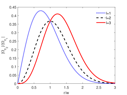
Figure 4: Dependence of the dimensionless quantity $|\Omega_{c_{2}}|/|\Omega_{c_{1}}|$ given in Eq. (13) on the dimensionless distance from the vortex core $r/w$ when $|\Omega_{c_{1}}|=\varepsilon_{c_{2}}=\Gamma$ and for different $l$ numbers.

Table 1: The calculated values for $|\Omega_{c_{2}}|_{max}/|\Omega_{c_{1}}|$, $|\Omega|^{2}/|\Omega_{c_{1}}|^{2}$ and Optimal $\delta$ for different OAM numbers.

	$l=1$	$l=2$	$l=3$
$|\Omega_{c_{2}}|_{max}/|\Omega_{c_{1}}|$	$0.42$	$0.36$	$0.4$
$|\Omega|^{2}/|\Omega_{c_{1}}|^{2}$	$1.17$	$1.13$	$1.16$
Optimal $\delta$	$\pm 11.9\Gamma$	$\pm 11.53\Gamma$	$\pm 11.83\Gamma$

The intensity distribution as well as the phase pattern profiles of the generated vortex beam described by Eq. 16 are plotted in Fig. 5 using Table 1 and for different OAM numbers $l=1,2$ and $3$. As can be seen in Fig. 5 (a, c, e), the intensity distributions are very similar to the patterns displayed for the resonance one-photon detuning $\delta$ (Figs. 3(a,c,e)). As illustrated in Fig.  5 (b, d, f), the phase patterns are bended compared to the resonance case (Figs. 3 (b, d, f)). When $\delta$ is nonzero, the term $\exp[-i\alpha z/(2Ld)]$ in Eq. 16 modulates the phase patterns since it contains $|\Omega_{c_{2}}|$ which is not uniform in $(x,y)$ resulting in bending of phase patterns.

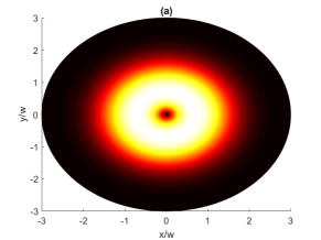
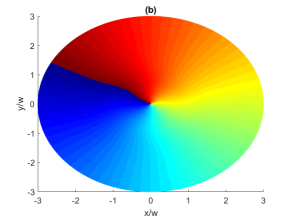
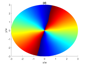
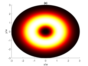
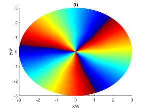
Figure 5: Intensity distributions (a, c, e) in arbitrary units as well as corresponding helical phase patterns (b,d,f)) of the generated second probe vortex beam $\Omega_{p_{2}}$ with different OAM numbers $l=1$ (a,b), $l=2$ (c,d) and $l=3$ (e,f). Here $\delta=11.9\Gamma$ (a, b), $\delta=11.53\Gamma$ (c, d), $\delta=11.83\Gamma$ (e, f) and the parameters are the same as Fig. 3. The position is plotted in dimensionless units.

VI Influence of phase mismatch

In this Section we will investigate the influence of phase mismatch on the exchange of optical vortices. In order to include the effect of phase mismatch we need to add an additional term to the Eq. (6). We introduce the geometrical phase mismatch

$$\Delta_{k}=(k_{p_{1}}-k_{c_{1}}+k_{c_{2}}-k_{p_{2}})\cdot\hat{e}_{z},$$ (24)

where $\hat{e}_{z}$ is the unit vector along the $z$ axis and $k_{p_{1}}$, $k_{p_{2}}$, $k_{c_{1}}$ and $k_{c_{2}}$ are the wave-vectors of the light beams. We consider the situation when all the light beams are co-propagating in the same direction. Note, that the phase mismatch $\Delta_{k}$ can be minimized by introducing a small angle between the propagation directions of the beams. For example, in Ref. Lee et al. (2014) the value of $\Delta_{k}L=0.6$ has been achieved. In the case of non-zero $\Delta_{k}$ instead of Eq. (6) we have Braje et al. (2004)

$$\frac{\partial\Omega_{p_{2}}}{\partial z}+c^{-1}\frac{\partial\Omega_{p_{2}}}{\partial t}+i\Delta_{k}\Omega_{p_{2}}=i\frac{\alpha\gamma_{e_{2}}}{2L}\rho_{e_{2}g}\,.$$ (25)

Substituting Eqs. (7) and (8) into the Maxwell equations (5) and (25) and for $\Omega_{p_{2}}(0)=0$ we get

$$\Omega_{p_{1}}(z)= \frac{1}{s_{1}-s_{2}}\left((q_{1}-s_{2})\exp(s_{1}z)+(s_{1}-q_{1})\exp(s_{2}z)\right)\Omega_{p_{1}}(0),$$ (26)

$$\Omega_{p_{2}}(z)= \frac{1}{q_{2}}\frac{s_{1}-q_{1}}{s_{1}-s_{2}}\left((q_{1}-s_{2})\exp(s_{1}z)+(s_{2}-q_{1})\exp(s_{2}z)\right)\Omega_{p_{1}}(0),$$ (27)

where

$$q_{1}= \frac{-i\alpha}{2Ld}\frac{|\Omega_{c_{2}}|^{2}}{|\Omega|^{2}},$$ (28)

$$q_{2}= \frac{i\alpha}{2Ld}\frac{\Omega_{c_{1}}\Omega_{c_{2}}^{*}}{|\Omega|^{2}},$$ (29)

and

$$s_{1}= \frac{1}{2}\left(-(\frac{i\alpha}{2Ld}+i\Delta_{k})+\sqrt{(\frac{i\alpha}{2Ld}+i\Delta_{k})^{2}+4(\frac{\alpha\Delta_{k}}{2Ld}\frac{|\Omega_{c_{2}}|^{2}}{|\Omega|^{2}})}\right),$$ (30)

$$s_{2}= \frac{1}{2}\left(-(\frac{i\alpha}{2Ld}+i\Delta_{k})-\sqrt{(\frac{i\alpha}{2Ld}+i\Delta_{k})^{2}+4(\frac{\alpha\Delta_{k}}{2Ld}\frac{|\Omega_{c_{2}}|^{2}}{|\Omega|^{2}})}\right).$$ (31)

One can show that when $\Delta_{k}=0$, Eqs. (26) and (27) reduce to Eqs. (10) and (11). However, the analytical expressions given in Eqs. (26) and (27) in presence of the phase mismatch $\Delta_{k}$ are too complicated to see if the OAM of the control field $\Omega_{c_{2}}$ is transferred to the second generated probe beam $\Omega_{p_{2}}$. Hence, we follow the numerical approach to analyze whether or not the exchange of optical vortices is possible.

When $z=L$ and using Eqs. (12)–(14) and Eqs. (28)–(29) we can rewrite Eqs. (26) and (27) as

$$\Omega_{p_{1}}(z=L)= \frac{\Omega_{p_{1}}(0)}{S_{1}-S_{2}}\left[-\left(\frac{i\alpha}{d}\frac{\varepsilon_{c_{2}}^{2}\left(\frac{r}{w}\right)^{2|l|}\exp\left(-2\frac{r^{2}}{w^{2}}\right)}{|\Omega_{c_{1}}|^{2}+\varepsilon_{c_{2}}^{2}\left(\frac{r}{w}\right)^{2|l|}\exp\left(-2\frac{r^{2}}{w^{2}}\right)}+S_{2}\right)\exp(S_{1})\right.$$

$$\left.+\left(\frac{i\alpha}{d}\frac{\varepsilon_{c_{2}}^{2}\left(\frac{r}{w}\right)^{2|l|}\exp\left(-2\frac{r^{2}}{w^{2}}\right)}{|\Omega_{c_{1}}|^{2}+\varepsilon_{c_{2}}^{2}\left(\frac{r}{w}\right)^{2|l|}\exp\left(-2\frac{r^{2}}{w^{2}}\right)}+S_{1}\right)\exp(S_{2})\right],$$ (32)

$$\Omega_{p_{2}}(z=L)= \frac{-i\Omega_{p_{1}}(0)}{S_{1}-S_{2}}\frac{\left[S_{1}d\left(|\Omega_{c_{1}}|^{2}+\varepsilon_{c_{2}}^{2}\left(\frac{r}{w}\right)^{2|l|}\exp\left(-2\frac{r^{2}}{w^{2}}\right)\right)+i\alpha\varepsilon_{c_{2}}^{2}\left(\frac{r}{w}\right)^{2|l|}\exp\left(-2\frac{r^{2}}{w^{2}}\right)\right]}{\alpha|\Omega_{c_{1}}|\varepsilon_{c_{2}}\left(\frac{r}{w}\right)^{|l|}\exp\left(-\frac{r^{2}}{w^{2}}\right)\exp(-il\Phi)}$$

$$\times\left(S_{2}+\frac{i\alpha}{d}\frac{\varepsilon_{c_{2}}^{2}\left(\frac{r}{w}\right)^{2|l|}\exp\left(-2\frac{r^{2}}{w^{2}}\right)}{|\Omega_{c_{1}}|^{2}+\varepsilon_{c_{2}}^{2}\left(\frac{r}{w}\right)^{2|l|}\exp\left(-2\frac{r^{2}}{w^{2}}\right)}\right)(\exp(S_{2})-\exp(S_{1})),$$ (33)

where

$$S_{1}= -(\frac{i\alpha}{2d}+i\Delta_{k}L)+\sqrt{\left(\frac{i\alpha}{2d}+i\Delta_{k}L\right)^{2}+4\left(\frac{\alpha\Delta_{k}L}{2d}\frac{\varepsilon_{c_{2}}^{2}\left(\frac{r}{w}\right)^{2|l|}\exp\left(-2\frac{r^{2}}{w^{2}}\right)}{|\Omega_{c_{1}}|^{2}+\varepsilon_{c_{2}}^{2}\left(\frac{r}{w}\right)^{2|l|}\exp\left(-2\frac{r^{2}}{w^{2}}\right)}\right)},$$ (34)

$$S_{2}= -(\frac{i\alpha}{2d}+i\Delta_{k}L)-\sqrt{\left(\frac{i\alpha}{2d}+i\Delta_{k}L\right)^{2}+4\left(\frac{\alpha\Delta_{k}L}{2d}\frac{\varepsilon_{c_{2}}^{2}\left(\frac{r}{w}\right)^{2|l|}\exp\left(-2\frac{r^{2}}{w^{2}}\right)}{|\Omega_{c_{1}}|^{2}+\varepsilon_{c_{2}}^{2}\left(\frac{r}{w}\right)^{2|l|}\exp\left(-2\frac{r^{2}}{w^{2}}\right)}\right)}.$$ (35)

In Fig. 6, we plot the helical phase pattern of the generated probe beam $\Omega_{p_{2}}(z=L)$ for $\Delta_{k}L=1$ (a, b,c) and $\Delta_{k}L=10$ (d,e,f) and for different OAM numbers $l=1$ (a,d), $l=2$ (b,e) and $l=3$ (c,f). The singularity point appears obviously in phase patterns indicating that the exchange of optical vortices is done and hence, the second probe beam $\Omega_{p_{2}}$ has obtained the OAM of the control field $\Omega_{c_{2}}$ in presence of the phase mismatch $\Delta_{k}$.

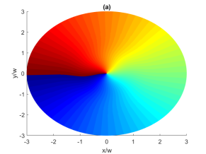
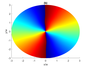
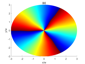
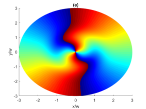
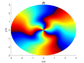
Figure 6: Helical phase patterns of the generated second probe vortex beam $\Omega_{p_{2}}$ described by Eq. (33) for different OAM numbers $l=1$ (a,d), $l=2$ (b,e) and $l=3$ (c,f). Here $\Delta_{k}L=1$ (a, b,c) and $\Delta_{k}L=10$ (d,e,f) and the parameters are the same as Fig. 3. The position is plotted in dimensionless units.

In order to inspect the influence of the phase mismatch on efficiency of OAM transfer, we plot in Fig. 7 the intensities $|\Omega_{p_{1}}|^{2}/|\Omega_{p_{1}}(0)|^{2}$ and $|\Omega_{p_{2}}|^{2}/|\Omega_{p_{1}}(0)|^{2}$ in the whole range of distance $r$ for different values of $\Delta_{k}L$. For small values of $\Delta_{k}L$, the influence of phase mismatch is not significant, yet they are seen to decrease the maximum amplitude of the second generated probe beam for larger values of $\Delta_{k}L$.

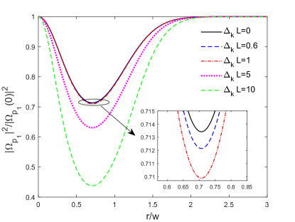
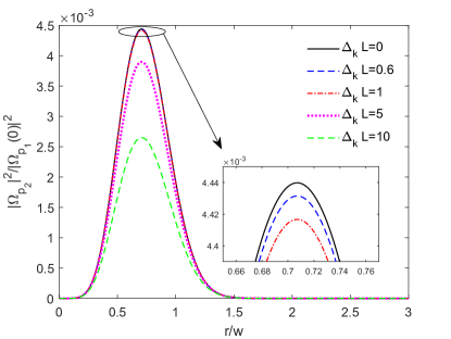
Figure 7: Dependence of the dimensionless quantities $|\Omega_{p_{1}}|^{2}/|\Omega_{p_{1}}(0)|^{2}$ (a) and $|\Omega_{p_{2}}|^{2}/|\Omega_{p_{1}}(0)|^{2}$ (b) given in Eqs. (32) and (33) on the dimensionless distance from the vortex core $r/w$ for different values of $\Delta_{k}L$. Here, $l=1$ and the parameters are the same as Fig. 3.

VII Concluding Remarks

We have considered propagation of slow light with the OAM in a four-level double-$\Lambda$ scheme of atom-light coupling. The medium is illuminated by a pair of probe fields of weaker intensity as well as two control fields with higher intensity. One of the control fields is allowed to carry an OAM, while the second control field is a non vortex beam. The intensity of one of the probe fields is zero at the entrance. The generated probe field acquires the same OAM during the propagation. Yet the presence of a non-vortex control beam makes the total intensity of the control lasers not zero at the vortex core, preventing the absorption losses. As a result, the OAM of the control field can be transferred from the control field to a second generated probe field through a FWM process and without switching on and off of the control fields. Such a mechanism of OAM transfer is much simpler than the previously considered double-tripod scheme where the exchange of vortices is possible only when two control fields carry optical vortices of opposite helicity. The energy losses during such an OAM transfer is then calculated, and the analytical expression for the approximate optimal one-photon detuning is obtained for which the efficiency of generated probe field is maximum while the energy losses are minimal.

Such an EIT based FWM setup can be implemented experimentally for example using the ${}^{87}Rb$ atoms to form a DL level scheme. The ground level $|g\rangle$ can then correspond to the $|5S_{1/2},F=1,m_{F}=0\rangle$ hyperfine state. The lower state $|s\rangle$ can be attributed to the $|5S_{1/2},F=2,m_{F}=0\rangle$ state, whereas we can choose the two excited states $|e_{1}\rangle$ and $|e_{2}\rangle$ as: $|e_{1}\rangle=|5P_{1/2},F=2,m_{F}=1\rangle$ and $|e_{2}\rangle=|5P_{3/2},F=2,m_{F}=1\rangle$.