Ordered arrays of Baryonic tubes in the Skyrme model in (3+1) dimensions at finite density

Abstract

A consistent ansatz for the Skyrme model in (3+1)-dimensions which is able to reduce the complete set of Skyrme field equations to just one equation for the profile in situations in which the Baryon charge can be arbitrary large is introduced: moreover, the field equation for the profile can be solved explicitly. Such configurations describe ordered arrays of Baryonic tubes living in flat space-times at finite density. The plots of the energy density (as well as of the Baryon density) clearly show that the regions of maximal energy density have the shape of a tube: the energy density and the Baryon density depend periodically on two spatial directions while they are constant in the third spatial direction. Thus, these topologically non-trivial crystal-like solutions can be intepreted as configurations in which most of the energy density and the baryon density are concentrated within tube-shaped regions. The positions of the energy-density peaks can be computed explicitly and they manifest a clear crystalline order. A non-trivial stability test is discussed.

1 Introduction

A theoretical description of cold and dense nuclear matter as a function of baryon number density [1] [2] is still lacking. Analytic solutions in the low-energy limit of QCD able to describe crystals-like structures in Baryonic matter at finite density would be extremely helpful in this respect. Until quite recently, the only theoretical arguments supporting the appearance of Baryonic crystals at finite density could be found in two-dimensional effective toy models (see [3], [4] and references therein) as well as in the case of the so-called magnetic Skyrmions [6]. Clever approximations related to either the so-called product ansatz or to Yang-Mills instantons may lead to analytic results in (3+1)-dimensions [5] [7] [8] [9] [10] [11] [12] [13] [14] which help to clarify many properties of these multi-solitonic configurations. In fact, it is still an open problem to build crystals of Baryons explicitly in the low-energy limit of QCD. For this reason, different schemes to describe this phase have been introduced.

A common approach (based on the AdS/CFT correspondence [15]) is in the references [16] [17] [18] [19] [20]. The main difficulty in these cases is to calculate the required solitons: only single baryon solutions have been discussed in details [21] [22]. Numerical solutions at finite density in full Sakai-Sugimoto model are extremely difficult (see [23] [24]).

Despite that, it has been argued that baryons in such a regime are necessarily in a solid crystalline phase [19] [25] [26] [27]. More complex ordered structures are also expected to appear at finite densities. It is widely accepted that the so-called nuclear pasta phase do exist (see [28] [29] [30] [31] and references therein). In this phase, the energy-density plots in the references just mentioned show, for instance, that ordered configurations of ”Baryonic tubes” (nuclear spaghetti) in which most of the Baryonic charge is gathered in tube-shaped regions are observed (nuclear lasagna and nuclear gnocchi phases have also been observed). It is usually assumed that the available theoretical tools are unsuitable to describe such complex structures in the low energy limit of (only numerical results are available in the nuclear pasta phase).

An explicit analytic approach to describe the predictions above in the context of the low energy limit of (3+1)-dimensional QCD is the main goal of the present paper.

The Skyrme theory represents such low energy limit [32] (for detailed reviews on Skyrme theory see [33] [34]). Its topological solitons (called Skyrmions) represent Baryons (see [35] [36] [37] and references therein). The wide range of applications of this theory in many different fields (see [43], [44], [45], [46], [47] and references therein) is well recognized.

The appearance of crystal-like structures in the Skyrme model (which was predicted on the basis of the product ansatz introduced in [7]) is well established numerically (see [34] [38] and references therein). Within the rational map approach [38] one can construct numerically configurations in which the number of ”bumps” in the energy density is related with the corresponding Baryon charge. Based on the fact that, in the Skyrme model, the solution representing one spherical Skyrmion (introduced by Skyrme himself) must be found numerically, it has been always assumed that it is impossible to find analytic solutions representing ordered pattern of solitons without approximations. Consequently, interesting modifications of the original Skyrme model have been considered which do allow to find analytic solutions representing Skyrmions at finite Baryon density (see, in particular, [39] [40] [41] [42] and references therein). However, only the original Skyrme model (which is directly related with the low energy limit of QCD) will be considered here.

The generalized hedgehog ansatz introduced in [48] [49] [50] [51] [52] [53] [54] [55] [56] allowed the construction of the first analytic multi-Skyrmions at finite density (however, these Skyrmions at finite density do not have crystal-like structure).

In the present paper, the methods in [54] [55] [56] will be generalized to construct ordered arrays of Baryonic tubes with crystalline structure living at finite density. One then observes transitions in which for fixed total topological charge, configurations with taller tubes but a smaller number of tubes are energetically favored over configurations made of a lower tubes but with a higher number of tubes.

This paper is organized as follows: in the second section the Skyrme model is introduced and the Skyrme field equations are written in two equivalent ways: this is very important in order to check that the present crystals are really solutions of the full Skyrme field equations. In the third section, the method to go beyond the spherical hedgehog ansatz is introduced and the analytic crystal-like Skyrmions are derived. In the fourth section the appearance of fractional Baryonic charge is discussed. In the final section, some conclusions will be drawn.

2 Beyond the spherical hedgehog ansatz

The action of the $SU(2)$ Skyrme system is

$$S_{Sk} =\frac{K}{2}\int d^{4}x\sqrt{-g}\,\mathrm{Tr}\left(\frac{1}{2}L^{\mu}L_{\mu}+\frac{\lambda}{16}F_{\mu\nu}F^{\mu\nu}\right)\ \ \ K>0\ ,\ \ \ \lambda>0\ ,$$ (1)

$$L_{\mu} :=U^{-1}\nabla_{\mu}U=L_{\mu}^{j}t_{j}\ ,\ \ F_{\mu\nu}:=\left[L_{\mu},L_{\nu}\right]\ ,\ \ \ \hbar=1\ ,\ \ \ c=1\ ,$$

where $K$ and $\lambda$ are the coupling constants, $\mathbf{1}_{2}$ is the $2\times 2$ identity matrix and the $t^{j}$ are the basis of the $SU(2)$ generators (where the Latin index $j$ corresponds to the group index).

The three coupled Skyrme field equations can be obtained by taking the variation of the action with respect to the $SU(2)$-valued field $U$:

$$\frac{\delta S_{Sk}}{\delta U}=0\Leftrightarrow\nabla^{\mu}L_{\mu}+\frac{\lambda}{4}\nabla^{\mu}[L^{\nu},F_{\mu\nu}]=E^{j}t_{j}=0\ ,\ j=1,2,3.$$ (2)

The energy density (the $0-0$ component of the energy-momentum tensor) reads

$$T_{00}=-\frac{K}{2}\mathrm{Tr}\left[L_{0}L_{0}-\frac{1}{2}g_{00}L^{\alpha}L_{\alpha}\,+\frac{\lambda}{4}\left(g^{\alpha\beta}F_{0\alpha}F_{0\beta}-\frac{g_{00}}{4}F_{\sigma\rho}F^{\sigma\rho}\right)\right]\ .$$ (3)

The following parametrization of the $SU(2)$-valued scalar $U(x^{\mu})$ will be adopted

$$U^{\pm 1}(x^{\mu}) =\cos\left(\alpha\right)\mathbf{1}_{2}\pm\sin\left(\alpha\right)n^{i}t_{i}\ ,\ \ n^{i}n_{i}=1\ ,$$ (4)

$$n^{1} =\sin F\cos G\ ,\ \ n^{2}=\sin F\sin G\ ,\ \ n^{3}=\cos F\ ,$$ (5)

$$\alpha =\alpha\left(x^{\mu}\right)\ ,\ F=F\left(x^{\mu}\right)\ ,\ G=G\left(x^{\mu}\right)$$ (6)

where, generically, $\alpha$, $F$ and $G$ are functions of the four space-time coordinates.

It is worth to emphasize here a relevant technical point. The number of Skyrme field equations is equal to the dimension of the corresponding Lie Algebra (in the present case the $SU(2)$ case will be considered so that the task is to solve three coupled non-linear field equations). One can write down the complete set of Skyrme field equations in many different equivalent ways. In this paper two natural representations of the field equations will be considered. The first one is described in Eq. (2). In this matrix representation the three field equations (namely, $E^{j}=0$, $j=1$, $2$, $3$) are obtained as variation of the action with respect to the $SU(2)$-valued scalar field $U$. An equivalent way (which will be described in the next subsection) corresponds to take the most general representation of $SU(2)$-valued scalar field $U$ in the terms of three scalar degrees of freedom ($\alpha$, $F$ and $G$ defined in Eqs. (4), (5)) and (6)) and replace such general representation of $U$ into the action (which will become an action for the three interacting scalar fields $\alpha$, $F$ and $G$). In this second representation, the three field equations (which will be derived explicitly in the next subsection) will be simply

$$\frac{\delta S_{Sk}}{\delta\alpha}=0\ ,\ \frac{\delta S_{Sk}}{\delta F}=0\ ,\ \frac{\delta S_{Sk}}{\delta G}=0\ .$$

Obviously, the two representations are equivalent (in particular, it will be shown explicitly in both representations that the analytic crystals constructed in the present paper are solutions of the complete set of Skyrme field equations). The only warning is that, in general, the field equations in one representation are linear combinations of the field equations in the second representation.

The most difficult task is to find a good ansatz which keeps alive the non-trivial topological charge and, at the same time, allows for a crystal-like structure in the energy density without making the field equations impossible to solve analytically. It is worth to note that with the usual hedgehog ansatz in [32] (as well as in its finite density generalization [54] [55]) the energy density in Eq. (3) (due to the trace on the internal indices) only depends on the Skyrmion profile. Until now, this fact prevented one from describing analytically multi-solitonic configurations with crystal-like order. It is also interesting to note that the main building blocks of these ordered multi-solitonic structures are not necessarily single nucleons. Indeed, it is widely accepted that the so-called nuclear pasta phase may appear (see [28] [29] [30] [31] and references therein). In this phase one can have, for instance, ordered arrays of ”Baryonic tubes” (nuclear spaghetti) in which the shapes of the regions of maximal energy density and Baryon density are tubes. To describe such configurations one necessarily needs an ansatz in which both the Baryon density and the energy density depend not only on the profile $\alpha$ but also on an extra spatial coordinate.

The Baryon charge of the configuration reads

$$W=B=\frac{1}{24\pi^{2}}\int_{\left\{t=const\right\}}\rho_{B}\ ,$$ (7)

$$\rho_{B}=\epsilon^{ijk}Tr\left(U^{-1}\partial_{i}U\right)\left(U^{-1}\partial_{j}U\right)\left(U^{-1}\partial_{k}U\right)\ .$$ (8)

In terms of $\alpha$, $F$ and $G$, the topological density $\rho_{B}$ reads

$$\rho_{B}=12\left(\sin^{2}\alpha\sin F\right)d\alpha\wedge dF\wedge dG\ ,$$ (9)

so that a necessary condition in order to have non-trivial topological charge is

$$d\alpha\wedge dF\wedge dG\neq 0\ .$$ (10)

From the geometrical point of view the above condition (which simply states that $\alpha$, $F$ and $G$ must be three independent functions) can be interpreted as saying that such three functions ”fill a three-dimensional spatial volume” at least locally. In other words, $d\alpha$, $dF$ and $dG$ can be used as 3D volume form. Hence, the condition in Eq. (10) ensures that the configuration one is interested in describes a genuine three-dimensional object. On the other hand, such a condition is not sufficient in general. One has also to require that the spatial integral of $\rho_{B}$ must be a non-vanishing integer:

$$\frac{1}{24\pi^{2}}\int_{\left\{t=const\right\}}\rho_{B}\in\mathbb{Z}\ .$$ (11)

Usually, this second requirement allows to fix some of the parameters of the ansatz.

From now on, as it is customary in the literature, the terms Skyrmionic crystals (and also crystals of solitons) will refer to smooth regular solutions of Eq. (2) with the properties that both the topological charge (defined in Eqs. (7), (8), (9) and (10)) is non-vanishing and larger than 1 and, moreover, that the local maxima of energy density and Baryon density manifest a crystal-like ordered structure.

2.1 Explicit parametrization

It is useful to write down the Skyrme field equations explicitly in terms of the three scalar degrees of freedom $\alpha$, $F$ and $G$. In this way, it is possible to check directly that the novel ansatz proposed in the present paper is consistent. It is convenient to introduce the following functions $Y^{0}(x^{\mu})$ and $Y^{i}(x^{\mu})$

$$Y^{0} =\cos\alpha,\ Y^{1}=\sin(\alpha)\sin(F)\cos(G),\$$ (12)

$$Y^{2} =\sin(\alpha)\sin(F)\sin(G),\ Y^{3}=\sin(\alpha)\cos(F)\ .$$ (13)

In this way, the most general element $U$ of $SU(2)$ can be written as

$$U=\mathbf{I}Y^{0}+Y^{i}t_{i}\;\;\;;\;\;\;U^{-1}=\mathbf{I}Y^{0}-Y^{i}t_{i}\ .$$

These functions are useful to write down the Skyrme action explicitly in terms of $\alpha$, $F$ and $G$. Introducing the tensor $\Sigma_{\mu\nu}$

$$\Sigma_{\mu\nu}=G_{ij}\nabla_{\mu}Y^{i}\nabla_{\nu}Y^{j}\;\;;\;\;G_{ij}=\delta_{ij}+\frac{Y^{i}Y^{j}}{1-Y^{k}Y_{k}}$$ (14)

the Skyrme action is then defined as

$$I=\int d^{4}x\sqrt{-g}\left[\frac{1}{2}\Sigma_{\mu}^{\mu}+\frac{\lambda}{4}\left((\Sigma_{\mu}^{\mu})^{2}-\Sigma^{\mu\nu}\Sigma_{\mu\nu}\right)\right].$$ (15)

Now, we are in the position to write down the general Skyrme field equations in terms of $\alpha$, $F$ and $G$ (which obviously are equivalent to the Skyrme field equations in matrix form in Eq. (2)). The variation of the Skyrme action with respect to $\alpha$ leads to the equation of motion

$$\begin{array}[c]{c}\left(-\Box\alpha+\sin(\alpha)\cos(\alpha)\left(\nabla_{\mu}F\nabla^{\mu}F+\sin^{2}F\nabla_{\mu}G\nabla^{\mu}G\right)\right)\\ +\lambda\left(\begin{array}[c]{c}\sin(\alpha)\cos(\alpha)\left((\nabla_{\mu}\alpha\nabla^{\mu}\alpha)(\nabla_{\nu}F\nabla^{\nu}F)-(\nabla_{\mu}\alpha\nabla^{\mu}F)^{2}\right)\\ +\sin(\alpha)\cos(\alpha)\sin^{2}(F)\left((\nabla_{\mu}\alpha\nabla^{\mu}\alpha)(\nabla_{\nu}G\nabla^{\nu}G)-(\nabla_{\mu}\alpha\nabla^{\mu}G)^{2}\right)\\ +2\sin^{3}(\alpha)\cos(\alpha)\sin^{2}(F)\left((\nabla_{\mu}F\nabla^{\mu}F)(\nabla_{\nu}G\nabla^{\nu}G)-(\nabla_{\mu}F\nabla^{\mu}G)^{2}\right)\\ -\nabla_{\mu}\left(\sin^{2}(\alpha)(\nabla_{\nu}F\nabla^{\nu}F)\nabla^{\mu}\alpha\right)+\nabla_{\mu}\left(\sin^{2}(\alpha)(\nabla_{\nu}\alpha\nabla^{\nu}F)\nabla^{\mu}F\right)\\ -\nabla_{\mu}\left(\sin^{2}(\alpha)\sin^{2}(F)(\nabla_{\nu}G\nabla^{\nu}G)\nabla^{\mu}\alpha\right)+\nabla_{\mu}\left(\sin^{2}(\alpha)\sin^{2}(F)(\nabla_{\nu}\alpha\nabla^{\nu}G)\nabla^{\mu}G\right)\end{array}\right)\end{array}=0\ ,$$ (16)

The variation of the Skyrme action with respect to $F$ leads to the equation of motion

$$\begin{array}[c]{c}\left(-\sin^{2}(\alpha)\Box F-2\sin(\alpha)\cos(\alpha)\nabla_{\mu}\alpha\nabla^{\mu}F+\sin^{2}(\alpha)\sin(F)\cos(F)\nabla_{\mu}G\nabla^{\mu}G\right)\\ +\lambda\left(\begin{array}[c]{c}\sin^{2}(\alpha)\sin(F)\cos(F)\left((\nabla_{\mu}\alpha\nabla^{\mu}\alpha)(\nabla_{\nu}G\nabla^{\nu}G)-(\nabla_{\mu}\alpha\nabla^{\mu}G)^{2}\right)\\ +\sin^{4}(\alpha)\sin(F)\cos(F)\left((\nabla_{\mu}F\nabla^{\mu}F)(\nabla_{\nu}G\nabla^{\nu}G)-(\nabla_{\mu}F\nabla^{\mu}G)^{2}\right)\\ -\nabla_{\mu}\left(\sin^{2}(\alpha)(\nabla_{\nu}\alpha\nabla^{\nu}\alpha)\nabla^{\mu}F\right)+\nabla_{\mu}\left(\sin^{2}(\alpha)(\nabla_{\nu}\alpha\nabla^{\nu}F)\nabla^{\mu}\alpha\right)\\ -\nabla_{\mu}\left(\sin^{4}(\alpha)\sin^{2}(F)(\nabla_{\nu}G\nabla^{\nu}G)\nabla^{\mu}F\right)+\nabla_{\mu}\left(\sin^{4}(\alpha)\sin^{2}(F)(\nabla_{\nu}F\nabla^{\nu}G)\nabla^{\mu}G\right)\end{array}\right)\end{array}=0\ ,$$ (17)

The variation of the Skyrme action with respect to $G$ leads to the equation of motion

$$\begin{array}[c]{c}\left(-\sin^{2}(\alpha)\sin^{2}(F)\Box G-2\sin(\alpha)\cos(\alpha)\sin^{2}(F)\nabla_{\mu}\alpha\nabla^{\mu}G-2\sin^{2}(\alpha)\sin(F)\cos(F)\nabla_{\mu}F\nabla^{\mu}{G}\right)\\ +\lambda\left(\begin{array}[c]{c}-\nabla_{\mu}\left[\sin^{2}(\alpha)\sin^{2}(F)(\nabla_{\nu}\alpha\nabla^{\nu}\alpha)\nabla^{\mu}G\right]+\nabla_{\mu}\left[\sin^{2}(\alpha)\sin^{2}(F)(\nabla_{\nu}\alpha\nabla^{\nu}G)\nabla^{\mu}\alpha\right]\\ -\nabla_{\mu}\left[\sin^{4}(\alpha)\sin^{2}(F)(\nabla_{\nu}F\nabla^{\nu}F)\nabla^{\mu}G\right]+\nabla_{\mu}\left[\sin^{4}(\alpha)\sin^{2}(F)(\nabla_{\nu}F\nabla^{\nu}G)\nabla^{\mu}F\right]\end{array}\right)\end{array}=0\ .$$ (18)

2.1.1 Example: the original Skyrme ansatz

Here we give a simple and well known example showing that the above equations (16), (17) and (18) are suitable to devise a strategy to find good ansatz which reduce the full Skyrme field equations to only one consistent equation for the profile in a non-trivial topological sector. The original Skyrme ansatz is defined by the choice

$$\alpha=\alpha_{s}(R)\ ,\ F=\theta\ ,\ G=\varphi\ ,$$ (19)

in the flat metric in spherical coordinates:

$$ds^{2}=g_{\mu\nu}dx^{\mu}dx^{\nu}=-dt^{2}+dR^{2}+R^{2}\left(d\theta^{2}+\sin\theta^{2}d\varphi^{2}\right)\ .$$ (20)

One can check that, due to the identities

$$\nabla_{\mu}\alpha_{s}\nabla^{\mu}F=\nabla_{\mu}G\nabla^{\mu}\alpha_{s}=\nabla_{\mu}G\nabla^{\mu}F\ =0\ ,$$ (21)

and to the fact that both $F$ and $G$ are linear functions in the chosen coordinates system, the three Skyrme field equations (16), (17) and (18) reduce to only one consistent scalar equation for the profile $\alpha_{s}(R)$. A crucial technical detail is the following: in the equation for $\alpha_{s}(R)$ (namely, Eq. (16)) potentially dangerous terms are the ones involving $\sin F^{2}$ as these terms involve $\theta$ while one would like to have a consistent equation for $\alpha_{s}(R)$ which, therefore, can only involve $R$-dependence. In the original ansatz of Skyrme the dangerous $\theta-$dependence due to $\sin F^{2}$ is canceled by the inverse metric $g^{\varphi\varphi}$ appearing in $\nabla_{\mu}G\nabla^{\mu}G$. Thus, one can reduce the three Skyrme field equations to a single scalar equation for $\alpha_{s}(R)$. If one plugs the ansatz in Eq. (19) into the three Skyrme field equations (16), (17) and (18) one can see directly that Eqs. (17) and (18) are identically satisfied and that Eq. (16) reduces to the usual equation for the Skyrme profile $\alpha_{s}(R)$ which can be found in all the textbooks (see, for instance, [34]). In the following, a different trick to get a consistent equation for $\alpha$ in a topologically non-trivial sector will be introduced.

2.1.2 Comparison with the rational map ansatz

The idea of the rational map approach [38] is to obtain an approximate description of multi-Skyrmionic configurations replacing the isospin vector $n^{i}$ for the spherical hedgehog defined in Eqs. (5), (19) and (20) by a more general map between two spheres. Even if the rational map ansatz is only an approximation, it provides one with a very clear intuitive picture of multi-Skyrmionic configurations.

The usual starting point is

$$Y^{0}=\cos\alpha\ ,\ \ Y^{i}=\left(n_{\Psi}\right)^{i}\sin\alpha\ ,\ \ \ \alpha=\alpha(R)\ ,\ \ \delta_{ij}\left(n_{\Psi}\right)^{i}\left(n_{\Psi}\right)^{j}=1$$ (22)

$$\left(n_{\Psi}\right)^{1} =\frac{\Psi+\overline{\Psi}}{1+\left|\Psi\right|^{2}}\ ,\ \ \ \left(n_{\Psi}\right)^{2}=\frac{i\left(\Psi-\overline{\Psi}\right)}{1+\left|\Psi\right|^{2}}\ ,\ \ \ \left(n_{\Psi}\right)^{3}=\frac{1-\left|\Psi\right|^{2}}{1+\left|\Psi\right|^{2}}\ ,$$ (23)

$$\Psi =\Psi(z)\ ,\ \ z\in\mathbb{C}\ \ ,$$ (24)

where $z$ is a complex coordinate which, using the stereographic projection, can be identified with the coordinates on the 2-sphere:

$$z=\exp\left(i\varphi\right)\tan\left(\frac{\theta}{2}\right)\ .$$

The rational map $\Psi(z)$ (which gives the name to the whole approach) reads

$$\Psi\left(z\right)=\frac{p\left(z\right)}{q\left(z\right)}\ ,$$

where $p$ and $q$ are polynomials in $z$ with no common factor. The degree $N$ of the rational map $\Psi$ is defined as

$$N=\int\frac{2idzd\overline{z}}{\left(1+\left|z\right|^{2}\right)^{2}}\left(\frac{1+\left|z\right|^{2}}{1+\left|\Psi\right|^{2}}\left|\frac{d\Psi}{dz}\right|\right)^{2}\ .$$ (25)

It is well-known that

$$N=\max\left(n_{p},n_{q}\right)\ ,$$

where $n_{p}$ and $n_{q}$ are the degrees of $p\left(z\right)$ and $q\left(z\right)$ respectively. Correspondingly, the Baryon number $B$ of the configuration in Eqs. (22), (23) and (24) reads

$$B=-\frac{1}{24\pi^{2}}\int\epsilon^{ijk}Tr\left(U^{-1}\partial_{i}U\right)\left(U^{-1}\partial_{j}U\right)\left(U^{-1}\partial_{k}U\right)=nN\ ,$$ (26)

where

$$n=\left(-\frac{2}{\pi}\int\left(\alpha^{\prime}\sin^{2}\alpha\right)dR\right)\ .$$ (27)

The winding number is the product of the contribution coming from the profile function $\alpha$ times the degree $N$ of the rational map $\Psi$. One can think that $n$ is the number of ”bumps” associated to $\alpha$ while $N$ are related to the bumps in the directions orthogonal to $\alpha$.

When (and only when)

$$\Psi=z\ ,$$ (28)

the rational map ansatz in Eqs. (22), (23) and (24) reduces to the original spherical hedgehog ansatz discussed in the previous subsection and it gives rise to a (numerical) solution of the complete set of Skyrme field equations. On the other hand, in all the higher degrees cases $N>1$ the rational map solutions are only approximated solutions of the complete set of Skyrme field equations.

The strategy of this approach is to minimize the total energy with respect to both $\alpha$ and the rational map $\Psi$. This framework is tied to situations in which there is an approximated spherical symmetry: in particular, the crystals-like configurations typical of nuclear pasta (see [28] [29] [30] [31] and references therein) cannot be analyzed in this approach. The main advantage of this rational-map framework is that it disentangles the radial coordinate $R$ from the angular coordinates. The main disadvantage is that, as already emphasized, such a disentangling is only an approximation.

In terms of the explicit parametrization introduced in Eqs. (12) and (13) (in which the complete set of Skyrme field equations are (16), (17) and (18)) one can interpret the rational map approach as follows. The first step of the procedure (in which one minimizes the energy functional with respect to the rational map) gives rise to an effective equation for the radial profile which is very similar to the original one of Skyrme with the difference that some parameters are rescaled (see, in particular, the discussion in [53] and references therein). Thus, in a sense, one can think that in the rational-map approach Eqs. (17) and (18) are solved ”on average” (freezing $\alpha$) and then the corresponding Eq. (16) for $\alpha$ is solved (more often than not) numerically.

Instead, in the present paper it will be introduced an ansatz with three main advantages.

Firstly, the complete set of Skyrme field equations will be solved exactly (and not only approximately). In other words, the ansatz described in the next sections will solve Eqs. (16), (17) and (18) without any approximation.

Secondly, the solutions will be analytical and not numerical.

Thirdly, the ansatz is not tied to situations with spherical symmetry.

3 Skyrme Crystals

The main physical motivation of the present work is to study finite density effects. The easiest way to take into account finite-density effects is to introduce the following flat metric

$$ds^{2}=-dt^{2}+A\left(dr^{2}+d\theta^{2}\right)+L^{2}d\phi^{2}\ ,$$ (29)

where $4\pi^{3}LA$ is the volume of the box in which the Skyrmions configurations to be constructed below will live. The adimensional spatial coordinates $r$, $\theta$ and $\phi$ have the range

$$0\leq r\leq 2\pi\ ,\quad 0\leq\theta\leq\pi\ ,\quad 0\leq\phi\leq 2\pi\ .$$ (30)

Following the strategy of [54] [55], the boundary conditions in the $\theta$ direction here will be chosen to be Dirichlet while in the $r$ and $\phi$ directions they can be both periodic and anti-periodic. These are not the only allowed boundary conditions: however this is the simplest choice as it will be discussed in a moment.

The ansatz for the Skyrme crystal is

$$\alpha=\alpha\left(r\right)\ ,\ F=q\theta\ ,\ G=p\left(\frac{t}{L}-\phi\right)\ ,\ q=2v+1,\quad p,\ v\in\mathbb{N}\ ,\ p\neq 0\ .$$ (31)

The periodic time dependence in Eq. (31) is natural for three very good reasons.

Firstly, the most popular way to avoid Derrick’s famous no-go theorem on the existence of solitons in non-linear scalar field theories corresponds to search for a time-periodic ansatz such that the energy density of the configuration is still static, as it happens for boson stars [57] (in the simpler case of $U(1)$-charged scalar field: see [58] and references therein). The present ansatz defined in Eqs. (4), (5) and (31) has exactly this property. Indeed, the energy density does not depend on time (see Eqs. (44), (45) and (46) below) so that these configurations possess a static energy density.

Secondly, unlike what happens for the usual Bosons star ansatz for $U(1)$-charged scalar fields, the present ansatz for $SU(2)$-valued scalar field also possesses a non-trivial topological charge.

Thirdly, with the above choice of the ansatz the complete set of Skyrme field equations simplifies dramatically (as it will be shown below) due to the fact that, with the function $G$ in Eq. (31), $\nabla_{\mu}G\nabla^{\mu}G=0$.

With the ansatz defined in Eqs. (4), (5) and (31) the topological density in Eq. (8) reads

$$\rho_{B}=\left[\left(12pq\sin\left(q\theta\right)\sin^{2}\alpha\right)\partial_{r}\alpha\right]dr\wedge d\theta\wedge d\phi\ .$$ (32)

The above ansatz satisfies the first condition to be topologically non-trivial in Eq. (10) as the three function $\alpha$, $F$ and $G$ in Eq. (31) are independent and ”fill a three-dimensional space” (see the discussion about Eq. (10)). As far as the boundary conditions are concerned, one can check directly that if one chooses, for instance, periodic boundary conditions in $\theta$ (taking $q$ to be an even number in Eq. (31)) the topological charge vanishes (even if the topological density does not) so that the second condition in Eq. (11) would be violated. Hence, the simplest choice to get topologically non-trivial configurations is to take $q$ to be an odd integer. I hope to come back on the analysis of other possible boundary conditions in a future publication. The boundary condition on $\alpha$ and the corresponding Baryon charge are

$$\alpha\left(2\pi\right)-\alpha\left(0\right)=n\pi\ \Rightarrow\ B=np\ .$$ (33)

Thus, the present ansatz cannot be deformed continuously to the trivial vacuum $U_{0}=\mathbf{1}_{2x2}$ since the third homotopy class (which represents the Baryon charge) is non-vanishing.

3.1 Tube-shaped regions

In order to understand the shape of the regions of maximal Baryon density (which will coincide with the shape of the regions of maximal energy density: see Eqs. (44), (45) and (46) below) one can proceed as follows. The baryon density $\rho_{B}$ in Eqs. (8) and (32) is periodic in $r$ and $\theta$ while it is constant in the $\phi$-direction. One observes that the positions of the maxima of the Baryon density are defined by the conditions

$$\sin^{2}\alpha=1\ ,\ \sin^{2}\left(q\theta\right)=1\ ,$$ (34)

which define a periodic 2-dimensional lattice in $r$ and $\theta$. The contour-plots in Figure 1 for the energy-density have a similar pattern. Since both the Baryon density and the energy density are constant in the third spatial direction $\phi$, a three-dimensional contour plot would show that the shapes of the regions of maximal energy density (and similarly for the Baryon density) are tubes of length $2\pi L$.

In other words, in order to understand the three-dimensional shape of the regions of maximal energy and Baryon density one has simply to take the clear-yellow spots in Figure 1 and move them along the $\phi$-direction (which is orthogonal to the $r-\theta$ plane of Figure 1). Hence, such regions are (ordered arrays of) parallel tubes. The ”$\phi$-constant” sections of these tubes correspond to the contour plots in Figure 1.

3.2 The explicit solution

When one plugs the ansatz in Eq. (31) into the complete set of three coupled Skyrme field equations in Eq. (2), they reduce to only one integrable equation for $\alpha(r)$:

$$E_{j}=c_{j}P\left[\alpha\right]\ ,\ c_{j}\neq 0\ ,\ j=1,2,3,$$ (35)

$$P\left[\alpha\right]=0\Leftrightarrow\partial_{r}\left[Y\left(\alpha\right)\frac{\left(\partial_{r}\alpha\right)^{2}}{2}-V(\alpha)-E_{0}\right]=0\ ,$$ (36)

$$Y\left(\alpha\right)=\left(A+q^{2}\lambda\sin^{2}\alpha\right)\ ,\ V(\alpha)=\frac{q^{2}A}{2}\sin^{2}\alpha\ \Rightarrow$$ (37)

$$\eta\left(\alpha,E_{0}\right)\overset{def}{=}\frac{\left[2\left(E_{0}+V(\alpha)\right)\right]^{1/2}}{Y\left(\alpha\right)^{1/2}}\ \Rightarrow$$ (38)

$$\ \frac{d\alpha}{\eta\left(\alpha,E_{0}\right)} =dr\ ,$$ (39)

where $E_{0}$ is an integration constant to be fixed requiring the boundary condition in Eq. (33). In other words, with the ansatz in Eq. (31) all the three Skyrme field equations in Eq. (2) $E_{j}=0$ have the common factor $P\left[\alpha\right]$ defined in Eq. (36) so that if $P\left[\alpha\right]=0$ then all the Skyrme field equations are satisfied. This is the reason why the ansatz in Eq. (31) has been chosen.

An alternative way to see that the above ansatz reduce the complete set of Skyrme field equations to just one equation for the profile $\alpha$ keeping alive the topological charge is to use the explicit parametrization of the Skyrme action in term of $\alpha$, $F$ and $G$ in Eqs. (12), (14) and (15). In this way, one can read directly the field equations for the three functions $\alpha$, $F$ and $G$. The relevant properties of the ansatz in Eq. (31) are

$$\nabla_{\mu}\alpha\nabla^{\mu}F =\nabla_{\mu}\alpha\nabla^{\mu}G=\nabla_{\mu}G\nabla^{\mu}F=0\ ,$$ (40)

$$\nabla_{\mu}G\nabla^{\mu}G =0\ ,\$$ (41)

$$\rho_{B} \approx 12\left(\sin^{2}\alpha\sin F\right)d\alpha\wedge dF\wedge dG\neq 0\ .$$ (42)

If one takes into account Eqs. (40), (41) and (42) together with the fact that both $F$ and $G$ depend linearly on the coordinates defined in Eqs. (29) and (30), one can see easily that Eqs. (17) and (18) are identically satisfied and that Eq. (16) reduces to Eq. (36) $P\left[\alpha\right]=0$. Thus, unlike what happens in the case of the original spherical Skyrme ansatz discussed in the previous section, in the present case one can reduce the three Skyrme field equations to only one consistent equation for $\alpha(r)$ because the potentially dangerous terms involving $\sin F$ appearing in Eq. (16) are eliminated by the property in Eq. (41).

All in all, the three coupled Skyrme field equations Eq. (2) with the ansatz in Eq. (31) reduce to a simple quadrature which can be integrated using elliptic functions. The boundary condition in Eq. (33) reduces to:

$$\int_{0}^{n\pi}\frac{d\alpha}{\eta\left(\alpha,E_{0}\right)}=n\int_{0}^{\pi}\frac{d\alpha}{\eta\left(\alpha,E_{0}\right)}=2\pi\ ,\ E_{0}>0\ .$$ (43)

The above equation for $E_{0}$ always has a positive real solution. Moreover, one can see that $\partial_{r}\alpha>0$ and that, when $n$ is large, both $\eta\left(\alpha,E_{0}\right)$ and $E_{0}$ are of order $n$.

The conclusion is that the ansatz in Eqs. (4), (5), (6) and (31) in the flat metric in Eqs. (29) and (30) in which the profile $\alpha$ is given in closed form in Eqs. (37), (38), (39) and (43) gives rise to exact and topologically non-trivial solutions (with Baryonic charge $np$) of the complete set of Skyrme field equations for any integers $n$ and $p$ and for any odd integer $q$.

3.3 Energy-density

The energy density (replacing $\left(\partial_{r}\alpha\right)^{2}$ with $\eta\left(\alpha,E_{0}\right)^{2}$ using Eq. (38)) in Eq. (3) with the ansatz in Eq. (31) reads

$$T_{00}=\frac{Kp}{4L^{2}A}\left[2\rho_{0}\left(\alpha\right)+4\sin^{2}\left(q\theta\right)\rho_{1}\left(\alpha\right)\right]\ ,$$ (44)

where

$$\rho_{0}\left(\alpha\right) =\frac{\left(Lq\right)^{2}}{p}\sin^{2}\alpha+\eta\left(\alpha,E_{0}\right)^{2}\left[\frac{\left(L\right)^{2}}{p}+\lambda\frac{\left(Lq\right)^{2}}{Ap}\sin^{2}\alpha\right]\ ,\$$ (45)

$$\rho_{1}\left(\alpha\right) =\sin^{2}\alpha\left[Ap+\lambda q^{2}p\sin^{2}\alpha+\lambda p\eta\left(\alpha,E_{0}\right)^{2}\right]\ .$$ (46)

There are two important differences with respect to the first analytic examples of Skyrmions living at finite density in flat spaces [54] [55] [56].

Firstly, in that references, the factor $\sin 2H$ (where $H$ is the profile defined in Eqs. (9) and (10) of [54]) appears linearly in the Baryon density in Eq. (16) of [54]. Thus, in that references, it is not possible to increase the Baryon charge by increasing the number of ”bumps” in the profile $H$.

Secondly, the energy density (defined in Eq. (15) of [54]) only depends on $H$ (and, consequently, it only depends on one spatial coordinate). This prevents one from describing explicitly crystal-like structures in which the number of bumps in the energy-density is related with the Baryon number (as, in that references, only one bump in $H$ is allowed).

In the present case both problems are solved since in the Baryon density in Eq. (32) $\sin\alpha$ appears quadratically (so that by increasing the number of ”bumps” in $\alpha$ one also increases the Baryon charge) and the energy density in Eqs. (44), (45) and (46) (even after taking the trace over the $SU(2)$ indices) depends non-trivially both on the profile $\alpha$ and on the spatial coordinate $\theta$ (so that a clear crystal-like structure in its peaks emerges).

The two contour plots of the energy-density in the $r-\theta$-plane below in Figure 1 (with $p=1$, $q=1$ and $n=25$ on the left and $p=1$, $q=3$ and $n=25$ on the right) show the crystal-like pattern of the bumps (whose positions can be determined explicitly maximizing the energy-density):

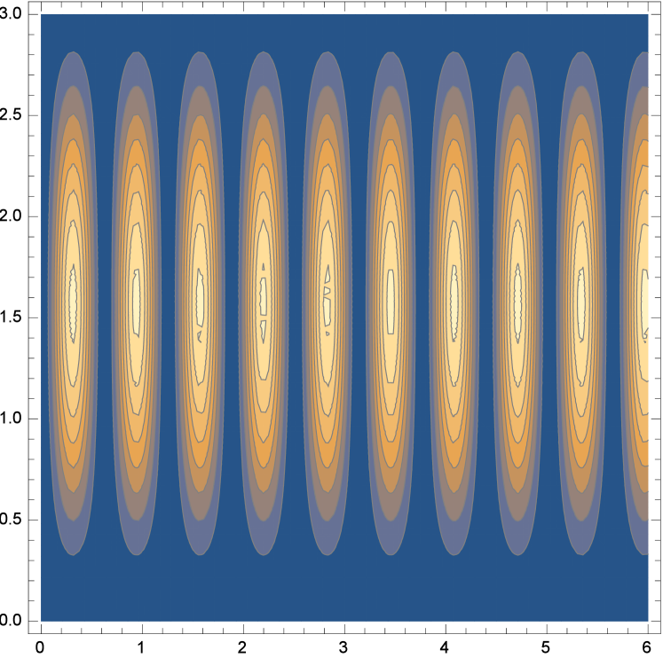
(a) $p=1$, $n=25$ and $q=1$

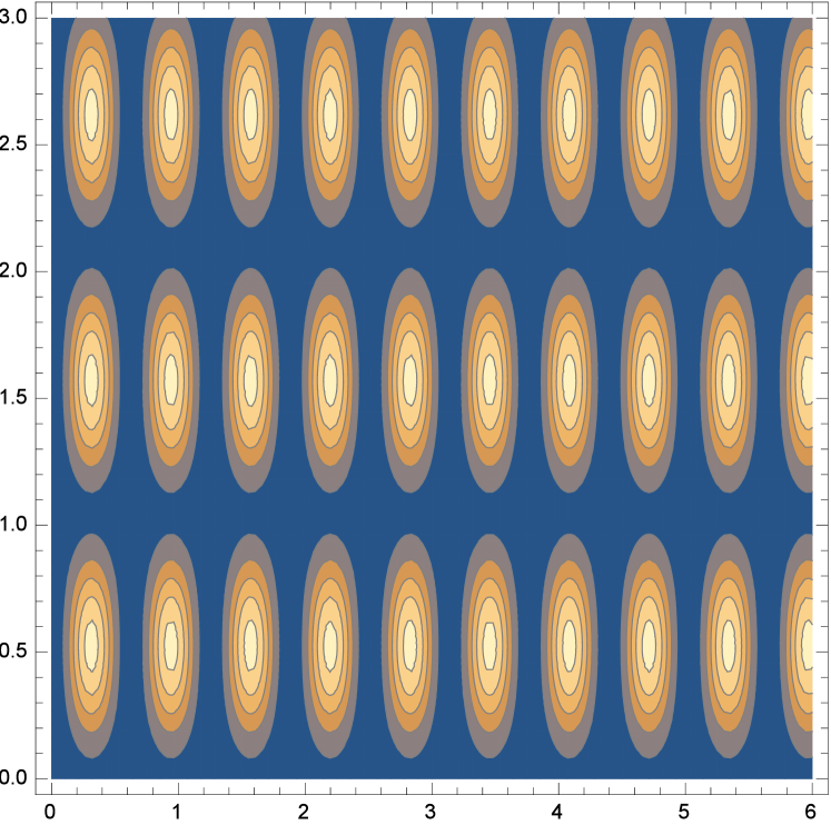
(b) $p=1$, $n=25$ and $q=3$

Figure 1: The left panel (a) shows the contour plot of the energy density with $p=1$, $n=25$ and $q=1$ (where the highest energy density is in clear yellow while the lowest is blue). The right panel (b) shows the contour plot of the energy with $p=1$, $n=25$ and $q=3$ (in both cases it has been assumed that $K=2$ and $\lambda=1$; note that the horizontal axis corresponds to the $r$ direction while the vertical axis to the $\theta$ direction). The patterns of the peaks clearly show a crystal-like structure. It is clear to see that, when passing from $q=1$ to higher values of $q$ (keeping fixed $n$ and $p$), the bumps in the energy density (which, when $q=1$, carry one unit of Baryon charge) are divided into $q$ smaller bumps each of which carries $1/q$ of Baryon charge.

These configurations are ordered arrays of Baryonic tubes (namely, tubes in which most of the energy density and Baryonic charge is concentrated within tube-shaped regions). It is easy to recognize that this is the case since both the energy density and the Baryon density do not depend on the third spatial direction $\phi$  (while they are periodic both in $r$ and in $\theta$). A three-dimensional contour plot would reveal that the clear-yellow regions in Figure 1 of maximal energy density would become, in 3D, clear-yellow tubes. The positions of these Baryonic tubes in the $r-\theta$ plane (defined by the clear-yellow spots in Figure 1) manifest a clear crystalline order. The similarity with the spaghetti-like configurations found (numerically) in the nuclear pasta phase (see the plots in [28] [29] [30] [31] and references therein) is quite amazing.

Consequently, the interpretation of the above results together with the plots in Figure 1 tell that, when $q=1$, the integer $n$ corresponds to the number of Baryonic tubes in the configurations while $p$ is the Baryonic charge of each tube. The role of the integer $q$ will be analyzed in the next section.

The total energy $E_{tot}$ of the configuration can be obtained in a closed form (using Eqs. (38) and (39)). One is left with an integral of an explicitly known function of $\alpha$ which contains all the relevant informations:

$$E_{tot} =\int\sqrt{-g}d^{3}xT_{00}=B\pi^{2}K\int_{0}^{\pi}d\alpha\Omega\left(\alpha;p,q,n\right)\ ,$$ (47)

$$\Omega\left(\alpha;p,q,n\right) =\frac{A\sin^{2}\alpha}{\eta\left(\alpha,E_{0}\right)}\left[\frac{Lq^{2}}{Ap}+\frac{p}{L}+\frac{\lambda pq^{2}}{AL}\sin^{2}\alpha\right]+$$ (48)

$$+\frac{\eta\left(\alpha,E_{0}\right)}{A}\ \left[\frac{AL}{p}+\lambda\sin^{2}\alpha\left(\frac{Lq^{2}}{p}+\frac{Ap}{L}\right)\right]\ ,$$

where $B=np$ is the Baryon number, $n$ is the number of bumps associated with the profile $\alpha$ in the $r$ direction. The above equation represents the explicit expression for the total energy as a function of the parameters of the system. As it was already emphasized in the discussion below Eq. (34), the total energy does not depend on $p$ and $L$ separately but only on the ratio $p/L$.

It is convenient from the energetic point of view neither to have very small $p/L$ nor to have very large $p/L$. This can be seen as follows: let us denote the variable $p/L$ as $\xi$. Then, the total energy per-Baryon (namely, $E_{tot}/B$ from Eqs. (47) and (48)) as function of $\xi$ (assuming that $n$ is large so that $\eta\left(\alpha,E_{0}\right)\sim n$) reads

$$\frac{E_{tot}\left(\xi\right)}{B} =c_{0}\xi+\frac{c_{1}}{\xi}\ ,\ \ \ \xi=\frac{p}{L}\ ,$$ (49)

$$c_{0} >0\ ,\ c_{1}>0\ ,$$ (50)

where $c_{1}$ and $c_{0}$ (which can be read from the explicit expressions in Eqs. (47) and (48)) depend on all the other parameters of the theory. Thus, the total energy per-Baryon as function of $\ \xi$ has a non-trivial local minimum:

$$\xi^{\ast}=\sqrt{\frac{c_{1}}{c_{0}}}\ .$$ (51)

This fact means that if one increases the value of $p$ one also has to increase the length of the tube $L$ in such a way to keep $p/L$ equal to its optimal value in the above equation. Therefore one can interpret $p$ as the length of the Baryonic tubes in unit of $fm$.

A further natural question is the following:

given a total Baryon number $B$, is it energetically more convenient to have higher $p$ and lower $n$ or the other way around?

The answer to this question in the low energy limit of QCD can be found just by analyzing the function $\Omega\left(\alpha;p,q,n\right)$ defined in Eq. (48) which contains all the relevant informations. For instance, can see explicitly that if $A$ decreases it is better to have larger values for $p$.

In other words, if one keeps $B=np$ fixed and $A$ decreases, then it is better to have taller tubes (and a smaller number of tubes to keep $B$ fixed).

On the other hand, if one increases $A$ it is better to have a bigger number of smaller tubes (to keep $B$ fixed). Although a plot of the total energy (or total energy per-Baryon as function of all the parameters is not very useful), if one keeps some of the parameters fixed and only considers pairs of related parameters (such as $p$ and $L$ or $A$ and $n$) the pattern is always similar to the one in Eqs. (49) and (50). I hope to come back on the properties of the function $\Omega\left(\alpha;p,q,n\right)$ defined in Eq. (48) in a future publication.

3.4 A remark on the stability

A remark on the stability of the above crystals is in order. In many situations, when the hedgehog property holds (so that the field equations reduce to a single equation for the profile) the most dangerous perturbations are perturbations of the profile which keep the structure of the ansatz (see [59] [60] and references therein). In the present case these are

$$\alpha\rightarrow\alpha+\varepsilon u\left(r\right)\ ,\ \ \ \varepsilon\ll 1\ .$$ (52)

It is a direct computation to show that the linearized version of Eq. (36) around a background solution $\alpha_{0}\left(r\right)$ of charge $B=np$ always has the following zero-mode: $u\left(r\right)=\partial_{r}\alpha_{0}\left(r\right)$. Due to Eqs. (38), (39) and (43) $u(r)$ has no node so that it must be the perturbation with lowest energy. Thus, the present solutions are stable under the above perturbations. It is also worth to remark that isospin modes $U^{A}=A^{-1}U_{0}A$ (where $U_{0}$ is the solution of interest and $A$ is a generic $SU(2)$ matrix which only depends on time) have positive energies (if the energy of $U_{0}$ is positive, as in the present case) [37]. The effective action for these modes is the one of a spinning top and the energy of the corresponding perturbations is positive definite. Isospin modes are ”transverse” to the perturbations of the profile in Eq. (52) as they do not touch $\alpha(r)$: the reason is that both $U^{A}=A^{-1}U_{0}A$ and $U_{0}$ have the same profile. This stability argument holds for any $n$, $p$ and $q$ in Eqs. (4), (5), (31) and (33).

It is worth to note that in the original spherical ansatz of Skyrme with radial profile $\alpha_{s}$ discussed in the previous sections, the topological density is also proportional to $\sin^{2}\alpha_{s}$ so that one can increase the winding increasing the ”spherical bumps” in the energy density (which in the case of the original spherical ansatz of Skyrme only depends on the radius). As it is well known, one can construct (numerically) these ”higher charges spherical Skyrmions” but all of them are unstable. The instability arises from zero modes of the form $\partial_{R}\alpha_{s}$ with nodes (so that there are perturbations with negative energies and, indeed, the only stable solution of this family is the spherical Skyrmion of charge 1).

4 Bumps with fractional Baryonic charge

The role of the odd-integer $q$ (which does not enter directly in the Baryon charge in Eq. (33)) has not been discussed. A clear hint is the comparison of the energy-density contour plots above for two such crystal-like structures with the same Baryon charges, $p$ and $n$ but different $q$ (for instance, $p=1$, $q=1$ and $q=3$). In these plots, there are $n$ bumps in the first structure with $q=1$ which correspond exactly to the Baryon charge of the layers: thus, each bump carries one unit Baryon charge as expected. In the second structure with $q=3$ there are $3n$ bumps in the $r-\theta$ plane but the Baryon charge has not changed. Thus, each bump carries $1/3$ (in general $1/q$) of the unit topological charge. Thus, the integer $q$ is related to the fractional Baryonic charge carried by the bumps of the crystal. In the generic case in which $p\neq 1$ the interpretation is the following. The number of Baryonic tubes $N_{tubes}$ in the solution is $N_{tubes}=qn$. On the other hand, each tubes carries a Baryonic charge equal to $\frac{p}{q}$ so that the total Baryonic charge is still $B=np$.

4.1 An example of topologically trivial solution

Here it is useful to discuss the following natural question:

Since both the energy-density and the Baryon density only depend on two spatial coordinates, are the solutions constructed above really three-dimensional?

It is possible to answer to the above question just using the definition: since the above configurations in Eqs. (4), (5), (6) and (31) in the flat metric in Eqs. (29) and (30) in which the profile $\alpha$ is given in closed form in Eqs. (37), (38), (39) and (43) solve the complete set of Skyrme field equations in (3+1)-dimensions and, moreover, the topological charge is non-vanishing, then according to the classic references [32] [35] [36] [37] these configurations are genuine three-dimensional objects.

In fact, it is more useful to give an example of a configurations which looks similar to the ones analyzed in the previous section but, in fact, has vanishing topological density.

A ”topologically trivial” ansatz for the Skyrme field is

$$\alpha=\alpha\left(r\right)\ ,\ F=q\theta\ ,\ G=0\ ,\ q\in\mathbb{N}\ \ .$$ (53)

It is easy to see that the topological density vanishes (since $G=0$).

On the other hand, the above ansatz still gives rise to non-trivial Skyrme field equations for $\alpha$ and $F$. In the explicit parametrization in Eqs. (16), (17) and (18) one can see that, with the choice in Eq. (53), Eqs. (17) and (18) are identically satisfied while Eq. (16) reduces (once again) to Eq. (36). Despite the fact that both in this trivial case and in the topologically non-trivial configurations analyzed previously the equations for the profile $\alpha$ are the same, the corresponding configurations are totally different.

One obvious difference is that there is no topological argument which prevents the configuration defined in Eq. (53) from decaying into the trivial vacuum as the corresponding Baryon charge vanishes. Another difference is that the total energy of the trivial configuration defined in Eq. (53) which reads (assuming the same boundary conditions for $\alpha$ and $F$ so that the definition of $\eta\left(\alpha,E_{0}\right)$ is the same as in the previous sections):

$$E_{trivial} =\int\sqrt{-g}d^{3}xT_{00}^{trivial}=n\pi^{2}K\int_{0}^{\pi}d\alpha\Omega^{trivial}\left(\alpha;q,n\right)\ ,$$ (54)

$$\Omega^{trivial}\left(\alpha;q,n\right) =\frac{\sin^{2}\alpha}{\eta\left(\alpha,E_{0}\right)}Lq^{2}+\frac{\eta\left(\alpha,E_{0}\right)}{A}\ \left[AL+\lambda\sin^{2}\alpha\left(Lq^{2}\right)\right]\ .$$ (55)

The differences between this expression and the ones in Eqs. (47) and (48) can be ascribed to the genuine three-dimensional nature of the Baryonic tubes discussed in the previous sections and to the effective two-dimensional nature of the topologically trivial configurations defined in Eq. (53). In particular, comparing the expressions in Eqs. (47) and (48) with Eqs. (54) and (55), one can observe that to have Baryonic charge is quite expensive from the energetic point of view.

The example in this subsection discloses neatly the differences between configurations with and without Baryonic charge.

5 Conclusions

Analytic topologically non-trivial solutions of the complete set of Skyrme field equations of charge $np$ describing ordered arrays of Baryonic tubes with crystalline structure living at finite density have been constructed explicitly. These configurations are characterized by three integers: $n$, $p$ and $q$ ($q$  being odd). When $q=1$, the Baryonic charge of each tube is $p$ while $n$ is the number of tubes so that the total Baryonic charge is $B=np$. On the other hand, when $q$ is greater than $1$, the Baryon charge of each tube is $p/q$ while the total number of tubes is $nq$ (so that the total Baryonic charge is still $B=np$). The positions of the peaks in the energy-density can be computed explicitly by maximizing the energy density. These configurations pass a non-trivial stability test.

Acknowledgements

This work has been funded by the Fondecyt grants 1160137. The author would like to thank C. Martinez and anonymous referees for useful suggestions. The Centro de Estudios Científicos (CECs) is funded by the Chilean Government through the Centers of Excellence Base Financing Program of Conicyt.

References

- [1] P. de Forcrand, Simulating QCD at finite density, PoS(LAT2009)010 [arXiv:1005.0539] [INSPIRE].
- [2] N. Brambilla et al., QCD and Strongly Coupled Gauge Theories: Challenges and Perspectives, Eur. Phys. J. C 74 (2014) 2981 [arXiv:1404.3723] [INSPIRE].
- [3] K. Takayama, M. Oka, Nucl. Phys. A 551 (1993), 637-656.
- [4] V. Schön, M. Thies, Phys. Rev. D 62 (2000) 096002.
- [5] M. F. Atiyah, N. S. Manton, Phys. Lett. B 222, (1989) 438; Commun. Math. Phys. 152, 391-422 (1993).
- [6] L. Brey, H. A. Fertig, R. Cote, A. H. MacDonald, Phys. Rev. Lett. 75, 2562 (1995).
- [7] I. Klebanov, Nucl. Phys. B 262 (1985) 133.
- [8] E. Wrist, G.E. Brown, A.D. Jackson, Nucl. Phys. A 468 (1987) 450.
- [9] N. Manton, Phys Lett. B 192 (1987) 177.
- [10] A. Goldhaber, N. Manton, Phys Lett. B 198 (1987), 231.
- [11] M.Kugler, S.Shtrikman, Phys Lett. B 208 (1988), 491.
- [12] N. Manton, P. Sutcliffe, Phys. Lett. B 342 (1995) 196.
- [13] D. Harland, N. Manton, Nucl. Phys. B 935 (2018) 210.
- [14] W. K. Baskerville, Phys. Lett. B 380 (1996) 106.
- [15] J. Maldacena, Advances in Theoretical and Mathematical Physics 2: 231–252, (1998).
- [16] T. Sakai and S. Sugimoto, Prog. Theor. Phys. 113, 843 (2005).
- [17] M. Rho, S. -J. Sin, I. Zahed, Phys. Lett. B 689 (2010) 23.
- [18] P.Sutcliffe, JHEP 1008 (2010) 019.
- [19] V. Kaplunovsky, D. Melnikov, J. Sonnenschein, JHEP 1211 (2012) 047; Modern Physics Letters B 29, No. 16 (2015) 1540052.
- [20] V. Kaplunovsky and J. Sonnenschein, JHEP 1404 (2014) 022.
- [21] M. Elliot-Ripley, P. Sutcliffe, M. Zamaklar, JHEP 1610, 88 (2016).
- [22] S. Bolognesi, P. Sutcliffe, JHEP 1401 (2014) 078.
- [23] F. Preisa, A. Schmitt, JHEP 07 (2016) 001.
- [24] P. Sutcliffe, Modern Physics Letters B 29, (2015) 1540051.
- [25] S. Bolognesi, P. Sutcliffe, J.Phys. A47 (2014) 135401.
- [26] M. Elliot-Ripley, T. Winyard, JHEP 1509 (2015) 009.
- [27] M. Elliot-Ripley, J. Phys. A 50, no. 14, 145401 (2017).
- [28] D. G. Ravenhall, C. J. Pethick, and J. R.Wilson, Phys. Rev. Lett. 50, 2066 (1983).
- [29] M. Hashimoto, H. Seki, and M. Yamada, Prog. Theor. Phys. 71, 320 (1984).
- [30] C. J. Horowitz, D. K. Berry, C. M. Briggs, M. E. Caplan, A. Cumming, and A. S. Schneider, Phys. Rev. Lett. 114, 031102 (2015).
- [31] D. K. Berry, M. E. Caplan, C. J. Horowitz, G. Huber, A. S. Schneider, Phys. Rev. C 94, 055801 (2016).
- [32] T. Skyrme, Proc. R. Soc. London A 260, 127 (1961); Proc. R. Soc. London A 262, 237 (1961); Nucl. Phys. 31, 556 (1962).
- [33] H. Weigel, Chiral Soliton Models for Baryons, (Springer Lecture Notes 743)
- [34] N. Manton and P. Sutcliffe, Topological Solitons, (Cambridge University Press, Cambridge, 2007).
- [35] A.P. Balachandran, A. Barducci, F. Lizzi, V.G.J. Rodgers, A. Stern, Phys. Rev. Lett. 52 (1984), 887.
- [36] E. Witten, Nucl. Phys. B 223 (1983), 422 Nucl. Phys. B 223, 433 (1983).
- [37] G. S. Adkins, C. R. Nappi, E. Witten, Nucl. Phys. B 228 (1983), 552-566.
- [38] C. J. Houghton, N. S. Manton, P. M. Sutcliffe, Nucl. Phys. B 510, 507 (1998).
- [39] A.Jackson, A.Jackson, A. Goldhaber, G.Brown, L.Castillejo, Phys. Lett. B 154 (1985) 101.
- [40] C.Adam, J.Sanchez-Guillen, A.Wereszczynski, Phys. Lett. B 691 (2010) 105.
- [41] E.Bonenfant, L.Marleau, Phys. Rev. D 82 (2010) 054023.
- [42] M.-O. Beaudoin, L. Marleau, Nucl. Phys. B 883 (2014) 328.
- [43] J.-I. Fukuda, S. Zumer, Nature Communications 2 (2011), 246.
- [44] Christian Pfleiderer, Achim Rosch, Nature 465, 880–881 (2010).
- [45] S. Seki, X. Z. Yu, S. Ishiwata, Y. Tokura, Science 336 (2012), pp. 198-201.
- [46] U. K. Roessler, A. N. Bogdanov, C. Pfleiderer, Nature 442, 797 (2006).
- [47] A. N. Bogdanov D. A. Yablonsky, Sov. Phys. JETP 68, 101 (1989).
- [48] F. Canfora, Phys. Rev. D 88, (2013), 065028.
- [49] S. Chen, Y. Li, Y. Yang, Phys. Rev. D 89 (2014), 025007.
- [50] F. Canfora, F. Correa, J. Zanelli, Phys. Rev. D 90, 085002 (2014).
- [51] F. Canfora, M. Di Mauro, M. A. Kurkov, A. Naddeo, Eur. Phys. J. C75 (2015) 9, 443.
- [52] E. Ayon-Beato, F. Canfora, J. Zanelli, Phys. Lett. B 752, (2016) 201-205.
- [53] F. Canfora, G. Tallarita, Nucl. Phys. B 921 (2017) 394–410.
- [54] P. D. Alvarez, F. Canfora, N. Dimakis and A. Paliathanasis, Phys. Lett. B 773, (2017) 401-407.
- [55] L. Aviles, F. Canfora, N. Dimakis, D. Hidalgo, Phys. Rev. D 96 (2017), 125005.
- [56] F. Canfora, M. Lagos, S.-H. Oh, J. Oliva, A. Vera, arXiv:1809.10386, to appear on Phys. Rev. D.
- [57] D. J. Kaup, Phys. Rev. 172, 1331 (1968).
- [58] S. L. Liebling and C. Palenzuela, Living Rev. Relativ. 15, 6 (2012).
- [59] M. Shifman, ”Advanced Topics in Quantum Field Theory: A Lecture Course” Cambridge University Press, (2012).
- [60] M. Shifman, A. Yung, ”Supersymmetric Solitons” Cambridge University Press, (2009).
- [61] H. Weigel, Chiral Soliton Models for Baryons, Lecture Notes in Physics (Springer, 2008).