Near Optimal Exploration-Exploitation in Non-Communicating Markov Decision Processes

Ronan Fruit
Sequel Team - Inria Lille
ronan.fruit@inria.fr
&Matteo Pirotta
Sequel Team - Inria Lille
matteo.pirotta@inria.fr
&Alessandro Lazaric
Facebook AI Research
lazaric@fb.com
Abstract

While designing the state space of an MDP, it is common to include states that are transient or not reachable by any policy (e.g., in mountain car, the product space of speed and position contains configurations that are not physically reachable). This results in weakly-communicating or multi-chain MDPs. In this paper, we introduce TUCRL, the first algorithm able to perform efficient exploration-exploitation in any finite Markov Decision Process (MDP) without requiring any form of prior knowledge. In particular, for any MDP with $S^{\texttt{C}}$ communicating states, $A$ actions and $\Gamma^{\texttt{C}}\leq S^{\texttt{C}}$ possible communicating next states, we derive a $\widetilde{O}(D^{\texttt{C}}\sqrt{\Gamma^{\texttt{C}}S^{\texttt{C}}AT})$ regret bound, where $D^{\texttt{C}}$ is the diameter (i.e., the length of the longest shortest path between any two states) of the communicating part of the MDP. This is in contrast with existing optimistic algorithms (e.g.,ย UCRL, Optimistic PSRL) that suffer linear regret in weakly-communicating MDPs, as well as posterior sampling or regularised algorithms (e.g.,ย Regal), which require prior knowledge on the bias span of the optimal policy to achieve sub-linear regret. We also prove that in weakly-communicating MDPs, no algorithm can ever achieve a logarithmic growth of the regret without first suffering a linear regret for a number of steps that is exponential in the parameters of the MDP. Finally, we report numerical simulations supporting our theoretical findings and showing how TUCRL overcomes the limitations of the state-of-the-art.

1 Introduction

Reinforcement learning (RL)ย [1] studies the problem of learning in sequential decision-making problems where the dynamics of the environment is unknown, but can be learnt by performing actions and observing their outcome in an online fashion. A sample-efficient RL agent must trade off the exploration needed to collect information about the environment, and the exploitation of the experience gathered so far to gain as much reward as possible. In this paper, we focus on the regret framework in infinite-horizon average-reward problemsย [2], where the exploration-exploitation performance is evaluated by comparing the rewards accumulated by the learning agent and an optimal policy. Jaksch etย al. [2] showed that it is possible to efficiently solve the exploration-exploitation dilemma using the optimism in face of uncertainty (OFU) principle. OFU methods build confidence intervals on the dynamics and reward (i.e., construct a set of plausible MDPs), and execute the optimal policy of the โ€œbestโ€ MDP in the confidence regionย [e.g., 2, 3, 4, 5, 6]. An alternative approach is posterior sampling (PS)ย [7], which maintains a posterior distribution over MDPs and, at each step, samples an MDP and executes the corresponding optimal policyย [e.g., 8, 9, 10, 11, 12].

Refer to caption
(a) Breakout
Refer to caption
(b) Mountain Car
Figure 1: Examples of non-communicating domains. Fig.ย 1(b) represents a phase plane plot of the Mountain car domain $(x,\dot{x})\in[-1.2,0.6]\times[-0.07,0.07]$. The initial state is $(-0.5,0)$ and the red area corresponds to non-reachable states from the initial state. Other non-reachable states may exist. Fig.ย 1(a) shows the initial state, one reachable state (middle) and an unreachable one (right).

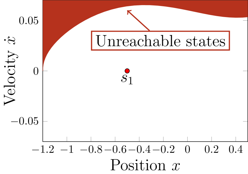
Weakly-communicating MDPs and misspecified states. One of the main limitations of UCRLย [2] and optimistic PSRLย [12] is that they require the MDP to be communicating so that its diameter $D$ (i.e., the length of the longest path among all shortest paths between any pair of states) is finite. While assuming that all states are reachable may seem a reasonable assumption, it is rarely verified in practice. In fact, it requires a designer to carefully define a state space $\mathcal{S}$ that contains all reachable states (otherwise it may not be possible to learn the optimal policy), but it excludes unreachable states (otherwise the resulting MDP would be non-communicating). This requires a considerable amount of prior knowledge about the environment. Consider a problem where we learn from images e.g., the Atari Breakout game [13]. The state space is the set of โ€œplausibleโ€ configurations of the brick wall, ball and paddle positions. The situation in which the wall has an hole in the middle is a valid state (e.g., as an initial state) but it cannot be observed/reached starting from a dense wall (see Fig.ย 1(a)). As such, it should be removed to obtain a โ€œwell-designedโ€ state space. While it may be possible to design a suitable set of โ€œreachableโ€ states that define a communicating MDP, this is often a difficult and tedious task, sometimes even impossible. Now consider a continuous domain e.g., the Mountain Car problem [14]. The state is decribed by the position $x$ and velocity $\dot{x}$ along the $x$-axis. The state space of this domain is usually defined as the cartesian product $[-1.2,0.6]\times[-0.07,0.07]$. Unfortunately, this set contains configurations that are not physically reachable as shown on Fig.ย 1(b). The dynamics of the system is constrained by the evolution equations. Therefore, the car can not go arbitrarily fast. On the leftmost position ($x=-1.2$) the speed $\dot{x}$ cannot exceed 00 due to the fact that such position can be reached only with velocity $\dot{x}\leq 0$. To have a higher velocity, the car would need to acquire momentum from further left (i.e., $x<-1.2$) which is impossible by design ($-1.2$ is the left-boundary of the position domain). The maximal speed reachable for $x>-1.2$ can be attained by applying the maximum acceleration at any time step starting from the state $(x,\dot{x})=(-1.2,0)$. This identifies the curve reported in the Fig.ย 1(b) which denotes the boundary of the unreachable region. Note that other states may not be reachable. Whenever the state space is misspecified or the MDP is weakly communicating (i.e., $D=+\infty$), OFU-based algorithms (e.g., UCRL) optimistically attribute large reward and non-zero probability to reach states that have never been observed, and thus they tend to repeatedly attempt to explore unreachable states. This results in poor performance and linear regret. A first attempt to overcome this major limitation is Regal.Cย [3] (Fruit etย al. [6] recently proposed SCAL, an implementable efficient version of Regal.C), which requires prior knowledge of an upper-bound $H$ to the span (i.e., range) of the optimal bias function $h^{*}$. The optimism of UCRL is then โ€œconstrainedโ€ to policies whose bias has span smaller than $H$. This implicitly โ€œremovesโ€ non-reachable states, whose large optimistic reward would cause the span to become too large. Unfortunately, an accurate knowledge of the bias span may not be easier to obtain than designing a well-specified state space. Bartlett and Tewari [3] proposed an alternative algorithm โ€“ Regal.Dโ€“ that leverages on the doubling trickย [15] to avoid any prior knowledge on the span. Nonetheless, we recently noticed a major flaw in the proof of [3, Theorem 3] that questions the validity of the algorithm (see App.ย A for further details). PS-based algorithms also suffer from similar issues.111We notice that the problem of weakly-communicating MDPs and misspecified states does not hold in the more restrictive setting of finite horizonย [e.g., 8] since exploration is directly tailored to the states that are reachable within the known horizon, or under the assumption of the existence of a recurrent stateย [e.g., 16]. To the best of our knowledge, the only regret guarantees available in the literature for this setting are [17, 18, 19]. However, the counter-example of Osband and Roy [20] seems to invalidate the result of Abbasi-Yadkori and Szepesvรกri [17]. On the other hand, Ouyang etย al. [18] and Theocharous etย al. [19] present PS algorithms with expected Bayesian regret scaling linearly with $H$, where $H$ is an upper-bound on the optimal bias spans of all the MDPs that can be drawn from the prior distribution ([18, Asm. 1] and [19, Sec. 5]). In [18, Remark 1], the authors claim that their algorithm does not require the knowledge of $H$ to derive the regret bound. However, in App.ย B we show on a very simple example that for most continuous prior distributions (e.g., uninformative priors like Dirichlet), it is very likely that $H=+\infty$ implying that the regret bound may not hold (similarly for [19]). As a result, similarly to Regal.C, the prior distribution should contain prior knowledge on the bias span to avoid poor performance.

In this paper, we present TUCRL, an algorithm designed to trade-off exploration and exploitation in weakly-communicating and multi-chain MDPs (e.g., MDPs with misspecified states) without any prior knowledge and under the only assumption that the agent starts from a state in a communicating subset of the MDP (Sec.ย 3). In communicating MDPs, TUCRL eventually (after a finite number of steps) performs as UCRL, thus achieving problem-dependent logarithmic regret. When the true MDP is weakly-communicating, we prove that TUCRL achieves a $\widetilde{O}(\sqrt{T})$ regret that with polynomial dependency on the MDP parameters. We also show that it is not possible to design an algorithm achieving logarithmic regret in weakly-communicating MDPs without having an exponential dependence on the MDP parameters (see Sec.ย 5). TUCRL is the first computationally tractable algorithm in the OFU literature that is able to adapt to the MDP nature without any prior knowledge. The theoretical findings are supported by experiments on several domains (see Sec.ย 4).

2 Preliminaries

We consider a finite weakly-communicating Markov decision process [21, Sec. 8.3] $M=\langle\mathcal{S},\mathcal{A},r,p\rangle$ with a set of states $\mathcal{S}$ and a set of actions ๐’œ=โ‹ƒsโˆˆ๐’ฎ๐’œs๐’œsubscript๐‘ ๐’ฎsubscript๐’œ๐‘ \mathcal{A}=\bigcup_{s\in\mathcal{S}}\mathcal{A}_{s}. Each state-action pair (s,a)โˆˆ๐’ฎร—๐’œs๐‘ ๐‘Ž๐’ฎsubscript๐’œ๐‘ (s,a)\in\mathcal{S}\times\mathcal{A}_{s} is characterized by a reward distribution with mean rโ€‹(s,a)๐‘Ÿ๐‘ ๐‘Žr(s,a) and support in $[0,r_{\max}]$ as well as a transition probability distribution $p(\cdot|s,a)$ over next states. In a weakly-communicating MDP, the state-space $\mathcal{S}$ can be partioned into two subspaces [21, Section 8.3.1]: a communicating set of states (denoted $\mathcal{S}^{\texttt{C}}$ in the rest of the paper) with each state in $S^{\texttt{C}}$ accessible โ€“with non-zero probabilityโ€“ from any other state in $S^{\texttt{C}}$ under some stationary deterministic policy, and a โ€“possibly emptyโ€“ set of states that are transient under all policies (denoted $\mathcal{S}^{\texttt{T}}$). We also denote by $S=|\mathcal{S}|$, $S^{\texttt{C}}=|\mathcal{S}^{\texttt{C}}|$ and A=maxsโˆˆ๐’ฎโก|๐’œs|๐ดsubscript๐‘ ๐’ฎsubscript๐’œ๐‘ A=\max_{s\in\mathcal{S}}|\mathcal{A}_{s}| the number of states and actions, and by $\Gamma^{\texttt{C}}=\max_{s\in\mathcal{S}^{\texttt{C}},a\in\mathcal{A}}\|p(\cdot|s,a)\|_{0}$ the maximum support of all transition probabilities $p(\cdot|s,a)$ with sโˆˆ๐’ฎC๐‘ superscript๐’ฎCs\in\mathcal{S}^{\texttt{C}}. The sets $\mathcal{S}^{\texttt{C}}$ and $\mathcal{S}^{\texttt{T}}$ form a partition of $\mathcal{S}$ i.e., $\mathcal{S}^{\texttt{C}}\cap\mathcal{S}^{\texttt{T}}=\emptyset$ and $\mathcal{S}^{\texttt{C}}\cup\mathcal{S}^{\texttt{T}}=\mathcal{S}$. A deterministic policy $\pi:\mathcal{S}\rightarrow\mathcal{A}$ maps states to actions and it has an associated long-term average reward (or gain) and a bias function defined as

gMฯ€โ€‹(s):=limTโ†’โˆž๐”ผโ€‹[1Tโ€‹โˆ‘t=1Trโ€‹(st,ฯ€โ€‹(st))];hMฯ€โ€‹(s):=Cโ€‹-โ€‹limTโ†’โˆžโ€‹๐”ผโ€‹[โˆ‘t=1T(rโ€‹(st,ฯ€โ€‹(st))โˆ’gMฯ€โ€‹(st))],formulae-sequenceassignsubscriptsuperscript๐‘”๐œ‹๐‘€๐‘ subscriptโ†’๐‘‡๐”ผdelimited-[]1๐‘‡superscriptsubscript๐‘ก1๐‘‡๐‘Ÿsubscript๐‘ ๐‘ก๐œ‹subscript๐‘ ๐‘กassignsubscriptsuperscriptโ„Ž๐œ‹๐‘€๐‘ โ†’๐‘‡๐ถ-๐”ผdelimited-[]superscriptsubscript๐‘ก1๐‘‡๐‘Ÿsubscript๐‘ ๐‘ก๐œ‹subscript๐‘ ๐‘กsuperscriptsubscript๐‘”๐‘€๐œ‹subscript๐‘ ๐‘ก\displaystyle g^{\pi}_{M}(s):=\lim_{T\to\infty}\mathbb{E}\bigg{[}\frac{1}{T}\sum_{t=1}^{T}r\big{(}s_{t},\pi(s_{t})\big{)}\bigg{]};\quad h^{\pi}_{M}(s):=\underset{T\to\infty}{C\text{-}\lim}~{}\mathbb{E}\bigg{[}\sum_{t=1}^{T}\big{(}r(s_{t},\pi(s_{t}))-g_{M}^{\pi}(s_{t})\big{)}\bigg{]},

where the bias hMฯ€โ€‹(s)subscriptsuperscriptโ„Ž๐œ‹๐‘€๐‘ h^{\pi}_{M}(s) measures the expected total difference between the rewards accumulated by $\pi$ starting from s๐‘ s and the stationary reward in Cesaro-limit222For policies whose associated Markov chain is aperiodic, the standard limit exists. (denoted $C\text{-}\lim$). Accordingly, the difference of bias values hMฯ€โ€‹(s)โˆ’hMฯ€โ€‹(sโ€ฒ)subscriptsuperscriptโ„Ž๐œ‹๐‘€๐‘ subscriptsuperscriptโ„Ž๐œ‹๐‘€superscript๐‘ โ€ฒh^{\pi}_{M}(s)-h^{\pi}_{M}(s^{\prime}) quantifies the (dis-)advantage of starting in state s๐‘ s rather than sโ€ฒsuperscript๐‘ โ€ฒs^{\prime}. In the following, we drop the dependency on $M$ whenever clear from the context and denote by sโ€‹p๐’ฎโ€‹{hฯ€}:=maxsโˆˆ๐’ฎโกhฯ€โ€‹(s)โˆ’minsโˆˆ๐’ฎโกhฯ€โ€‹(s)assign๐‘ subscript๐‘๐’ฎsuperscriptโ„Ž๐œ‹subscript๐‘ ๐’ฎsuperscriptโ„Ž๐œ‹๐‘ subscript๐‘ ๐’ฎsuperscriptโ„Ž๐œ‹๐‘ sp_{\mathcal{S}}\left\{{h^{\pi}}\right\}:=\max_{s\in\mathcal{S}}h^{\pi}(s)-\min_{s\in\mathcal{S}}h^{\pi}(s) the span of the bias function. In weakly communicating MDPs, any optimal policy ฯ€โˆ—โˆˆargโกmaxฯ€โกgฯ€โ€‹(s)superscript๐œ‹subscript๐œ‹superscript๐‘”๐œ‹๐‘ \pi^{*}\in\operatorname*{\arg\,\max}_{\pi}g^{\pi}(s) has constant gain, i.e., gฯ€โˆ—โ€‹(s)=gโˆ—superscript๐‘”superscript๐œ‹๐‘ superscript๐‘”g^{\pi^{*}}(s)=g^{*} for all sโˆˆ๐’ฎ๐‘ ๐’ฎs\in\mathcal{S}. Finally, we denote by $D$, resp. $D^{\texttt{C}}$, the diameter of $M$, resp. the diameter of the communicating part of $M$ (i.e., restricted to the set $\mathcal{S}^{\texttt{C}}$):

D:=max(s,sโ€ฒ)โˆˆ๐’ฎร—๐’ฎ,sโ‰ sโ€ฒโก{ฯ„Mโ€‹(sโ†’sโ€ฒ)},DC:=max(s,sโ€ฒ)โˆˆ๐’ฎCร—๐’ฎC,sโ‰ sโ€ฒโก{ฯ„Mโ€‹(sโ†’sโ€ฒ)},formulae-sequenceassign๐ทsubscriptformulae-sequence๐‘ superscript๐‘ โ€ฒ๐’ฎ๐’ฎ๐‘ superscript๐‘ โ€ฒsubscript๐œ๐‘€โ†’๐‘ superscript๐‘ โ€ฒassignsuperscript๐ทCsubscriptformulae-sequence๐‘ superscript๐‘ โ€ฒsuperscript๐’ฎCsuperscript๐’ฎC๐‘ superscript๐‘ โ€ฒsubscript๐œ๐‘€โ†’๐‘ superscript๐‘ โ€ฒ\displaystyle D:=\max_{(s,s^{\prime})\in\mathcal{S}\times\mathcal{S},s\neq s^{\prime}}\{\tau_{M}(s\to s^{\prime})\},\qquad D^{\texttt{C}}:=\max_{(s,s^{\prime})\in\mathcal{S}^{\texttt{C}}\times\mathcal{S}^{\texttt{C}},s\neq s^{\prime}}\{\tau_{M}(s\to s^{\prime})\}, (1)

where ฯ„Mโ€‹(sโ†’sโ€ฒ)subscript๐œ๐‘€โ†’๐‘ superscript๐‘ โ€ฒ\tau_{M}(s\to s^{\prime}) is the expected time of the shortest path from s๐‘ s to sโ€ฒsuperscript๐‘ โ€ฒs^{\prime} in $M$.

Learning problem. Let $M^{*}$ be the true (unknown) weakly-communicating MDP. We consider the learning problem where $\mathcal{S}$, $\mathcal{A}$ and $r_{\max}$ are known, while sets $\mathcal{S}^{\texttt{C}}$ and $\mathcal{S}^{\texttt{T}}$, rewards $r$ and transition probabilities $p$ are unknown and need to be estimated on-line. We evaluate the performance of a learning algorithm $\mathfrak{A}$ after $T$ time steps by its cumulative regret ฮ”โ€‹(๐”„,T)=Tโ€‹gโˆ—โˆ’โˆ‘t=1Trtโ€‹(st,at)ฮ”๐”„๐‘‡๐‘‡superscript๐‘”superscriptsubscript๐‘ก1๐‘‡subscript๐‘Ÿ๐‘กsubscript๐‘ ๐‘กsubscript๐‘Ž๐‘ก\Delta(\mathfrak{A},T)=Tg^{*}-\sum_{t=1}^{T}r_{t}(s_{t},a_{t}). Furthermore, we state the following assumption.

Assumption 1.

The initial state s1subscript๐‘ 1s_{1} belongs to the communicating set of states $\mathcal{S}^{\texttt{C}}$.

While this assumption somehow restricts the scenario we consider, it is fairly common in practice. For example, all the domains that are characterized by the presence of a resetting distribution (e.g., episodic problems) satisfy this assumption (e.g., mountain car, cart pole, Atari games, taxi, etc.).

Multi-chain MDPs. While we consider weakly-communicating MDPs for ease of notation, all our results extend to the more general case of multi-chain MDPs.333In the case of misspecified states, we implicitly define a multi-chain MDP, where each non-reachable state has a self-loop dynamics and it defines a โ€œsingletonโ€ communicating subset. In this case, there may be multiple communicating and transient sets of states and the optimal gain $g^{*}$ is different in each communicating subset. In this case we define $S^{\texttt{C}}$ as the set of states that are accessible โ€“with non-zero probabilityโ€“ from s1subscript๐‘ 1s_{1} (s1subscript๐‘ 1s_{1} included) under some stationary deterministic policy. $\mathcal{S}^{\texttt{T}}$ is defined as the complement of $S^{\texttt{C}}$ in $\mathcal{S}$ i.e., $\mathcal{S}^{\texttt{T}}:=\mathcal{S}\setminus S^{\texttt{C}}$. With these new definitions of $S^{\texttt{C}}$ and $\mathcal{S}^{\texttt{T}}$, Asm.ย 1 needs to be reformulated as follows:

Assumption 1 for Multi-chain MDPs. The initial state s1subscript๐‘ 1s_{1} is accessible โ€“with non-zero probabilityโ€“ from any other state in $\mathcal{S}^{\texttt{C}}$ under some stationary deterministic policy. Equivalently, $\mathcal{S}^{\texttt{C}}$ is a communicating set of states.

Note that the states belonging to $\mathcal{S}^{\texttt{T}}$ can either be transient or belong to other communicating subsets of the MDP disjoint from $\mathcal{S}^{\texttt{C}}$. It does not really matter because the states in $\mathcal{S}^{\texttt{T}}$ will never be visited by definition. As a result, the regret is still defined as before, where the learning performance is compared to the optimal gain gโˆ—โ€‹(s1)superscript๐‘”subscript๐‘ 1g^{*}(s_{1}) related to the communicating set of states ๐’ฎCโˆ‹s1subscript๐‘ 1superscript๐’ฎC\mathcal{S}^{\texttt{C}}\ni s_{1}.

3 Truncated Upper-Confidence for Reinforcement Learning (TUCRL)

In this section we introduce Truncated Upper-Confidence for Reinforcement Learning (TUCRL), an optimistic online RL algorithm that efficiently balances exploration and exploitation to learn in non-communicating MDPs without prior knowledge (Fig.ย 2).

Similar to UCRL, at the beginning of each episode $k$, TUCRL constructs confidence intervals for the reward and the dynamics of the MDP. Formally, for any (s,a)โˆˆ๐’ฎร—๐’œ๐‘ ๐‘Ž๐’ฎ๐’œ(s,a)\in\mathcal{S}\times\mathcal{A} we define

Bp,kโ€‹(s,a)subscript๐ต๐‘๐‘˜๐‘ ๐‘Ž\displaystyle B_{p,k}(s,a) $\displaystyle=\left\{\widetilde{p}(\cdot|s,a)\in\mathcal{C}:~{}\forall s^{\prime}\in\mathcal{S},|\widetilde{p}(s^{\prime}|s,a)-\widehat{p}(s^{\prime}|s,a)|\leq\beta_{p,k}^{sas^{\prime}}\right\},$ (2)
Br,kโ€‹(s,a)subscript๐ต๐‘Ÿ๐‘˜๐‘ ๐‘Ž\displaystyle B_{r,k}(s,a) :=[r^kโ€‹(s,a)โˆ’ฮฒr,ksโ€‹a,r^kโ€‹(s,a)+ฮฒr,ksโ€‹a]โˆฉ[0,rmax],assignabsentsubscript^๐‘Ÿ๐‘˜๐‘ ๐‘Žsuperscriptsubscript๐›ฝ๐‘Ÿ๐‘˜๐‘ ๐‘Žsubscript^๐‘Ÿ๐‘˜๐‘ ๐‘Žsuperscriptsubscript๐›ฝ๐‘Ÿ๐‘˜๐‘ ๐‘Ž0subscript๐‘Ÿ\displaystyle:=[\widehat{r}_{k}(s,a)-\beta_{r,k}^{sa},\widehat{r}_{k}(s,a)+\beta_{r,k}^{sa}]\cap[0,r_{\max}], (3)

where ๐’ž={pโˆˆโ„S|โˆ€sโ€ฒ,pโ€‹(sโ€ฒ)โ‰ฅ0โˆงโˆ‘sโ€ฒpโ€‹(sโ€ฒ)=1}๐’žconditional-set๐‘superscriptโ„๐‘†for-allsuperscript๐‘ โ€ฒ๐‘superscript๐‘ โ€ฒ0subscriptsuperscript๐‘ โ€ฒ๐‘superscript๐‘ โ€ฒ1\mathcal{C}=\{p\in\mathbb{R}^{S}|\forall s^{\prime},~{}p(s^{\prime})\geq 0\wedge\sum_{s^{\prime}}p(s^{\prime})=1\} is the $(S-1)$-probability simplex, while the size of the confidence intervals is constructed using the empirical Bernsteinโ€™s inequalityย [22, 23] as

ฮฒr,ksโ€‹a:=14โ€‹ฯƒ^r,k2โ€‹(s,a)โ€‹bk,ฮดNk+โ€‹(s,a)+493โ€‹rmaxโ€‹bk,ฮดNkยฑโ€‹(s,a),ฮฒp,ksโ€‹aโ€‹sโ€ฒ:=14โ€‹ฯƒ^p,k2โ€‹(sโ€ฒ|s,a)โ€‹bk,ฮดNk+โ€‹(s,a)+493โ€‹bk,ฮดNkยฑโ€‹(s,a),formulae-sequenceassignsuperscriptsubscript๐›ฝ๐‘Ÿ๐‘˜๐‘ ๐‘Ž14superscriptsubscript^๐œŽ๐‘Ÿ๐‘˜2๐‘ ๐‘Žsubscript๐‘๐‘˜๐›ฟsubscriptsuperscript๐‘๐‘˜๐‘ ๐‘Ž493subscript๐‘Ÿsubscript๐‘๐‘˜๐›ฟsubscriptsuperscript๐‘plus-or-minus๐‘˜๐‘ ๐‘Žassignsuperscriptsubscript๐›ฝ๐‘๐‘˜๐‘ ๐‘Žsuperscript๐‘ โ€ฒ14superscriptsubscript^๐œŽ๐‘๐‘˜2conditionalsuperscript๐‘ โ€ฒ๐‘ ๐‘Žsubscript๐‘๐‘˜๐›ฟsubscriptsuperscript๐‘๐‘˜๐‘ ๐‘Ž493subscript๐‘๐‘˜๐›ฟsubscriptsuperscript๐‘plus-or-minus๐‘˜๐‘ ๐‘Ž\displaystyle\beta_{r,k}^{sa}:=\sqrt{\frac{14\widehat{\sigma}_{r,k}^{2}(s,a)b_{k,\delta}}{N^{+}_{k}(s,a)}}+\frac{\frac{49}{3}r_{\max}b_{k,\delta}}{N^{\pm}_{k}(s,a)},\qquad\beta_{p,k}^{sas^{\prime}}:=\sqrt{\frac{14\widehat{\sigma}_{p,k}^{2}(s^{\prime}|s,a)b_{k,\delta}}{N^{+}_{k}(s,a)}}+\frac{\frac{49}{3}b_{k,\delta}}{N^{\pm}_{k}(s,a)},

where Nkโ€‹(s,a)subscript๐‘๐‘˜๐‘ ๐‘ŽN_{k}(s,a) is the number of visits in (s,a)๐‘ ๐‘Ž(s,a) before episode $k$, Nk+โ€‹(s,a):=maxโก{1,Nkโ€‹(s,a)}assignsubscriptsuperscript๐‘๐‘˜๐‘ ๐‘Ž1subscript๐‘๐‘˜๐‘ ๐‘ŽN^{+}_{k}(s,a):=\max\{1,N_{k}(s,a)\}, Nkยฑโ€‹(s,a):=maxโก{1,Nkโ€‹(s,a)โˆ’1}assignsubscriptsuperscript๐‘plus-or-minus๐‘˜๐‘ ๐‘Ž1subscript๐‘๐‘˜๐‘ ๐‘Ž1N^{\pm}_{k}(s,a):=\max\{1,N_{k}(s,a)-1\}, ฯƒ^r,k2โ€‹(s,a)superscriptsubscript^๐œŽ๐‘Ÿ๐‘˜2๐‘ ๐‘Ž\widehat{\sigma}_{r,k}^{2}(s,a) and ฯƒ^p,k2โ€‹(sโ€ฒ|s,a)superscriptsubscript^๐œŽ๐‘๐‘˜2conditionalsuperscript๐‘ โ€ฒ๐‘ ๐‘Ž\widehat{\sigma}_{p,k}^{2}(s^{\prime}|s,a) are the empirical variances of rโ€‹(s,a)๐‘Ÿ๐‘ ๐‘Žr(s,a) and pโ€‹(sโ€ฒ|s,a)๐‘conditionalsuperscript๐‘ โ€ฒ๐‘ ๐‘Ž{p}(s^{\prime}|s,a) and $b_{k,\delta}=\ln(2SAt_{k}/\delta)$. The set of plausible MDPs associated with the confidence intervals is then ${\mathcal{M}}_{k}=\big{\{}M=(\mathcal{S},\mathcal{A},\widetilde{r},\widetilde{p}):\;\widetilde{r}(s,a)\in B_{r,k}(s,a),\;\widetilde{p}(\cdot|s,a)\in B_{p,k}(s,a)\big{\}}$. UCRL is optimistic w.r.t.ย the confidence intervals so that for all states s๐‘ s that have never been visited the optimistic reward r~โ€‹(s,a)~๐‘Ÿ๐‘ ๐‘Ž\widetilde{r}(s,a) is set to $r_{\max}$, while all transitions to s๐‘ s (i.e., p~โ€‹(s|โ‹…,โ‹…)~๐‘conditional๐‘ โ‹…โ‹…\widetilde{p}(s|\cdot,\cdot)) are set to the largest value compatible with $B_{p,k}(\cdot,\cdot)$. Unfortunately, some of the states with Nkโ€‹(s,a)=0subscript๐‘๐‘˜๐‘ ๐‘Ž0N_{k}(s,a)=0 may be actually unreachable (i.e., sโˆˆ๐’ฎT๐‘ superscript๐’ฎTs\in\mathcal{S}^{\texttt{T}}) and UCRL would uniformly explore the policy space with the hope that at least one policy reaches those (optimistically desirable) states. TUCRL addresses this issue by first constructing empirical estimates of $\mathcal{S}^{\texttt{C}}$ and $\mathcal{S}^{\texttt{T}}$ (i.e., the set of communicating and transient states in $M^{*}$) using the states that have been visited so far, that is ๐’ฎkC:={sโˆˆ๐’ฎ|โˆ‘aโˆˆ๐’œsNkโ€‹(s,a)>0}โˆช{stk}assignsubscriptsuperscript๐’ฎC๐‘˜conditional-set๐‘ ๐’ฎsubscript๐‘Žsubscript๐’œ๐‘ subscript๐‘๐‘˜๐‘ ๐‘Ž0subscript๐‘ subscript๐‘ก๐‘˜\mathcal{S}^{\texttt{C}}_{k}:=\left\{s\in\mathcal{S}\;\big{|}\;\sum_{a\in\mathcal{A}_{s}}N_{k}(s,a)>0\right\}\cup\{s_{t_{k}}\} and $\mathcal{S}^{\texttt{T}}_{k}:=\mathcal{S}\setminus\mathcal{S}^{\texttt{C}}_{k}$, where $t_{k}$ is the starting time of episode $k$.

In order to avoid optimistic exploration attempts to unreachable states, we could simply execute UCRL on $\mathcal{S}^{\texttt{C}}_{k}$, which is guaranteed to contain only states in the communicating set (since s1โˆˆ๐’ฎCsubscript๐‘ 1superscript๐’ฎCs_{1}\in\mathcal{S}^{\texttt{C}} by Asm.ย 1, we have that $\mathcal{S}^{\texttt{C}}_{k}\subseteq\mathcal{S}^{\texttt{C}}$). Nonetheless, this algorithm could under-explore state-action pairs that would allow discovering other states in $\mathcal{S}^{\texttt{C}}$, thus getting stuck in a subset of the communicating states of the MDP and suffering linear regret. While the states in $\mathcal{S}^{\texttt{C}}_{k}$ are guaranteed to be in the communicating subset, it is not possible to know whether states in $\mathcal{S}^{\texttt{T}}_{k}$ are actually reachable from $\mathcal{S}^{\texttt{C}}_{k}$ or not. Then TUCRL first โ€œguessesโ€ a lower bound on the probability of transition from states sโˆˆ๐’ฎkC๐‘ subscriptsuperscript๐’ฎC๐‘˜s\in\mathcal{S}^{\texttt{C}}_{k} to sโ€ฒโˆˆ๐’ฎkTsuperscript๐‘ โ€ฒsubscriptsuperscript๐’ฎT๐‘˜s^{\prime}\in\mathcal{S}^{\texttt{T}}_{k} and whenever the maximum transition probability from s๐‘ s to sโ€ฒsuperscript๐‘ โ€ฒs^{\prime} compatible with the confidence intervals (i.e., p^kโ€‹(sโ€ฒ|s,a)+ฮฒp,ksโ€‹aโ€‹sโ€ฒsubscript^๐‘๐‘˜conditionalsuperscript๐‘ โ€ฒ๐‘ ๐‘Žsuperscriptsubscript๐›ฝ๐‘๐‘˜๐‘ ๐‘Žsuperscript๐‘ โ€ฒ\widehat{p}_{k}(s^{\prime}|s,a)+\beta_{p,k}^{sas^{\prime}}) is below the lower bound, it assumes that such transition is not possible. This strategy is based on the intuition that a transition either does not exist or it should have a sufficiently โ€œbigโ€ mass. However, these transitions should be periodically reconsidered in order to avoid under-exploration issues. More formally, let $(\rho_{t})_{t\in\mathbb{N}}$ be a non-increasing sequence to be defined later, for all sโ€ฒโˆˆ๐’ฎkTsuperscript๐‘ โ€ฒsubscriptsuperscript๐’ฎT๐‘˜s^{\prime}\in\mathcal{S}^{\texttt{T}}_{k}, sโˆˆ๐’ฎkC๐‘ subscriptsuperscript๐’ฎC๐‘˜s\in\mathcal{S}^{\texttt{C}}_{k} and aโˆˆ๐’œs๐‘Žsubscript๐’œ๐‘ a\in\mathcal{A}_{s}, the empirical mean p^kโ€‹(sโ€ฒ|s,a)subscript^๐‘๐‘˜conditionalsuperscript๐‘ โ€ฒ๐‘ ๐‘Ž\widehat{p}_{k}(s^{\prime}|s,a) and variance ฯƒ^p,k2โ€‹(sโ€ฒ|s,a)superscriptsubscript^๐œŽ๐‘๐‘˜2conditionalsuperscript๐‘ โ€ฒ๐‘ ๐‘Ž\widehat{\sigma}_{p,k}^{2}(s^{\prime}|s,a) are zero (i.e., this transition has never been observed so far), so the largest probability (most optimistic) of transition from s๐‘ s to sโ€ฒsuperscript๐‘ โ€ฒs^{\prime} through any action $a$ is p~k+โ€‹(sโ€ฒ|s,a)=493โ€‹bk,ฮดNkยฑโ€‹(s,a)superscriptsubscript~๐‘๐‘˜conditionalsuperscript๐‘ โ€ฒ๐‘ ๐‘Ž493subscript๐‘๐‘˜๐›ฟsubscriptsuperscript๐‘plus-or-minus๐‘˜๐‘ ๐‘Ž\widetilde{p}_{k}^{+}(s^{\prime}|s,a)=\frac{49}{3}\frac{b_{k,\delta}}{N^{\pm}_{k}(s,a)}. TUCRL compares p~k+โ€‹(sโ€ฒ|s,a)superscriptsubscript~๐‘๐‘˜conditionalsuperscript๐‘ โ€ฒ๐‘ ๐‘Ž\widetilde{p}_{k}^{+}(s^{\prime}|s,a) to $\rho_{t_{k}}$ and forces all transition probabilities below the threshold to zero, while the confidence intervals of transitions to states that have already been explored (i.e., in $\mathcal{S}^{\texttt{C}}_{k}$) are preserved unchanged. This corresponds to constructing the alternative confidence interval

Bยฏp,kโ€‹(s,a)subscriptยฏ๐ต๐‘๐‘˜๐‘ ๐‘Ž\displaystyle\overline{B}_{p,k}(s,a) $\displaystyle=B_{p,k}(s,a)\cap\left\{\widetilde{p}(\cdot|s,a)\in\mathcal{C}:~{}\forall s^{\prime}\in\mathcal{S}^{\texttt{T}}_{k}\text{ and }\widetilde{p}_{k}^{+}(s^{\prime}|s,a)<\rho_{t_{k}},\widetilde{p}(s^{\prime}|s,a)=0\right\}.$ (4)

Given $\overline{B}_{p,k}$, TUCRL (implicitly) constructs the corresponding set of plausible MDPs $\overline{\mathcal{M}}_{k}$ and then solves the optimistic optimization problem

$$(\widetilde{M}_{k},\widetilde{\pi}_{k})=\operatorname*{\arg\,\max}_{M\in\overline{\mathcal{M}}_{k},\pi}\{g^{\pi}_{M}\}.$$ (5)

The resulting algorithm follows the same structure as UCRL and it is shown in Fig.ย 2. The episode stopping condition at line 4 is slightly modified w.r.t.ย UCRL. In fact, it guarantees that one action is always executed and it forces an episode to terminate as soon as a state previously in $\mathcal{S}^{\texttt{T}}_{k}$ is visited (i.e., Nkโ€‹(st,a)=0subscript๐‘๐‘˜subscript๐‘ ๐‘ก๐‘Ž0N_{k}(s_{t},a)=0). This minor change guarantees that Nk+1โ€‹(s,a)=0subscript๐‘๐‘˜1๐‘ ๐‘Ž0N_{k+1}(s,a)=0 for all the states sโˆˆ๐’ฎkT๐‘ subscriptsuperscript๐’ฎT๐‘˜s\in\mathcal{S}^{\texttt{T}}_{k} that were not reachable at the beginning of the episode. The algorithm also needs minor modifications to the extended value iteration (EVI) algorithm used to solveย (5) to guarantee both efficiency and convergence. All technical details are reported in App.ย C.

Input: Confidence $\delta\in]0,1[$, $r_{\max}$, $\mathcal{S}$, $\mathcal{A}$ Initialization: Set N0โ€‹(s,a):=0assignsubscript๐‘0๐‘ ๐‘Ž0N_{0}(s,a):=0 for any (s,a)โˆˆ๐’ฎร—๐’œ๐‘ ๐‘Ž๐’ฎ๐’œ(s,a)\in\mathcal{S}\times\mathcal{A}, $t:=1$ and observe s1subscript๐‘ 1s_{1}. For episodes $k=1,2,...$ do 1. Set $t_{k}=t$ and episode counters ฮฝkโ€‹(s,a)=0subscript๐œˆ๐‘˜๐‘ ๐‘Ž0\nu_{k}(s,a)=0 2. Compute estimates p^kโ€‹(sโ€ฒ|s,a)subscript^๐‘๐‘˜conditionalsuperscript๐‘ โ€ฒ๐‘ ๐‘Ž\widehat{p}_{k}(s^{\prime}|s,a), r^kโ€‹(s,a)subscript^๐‘Ÿ๐‘˜๐‘ ๐‘Ž\widehat{r}_{k}(s,a) and a set $\overline{\mathcal{M}}_{k}$ 3. Compute an $r_{\max}/\sqrt{t_{k}}$-approximation $\widetilde{\pi}_{k}$ of Eq.ย 5 4. While $t_{k}==t$ or (โˆ‘aโˆˆ๐’œstNkโ€‹(st,a)>0โ€‹ย andย โ€‹ฮฝkโ€‹(st,ฯ€~kโ€‹(st))โ‰คmaxโก{1,Nkโ€‹(st,ฯ€~kโ€‹(st))})subscript๐‘Žsubscript๐’œsubscript๐‘ ๐‘กsubscript๐‘๐‘˜subscript๐‘ ๐‘ก๐‘Ž0ย andย subscript๐œˆ๐‘˜subscript๐‘ ๐‘กsubscript~๐œ‹๐‘˜subscript๐‘ ๐‘ก1subscript๐‘๐‘˜subscript๐‘ ๐‘กsubscript~๐œ‹๐‘˜subscript๐‘ ๐‘ก\Big{(}\sum_{a\in\mathcal{A}_{s_{t}}}N_{k}(s_{t},a)>0\textbf{ and }\nu_{k}(s_{t},\widetilde{\pi}_{k}(s_{t}))\leq\max\left\{1,N_{k}\left(s_{t},\widetilde{\pi}_{k}(s_{t})\right)\right\}\Big{)} do (a) Execute at=ฯ€~kโ€‹(st)subscript๐‘Ž๐‘กsubscript~๐œ‹๐‘˜subscript๐‘ ๐‘กa_{t}=\widetilde{\pi}_{k}(s_{t}), obtain reward $r_{t}$, and observe st+1subscript๐‘ ๐‘ก1s_{t+1} (b) Set $\nu_{k}(s_{t},a_{t})\mathrel{+}=1$ and set $t\mathrel{+}=1$ 5. Set Nk+1โ€‹(s,a)=Nkโ€‹(s,a)+ฮฝkโ€‹(s,a)subscript๐‘๐‘˜1๐‘ ๐‘Žsubscript๐‘๐‘˜๐‘ ๐‘Žsubscript๐œˆ๐‘˜๐‘ ๐‘ŽN_{k+1}(s,a)=N_{k}(s,a)+\nu_{k}(s,a)

Figure 2: TUCRL algorithm.

In practice, we set $\rho_{t}=\frac{49b_{t,\delta}}{3}\sqrt{\frac{SA}{t}}$, so that the condition to remove transition reduces to Nkยฑโ€‹(s,a)>tk/Sโ€‹Asuperscriptsubscript๐‘๐‘˜plus-or-minus๐‘ ๐‘Žsubscript๐‘ก๐‘˜๐‘†๐ดN_{k}^{\pm}(s,a)>\sqrt{\nicefrac{{t_{k}}}{{SA}}}. This shows that only transitions from state-action pairs that have been poorly visited so far are enabled, while if the state-action pair has already been tried often and yet no transition to sโ€ฒโˆˆ๐’ฎkTsuperscript๐‘ โ€ฒsubscriptsuperscript๐’ฎT๐‘˜s^{\prime}\in\mathcal{S}^{\texttt{T}}_{k} is observed, then it is assumed that sโ€ฒsuperscript๐‘ โ€ฒs^{\prime} is not reachable from s,a๐‘ ๐‘Žs,a. When the number of visits in (s,a)๐‘ ๐‘Ž(s,a) is big, the transitions to โ€œunvisitedโ€ states should be discarded because if the transition actually exists, it is most likely extremely small and so it is worth exploring other parts of the MDP first. Symmetrically, when the number of visits in (s,a)๐‘ ๐‘Ž(s,a) is small, the transitions to โ€œunvisitedโ€ states should be enabled because the transitions are quite plausible and the algorithm should try to explore the outcome of taking action $a$ in s๐‘ s and possibly reach states in $\mathcal{S}^{\texttt{T}}_{k}$. We denote the set of state-action pairs that are not sufficiently explored by ๐’ฆk={(s,a)โˆˆ๐’ฎkCร—๐’œ:Nkยฑโ€‹(s,a)โ‰คtk/Sโ€‹A}subscript๐’ฆ๐‘˜conditional-set๐‘ ๐‘Žsubscriptsuperscript๐’ฎC๐‘˜๐’œsuperscriptsubscript๐‘๐‘˜plus-or-minus๐‘ ๐‘Žsubscript๐‘ก๐‘˜๐‘†๐ด\mathcal{K}_{k}=\big{\{}(s,a)\in\mathcal{S}^{\texttt{C}}_{k}\times\mathcal{A}\,:\,N_{k}^{\pm}(s,a)\leq\sqrt{\nicefrac{{t_{k}}}{{SA}}}\big{\}}.

3.1 Analysis of TUCRL

We prove that the regret of TUCRL is bounded as follows.

Theorem 1.

For any weakly communicating MDP $M$, with probability at least $1-\delta$ it holds that for any $T>1$, the regret of TUCRL is bounded as

$$\Delta({\small\textsc{TUCRL}},T)=O\left(r_{\max}D^{\texttt{C}}\sqrt{\Gamma^{\texttt{C}}S^{\texttt{C}}AT\ln\left(\frac{SAT}{\delta}\right)}+r_{\max}\Big{(}D^{\texttt{C}}\Big{)}^{2}S^{3}A\ln^{2}\left(\frac{SAT}{\delta}\right)\right).$$

The first term in the regret shows the ability of TUCRL to adapt to the communicating part of the true MDP $M^{*}$ by scaling with the communicating diameter $D^{\texttt{C}}$ and MDP parameters $S^{\texttt{C}}$ and $\Gamma^{\texttt{C}}$. The second term corresponds to the regret incurred in the early stage where the regret grows linearly. When $M^{*}$ is communicating, we match the square-root term of UCRL (first term), while the second term is bigger than the one appearing in UCRL by a multiplicative factor $D^{\texttt{C}}S$ (ignoring logarithmic terms, see Sec.ย 5).

We now provide a sketch of the proof of Thm.ย 1 (the full proof is reported in App.ย D). In order to preserve readability, all following inequalities should be interpreted up to minor approximations and in high probability.

Let ฮ”k:=โˆ‘s,aฮฝkโ€‹(s,a)โ€‹(gโˆ—โˆ’rโ€‹(s,a))assignsubscriptฮ”๐‘˜subscript๐‘ ๐‘Žsubscript๐œˆ๐‘˜๐‘ ๐‘Žsuperscript๐‘”๐‘Ÿ๐‘ ๐‘Ž\Delta_{k}:=\sum_{s,a}\nu_{k}(s,a)(g^{*}-r(s,a)) be the regret incurred in episode $k$, where ฮฝkโ€‹(s,a)subscript๐œˆ๐‘˜๐‘ ๐‘Ž\nu_{k}(s,a) is the number of visits to s,a๐‘ ๐‘Žs,a in episode $k$. We decompose the regret as

$\displaystyle\Delta({\small\textsc{TUCRL}},T)\lesssim\sum_{k=1}^{m}\Delta_{k}\cdot\mathbbm{1}\{M^{*}\in\mathcal{M}_{k}\}\lesssim\sum_{k=1}^{m}\Delta_{k}\cdot\mathbbm{1}\{t_{k}<C(k)\}+\sum_{k=1}^{m}\Delta_{k}\cdot\mathbbm{1}\{t_{k}\geq C(k)\}$

where $C(k)=O\left((D^{\texttt{C}})^{2}S^{3}A\ln^{2}(\nicefrac{{2SAt_{k}}}{{\delta}})\right)$ defines the length of a full exploratory phase, where the agent may suffer linear regret.

Optimism. The first technical difficulty is that whenever some transitions are disabled, the plausible set of MDPs $\overline{\mathcal{M}}_{k}$ may actually be biased and not contain the true MDP $M^{*}$. This requires to prove that TUCRL (i.e., the gain of the solution returned by EVI) is always optimistic despite โ€œwrongโ€ confidence intervals. The following lemma helps to identify the possible scenarios that TUCRL can produce (see App.ย D.2).444Notice that $M^{*}\in\mathcal{M}_{k}$ is true w.h.p. since $\mathcal{M}_{k}$ is obtained using non-truncated confidence intervals.

Lemma 1.

Let episode $k$ be such that $M^{*}\in\mathcal{M}_{k}$, ๐’ฎkTโ‰ โˆ…subscriptsuperscript๐’ฎT๐‘˜\mathcal{S}^{\texttt{T}}_{k}\neq\emptyset and $t_{k}\geq C(k)$. Then, either $\mathcal{S}^{\texttt{T}}_{k}=\mathcal{S}^{\texttt{T}}$ (case I) or ๐’ฆkโ‰ โˆ…subscript๐’ฆ๐‘˜\mathcal{K}_{k}\neq\emptyset, i.e., โˆƒ(s,a)โˆˆ๐’ฎkCร—๐’œ๐‘ ๐‘Žsubscriptsuperscript๐’ฎC๐‘˜๐’œ\exists(s,a)\in\mathcal{S}^{\texttt{C}}_{k}\times\mathcal{A} for which transitions to $\mathcal{S}^{\texttt{T}}_{k}$ are allowed (case II).

This result basically excludes the case where $\mathcal{S}^{\texttt{T}}_{k}\supset\mathcal{S}^{\texttt{T}}$ (i.e., some states have not been reached) and yet no transition from $\mathcal{S}^{\texttt{C}}_{k}$ to them is enabled. We start noticing that when $\mathcal{S}^{\texttt{T}}_{k}=\emptyset$, the true MDP $M^{*}\in\mathcal{M}_{k}=\overline{\mathcal{M}}_{k}$ w.h.p. by construction of the confidence intervals. Similarly, if $\mathcal{S}^{\texttt{T}}_{k}=\mathcal{S}^{\texttt{T}}$ then $M^{*}\in\overline{\mathcal{M}}_{k}$ w.h.p., since TUCRL only truncates transitions that are indeed forbidden in $M^{*}$ itself. In both cases, we can use the same arguments inย [2] to prove optimism. In case II the gain of any state sโ€ฒโˆˆ๐’ฎkTsuperscript๐‘ โ€ฒsubscriptsuperscript๐’ฎT๐‘˜s^{\prime}\in\mathcal{S}^{\texttt{T}}_{k} is set to $r_{\max}$ and, since there exists a path from $\mathcal{S}^{\texttt{C}}_{k}$ to $\mathcal{S}^{\texttt{T}}_{k}$, the gain of the solution returned by EVI is $r_{\max}$, which makes it trivially optimistic. As a result we can conclude that $\widetilde{g}_{k}\gtrsim g^{*}$ (up to the precision of EVI).

Per-episode regret. After bounding the optimistic reward r~kโ€‹(s,a)subscript~๐‘Ÿ๐‘˜๐‘ ๐‘Ž\widetilde{r}_{k}(s,a) w.r.t.ย rโ€‹(s,a)๐‘Ÿ๐‘ ๐‘Žr(s,a), the only part left to bound the per-episode regret $\Delta_{k}$ is the term ฮ”~k=โˆ‘s,aฮฝkโ€‹(s,a)โ€‹(g~kโˆ’r~kโ€‹(s,a))subscript~ฮ”๐‘˜subscript๐‘ ๐‘Žsubscript๐œˆ๐‘˜๐‘ ๐‘Žsubscript~๐‘”๐‘˜subscript~๐‘Ÿ๐‘˜๐‘ ๐‘Ž\widetilde{\Delta}_{k}=\sum_{s,a}\nu_{k}(s,a)(\widetilde{g}_{k}-\widetilde{r}_{k}(s,a)). Similar to UCRL, we could use the (optimistic) optimality equation and rewrite $\widetilde{\Delta}_{k}$ as

ฮ”~k=โˆ‘sโˆˆ๐’ฎฮฝkโ€‹(s,ฯ€~kโ€‹(s))โ€‹(โˆ‘sโ€ฒโˆˆ๐’ฎp~kโ€‹(sโ€ฒ|s,ฯ€~kโ€‹(s))โ€‹h~kโ€‹(sโ€ฒ)โˆ’h~kโ€‹(s))=ฮฝkโ€ฒโ€‹(P~kโˆ’I)โ€‹wksubscript~ฮ”๐‘˜subscript๐‘ ๐’ฎsubscript๐œˆ๐‘˜๐‘ subscript~๐œ‹๐‘˜๐‘ subscriptsuperscript๐‘ โ€ฒ๐’ฎsubscript~๐‘๐‘˜conditionalsuperscript๐‘ โ€ฒ๐‘ subscript~๐œ‹๐‘˜๐‘ subscript~โ„Ž๐‘˜superscript๐‘ โ€ฒsubscript~โ„Ž๐‘˜๐‘ superscriptsubscript๐œˆ๐‘˜โ€ฒsubscript~๐‘ƒ๐‘˜๐ผsubscript๐‘ค๐‘˜\displaystyle\begin{split}\widetilde{\Delta}_{k}=\sum_{s\in{\color[rgb]{1,0,0}\definecolor[named]{pgfstrokecolor}{rgb}{1,0,0}\mathcal{S}}}\nu_{k}(s,\widetilde{\pi}_{k}(s))\bigg{(}\sum_{s^{\prime}\in{\color[rgb]{1,0,0}\definecolor[named]{pgfstrokecolor}{rgb}{1,0,0}\mathcal{S}}}\widetilde{p}_{k}(s^{\prime}|s,\widetilde{\pi}_{k}(s))\widetilde{h}_{k}(s^{\prime})-\widetilde{h}_{k}(s)\bigg{)}=\nu_{k}^{\prime}\left(\widetilde{P}_{k}-I\right)w_{k}\end{split} (6)

where wk:=h~kโˆ’minsโˆˆ๐’ฎโก{h~k}โ€‹eassignsubscript๐‘ค๐‘˜subscript~โ„Ž๐‘˜subscript๐‘ ๐’ฎsubscript~โ„Ž๐‘˜๐‘’w_{k}:=\widetilde{h}_{k}-\min_{s\in\mathcal{S}}\{\widetilde{h}_{k}\}e is a shifted version of the vector $\widetilde{h}_{k}$ returned by EVI at episode $k$, and then proceed by bounding the difference between $\widetilde{P}_{k}$ and $P_{k}$ using standard concentration inequalities. Nonetheless, we would be left with the problem of bounding the $\ell_{\infty}$ norm of $w_{k}$ (i.e., the range of the optimistic vector $\widetilde{h}_{k}$) over the whole state space, i.e., โ€–wkโ€–โˆž=sโ€‹p๐’ฎโ€‹{h~k}=maxsโˆˆ๐’ฎโกh~kโ€‹(s)โˆ’minsโˆˆ๐’ฎโกh~kโ€‹(s)subscriptnormsubscript๐‘ค๐‘˜๐‘ subscript๐‘๐’ฎsubscript~โ„Ž๐‘˜subscript๐‘ ๐’ฎsubscript~โ„Ž๐‘˜๐‘ subscript๐‘ ๐’ฎsubscript~โ„Ž๐‘˜๐‘ \|w_{k}\|_{\infty}=sp_{\mathcal{S}}\{\widetilde{h}_{k}\}=\max_{s\in\mathcal{S}}\widetilde{h}_{k}(s)-\min_{s\in\mathcal{S}}\widetilde{h}_{k}(s). While in communicating MDPs, it is possible to bound this quantity by the diameter of the MDP as sโ€‹p๐’ฎโ€‹{hk}โ‰คD๐‘ subscript๐‘๐’ฎsubscriptโ„Ž๐‘˜๐ทsp_{\mathcal{S}}\left\{{h_{k}}\right\}\leq Dย [2, Sec. 4.3], in weakly-communicating MDPs $D=+\infty$, thus making this result uninformative. As a result, we need to restrict our attention to the subset of communicating states $\mathcal{S}^{\texttt{C}}$, where the diameter is finite. We then split the per-step regret over states depending on whether they are explored enough or not as ฮ”kโ‰ฒโˆ‘s,aฮฝkโ€‹(s,a)โ€‹(g~kโˆ’r~kโ€‹(s,a))โ€‹๐Ÿ™โ€‹{(s,a)โˆ‰๐’ฆk}+rmaxโ€‹โˆ‘s,aฮฝkโ€‹(s,a)โ€‹๐Ÿ™โ€‹{(s,a)โˆˆ๐’ฆk}less-than-or-similar-tosubscriptฮ”๐‘˜subscript๐‘ ๐‘Žsubscript๐œˆ๐‘˜๐‘ ๐‘Žsubscript~๐‘”๐‘˜subscript~๐‘Ÿ๐‘˜๐‘ ๐‘Ž1๐‘ ๐‘Žsubscript๐’ฆ๐‘˜subscript๐‘Ÿsubscript๐‘ ๐‘Žsubscript๐œˆ๐‘˜๐‘ ๐‘Ž1๐‘ ๐‘Žsubscript๐’ฆ๐‘˜\Delta_{k}\lesssim\sum_{s,a}\nu_{k}(s,a)(\widetilde{g}_{k}-\widetilde{r}_{k}(s,a))\mathbbm{1}\{(s,a)\notin\mathcal{K}_{k}\}+r_{\max}\sum_{s,a}\nu_{k}(s,a)\mathbbm{1}\{(s,a)\in\mathcal{K}_{k}\}. We start focusing on the poorly visited state-action pairs, i.e., (s,a)โˆˆ๐’ฆk๐‘ ๐‘Žsubscript๐’ฆ๐‘˜(s,a)\in\mathcal{K}_{k}. In this case TUCRL may suffer the maximum per-step regret $r_{\max}$ but the number of times this event happen is cumulatively โ€œsmallโ€ (App.ย D.4.1):

Lemma 2.

For any $T\geq 1$ and any sequence of states and actions {s1,a1,โ€ฆโ€‹โ€ฆโ€‹sT,aT}subscript๐‘ 1subscript๐‘Ž1โ€ฆโ€ฆsubscript๐‘ ๐‘‡subscript๐‘Ž๐‘‡\{s_{1},a_{1},\dots\dots s_{T},a_{T}\} we have:

โˆ‘k=1mโˆ‘s,aฮฝkโ€‹(s,a)โ€‹๐Ÿ™โ€‹{Nkยฑโ€‹(s,a)โ‰คtk/Sโ€‹AโŸ(s,a)โˆˆ๐’ฆk}โ‰คโˆ‘t=1T๐Ÿ™โ€‹{Nktยฑโ€‹(st,at)โ‰คt/Sโ€‹A}โ‰ค2โ€‹(SCโ€‹Aโ€‹T+SCโ€‹A)superscriptsubscript๐‘˜1๐‘šsubscript๐‘ ๐‘Žsubscript๐œˆ๐‘˜๐‘ ๐‘Ž1subscriptโŸsuperscriptsubscript๐‘๐‘˜plus-or-minus๐‘ ๐‘Žsubscript๐‘ก๐‘˜๐‘†๐ด๐‘ ๐‘Žsubscript๐’ฆ๐‘˜superscriptsubscript๐‘ก1๐‘‡1superscriptsubscript๐‘subscript๐‘˜๐‘กplus-or-minussubscript๐‘ ๐‘กsubscript๐‘Ž๐‘ก๐‘ก๐‘†๐ด2superscript๐‘†C๐ด๐‘‡superscript๐‘†C๐ด\sum_{k=1}^{m}\sum_{s,a}\nu_{k}(s,a)\mathbbm{1}\{\underbrace{N_{k}^{\pm}(s,a)\leq\sqrt{\nicefrac{{t_{k}}}{{SA}}}}_{(s,a)\in\mathcal{K}_{k}}\}\leq\sum_{t=1}^{T}\mathbbm{1}\left\{N_{k_{t}}^{\pm}(s_{t},a_{t})\leq\sqrt{\nicefrac{{t}}{{SA}}}\right\}\leq 2\left(\sqrt{S^{\texttt{C}}AT}+S^{\texttt{C}}A\right)

When (s,a)โˆ‰๐’ฆk๐‘ ๐‘Žsubscript๐’ฆ๐‘˜(s,a)\notin\mathcal{K}_{k} (i.e., Nkยฑโ€‹(s,a)>tk/Sโ€‹Asuperscriptsubscript๐‘๐‘˜plus-or-minus๐‘ ๐‘Žsubscript๐‘ก๐‘˜๐‘†๐ดN_{k}^{\pm}(s,a)>\sqrt{\nicefrac{{t_{k}}}{{SA}}} holds), โˆ‘s,aฮฝkโ€‹(s,a)โ€‹(g~kโˆ’r~kโ€‹(s,a))โ‹…๐Ÿ™โ€‹{(s,a)โˆ‰๐’ฆk}subscript๐‘ ๐‘Žโ‹…subscript๐œˆ๐‘˜๐‘ ๐‘Žsubscript~๐‘”๐‘˜subscript~๐‘Ÿ๐‘˜๐‘ ๐‘Ž1๐‘ ๐‘Žsubscript๐’ฆ๐‘˜\sum_{s,a}\nu_{k}(s,a)(\widetilde{g}_{k}-\widetilde{r}_{k}(s,a))\cdot\mathbbm{1}\{(s,a)\notin\mathcal{K}_{k}\} can be bounded as in Eq.ย 6 but now restricted on $\mathcal{S}^{\texttt{C}}_{k}$, so that,

$\displaystyle\nu_{k}(\widetilde{P}_{k}-I)\widetilde{h}_{k}$ =โˆ‘sโˆˆ๐’ฎkCฮฝkโ€‹(s,ฯ€~kโ€‹(s))โ€‹(โˆ‘sโ€ฒโˆˆ๐’ฎkCp~kโ€‹(sโ€ฒ|s,ฯ€~kโ€‹(s))โ€‹wkโ€‹(sโ€ฒ)โˆ’wkโ€‹(s)).absentsubscript๐‘ subscriptsuperscript๐’ฎC๐‘˜subscript๐œˆ๐‘˜๐‘ subscript~๐œ‹๐‘˜๐‘ subscriptsuperscript๐‘ โ€ฒsubscriptsuperscript๐’ฎC๐‘˜subscript~๐‘๐‘˜conditionalsuperscript๐‘ โ€ฒ๐‘ subscript~๐œ‹๐‘˜๐‘ subscript๐‘ค๐‘˜superscript๐‘ โ€ฒsubscript๐‘ค๐‘˜๐‘ \displaystyle=\sum_{s\in{\color[rgb]{0,0,1}\definecolor[named]{pgfstrokecolor}{rgb}{0,0,1}\mathcal{S}^{\texttt{C}}_{k}}}\nu_{k}(s,\widetilde{\pi}_{k}(s))\bigg{(}\sum_{s^{\prime}\in{\color[rgb]{0,0,1}\definecolor[named]{pgfstrokecolor}{rgb}{0,0,1}\mathcal{S}^{\texttt{C}}_{k}}}\widetilde{p}_{k}(s^{\prime}|s,\widetilde{\pi}_{k}(s))w_{k}(s^{\prime})-w_{k}(s)\bigg{)}.

Since the stopping condition guarantees that ฮฝkโ€‹(s,ฯ€~kโ€‹(s))=0subscript๐œˆ๐‘˜๐‘ subscript~๐œ‹๐‘˜๐‘ 0\nu_{k}(s,\widetilde{\pi}_{k}(s))=0 for all sโˆˆ๐’ฎkT๐‘ subscriptsuperscript๐’ฎT๐‘˜s\in\mathcal{S}^{\texttt{T}}_{k}, we can first restrict the outer summation to states in $\mathcal{S}^{\texttt{C}}$. Furthermore, all state-action pairs (s,a)โˆ‰๐’ฆk๐‘ ๐‘Žsubscript๐’ฆ๐‘˜(s,a)\notin\mathcal{K}_{k} are such that the optimistic transition probability p~kโ€‹(sโ€ฒ|s,a)subscript~๐‘๐‘˜conditionalsuperscript๐‘ โ€ฒ๐‘ ๐‘Ž\widetilde{p}_{k}(s^{\prime}|s,a) is forced to zero for all sโ€ฒโˆˆ๐’ฎkTsuperscript๐‘ โ€ฒsubscriptsuperscript๐’ฎT๐‘˜s^{\prime}\in\mathcal{S}^{\texttt{T}}_{k}, thus reducing the inner summation. We are then left with providing a bound for the range of $w_{k}$ restricted to the states in $\mathcal{S}^{\texttt{C}}_{k}$, i.e., sโ€‹p๐’ฎkCโ€‹{wk}=maxsโˆˆ๐’ฎkCโก{wk}๐‘ subscript๐‘subscriptsuperscript๐’ฎC๐‘˜subscript๐‘ค๐‘˜subscript๐‘ subscriptsuperscript๐’ฎC๐‘˜subscript๐‘ค๐‘˜sp_{\mathcal{S}^{\texttt{C}}_{k}}\{w_{k}\}=\max_{s\in\mathcal{S}^{\texttt{C}}_{k}}\{w_{k}\}. We recall that EVI run on a set of plausible MDPs $\overline{\mathcal{M}}_{k}$ returns a function $\widetilde{h}_{k}$ such that h~kโ€‹(sโ€ฒ)โˆ’h~kโ€‹(s)โ‰คrmaxโ‹…ฯ„โ„ณยฏkโ€‹(sโ†’sโ€ฒ)subscript~โ„Ž๐‘˜superscript๐‘ โ€ฒsubscript~โ„Ž๐‘˜๐‘ โ‹…subscript๐‘Ÿsubscript๐œsubscriptยฏโ„ณ๐‘˜โ†’๐‘ superscript๐‘ โ€ฒ\widetilde{h}_{k}(s^{\prime})-\widetilde{h}_{k}(s)\leq r_{\max}\cdot\tau_{\overline{\mathcal{M}}_{k}}(s\to s^{\prime}), for any pair s,sโ€ฒโˆˆ๐’ฎ๐‘ superscript๐‘ โ€ฒ๐’ฎs,s^{\prime}\in\mathcal{S}, where ฯ„โ„ณยฏkโ€‹(sโ†’sโ€ฒ)subscript๐œsubscriptยฏโ„ณ๐‘˜โ†’๐‘ superscript๐‘ โ€ฒ\tau_{\overline{\mathcal{M}}_{k}}(s\to s^{\prime}) is the expected shortest path in the extended MDP $\overline{\mathcal{M}}_{k}$. Furthermore, since $M^{*}\in\mathcal{M}_{k}$, for all s,sโ€ฒโˆˆ๐’ฎkC๐‘ superscript๐‘ โ€ฒsubscriptsuperscript๐’ฎC๐‘˜s,s^{\prime}\in\mathcal{S}^{\texttt{C}}_{k}, ฯ„โ„ณkโ€‹(sโ†’sโ€ฒ)โ‰คDCsubscript๐œsubscriptโ„ณ๐‘˜โ†’๐‘ superscript๐‘ โ€ฒsuperscript๐ทC\tau_{\mathcal{M}_{k}}(s\to s^{\prime})\leq D^{\texttt{C}}. Unfortunately, since $M^{*}$ may not belong to $\overline{\mathcal{M}}_{k}$, the bound on the shortest path in $\mathcal{M}_{k}$ (i.e., ฯ„โ„ณkโ€‹(sโ†’sโ€ฒ)subscript๐œsubscriptโ„ณ๐‘˜โ†’๐‘ superscript๐‘ โ€ฒ\tau_{\mathcal{M}_{k}}(s\to s^{\prime})) may not directly translate into a bound for the shortest path in $\overline{\mathcal{M}}_{k}$, thus preventing from bounding the range of $\widetilde{h}_{k}$ even on the subset of states in $\mathcal{S}^{\texttt{C}}_{k}$. Nonetheless, in App.ย E we show that a minor modification to the confidence intervals of $\overline{\mathcal{M}}_{k}$ makes the shortest paths between any two states s,sโ€ฒโˆˆ๐’ฎkC๐‘ superscript๐‘ โ€ฒsubscriptsuperscript๐’ฎC๐‘˜s,s^{\prime}\in\mathcal{S}^{\texttt{C}}_{k} equivalent in both sets of plausible MDPs, thus providing the bound sโ€‹p๐’ฎkCโ€‹{wk}โ‰คDC๐‘ subscript๐‘subscriptsuperscript๐’ฎC๐‘˜subscript๐‘ค๐‘˜superscript๐ทCsp_{\mathcal{S}^{\texttt{C}}_{k}}\{w_{k}\}\leq D^{\texttt{C}}. 555Note that there is not a single way to modify the confidence intervals of $\overline{\mathcal{M}}_{k}$ to keep sโ€‹p๐’ฎkCโ€‹{wk}๐‘ subscript๐‘subscriptsuperscript๐’ฎC๐‘˜subscript๐‘ค๐‘˜sp_{\mathcal{S}^{\texttt{C}}_{k}}\{w_{k}\} under control. In App.ย F we present an alternative modifications for which the shortest paths between any two states s,sโ€ฒโˆˆ๐’ฎkC๐‘ superscript๐‘ โ€ฒsubscriptsuperscript๐’ฎC๐‘˜s,s^{\prime}\in\mathcal{S}^{\texttt{C}}_{k} is not equal but smaller than in $\overline{\mathcal{M}}_{k}$ thus ensuring that sโ€‹p๐’ฎkCโ€‹{wk}โ‰คDC๐‘ subscript๐‘subscriptsuperscript๐’ฎC๐‘˜subscript๐‘ค๐‘˜superscript๐ทCsp_{\mathcal{S}^{\texttt{C}}_{k}}\{w_{k}\}\leq D^{\texttt{C}}. The final regret in Thm.ย 1 is then obtained by combining all different terms.

4 Experiments

Refer to caption Refer to caption
Refer to caption
Figure 3: Cumulative regret in the taxi with misspecified states (left-top) and in the communicating taxi (left-bottom), and in the weakly communicating three-states domain with $D=+\infty$ (right). Confidence intervals $\beta_{r,k}$ and $\beta_{p,k}$ are shrunk by a factor $0.05$ and $0.01$ for the three-states domain and taxi, respectively. Results are averaged over $20$ runs and 95% confidence intervals are reported.

In this section, we present experiments to validate the theoretical findings of Sec.ย 3. We compare TUCRL against UCRL and SCAL.666To the best of out knowledge, there exists no implementable algorithm to solve the optimization step of Regal and Regal.D. We first consider the taxi problemย [24] implemented in OpenAI Gymย [25].777The code is available on GitHub. Even such a simple domain contains misspecified states, since the state space is constructed as the outer product of the taxi position, the passenger position and the destination. This leads to states that cannot be reached from any possible starting configuration (all the starting states belong to $\mathcal{S}^{\texttt{C}}$). More precisely, out of $500$ states in $\mathcal{S}$, $100$ are non-reachable. On Fig.ย 3(left) we compare the regret of UCRL, SCAL and TUCRL when the misspecified states are present (top) and when they are removed (bottom). In the presence of misspecified states (top), the regret of UCRL clearly grows linearly with $T$ while TUCRL is able to learn as expected. On the other hand, when the MDP is communicating (bottom) TUCRL performs similarly to UCRL. The small loss in performance is most likely due to the initial exploration phase during which the confidence intervals on the transition probabilities used by UCRL (see definition of $\overline{\mathcal{M}}_{k}$) are tighter than those used by TUCRL (see definition of $\overline{\mathcal{M}}_{k}^{+}$). TUCRL uses a โ€œlooseโ€ bound on the $\ell_{1}$-norm while UCRL uses $S$ different bounds, one for every possible next state. Finally, SCAL outperforms TUCRL by exploiting prior knowledge on the bias span.

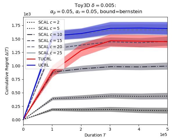
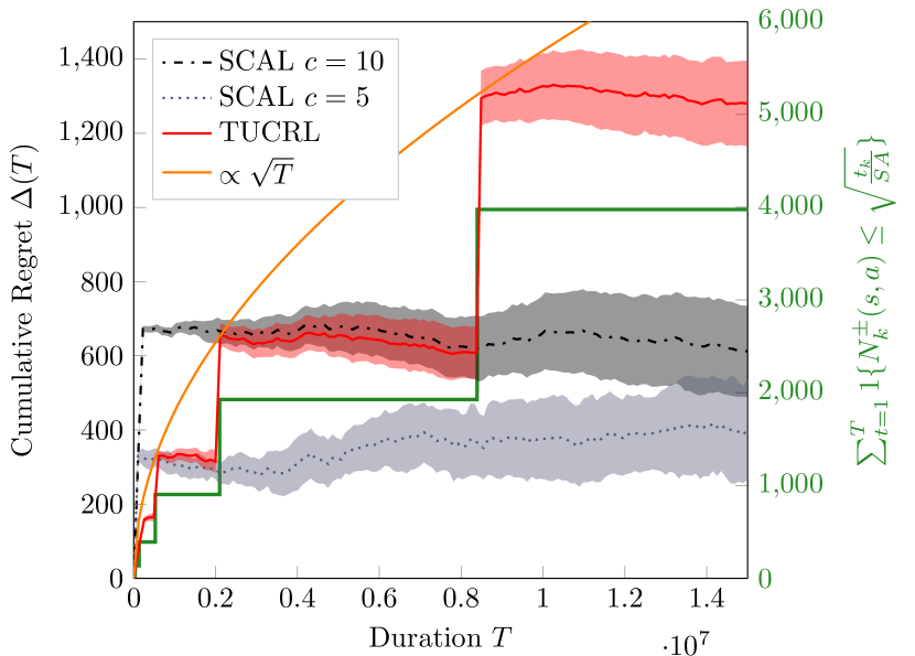
We further study TUCRL regret in the simple three-state domain introduced inย [6] (see App.ย H for details) with different reward distributions (uniform instead of Bernouilli). The environment is composed of only three states (s0subscript๐‘ 0s_{0}, s1subscript๐‘ 1s_{1} and s2subscript๐‘ 2s_{2}) and one action per state, except in s2subscript๐‘ 2s_{2} where two actions are available. As a result, the agent only has the choice between two possible policies. Fig.ย 3(left) shows the cumulative regret achieved by TUCRL and SCAL (with different upper-bounds on the bias span) when the diameter is infinite i.e., ๐’ฎC={s0,s2}superscript๐’ฎCsubscript๐‘ 0subscript๐‘ 2\mathcal{S}^{\texttt{C}}=\{s_{0},s_{2}\} and ๐’ฎT={s1}superscript๐’ฎTsubscript๐‘ 1\mathcal{S}^{\texttt{T}}=\{s_{1}\} (we omit UCRL, since it suffers linear regret). Both SCAL and TUCRL quickly achieve sub-linear regret as predicted by theory. However, SCAL and TUCRL seem to achieve different growth rates in regret: while SCAL appears to reach a logarithmic growth, the regret of TUCRL seems to grow as $\sqrt{T}$ with periodic โ€œjumpsโ€ that are increasingly distant (in time) from each other. This can be explained by the way the algorithm works: while most of the time TUCRL is optimistic on the restricted state space $\mathcal{S}^{\texttt{C}}$ (i.e., $\mathcal{S}^{\texttt{C}}_{k}=\mathcal{S}^{\texttt{C}}$), it periodically allows transitions to the set $\mathcal{S}^{\texttt{T}}$ (i.e., $\mathcal{S}^{\texttt{C}}_{k}=\mathcal{S}$), which is indeed not reachable. Enabling these transitions triggers aggressive exploration during an entire episode. The policy played is then sub-optimal creating a โ€œjumpโ€ in the regret. At the end of this exploratory episode, $\mathcal{S}^{\texttt{C}}_{k}$ will be set again to $\mathcal{S}^{\texttt{C}}$ and the regret will stop increasing until the condition $N_{k}^{\pm}\leq\sqrt{\nicefrac{{t_{k}}}{{SA}}}$ occurs again (the time between two consecutive exploratory episodes grows quadratically). The cumulative regret incurred during exploratory episodes can be bounded by the term plotted in green on Fig.ย 3(left). In Lem.ย 2 we proved that this term is always bounded by $O(\sqrt{S^{\texttt{C}}AT})$. Therefore, it is not surprising to observe a $\sqrt{T}$ increase of both the green and red curves. Unfortunately, the growth rate of the regret will keep increasing as $\sqrt{T}$ and will never become logarithmic unlike SCAL (or UCRL when the MDP is communicating). This is because the condition $N_{k}^{\pm}\leq\sqrt{\nicefrac{{t_{k}}}{{SA}}}$ will always be triggered $\Theta(\sqrt{T})$ times for any $T$. In Sec.ย 5 we show that this is not just a drawback specific to TUCRL, but it is rather an intrinsic limitation of learning in weakly-communicating MDPs.

5 Exploration-exploitation dilemma with infinite diameter

$T$ $\mathbb{E}[\Delta(\textsc{UCRL},T,M)]$ $O(T)$ $O(DS\sqrt{AT\ln(T)})$ $O\left(\frac{D^{2}S^{2}A}{\gamma}\ln(T)\right)$00TMโ€ superscriptsubscript๐‘‡๐‘€โ€ {T}_{M}^{\dagger}${T}_{M}^{*}$Regret upper-bound
(a)
$x$ $y$ $b$ $d$ $\varepsilon$ $1-\varepsilon$ $d$ $b$ $r=0$ $r=\nicefrac{{1}}{{2}}$ $r=0$ $r=1$
(b)
$x$ $y$ $b$ $d$ $b$ $d$ $r=0$ $r=\nicefrac{{1}}{{2}}$ $r=1$ $r=0$
(c)
Figure 4: 4(a) Expected regret of UCRL (with known horizon $T$ given as input) as a function of $T$. 4(c)ย 4(c) Toy example illustrating the difficulty of learning non-communicating MDPs. We represent a family of possible MDPs $\mathcal{M}=(M_{\varepsilon})_{\varepsilon\in[0,1]}$ where the probability $\varepsilon$ to go from $x$ to $y$ lies in $[0,1]$.

In this section we further investigate the empirical difference between SCAL and TUCRL and prove an impossibility result characterising the exploration-exploitation dilemma when the diameter is allowed to be infinite and no prior knowledge on the optimal bias span is available.

We first recall that the expected regret $\mathbbm{E}[\Delta({\small\textsc{UCRL}},M,T)]$ of UCRL (with input parameter $\delta=1/3T$) after $T\geq 1$ time steps and for any finite MDP $M$ can be bounded in several ways:

๐”ผโ€‹[ฮ”โ€‹(UCRL,M,T)]โ‰ค{rmaxโ€‹Tโ€‹(by definition)C1โ‹…rmaxโ€‹Dโ€‹ฮ“โ€‹Sโ€‹Aโ€‹Tโ€‹lnโก(3โ€‹T2)+13โ€‹[2, Theorem 2]C2โ‹…rmaxโ€‹D2โ€‹ฮ“โ€‹Sโ€‹Aฮณโ€‹lnโก(T)+C3โ€‹(M)โ€‹[2, Theorem 4]๐”ผdelimited-[]ฮ”UCRL๐‘€๐‘‡casessubscript๐‘Ÿ๐‘‡(by definition)otherwiseโ‹…subscript๐ถ1subscript๐‘Ÿ๐ทฮ“๐‘†๐ด๐‘‡3superscript๐‘‡213[2, Theorem 2]otherwiseโ‹…subscript๐ถ2subscript๐‘Ÿsuperscript๐ท2ฮ“๐‘†๐ด๐›พ๐‘‡subscript๐ถ3๐‘€[2, Theorem 4]otherwise\displaystyle\mathbbm{E}[\Delta({\small\textsc{UCRL}},M,T)]\leq\begin{cases}r_{\max}T~{}~{}\text{(by definition)}\\ C_{1}\cdot r_{\max}D\sqrt{\Gamma SAT\ln(3T^{2})}+\frac{1}{3}~{}\text{\cite[citep]{[\@@bibref{Number}{Jaksch10}{}{}, Theorem 2]}}\\ C_{2}\cdot r_{\max}\frac{D^{2}\Gamma SA}{\gamma}\ln(T)+C_{3}(M)~{}\text{\cite[citep]{[\@@bibref{Number}{Jaksch10}{}{}, Theorem 4]}}\end{cases} (7)

where ฮณ=gMโˆ—โˆ’maxs,ฯ€โก{gMฯ€โ€‹(s):gMฯ€โ€‹(s)<gMโˆ—}๐›พsubscriptsuperscript๐‘”๐‘€subscript๐‘ ๐œ‹:subscriptsuperscript๐‘”๐œ‹๐‘€๐‘ subscriptsuperscript๐‘”๐œ‹๐‘€๐‘ subscriptsuperscript๐‘”๐‘€\gamma=g^{*}_{M}-\max_{s,\pi}\{g^{\pi}_{M}(s):~{}g^{\pi}_{M}(s)<g^{*}_{M}\} is the gap in gain, $C_{1}:=34$ and $C_{2}:=34^{2}$ are numerical constants independent of $M$, and C3โ€‹(M):=Oโ€‹(maxฯ€:ฯ€โ€‹(s)=aโกTฯ€)assignsubscript๐ถ3๐‘€๐‘‚subscript:๐œ‹๐œ‹๐‘ ๐‘Žsubscript๐‘‡๐œ‹C_{3}(M):=O(\max_{\pi:\pi(s)=a}T_{\pi}) with $T_{\pi}$ a measure of the โ€œmixing timeโ€ of policy $\pi$. The three different bounds lead to three different growth rates for the function $T\longmapsto\mathbbm{E}[\Delta({\small\textsc{UCRL}},M,T)]$ (see Fig.ย 4(a)): 1) for TMโ€ โ‰ฅTโ‰ฅ0superscriptsubscript๐‘‡๐‘€โ€ ๐‘‡0{T}_{M}^{\dagger}\geq T\geq 0, the expected regret is linear in $T$, 2) for TMโˆ—โ‰ฅTโ‰ฅTMโ€ superscriptsubscript๐‘‡๐‘€๐‘‡superscriptsubscript๐‘‡๐‘€โ€ {T}_{M}^{*}\geq T\geq{T}_{M}^{\dagger} the expected regret grows as $\sqrt{T}$, 3) finally for $T\geq{T}_{M}^{*}$, the increase in regret is only logarithmic in $T$. These different โ€œregimesโ€ can be observed empirically (seeย [6, Fig. 5, 12]). Using ย (7), it is easy to show that the time it takes for UCRL to achieve sub-linear regret is at most TMโ€ =O~โ€‹(D2โ€‹ฮ“โ€‹Sโ€‹A)superscriptsubscript๐‘‡๐‘€โ€ ~๐‘‚superscript๐ท2ฮ“๐‘†๐ด{T}_{M}^{\dagger}=\widetilde{O}(D^{2}\Gamma SA). We say that an algorithm is efficient when it achieves sublinear regret after a number of steps that is polynomial in the parameters of the MDP (i.e., UCRL is then efficient). We now show with an example that without prior knowledge, any efficient learning algorithm must satisfy ${T}_{M}^{*}=+\infty$ when $M$ has infinite diameter (i.e., it cannot achieve logarithmic regret).

Example 1.

We consider a family of weakly-communicating MDPs $\mathcal{M}=(M_{\varepsilon})_{\varepsilon\in[0,1]}$ represented on Fig.ย 4(right). Every MDP instance in $\mathcal{M}$ is characterised by a specific value of $\varepsilon\in[0,1]$ which corresponds to the probability to go from $x$ to $y$. For $\varepsilon>0$ (Fig.ย 4(c)), the optimal policy of $M_{\varepsilon}$ is such that $\pi^{*}(x)=b$ and the optimal gain is $g^{*}_{\varepsilon}=1$ while for $\varepsilon=0$ (Fig.ย 4(c)) the optimal policy is such that $\pi^{*}(x)=d$ and the optimal gain is $g^{*}_{0}=1/2$. We assume that the learning agent knows that the true MDP $M^{*}$ belongs to $\mathcal{M}$ but does not know the value $\varepsilon^{*}$ associated to $M^{*}=M_{\varepsilon^{*}}$. We assume that all rewards are deterministic and that the agent starts in state $x$ (coloured in grey).

Lemma 3.

Let $C_{1},C_{2},\alpha,\beta>0$ be positive real numbers and $f$ a function defined for all $\varepsilon\in]0,1]$ by $f(\varepsilon)=C_{1}(1/\varepsilon)^{\alpha}$. There exists no learning algorithm $\mathfrak{A}_{T}$ (with known horizon $T$) satisfying both

  1. 1.

    for all $\varepsilon\in]0,1]$, there exists Tฮตโ€ โ‰คfโ€‹(ฮต)superscriptsubscript๐‘‡๐œ€โ€ ๐‘“๐œ€{T}_{\varepsilon}^{\dagger}\leq f(\varepsilon) such that $\mathbbm{E}[\Delta(\mathfrak{A}_{T},M_{\varepsilon},x,T)]<1/6\cdot T$ for all Tโ‰ฅTฮตโ€ ๐‘‡superscriptsubscript๐‘‡๐œ€โ€ T\geq{T}_{\varepsilon}^{\dagger},

  2. 2.

    and there exists ${T}_{0}^{*}<+\infty$ such that $\mathbbm{E}[\Delta(\mathfrak{A}_{T},M_{0},x,T)]\leq C_{2}(\ln(T))^{\beta}$ for all $T\geq{T}_{0}^{*}$.

Note that point 1 in Lem.ย 3 formalizes the concept of โ€œefficient learnabilityโ€ introduced by Sutton and Barto [26, Section 11.6] i.e., โ€œlearnable within a polynomial rather than exponential number of time stepsโ€. All the MDPs in $\mathcal{M}$ share the same number of states $S=2\geq\Gamma$, number of actions $A=2$, and gap in average reward $\gamma=1/2$. As a result, any function of $S$, $\Gamma$, $A$ and $\gamma$ will be considered as constant. For $\varepsilon>0$, the diameter coincides with the optimal bias span of the MDP and D=sโ€‹p๐’ฎโ€‹{hโˆ—}=1/ฮต<+โˆž๐ท๐‘ subscript๐‘๐’ฎsuperscriptโ„Ž1๐œ€D=sp_{\mathcal{S}}\left\{{h^{*}}\right\}=1/\varepsilon<+\infty, while for $\varepsilon=0$, $D=+\infty$ but sโ€‹p๐’ฎโ€‹{hโˆ—}=1/2๐‘ subscript๐‘๐’ฎsuperscriptโ„Ž12sp_{\mathcal{S}}\left\{{h^{*}}\right\}=1/2. As shown in Eq.ย 7 and Thm.ย 1, UCRL and TUCRL satisfy property 1. of Lem.ย 3 with $\alpha=2$ and $C_{1}=O(S^{2}A)$ but do not satisfy 2. On the other hand, SCAL satisfies 2. with $\beta=1$ and $C_{2}=O(H^{2}SA/\gamma)$ (although this result is not available in the literature, it is straightforward to adapt the proof of UCRL [2, Theorem 4] to SCAL) but since [6, Theorem 12] holds only when Hโ‰ฅsโ€‹p๐’ฎโ€‹{hโˆ—}๐ป๐‘ subscript๐‘๐’ฎsuperscriptโ„ŽH\geq sp_{\mathcal{S}}\left\{{h^{*}}\right\}, SCAL only satisfies 1. for $\varepsilon\geq 1/H$ and $\varepsilon=0$ (not for $\varepsilon\in]0,1/H[$). Lem.ย 3 proves that no algorithm can actually achieve both 1. and 2. As a result, since TUCRL satisfies 1., it cannot satisfy 2. This matches the empirical results presented in Sec.ย 4 where we observed that when the diameter is infinite, the growth rates of the regret of SCAL and TUCRL were respectively logarithmic and of order $\Theta(\sqrt{T})$. An algorithm that does not satisfy 1. could potentially satisfy 2. but, by definition of 1., it would suffer linear regret for a number of steps that is more than polynomial in the parameters of the MDP (more precisely, $e^{D^{1/\beta}}$). This is not a very desirable property and we claim that an efficient learning algorithm should always prefer finite time guarantees (1.) over asymptotic guarantees (2.) when they cannot be accommodated.

6 Conclusion

We introduced TUCRL, an algorithm that efficiently balances exploration and exploitation in weakly-communicating and multi-chain MDPs, when the starting state s1subscript๐‘ 1s_{1} belongs to a communicating set (Asm.ย 1). We showed that TUCRL achieves a square-root regret bound and that, in the general case, it is not possible to design algorithm with logarithmic regret and polynomial dependence on the MDP parameters. Several questions remain open: 1) relaxing Asm.ย 1 by considering a transient initial state (i.e., s1โˆˆ๐’ฎTsubscript๐‘ 1superscript๐’ฎTs_{1}\in\mathcal{S}^{\texttt{T}}), 2) refining the lower bound ofย Jaksch etย al. [2] to finally understand whether it is possible to scale with sโ€‹p๐’ฎโ€‹{hโˆ—}๐‘ subscript๐‘๐’ฎsuperscriptโ„Žsp_{\mathcal{S}}\left\{{h^{*}}\right\} (at least in communicating MDPs) instead of $D$ without any prior knowledge (the flaw in Regal.D may suggest it is indeed impossible).

Acknowledgments

This research was supported in part by French Ministry of Higher Education and Research, Nord-Pas-de-Calais Regional Council and French National Research Agency (ANR) under project ExTra-Learn (n.ANR-14-CE24-0010-01).

References

  • Sutton and Barto [1998] Richardย S Sutton and Andrewย G Barto. Reinforcement learning: An introduction. MIT press Cambridge, 1998.
  • Jaksch etย al. [2010] Thomas Jaksch, Ronald Ortner, and Peter Auer. Near-optimal regret bounds for reinforcement learning. Journal of Machine Learning Research, 11:1563โ€“1600, 2010.
  • Bartlett and Tewari [2009] Peterย L. Bartlett and Ambuj Tewari. REGAL: A regularization based algorithm for reinforcement learning in weakly communicating MDPs. In UAI, pages 35โ€“42. AUAI Press, 2009.
  • Fruit etย al. [2017] Ronan Fruit, Matteo Pirotta, Alessandro Lazaric, and Emma Brunskill. Regret minimization in mdps with options without prior knowledge. In NIPS, pages 3169โ€“3179, 2017.
  • Talebi and Maillard [2018] Mohammadย Sadegh Talebi and Odalric-Ambrym Maillard. Variance-aware regret bounds for undiscounted reinforcement learning in mdps. In ALT, volumeย 83 of Proceedings of Machine Learning Research, pages 770โ€“805. PMLR, 2018.
  • Fruit etย al. [2018] Ronan Fruit, Matteo Pirotta, Alessandro Lazaric, and Ronald Ortner. Efficient bias-span-constrained exploration-exploitation in reinforcement learning. CoRR, abs/1802.04020, 2018.
  • Thompson [1933] Williamย R. Thompson. On the likelihood that one unknown probability exceeds another in view of the evidence of two samples. Biometrika, 25(3-4):285โ€“294, 1933.
  • Osband etย al. [2013] Ian Osband, Daniel Russo, and Benjaminย Van Roy. (more) efficient reinforcement learning via posterior sampling. In NIPS, pages 3003โ€“3011, 2013.
  • Abbasi-Yadkori and Szepesvรกri [2015] Yasin Abbasi-Yadkori and Csaba Szepesvรกri. Bayesian optimal control of smoothly parameterized systems. In UAI, pages 1โ€“11. AUAI Press, 2015.
  • Osband and Roy [2017] Ian Osband and Benjaminย Van Roy. Why is posterior sampling better than optimism for reinforcement learning? In ICML, volumeย 70 of Proceedings of Machine Learning Research, pages 2701โ€“2710. PMLR, 2017.
  • Ouyang etย al. [2017a] Yiย Ouyang, Mukul Gagrani, Ashutosh Nayyar, and Rahul Jain. Learning unknown markov decision processes: A thompson sampling approach. In NIPS, pages 1333โ€“1342, 2017a.
  • Agrawal and Jia [2017] Shipra Agrawal and Randy Jia. Optimistic posterior sampling for reinforcement learning: worst-case regret bounds. In NIPS, pages 1184โ€“1194, 2017.
  • Mnih etย al. [2015] Volodymyr Mnih, Koray Kavukcuoglu, David Silver, Andreiย A. Rusu, Joel Veness, Marcย G. Bellemare, Alex Graves, Martinย A. Riedmiller, Andreas Fidjeland, Georg Ostrovski, Stig Petersen, Charles Beattie, Amir Sadik, Ioannis Antonoglou, Helen King, Dharshan Kumaran, Daan Wierstra, Shane Legg, and Demis Hassabis. Human-level control through deep reinforcement learning. Nature, 518(7540):529โ€“533, 2015.
  • Moore [1990] Andrewย William Moore. Efficient memory-based learning for robot control. Technical report, University of Cambridge, 1990.
  • Auer etย al. [1995] P.ย Auer, N.ย Cesa-Bianchi, Y.ย Freund, and R.ย E. Schapire. Gambling in a rigged casino: The adversarial multi-armed bandit problem. In Proceedings of IEEE 36th Annual Foundations of Computer Science, pages 322โ€“331, Oct 1995. doi: 10.1109/SFCS.1995.492488.
  • Gopalan and Mannor [2015] Aditya Gopalan and Shie Mannor. Thompson sampling for learning parameterized markov decision processes. In COLT, volumeย 40 of JMLR Workshop and Conference Proceedings, pages 861โ€“898. JMLR.org, 2015.
  • Abbasi-Yadkori and Szepesvรกri [2015] Yasin Abbasi-Yadkori and Csaba Szepesvรกri. Bayesian optimal control of smoothly parameterized systems. In Proceedings of the Thirty-First Conference on Uncertainty in Artificial Intelligence, UAIโ€™15, pages 2โ€“11, Arlington, Virginia, United States, 2015. AUAI Press. ISBN 978-0-9966431-0-8.
  • Ouyang etย al. [2017b] Yiย Ouyang, Mukul Gagrani, Ashutosh Nayyar, and Rahul Jain. Learning unknown markov decision processes: A thompson sampling approach. In Advances in Neural Information Processing Systems 30, pages 1333โ€“1342. Curran Associates, Inc., 2017b.
  • Theocharous etย al. [2017] Georgios Theocharous, Zheng Wen, Yasin Abbasi-Yadkori, and Nikos Vlassis. Posterior sampling for large scale reinforcement learning. CoRR, abs/1711.07979, 2017.
  • Osband and Roy [2016] Ian Osband and Benjaminย Van Roy. Posterior sampling for reinforcement learning without episodes. CoRR, abs/1608.02731, 2016.
  • Puterman [1994] Martinย L. Puterman. Markov Decision Processes: Discrete Stochastic Dynamic Programming. John Wiley & Sons, Inc., New York, NY, USA, 1994. ISBN 0471619779.
  • Audibert etย al. [2007] Jean-Yves Audibert, Rรฉmi Munos, and Csaba Szepesvรกri. Tuning bandit algorithms in stochastic environments. In Algorithmic Learning Theory, pages 150โ€“165, Berlin, Heidelberg, 2007. Springer Berlin Heidelberg.
  • Maurer and Pontil [2009] Andreas Maurer and Massimiliano Pontil. Empirical bernstein bounds and sample-variance penalization. In COLT, 2009.
  • Dietterich [2000] Thomasย G. Dietterich. Hierarchical reinforcement learning with the MAXQ value function decomposition. J. Artif. Intell. Res., 13:227โ€“303, 2000.
  • Brockman etย al. [2016] Greg Brockman, Vicki Cheung, Ludwig Pettersson, Jonas Schneider, John Schulman, Jie Tang, and Wojciech Zaremba. Openai gym. CoRR, abs/1606.01540, 2016.
  • Sutton and Barto [2018] Richardย S. Sutton and Andrewย G. Barto. Reinforcement learning: An introduction. Adaptive computation and machine learning. MIT Press, second edition, 2018. ISBN 9780262039246.
  • Maillard etย al. [2013] Odalric-Ambrym Maillard, Phuong Nguyen, Ronald Ortner, and Daniil Ryabko. Optimal regret bounds for selecting the state representation in reinforcement learning. In Proceedings of the 30th International Conference on Machine Learning, volumeย 28 of Proceedings of Machine Learning Research, pages 543โ€“551, Atlanta, Georgia, USA, 17โ€“19 Jun 2013. PMLR.

Appendix A Mistake in the regret bound of Regal.D

A.1 Regularized optimistic RL (Regal)

In weakly communicating MDPs, to avoid the over-optimism of UCRL, Bartlett and Tewari [3] proposed to penalise the optimism on $g^{*}$ by the optimal bias span sโ€‹p๐’ฎโ€‹{hโˆ—}๐‘ subscript๐‘๐’ฎsuperscriptโ„Žsp_{\mathcal{S}}\left\{{h^{*}}\right\}. Formally, at each episode $k$, their algorithm โ€“Regalโ€“ solves the following optimization problem:

M~k=argโกmaxMโˆˆโ„ณkโก{gMโˆ—โˆ’Ckโ‹…sโ€‹p๐’ฎโ€‹{hMโˆ—}}subscript~๐‘€๐‘˜subscript๐‘€subscriptโ„ณ๐‘˜subscriptsuperscript๐‘”๐‘€โ‹…subscript๐ถ๐‘˜๐‘ subscript๐‘๐’ฎsubscriptsuperscriptโ„Ž๐‘€\widetilde{M}_{k}=\operatorname*{\arg\,\max}_{M\in\mathcal{M}_{k}}\{g^{*}_{M}-C_{k}\cdot sp_{\mathcal{S}}\left\{{h^{*}_{M}}\right\}\} (8)

where $C_{k}\geq 0$ is a regularisation coefficient. Note that such optimization requires to first compute the optimal policy for a given MDP $M\in\mathcal{M}_{k}$ and then evaluate the regularized gain. Implicitly, this defines the optimistic policy ฯ€~k=argโกmaxฯ€โˆˆฮ SDโก{gM~kฯ€}subscript~๐œ‹๐‘˜subscript๐œ‹superscriptฮ SDsubscriptsuperscript๐‘”๐œ‹subscript~๐‘€๐‘˜\widetilde{\pi}_{k}=\operatorname*{\arg\,\max}_{\pi\in\Pi^{\textsc{SD}}}\{g^{\pi}_{\widetilde{M}_{k}}\}. The term sโ€‹p๐’ฎโ€‹{hโˆ—}๐‘ subscript๐‘๐’ฎsuperscriptโ„Žsp_{\mathcal{S}}\left\{{h^{*}}\right\} can be interpreted as a measure of the complexity of the environment: the bigger sโ€‹p๐’ฎโ€‹{hโˆ—}๐‘ subscript๐‘๐’ฎsuperscriptโ„Žsp_{\mathcal{S}}\left\{{h^{*}}\right\}, the more difficult it is to achieve the stationary reward $g^{*}$ by following the optimal policy. In supervised learning, regularisation is often used to penalise the objective function by a measure of the complexity of the model so as to avoid overfitting. It is thus reasonable to expect that over-optimism in online RL can also be avoided through regularisation.

The regret bound of Regal holds only when $C_{k}$ is set to ฮ˜โ€‹(1/โˆ‘s,aฮฝkโ€‹(s,a))ฮ˜1subscript๐‘ ๐‘Žsubscript๐œˆ๐‘˜๐‘ ๐‘Ž\Theta(1/\sum_{s,a}\nu_{k}(s,a)). This means that Regal requires the knowledge of (future) visit counts ฮฝkโ€‹(s,a)subscript๐œˆ๐‘˜๐‘ ๐‘Ž\nu_{k}(s,a) before episode $k$ begins in order to tune the regularisation coefficient $C_{k}$. Unfortunately, an episode stops when the number of visits in a state-action pair (s,a)โˆˆ๐’ฎร—๐’œ๐‘ ๐‘Ž๐’ฎ๐’œ(s,a)\in\mathcal{S}\times\mathcal{A} has doubled and it is not possible to predict the future sequence of states of a given policy for two reasons: 1) the true MDP $M^{*}$ is unknown and 2) what is observed is a random sampled trajectory (as opposed to expected). As a result, Regal is not implementable. Bartlett and Tewari [3] proposed an alternative algorithm โ€“Regal.Dโ€“ that leverages on the doubling trick to guess the length of episode $k$ (i.e., โˆ‘s,aฮฝkโ€‹(s,a)subscript๐‘ ๐‘Žsubscript๐œˆ๐‘˜๐‘ ๐‘Ž\sum_{s,a}\nu_{k}(s,a)) and proved a slightly worse regret bound than for Regal. Regal.D divides an episode $k$ into sub-iterations where it applies the doubling trick techniques. At each sub-iteration $j$, Regal.D guesses that the length of the episode will be at most $2^{j}$ and it solves problemย (8) with $C_{k,j}\propto 1/\sqrt{2^{j}}$. Then, it executes the optimistic policy $\widetilde{\pi}_{k,j}$ on the true MDP until the UCRL stopping condition is reached or $2^{j}$ steps are performed. In the first case the episode $k$ ends since the guess was correct, while, in the second case, a new sub-iteration $j+1$ is started. This implies that for any $k,j$:

โˆ‘s,aฮฝk,jโ€‹(s,a)โ‰ค2j,subscript๐‘ ๐‘Žsubscript๐œˆ๐‘˜๐‘—๐‘ ๐‘Žsuperscript2๐‘—\sum_{s,a}\nu_{k,j}(s,a)\leq 2^{j}, (9)

where ฮฝk,jโ€‹(s,a)subscript๐œˆ๐‘˜๐‘—๐‘ ๐‘Ž\nu_{k,j}(s,a) denotes the number of visits to (s,a)๐‘ ๐‘Ž(s,a) during episode $k$ and sub-iteration $j$.

A.2 The doubling trick issue

The mistake in Regal.D is located in the proof of the regret ย [3, Theorem 3] (see Sec. 6.3). Let $\widetilde{h}_{k,j}$ denote the optimistic bias span at episode $k$ and sub-iteration $j$ induced by the doubling trick. At a high level, the mistake comes from the attempt to upper-bound the term xโ‹…โˆ‘s,aฮฝk,jโ€‹(s,a)โ‹…๐‘ฅsubscript๐‘ ๐‘Žsubscript๐œˆ๐‘˜๐‘—๐‘ ๐‘Žx\cdot\sum_{s,a}\nu_{k,j}(s,a) by $x\cdot 2^{j}$ (for a given $x$) using the fact the โˆ‘s,aฮฝk,jโ€‹(s,a)โ‰ค2jsubscript๐‘ ๐‘Žsubscript๐œˆ๐‘˜๐‘—๐‘ ๐‘Žsuperscript2๐‘—\sum_{s,a}\nu_{k,j}(s,a)\leq 2^{j}. Unfortunately, this is possible only under the assumption that $x\geq 0$ that does not hold in the case of Regal.D.

Formally, while bounding $\sum_{k\in G}\Delta_{k}$, the authors have to deal with the term (derived by the combination ofย [3, Eq. 15] andย [3, Lem. 11] withย [3, Eq. 14]):

U:=โˆ‘kโˆˆGโˆ‘jsโ€‹p๐’ฎโ€‹{h~k,j}โ€‹(cโ€‹โˆ‘s,aฮฝk,jโ€‹(s,a)โˆ’Ck,jโ€‹โˆ‘s,aฮฝk,jโ€‹(s,a))assign๐‘ˆsubscript๐‘˜๐บsubscript๐‘—๐‘ subscript๐‘๐’ฎsubscript~โ„Ž๐‘˜๐‘—๐‘subscript๐‘ ๐‘Žsubscript๐œˆ๐‘˜๐‘—๐‘ ๐‘Žsubscript๐ถ๐‘˜๐‘—subscript๐‘ ๐‘Žsubscript๐œˆ๐‘˜๐‘—๐‘ ๐‘ŽU:=\sum_{k\in G}\sum_{j}sp_{\mathcal{S}}\left\{{\widetilde{h}_{k,j}}\right\}\left(c\sqrt{\sum_{s,a}\nu_{k,j}(s,a)}-C_{k,j}\sum_{s,a}\nu_{k,j}(s,a)\right)

where $c:=2S\sqrt{12\ln(2AT/\delta)}+\sqrt{2\ln(1/\delta)}\geq 0$ and recall that โˆ‘s,aฮฝk,jโ€‹(s,a)subscript๐‘ ๐‘Žsubscript๐œˆ๐‘˜๐‘—๐‘ ๐‘Ž\sum_{s,a}\nu_{k,j}(s,a) denotes the actual length of the episode $k$ at sub-iteration $j$. In the Regal.D proof the authors directly replaced the actual length of the episode with the guessed length $2^{j}:=\ell_{k,j}$ showing that the first term can be upper-bounded by cโ‹…โˆ‘s,aฮฝk,jโ€‹(s,a)โ‰คcโ‹…2jโ‹…๐‘subscript๐‘ ๐‘Žsubscript๐œˆ๐‘˜๐‘—๐‘ ๐‘Žโ‹…๐‘superscript2๐‘—c\cdot\sqrt{\sum_{s,a}\nu_{k,j}(s,a)}\leq c\cdot\sqrt{2^{j}} (due to Eq.ย 9). Concerning the second term, they write โˆ’Ck,jโ€‹โˆ‘s,aฮฝk,jโ€‹(s,a)โ‰คโˆ’Ck,jโ€‹2jsubscript๐ถ๐‘˜๐‘—subscript๐‘ ๐‘Žsubscript๐œˆ๐‘˜๐‘—๐‘ ๐‘Žsubscript๐ถ๐‘˜๐‘—superscript2๐‘—-C_{k,j}\sum_{s,a}\nu_{k,j}(s,a){\color[rgb]{1,0,0}\definecolor[named]{pgfstrokecolor}{rgb}{1,0,0}\bm{\leq}}-C_{k,j}2^{j}. Since $-C_{k,j}:=-c/\sqrt{2^{j}}\leq 0$ is negative, this last inequality is not true and the reverse inequality holds instead (using Eq.ย 9): โˆ’Ck,jโ€‹โˆ‘s,aฮฝk,jโ€‹(s,a)โ‰ฅโˆ’Ck,jโ€‹2jsubscript๐ถ๐‘˜๐‘—subscript๐‘ ๐‘Žsubscript๐œˆ๐‘˜๐‘—๐‘ ๐‘Žsubscript๐ถ๐‘˜๐‘—superscript2๐‘—-C_{k,j}\sum_{s,a}\nu_{k,j}(s,a){\color[rgb]{0,0,1}\definecolor[named]{pgfstrokecolor}{rgb}{0,0,1}\bm{\geq}}-C_{k,j}2^{j}. Therefore, it is not possible to guarantee that $U\leq 0$ as claimed byย Bartlett and Tewari [3] (the authors probably didnโ€™t pay attention to the sign). To do this, we would need to lower-bound โˆ‘s,aฮฝk,jโ€‹(s,a)subscript๐‘ ๐‘Žsubscript๐œˆ๐‘˜๐‘—๐‘ ๐‘Ž\sum_{s,a}\nu_{k,j}(s,a). Unfortunately, the only lower bound with probability $1$ available for that term is mins,aโก{Nkโ€‹(s,a)}+2subscript๐‘ ๐‘Žsubscript๐‘๐‘˜๐‘ ๐‘Ž2\min_{s,a}\{N_{k}(s,a)\}+2. This is not big enough to cancel the term cโ€‹โˆ‘s,aฮฝk,jโ€‹(s,a)๐‘subscript๐‘ ๐‘Žsubscript๐œˆ๐‘˜๐‘—๐‘ ๐‘Žc\sqrt{\sum_{s,a}\nu_{k,j}(s,a)} and $C_{k,j}$ needs to be increased. As a result, the term sโ€‹p๐’ฎโ€‹{hโ‹†}โ€‹โˆ‘kโˆˆGโˆ‘jCk,jโ€‹โˆ‘s,aฮฝk,jโ€‹(s,a)๐‘ subscript๐‘๐’ฎsuperscriptโ„Žโ‹†subscript๐‘˜๐บsubscript๐‘—subscript๐ถ๐‘˜๐‘—subscript๐‘ ๐‘Žsubscript๐œˆ๐‘˜๐‘—๐‘ ๐‘Žsp_{\mathcal{S}}\left\{{h^{\star}}\right\}\sum_{k\in G}\sum_{j}C_{k,j}\sqrt{\sum_{s,a}\nu_{k,j}(s,a)} becomes too big and all the proof collapses.

Notice that a similar mistake is contained in the work byย Maillard etย al. [27] where they use a regularized approach to learn a state representation in online settings. Similarly toย [3], the authors have to bound the term โˆ‘s,aฮฝk,jโ€‹(s,a)โ€‹(gโˆ—โˆ’g~k,j)subscript๐‘ ๐‘Žsubscript๐œˆ๐‘˜๐‘—๐‘ ๐‘Žsuperscript๐‘”subscript~๐‘”๐‘˜๐‘—\sum_{s,a}\nu_{k,j}(s,a)(g^{*}-\widetilde{g}_{k,j}). By exploiting the fact that $g^{*}-\widetilde{g}_{k,j}\leq\alpha$ (we omit the full expression of $\alpha$ for sake of clarity)ย [27, Eq. 17 Sec. 5.2] the authors derived the bound โˆ‘s,aฮฝk,jโ€‹(s,a)โ€‹(gโˆ—โˆ’g~k,j)โ‰ค2jโ‹…ฮฑsubscript๐‘ ๐‘Žsubscript๐œˆ๐‘˜๐‘—๐‘ ๐‘Žsuperscript๐‘”subscript~๐‘”๐‘˜๐‘—โ‹…superscript2๐‘—๐›ผ\sum_{s,a}\nu_{k,j}(s,a)(g^{*}-\widetilde{g}_{k,j})\leq 2^{j}\cdot\alphaย [27, Eq. 18]. The difference $g^{*}-\widetilde{g}_{k,j}$ might be negative in which case the result does not hold. Actually for the case in which there is no regularization $C_{k,j}=0$, $g^{*}\leq\widetilde{g}_{k,j}$ which is what is used in the regret proof of UCRL. Therefore, it is very likely that the sign of $g^{*}-\widetilde{g}_{k,j}$ can sometimes be negative.

In conclusion, it seems unavoidable to use a lower-bound (and not an upper-bound) on โˆ‘s,aฮฝk,jโ€‹(s,a)subscript๐‘ ๐‘Žsubscript๐œˆ๐‘˜๐‘—๐‘ ๐‘Ž\sum_{s,a}\nu_{k,j}(s,a) to derive a correct regret bound for Regal.D. As already mentioned, given the current stopping condition of an episode, the only reasonable lower bound is mins,aโก{Nkโ€‹(s,a)}+2subscript๐‘ ๐‘Žsubscript๐‘๐‘˜๐‘ ๐‘Ž2\min_{s,a}\{N_{k}(s,a)\}+2 and it does not seem sufficient to derive a sensible regret bound. Another research direction could be to change the stopping condition. However, one of the terms in the regret bound of Regal (and of Regal.D) scales as $m\sqrt{T}\log_{2}(T)$ where $m$ is the number of episodes. The term $m$ is highly sensitive to the stopping condition and there is very little margin if we want to avoid $m\sqrt{T}\log_{2}(T)$ to become the leading term in the regret bound. All the efforts we put in this direction were unsuccessful. We conjecture that regularising by the optimal bias span might not allow to learn MDPs with infinite diameter.

Appendix B Unbounded optimal bias span with continuous Bayesian priors/posteriors

Recently, Ouyang etย al. [18] and Theocharous etย al. [19] proposed posterior sampling algorithms and proved bounds on the expected Bayesian regret. The regret bounds that they derive scale linearly with $H$, where $H$ is the highest optimal bias span of all the MDPs that can be drawn from the prior/posterior distribution. Formally, let $f(\theta)$ be the density function of the prior/posterior distribution over the family of MDPs $(M_{\theta})$ parametrised by $\theta$. Then:

H:=supฮธ:fโ€‹(ฮธ)>0{sโ€‹p๐’ฎโ€‹{hฮธโˆ—}}.assign๐ปsubscriptsupremum:๐œƒ๐‘“๐œƒ0๐‘ subscript๐‘๐’ฎsubscriptsuperscriptโ„Ž๐œƒH:=\sup_{\theta:f(\theta)>0}\{sp_{\mathcal{S}}\left\{{h^{*}_{\theta}}\right\}\}.

In this section we present an example where $H$ is infinite and argue that it is probably the case for most priors/posteriors used in practice.

$x$ $y$r = 0r = 1$\theta$ $1-\theta$ $\theta$ $1-\theta$
Figure 5: Toy example of a parametrised MDP $M_{\theta}$ with a single policy (one action per state).
Example 2 (Unbounded optimal bias span with continuous prior/posterior).

Consider the example of Fig.ย 5. There is only one action in every state and so one optimal policy. The (unique) action that can be played in state s0subscript๐‘ 0s_{0} loops on s0subscript๐‘ 0s_{0} with probability $1-\theta$ and goes to s1subscript๐‘ 1s_{1} with probability $\theta$. The reward associated to this action is 00. Symmetrically, the (unique) action that can be played in state s1subscript๐‘ 1s_{1} loops on s1subscript๐‘ 1s_{1} with probability $1-\theta$ and goes to s1subscript๐‘ 1s_{1} with probability $\theta$. The reward associated to this action is $1$. This MDP is characterised by the parameter $\theta$ and we denote it by $M_{\theta}$. For any $\theta\in[0,1]$, we denote by $g^{*}_{\theta}$ (resp. $h^{*}_{\theta}$) the optimal gain (resp. bias) of $M_{\theta}$. Observe that when $\theta>0$, $M_{\theta}$ is ergodic and therefore the optimal gain $g^{*}_{\theta}=1/2$ is state-independent whereas when $\theta=0$, $M_{\theta}$ is multichain and the optimal gain does depend on the initial state: $g^{*}_{0}(x)=0<1=g^{*}_{0}(y)$.

Letโ€™s assume that the prior/posterior distribution we use on $M_{\theta}$ is characterised by a probability density function $f$ satisfying $f(\theta)>0$ for all $\theta>0$ and $f(0)=0$. Note that this assumption does not constrain the โ€œsmoothnessโ€ of $f$ e.g., $f$ can have continuous derivatives of all orders. Under this assumption, $f$ is non-zero only for ergodic MDPs. It goes without saying that for all $\theta\in[0,1]$ (00 included), sโ€‹p๐’ฎโ€‹{hฮธโˆ—}<+โˆž๐‘ subscript๐‘๐’ฎsubscriptsuperscriptโ„Ž๐œƒsp_{\mathcal{S}}\left\{{h^{*}_{\theta}}\right\}<+\infty by definition (the optimal bias span is always finite). More precisely we have:

gฮธโˆ—={[1/2,1/2]๐–ณifโ€‹ฮธ>0[0,1]๐–ณifโ€‹ฮธ=0andsโ€‹p๐’ฎโ€‹{hฮธโˆ—}={12โ€‹ฮธifโ€‹ฮธ>00ifโ€‹ฮธ=0formulae-sequencesubscriptsuperscript๐‘”๐œƒcasessuperscript1212๐–ณif๐œƒ0superscript01๐–ณif๐œƒ0and๐‘ subscript๐‘๐’ฎsubscriptsuperscriptโ„Ž๐œƒcases12๐œƒif๐œƒ00if๐œƒ0\displaystyle g^{*}_{\theta}=\begin{cases}[1/2,1/2]^{\mathsf{T}}&\text{if}~{}~{}\theta>0\\ [0,1]^{\mathsf{T}}&\text{if}~{}~{}\theta=0\end{cases}\quad~{}~{}~{}\text{and}~{}~{}~{}\quad sp_{\mathcal{S}}\left\{{h^{*}_{\theta}}\right\}=\begin{cases}\frac{1}{2\theta}&\text{if}~{}~{}\theta>0\\ 0&\text{if}~{}~{}\theta=0\end{cases}

As a result, although sโ€‹p๐’ฎโ€‹{hฮธโˆ—}๐‘ subscript๐‘๐’ฎsubscriptsuperscriptโ„Ž๐œƒsp_{\mathcal{S}}\left\{{h^{*}_{\theta}}\right\} is always finite, i.e., โˆ€ฮธโˆˆ[0,1],sโ€‹p๐’ฎโ€‹{hฮธโˆ—}<+โˆžformulae-sequencefor-all๐œƒ01๐‘ subscript๐‘๐’ฎsubscriptsuperscriptโ„Ž๐œƒ\forall\theta\in[0,1],~{}sp_{\mathcal{S}}\left\{{h^{*}_{\theta}}\right\}<+\infty, it is unbounded on the set of plausible MDPs $\theta\in]0,1]$ satisfying $f(\theta)>0$, i.e.,

$$H:=\sup_{\theta\in]0,1]}\{sp_{\mathcal{S}}\left\{{h^{*}_{\theta}}\right\}\}=\lim_{\theta\to 0^{+}}\frac{1}{2\theta}=+\infty$$

Therefore, the regret bound $\widetilde{O}(HS\sqrt{AT})$ proved by Ouyang etย al. [18], Theocharous etย al. [19] does not hold with prior/posterior $f$ since $H=+\infty$. One might argue that the proofs in [18, 19] could be fixed by showing that $H$ is bounded with probability 1. Unfortunately, for any $C\in[0,+\infty[$, the probability โ„™โ€‹(sโ€‹p๐’ฎโ€‹{hฮธโˆ—}โ‰ฅC)=โˆซฮธ=012โ€‹Cfโ€‹(ฮธ)โ€‹๐‘‘ฮธ>0โ„™๐‘ subscript๐‘๐’ฎsubscriptsuperscriptโ„Ž๐œƒ๐ถsuperscriptsubscript๐œƒ012๐ถ๐‘“๐œƒdifferential-d๐œƒ0\mathbbm{P}(sp_{\mathcal{S}}\left\{{h^{*}_{\theta}}\right\}\geq C)=\int_{\theta=0}^{\frac{1}{2C}}f(\theta)d\theta>0 of sampling an MDP with sโ€‹p๐’ฎโ€‹{hฮธโˆ—}โ‰ฅC๐‘ subscript๐‘๐’ฎsubscriptsuperscriptโ„Ž๐œƒ๐ถsp_{\mathcal{S}}\left\{{h^{*}_{\theta}}\right\}\geq C is strictly positive. We therefore conjecture that for this specific choice of priors/posteriors, the regret proof in [18, 19] cannot be fixed without major changes and new arguments. More generally, letโ€™s imagine that we have a prior/posterior distribution $f$ satisfying:

  • โ€ข

    there exists $\theta_{0}$ such that $M_{\theta_{0}}$ has non-constant gain i.e., sโ€‹p๐’ฎโ€‹{gฮธ0โˆ—}>0๐‘ subscript๐‘๐’ฎsuperscriptsubscript๐‘”subscript๐œƒ00sp_{\mathcal{S}}\left\{{g_{\theta_{0}}^{*}}\right\}>0,

  • โ€ข

    there exists an open neighbourhood of $\theta_{0}$ denoted $\Theta_{0}$ such that $\forall\theta\in\Theta_{0}$, $M_{\theta}$ has constant gain (e.g., $M_{\theta}$ is weakly-communicating) and $f(\theta)>0$.

In this case we will face the same problem as in Ex.ย 2 i.e.,

$\displaystyle\sup_{\theta:~{}f(\theta)>0}\{sp_{\mathcal{S}}\left\{{h^{*}_{\theta}}\right\}\}=+\infty~{}~{}\text{and}~{}~{}\forall C\in[0,+\infty[,~{}\mathbbm{P}(sp_{\mathcal{S}}\left\{{h^{*}_{\theta}}\right\}\geq C)>0$

When the set of plausible MDPs is finite, this problem cannot occur. But most priors/posteriors used in practice are continuous distributions. For instance, a Dirichlet distribution will most likely satisfy the above assumptions.

Appendix C Algorithmic Details

For technical reasons (see App.ย E), we consider a slight relaxation of the optimization problemย (5) in which $\overline{\mathcal{M}}_{k}$ is replaced by a relaxed extended MDP $\overline{\mathcal{M}}_{k}^{+}\supseteq\overline{\mathcal{M}}_{k}$ defined by using $\ell_{1}$-norm concentration inequalities for $p(\cdot|s,a)$.888We recently noticed that is possible to obtain a tighter relaxation that preserves the Bernstein nature of the confidence intervals (instead of resorting to $\ell_{1}$-norm). This version may be more efficient in practical applications. More details on this are reported in Sec.ย F. Let $B_{p,k}^{+}(s,a)=\{\widetilde{p}(\cdot|s,a)\in\mathcal{C}:~{}\|\widetilde{p}(\cdot|s,a)-\widehat{p}(\cdot|s,a)\|_{1}\leq\sum_{s^{\prime}}\beta_{p,k}^{sas^{\prime}}\}$ (resp. $\overline{B}_{p,k}^{+}$) be the relaxed confidence interval, then $\mathcal{M}_{k}^{+}$ (resp. $\overline{\mathcal{M}}_{k}^{+}$) is the corresponding (relaxed) set of plausible MDPs. This relaxed optimistic optimization problem is solved by running extended value iteration (EVI) on $\overline{\mathcal{M}}_{k}^{+}$ (up to accuracy $\epsilon_{k}=r_{\max}/\sqrt{t_{k}}$). Technically, we restrict EVI to work on the set of states $\mathcal{S}_{k}^{\textsc{EVI}}$ that are optimistically reachable from the communicating set $\mathcal{S}^{\texttt{C}}_{k}$. In practice, $\mathcal{S}_{k}^{\textsc{EVI}}=\mathcal{S}^{\texttt{C}}_{k}$ when $\mathcal{K}_{k}=\emptyset$ since all the transitions to $\mathcal{S}^{\texttt{T}}_{k}$ are forbidden, otherwise $\mathcal{S}_{k}^{\textsc{EVI}}=\mathcal{S}$. Alg.ย 1 shows this variation of EVI that we name Truncated EVI. Then, at each episode $k$, TUCRL runs TEVI with the following parameters: $(\widetilde{g}_{k},\widetilde{h}_{k},\widetilde{\pi}_{k})={\small\textsc{TEVI}}(\bm{0},\overline{\mathcal{M}}_{k}^{+},\mathcal{S}_{k}^{\textsc{EVI}},\epsilon_{k})$. Starting from an initial vector $v_{0}=0$, TEVI iteratively applies (on a subset $\mathcal{S}_{k}^{\textsc{EVI}}$ of states) the optimal Bellman operator $\widetilde{L}_{\overline{\mathcal{M}}_{k}^{+}}$ associated to the (extended) MDP $\overline{\mathcal{M}}_{k}^{+}$ defined as

โˆ€vโˆˆโ„S,L~โ„ณยฏk+โ€‹vโ€‹(s):=maxaโˆˆ๐’œsโก{maxr~โˆˆBr,kโ€‹(s,a)โกr~+(p~sโ€‹a)๐–ณโ€‹v},formulae-sequencefor-all๐‘ฃsuperscriptโ„๐‘†assignsubscript~๐ฟsuperscriptsubscriptยฏโ„ณ๐‘˜๐‘ฃ๐‘ subscript๐‘Žsubscript๐’œ๐‘ subscript~๐‘Ÿsubscript๐ต๐‘Ÿ๐‘˜๐‘ ๐‘Ž~๐‘Ÿsuperscriptsuperscript~๐‘๐‘ ๐‘Ž๐–ณ๐‘ฃ\displaystyle\forall v\in\mathbb{R}^{S},\quad\widetilde{L}_{\overline{\mathcal{M}}_{k}^{+}}v(s):=\max_{a\in\mathcal{A}_{s}}\left\{\max_{\widetilde{r}\in B_{r,k}(s,a)}\widetilde{r}+(\widetilde{p}^{sa})^{\mathsf{T}}v\right\}, (10)

where p~sโ€‹a=argโกmaxp~โˆˆBยฏp,k+โ€‹(s,a)โก{p~Tโ€‹v}superscript~๐‘๐‘ ๐‘Žsubscript~๐‘superscriptsubscriptยฏ๐ต๐‘๐‘˜๐‘ ๐‘Žsuperscript~๐‘๐‘‡๐‘ฃ\widetilde{p}^{sa}=\operatorname*{\arg\,\max}_{\widetilde{p}\in\overline{B}_{p,k}^{+}(s,a)}\{\widetilde{p}^{T}v\} can be solved usingย [2, Fig. 2], except for (s,a)โˆ‰๐’ฆk๐‘ ๐‘Žsubscript๐’ฆ๐‘˜(s,a)\notin\mathcal{K}_{k} for which we force p~sโ€‹aโ€‹(sโ€ฒ):=0assignsuperscript~๐‘๐‘ ๐‘Žsuperscript๐‘ โ€ฒ0\widetilde{p}^{sa}(s^{\prime}):=0 for any sโ€ฒโˆˆ๐’ฎkTsuperscript๐‘ โ€ฒsubscriptsuperscript๐’ฎT๐‘˜s^{\prime}\in\mathcal{S}^{\texttt{T}}_{k} (see Alg.ย 2). If TEVI is stopped when sโ€‹p๐’ฎkEVIโ€‹{vn+1โˆ’vn}โ‰คฯตk๐‘ subscript๐‘superscriptsubscript๐’ฎ๐‘˜EVIsubscript๐‘ฃ๐‘›1subscript๐‘ฃ๐‘›subscriptitalic-ฯต๐‘˜sp_{\mathcal{S}_{k}^{\textsc{EVI}}}\left\{v_{n+1}-v_{n}\right\}\leq\epsilon_{k} and the true MDP is sufficiently explored, then the greedy policy $\widetilde{\pi}_{k}:=\pi_{n}$ w.r.t. $v_{n}$ is $\epsilon_{k}$-optimistic, i.e., $\widetilde{g}_{k}:=g_{n}\geq g^{*}_{M^{*}}-\epsilon_{k}$ (see Sec.ย 3.1 for details). The policy $\widetilde{\pi}_{k}$ is then executed until the number of visits to a state-action pair is doubled or a new state is โ€œdiscoveredโ€ (i.e., stโˆˆ๐’ฎktTsubscript๐‘ ๐‘กsubscriptsuperscript๐’ฎTsubscript๐‘˜๐‘กs_{t}\in\mathcal{S}^{\texttt{T}}_{k_{t}}). Note that the condition sโ€‹p๐’ฎkEVIโ€‹{vn+1โˆ’vn}โ‰คฯตk๐‘ subscript๐‘superscriptsubscript๐’ฎ๐‘˜EVIsubscript๐‘ฃ๐‘›1subscript๐‘ฃ๐‘›subscriptitalic-ฯต๐‘˜sp_{\mathcal{S}_{k}^{\textsc{EVI}}}\left\{v_{n+1}-v_{n}\right\}\leq\epsilon_{k} is always met after a finite number of steps since the extended MDP $\overline{\mathcal{M}}_{k}^{+}$ is communicating on the restricted state space $\mathcal{S}_{k}^{\textsc{EVI}}$. Finally, notice that when the true MDP $M^{*}$ is communicating, there exists an episode $\overline{k}$ s.t. for all $k\geq\overline{k},~{}\mathcal{S}^{\texttt{T}}_{k}=\emptyset$ and TUCRL can be reduced to UCRL by considering $\mathcal{M}_{k}$ in place of $\overline{\mathcal{M}}_{k}^{+}$.

Algorithm 1 Truncated Extended Value Iteration (Tevi)
ย ย Input: value vector $v_{0}$, extended MDP $\mathcal{M}$, set of states $\overline{\mathcal{S}}$, accuracy $\epsilon$
ย ย Output: $g_{n}$, $v_{n}$, $\pi_{n}$
ย ย n:=0assign๐‘›0n:=0
ย ย v1โ€‹(s):=L~โ„ณโ€‹v0โ€‹(s):=maxaโˆˆ๐’œsโก{maxr~โˆˆBrโ€‹(s,a)โกr~+maxp~โˆˆBpโ€‹(s,a)โกp~๐–ณโ€‹v0}assignsubscript๐‘ฃ1๐‘ subscript~๐ฟโ„ณsubscript๐‘ฃ0๐‘ assignsubscript๐‘Žsubscript๐’œ๐‘ subscript~๐‘Ÿsubscript๐ต๐‘Ÿ๐‘ ๐‘Ž~๐‘Ÿsubscript~๐‘subscript๐ต๐‘๐‘ ๐‘Žsuperscript~๐‘๐–ณsubscript๐‘ฃ0v_{1}(s):=\widetilde{L}_{\mathcal{M}}v_{0}(s):=\max_{a\in\mathcal{A}_{s}}\left\{\max_{\widetilde{r}\in B_{r}(s,a)}\widetilde{r}+\max_{\widetilde{p}\in B_{p}(s,a)}\widetilde{p}^{\mathsf{T}}v_{0}\right\}, โˆ€sโˆˆ๐’ฎยฏfor-all๐‘ ยฏ๐’ฎ\forall s\in\overline{\mathcal{S}} (see App.ย C)
ย ย whileย maxsโˆˆ๐’ฎยฏโก{vn+1โ€‹(s)โˆ’vnโ€‹(s)}โˆ’minsโˆˆ๐’ฎยฏโก{vn+1โ€‹(s)โˆ’vnโ€‹(s)}>ฯตsubscript๐‘ ยฏ๐’ฎsubscript๐‘ฃ๐‘›1๐‘ subscript๐‘ฃ๐‘›๐‘ subscript๐‘ ยฏ๐’ฎsubscript๐‘ฃ๐‘›1๐‘ subscript๐‘ฃ๐‘›๐‘ italic-ฯต\max_{s\in\overline{\mathcal{S}}}\left\{v_{n+1}(s)-v_{n}(s)\right\}-\min_{s\in\overline{\mathcal{S}}}\left\{v_{n+1}(s)-v_{n}(s)\right\}>\epsilonย do
ย ย ย ย ย n:=n+1assign๐‘›๐‘›1n:=n+1
ย ย ย ย ย vn+1โ€‹(s):=L~โ„ณโ€‹vnโ€‹(s)assignsubscript๐‘ฃ๐‘›1๐‘ subscript~๐ฟโ„ณsubscript๐‘ฃ๐‘›๐‘ v_{n+1}(s):=\widetilde{L}_{\mathcal{M}}v_{n}(s), โˆ€sโˆˆ๐’ฎยฏfor-all๐‘ ยฏ๐’ฎ\forall s\in\overline{\mathcal{S}}
ย ย endย while
ย ย gn:=12โ€‹(maxsโˆˆ๐’ฎยฏโก{vn+1โ€‹(s)โˆ’vnโ€‹(s)}+minsโˆˆ๐’ฎยฏโก{vn+1โ€‹(s)โˆ’vnโ€‹(s)})assignsubscript๐‘”๐‘›12subscript๐‘ ยฏ๐’ฎsubscript๐‘ฃ๐‘›1๐‘ subscript๐‘ฃ๐‘›๐‘ subscript๐‘ ยฏ๐’ฎsubscript๐‘ฃ๐‘›1๐‘ subscript๐‘ฃ๐‘›๐‘ g_{n}:=\frac{1}{2}\left(\max_{s\in\overline{\mathcal{S}}}\left\{v_{n+1}(s)-v_{n}(s)\right\}+\min_{s\in\overline{\mathcal{S}}}\left\{v_{n+1}(s)-v_{n}(s)\right\}\right)
ย ย ฯ€nโ€‹(s)โˆˆargโกmaxaโˆˆ๐’œsโก{maxr~โˆˆBrโ€‹(s,a)โกr~+maxp~โˆˆBpโ€‹(s,a)โกp~๐–ณโ€‹vn}subscript๐œ‹๐‘›๐‘ subscript๐‘Žsubscript๐’œ๐‘ subscript~๐‘Ÿsubscript๐ต๐‘Ÿ๐‘ ๐‘Ž~๐‘Ÿsubscript~๐‘subscript๐ต๐‘๐‘ ๐‘Žsuperscript~๐‘๐–ณsubscript๐‘ฃ๐‘›\pi_{n}(s)\in\operatorname*{\arg\,\max}_{a\in\mathcal{A}_{s}}\left\{\max_{\widetilde{r}\in B_{r}(s,a)}\widetilde{r}+\max_{\widetilde{p}\in B_{p}(s,a)}\widetilde{p}^{\mathsf{T}}v_{n}\right\}, โˆ€sโˆˆ๐’ฎยฏfor-all๐‘ ยฏ๐’ฎ\forall s\in\overline{\mathcal{S}}

Appendix D Regret of TUCRL

We follow the proof structure ofย Jaksch etย al. [2], Fruit etย al. [6] and use similar notations. Nonetheless, several parts of the proof significantly differ from [2, 6]:

  • โ€ข

    in Sec.ย D.2 we prove that after a finite number of steps, TUCRL is gain-optimistic (which is not as straightforward as in the case of UCRL),

  • โ€ข

    in Sec.ย D.3 we show that the sums taken over the whole state space $\mathcal{S}$ that appear in the main term of the regret decomposition of UCRL can be restricted to sums over $\mathcal{S}^{\texttt{C}}_{k}$ thanks to the new stopping condition used for episodes and the use of the condition Nkยฑโ€‹(s,a)>tk/Sโ€‹Asuperscriptsubscript๐‘๐‘˜plus-or-minus๐‘ ๐‘Žsubscript๐‘ก๐‘˜๐‘†๐ดN_{k}^{\pm}(s,a)>\sqrt{\nicefrac{{t_{k}}}{{SA}}} (seeย (18)),

  • โ€ข

    in Sec.ย D.4.1, we bound the number of time steps spent in โ€œbadโ€ state-action pairs (s,a)๐‘ ๐‘Ž(s,a) satisfying Nkยฑโ€‹(s,a)โ‰คtk/Sโ€‹Asuperscriptsubscript๐‘๐‘˜plus-or-minus๐‘ ๐‘Žsubscript๐‘ก๐‘˜๐‘†๐ดN_{k}^{\pm}(s,a)\leq\sqrt{\nicefrac{{t_{k}}}{{SA}}},

  • โ€ข

    in Sec.ย D.4.3, we bound the number of episodes with the new stopping condition.

D.1 Splitting into episodes

The regret of TUCRL after $T$ time steps is defined as: ฮ”โ€‹(TUCRL,T):=Tโ€‹gโˆ—โˆ’โˆ‘t=1Trtโ€‹(st,at)assignฮ”TUCRL๐‘‡๐‘‡superscript๐‘”superscriptsubscript๐‘ก1๐‘‡subscript๐‘Ÿ๐‘กsubscript๐‘ ๐‘กsubscript๐‘Ž๐‘ก\Delta({\small\textsc{TUCRL}},T):=Tg^{*}-\sum_{t=1}^{T}r_{t}(s_{t},a_{t}). Defining ฮ”k=โˆ‘sโˆˆ๐’ฎ,aโˆˆ๐’œฮฝkโ€‹(s,a)โ€‹(gโˆ—โˆ’rโ€‹(s,a))subscriptฮ”๐‘˜subscriptformulae-sequence๐‘ ๐’ฎ๐‘Ž๐’œsubscript๐œˆ๐‘˜๐‘ ๐‘Žsuperscript๐‘”๐‘Ÿ๐‘ ๐‘Ž\Delta_{k}=\sum_{s\in\mathcal{S},a\in\mathcal{A}}\nu_{k}(s,a)\left(g^{*}-r(s,a)\right) and using the same arguments as in [2, 6], it holds with probability $1-\frac{\delta}{12T^{4/5}}$ that:

$\displaystyle\begin{split}\Delta({\small\textsc{TUCRL}},T)\leq\sum_{k=1}^{m}\Delta_{k}+r_{\max}\sqrt{\frac{5}{2}T\ln\left(\frac{8T}{\delta}\right)}\end{split}$ (11)

D.2 Episodes with $M^{*}\in\mathcal{M}_{k}$

We now assume that $M^{*}\in\mathcal{M}_{k}$. As done in App.ย C, letโ€™s denote by $\widetilde{g}_{k}$, $\widetilde{h}_{k}$ and $\widetilde{\pi}_{k}$ the outputs of ${\small\textsc{TEVI}}(\bm{0},\mathcal{M}_{k}^{\diamond},\mathcal{S}_{k}^{\textsc{EVI}},\varepsilon_{k})$ (see Alg.ย 1) where $\varepsilon_{k}:=r_{\max}/\sqrt{t_{k}}$ and

$$\mathcal{S}_{k}^{\textsc{EVI}}=\begin{cases}\mathcal{S}^{\texttt{C}}_{k}&\text{if }\mathcal{K}_{k}=\emptyset\\ \mathcal{S}&\text{otherwise}\end{cases},\qquad~{}~{}\mathcal{M}_{k}^{\diamond}=\begin{cases}\mathcal{M}_{k}=\overline{\mathcal{M}}_{k}&\text{if }\mathcal{S}^{\texttt{T}}_{k}=\emptyset\\ \overline{\mathcal{M}}_{k}^{+}&\text{otherwise}\end{cases}.$$ (12)

TEVI returns an approximate solution of a slightly modified version of Problemย 5:

$$(\widetilde{M}_{k},\widetilde{\pi}_{k})=\operatorname*{\arg\,\max}_{M\in\mathcal{M}_{k}^{\diamond},\pi}\{g^{\pi}_{M}\}.$$

In order to bound $\Delta_{k}$ we first show that $\widetilde{g}_{k}\gtrsim g^{*}$ (up to $r_{\max}/\sqrt{t_{k}}$-accuracy). If $\mathcal{S}^{\texttt{T}}_{k}=\emptyset$ then by definition $\mathcal{M}_{k}^{\diamond}=\overline{\mathcal{M}}_{k}=\mathcal{M}_{k}\ni M^{*}$ and so we can use the same argument as inย [2, Sec. 4.3 & Thm. 7]. If ๐’ฎkTโ‰ โˆ…subscriptsuperscript๐’ฎT๐‘˜\mathcal{S}^{\texttt{T}}_{k}\neq\emptyset, the true MDP $M^{*}$ might not be โ€œincludedโ€ in the extended MDP $\overline{\mathcal{M}}_{k}^{+}$ considered by EVI and we cannot use the same argument. To overcome this problem we first assume that $t_{k}$ is big enough which allows us to prove a useful lemma (Lem.ย 4):

$$t_{k}\geq\frac{2401}{9}\Big{(}D^{\texttt{C}}\Big{)}^{2}SA\left(S^{\texttt{T}}_{k}\ln\left(\frac{2SAt_{k}}{\delta}\right)\right)^{2}:=C(k)$$ (13)

where $S^{\texttt{T}}_{k}:=\left|\mathcal{S}^{\texttt{T}}_{k}\right|$ is the cardinal of $\mathcal{S}^{\texttt{T}}_{k}$.

Lemma 4.

Let episode $k$ be such that $M^{*}\in\mathcal{M}_{k}$, ๐’ฎkTโ‰ โˆ…subscriptsuperscript๐’ฎT๐‘˜\mathcal{S}^{\texttt{T}}_{k}\neq\emptyset and ย (13) holds. Then,

(โˆ€(s,a)โˆˆ๐’ฎkCร—๐’œ,Nkยฑโ€‹(s,a)>tkSโ€‹A)โŸน๐’ฎkT=๐’ฎTformulae-sequencefor-all๐‘ ๐‘Žsubscriptsuperscript๐’ฎC๐‘˜๐’œsuperscriptsubscript๐‘๐‘˜plus-or-minus๐‘ ๐‘Žsubscript๐‘ก๐‘˜๐‘†๐ดsubscriptsuperscript๐’ฎT๐‘˜superscript๐’ฎT\left(\forall(s,a)\in\mathcal{S}^{\texttt{C}}_{k}\times\mathcal{A},N_{k}^{\pm}(s,a)>\sqrt{\frac{t_{k}}{SA}}\right)\implies\mathcal{S}^{\texttt{T}}_{k}=\mathcal{S}^{\texttt{T}}
Proof.

Assume that episode $k$ is such thatย (13) holds and that for any state-action pair (s,a)โˆˆ๐’ฎkCร—๐’œ๐‘ ๐‘Žsubscriptsuperscript๐’ฎC๐‘˜๐’œ(s,a)\in\mathcal{S}^{\texttt{C}}_{k}\times\mathcal{A}

Nkยฑโ€‹(s,a)>tkSโ€‹Aโ‰ฅ493โ€‹DCโ€‹SkTโ€‹lnโก(2โ€‹Sโ€‹Aโ€‹tkฮด)superscriptsubscript๐‘๐‘˜plus-or-minus๐‘ ๐‘Žsubscript๐‘ก๐‘˜๐‘†๐ด493superscript๐ทCsubscriptsuperscript๐‘†T๐‘˜2๐‘†๐ดsubscript๐‘ก๐‘˜๐›ฟN_{k}^{\pm}(s,a)>\sqrt{\frac{t_{k}}{SA}}\geq\frac{49}{3}D^{\texttt{C}}S^{\texttt{T}}_{k}\ln\left(\frac{2SAt_{k}}{\delta}\right)

Since ๐’ฎkTโ‰ โˆ…subscriptsuperscript๐’ฎT๐‘˜\mathcal{S}^{\texttt{T}}_{k}\neq\emptyset and $M^{*}\in\mathcal{M}_{k}$, for any (s,a,sโ€ฒ)โˆˆ๐’ฎkCร—๐’œร—๐’ฎkT๐‘ ๐‘Žsuperscript๐‘ โ€ฒsubscriptsuperscript๐’ฎC๐‘˜๐’œsubscriptsuperscript๐’ฎT๐‘˜(s,a,s^{\prime})\in\mathcal{S}^{\texttt{C}}_{k}\times\mathcal{A}\times\mathcal{S}^{\texttt{T}}_{k}

pโ€‹(sโ€ฒ|s,a)โŸtransition probability inย โ€‹Mโˆ—subscriptโŸ๐‘conditionalsuperscript๐‘ โ€ฒ๐‘ ๐‘Žtransition probability inย superscript๐‘€\displaystyle\underbrace{p(s^{\prime}|s,a)}_{\text{transition probability in }M^{*}} โ‰คp^kโ€‹(sโ€ฒ|s,a)โŸ=0+ฮฒksโ€‹aโ€‹sโ€ฒ=14โ€‹ฯƒ^p,k2โ€‹(sโ€ฒ|s,a)โ€‹lnโก(2โ€‹Sโ€‹Aโ€‹tk/ฮด)Nk+โ€‹(s,a)โŸ=0+49โ€‹lnโก(2โ€‹Sโ€‹Aโ€‹tk/ฮด)3โ€‹Nkยฑโ€‹(s,a)absentsubscriptโŸsubscript^๐‘๐‘˜conditionalsuperscript๐‘ โ€ฒ๐‘ ๐‘Žabsent0superscriptsubscript๐›ฝ๐‘˜๐‘ ๐‘Žsuperscript๐‘ โ€ฒsubscriptโŸ14superscriptsubscript^๐œŽ๐‘๐‘˜2conditionalsuperscript๐‘ โ€ฒ๐‘ ๐‘Ž2๐‘†๐ดsubscript๐‘ก๐‘˜๐›ฟsuperscriptsubscript๐‘๐‘˜๐‘ ๐‘Žabsent0492๐‘†๐ดsubscript๐‘ก๐‘˜๐›ฟ3superscriptsubscript๐‘๐‘˜plus-or-minus๐‘ ๐‘Ž\displaystyle\leq\underbrace{\widehat{p}_{k}(s^{\prime}|s,a)}_{=0}+\beta_{k}^{sas^{\prime}}=\underbrace{\sqrt{\frac{14\widehat{\sigma}_{p,k}^{2}(s^{\prime}|s,a)\ln(2SAt_{k}/\delta)}{N_{k}^{+}(s,a)}}}_{=0}+\frac{49\ln(2SAt_{k}/\delta)}{3N_{k}^{\pm}(s,a)}
โ‰ค49โ€‹lnโก(2โ€‹Sโ€‹Aโ€‹tk/ฮด)3โ€‹Nkยฑโ€‹(s,a)<1DCโ€‹SkTabsent492๐‘†๐ดsubscript๐‘ก๐‘˜๐›ฟ3superscriptsubscript๐‘๐‘˜plus-or-minus๐‘ ๐‘Ž1superscript๐ทCsubscriptsuperscript๐‘†T๐‘˜\displaystyle\leq\frac{49\ln\left(2SAt_{k}/\delta\right)}{3N_{k}^{\pm}(s,a)}<\frac{1}{D^{\texttt{C}}S^{\texttt{T}}_{k}}

where we have exploited the fact that p^โ€‹(sโ€ฒ|s,a)=0^๐‘conditionalsuperscript๐‘ โ€ฒ๐‘ ๐‘Ž0\widehat{p}(s^{\prime}|s,a)=0 and ฯƒ^p,k2โ€‹(sโ€ฒ|s,a)=0superscriptsubscript^๐œŽ๐‘๐‘˜2conditionalsuperscript๐‘ โ€ฒ๐‘ ๐‘Ž0\widehat{\sigma}_{p,k}^{2}(s^{\prime}|s,a)=0 for any state sโ€ฒโˆˆ๐’ฎkTsuperscript๐‘ โ€ฒsubscriptsuperscript๐’ฎT๐‘˜s^{\prime}\in\mathcal{S}^{\texttt{T}}_{k} (remember that Nkโ€‹(s,a,sโ€ฒ)=0subscript๐‘๐‘˜๐‘ ๐‘Žsuperscript๐‘ โ€ฒ0N_{k}(s,a,s^{\prime})=0).

We denote by ฯ„Mโˆ—โ€‹(sโ†’sโ€ฒ)subscript๐œsuperscript๐‘€โ†’๐‘ superscript๐‘ โ€ฒ\tau_{M^{*}}(s\to s^{\prime}) the shortest path between any pair of states (s,sโ€ฒ)โˆˆ๐’ฎร—๐’ฎ๐‘ superscript๐‘ โ€ฒ๐’ฎ๐’ฎ(s,s^{\prime})\in\mathcal{S}\times\mathcal{S} in the true MDP $M^{*}$. Fix an arbitrary target state sยฏโˆˆ๐’ฎkTยฏ๐‘ subscriptsuperscript๐’ฎT๐‘˜\overline{s}\in\mathcal{S}^{\texttt{T}}_{k} and denote by ฯ„โ€‹(s):=ฯ„Mโˆ—โ€‹(sโ†’sยฏ)assign๐œ๐‘ subscript๐œsuperscript๐‘€โ†’๐‘ ยฏ๐‘ \tau(s):=\tau_{M^{*}}(s\to\overline{s}) and ฯ„min:=minsโˆˆ๐’ฎkCโก{ฯ„โ€‹(s)}assignsubscript๐œsubscript๐‘ subscriptsuperscript๐’ฎC๐‘˜๐œ๐‘ \tau_{\min}:=\min_{s\in\mathcal{S}^{\texttt{C}}_{k}}\{\tau(s)\}. We have

ฯ„โ€‹(sยฏ)๐œยฏ๐‘ \displaystyle\tau(\overline{s}) $\displaystyle=0$
โˆ€sโˆˆ๐’ฎkCฯ„โ€‹(s)for-all๐‘ subscriptsuperscript๐’ฎC๐‘˜๐œ๐‘ \displaystyle\forall s\in\mathcal{S}^{\texttt{C}}_{k}\quad\tau(s) =1+minaโˆˆ๐’œsโก{โˆ‘sโ€ฒโˆˆ๐’ฎpโ€‹(sโ€ฒ|s,a)โ€‹ฯ„โ€‹(sโ€ฒ)โŸโ‰ฅ0}โ‰ฅ1+minaโˆˆ๐’œsโก{โˆ‘sโ€ฒโˆˆ๐’ฎkCpโ€‹(sโ€ฒ|s,a)โ€‹ฯ„โ€‹(sโ€ฒ)โŸโ‰ฅฯ„min}absent1subscript๐‘Žsubscript๐’œ๐‘ subscriptsuperscript๐‘ โ€ฒ๐’ฎsubscriptโŸ๐‘conditionalsuperscript๐‘ โ€ฒ๐‘ ๐‘Ž๐œsuperscript๐‘ โ€ฒabsent01subscript๐‘Žsubscript๐’œ๐‘ subscriptsuperscript๐‘ โ€ฒsubscriptsuperscript๐’ฎC๐‘˜๐‘conditionalsuperscript๐‘ โ€ฒ๐‘ ๐‘ŽsubscriptโŸ๐œsuperscript๐‘ โ€ฒabsentsubscript๐œ\displaystyle=1+\min_{a\in\mathcal{A}_{s}}\left\{\sum_{s^{\prime}\in\mathcal{S}}\underbrace{p(s^{\prime}|s,a)\tau(s^{\prime})}_{\geq 0}\right\}\geq 1+\min_{a\in\mathcal{A}_{s}}\left\{\sum_{s^{\prime}\in\mathcal{S}^{\texttt{C}}_{k}}p(s^{\prime}|s,a)\underbrace{\tau(s^{\prime})}_{\geq\tau_{\min}}\right\}
โ‰ฅ1+ฯ„minโ‹…minaโˆˆ๐’œโก{โˆ‘sโ€ฒโˆˆ๐’ฎkCpโ€‹(sโ€ฒ|s,a)}=1+ฯ„minโ‹…minaโˆˆ๐’œโก{1โˆ’โˆ‘sโ€ฒโˆˆ๐’ฎkTpโ€‹(sโ€ฒ|s,a)โŸ<1DCโ€‹SkT}absent1โ‹…subscript๐œsubscript๐‘Ž๐’œsubscriptsuperscript๐‘ โ€ฒsubscriptsuperscript๐’ฎC๐‘˜๐‘conditionalsuperscript๐‘ โ€ฒ๐‘ ๐‘Ž1โ‹…subscript๐œsubscript๐‘Ž๐’œ1subscriptsuperscript๐‘ โ€ฒsubscriptsuperscript๐’ฎT๐‘˜subscriptโŸ๐‘conditionalsuperscript๐‘ โ€ฒ๐‘ ๐‘Žabsent1superscript๐ทCsubscriptsuperscript๐‘†T๐‘˜\displaystyle\geq 1+\tau_{\min}\cdot\min_{a\in\mathcal{A}}\left\{\sum_{s^{\prime}\in\mathcal{S}^{\texttt{C}}_{k}}p(s^{\prime}|s,a)\right\}=1+\tau_{\min}\cdot\min_{a\in\mathcal{A}}\left\{1-\sum_{s^{\prime}\in\mathcal{S}^{\texttt{T}}_{k}}\underbrace{p(s^{\prime}|s,a)}_{<{\frac{1}{D^{\texttt{C}}S^{\texttt{T}}_{k}}}}\right\}
>1+ฯ„minโ€‹(1โˆ’โˆ‘sโ€ฒโˆˆ๐’ฎkT1DCโ€‹SkT)=1+ฯ„minโ€‹(1โˆ’1DC)absent1subscript๐œ1subscriptsuperscript๐‘ โ€ฒsubscriptsuperscript๐’ฎT๐‘˜1superscript๐ทCsubscriptsuperscript๐‘†T๐‘˜1subscript๐œ11superscript๐ทC\displaystyle>1+\tau_{\min}\left(1-\sum_{s^{\prime}\in\mathcal{S}^{\texttt{T}}_{k}}\frac{1}{D^{\texttt{C}}S^{\texttt{T}}_{k}}\right)=1+\tau_{\min}\left(1-\frac{1}{D^{\texttt{C}}}\right)

Applying the above inequality to s~โˆˆ๐’ฎkC~๐‘ subscriptsuperscript๐’ฎC๐‘˜\widetilde{s}\in\mathcal{S}^{\texttt{C}}_{k} achieving ฯ„โ€‹(s~)=ฯ„min๐œ~๐‘ subscript๐œ\tau(\widetilde{s})=\tau_{\min} yields $\tau_{\min}>D^{\texttt{C}}$. This implies that the shortest path in $M^{*}$ between any state sโˆˆ๐’ฎkCโІ๐’ฎC๐‘ subscriptsuperscript๐’ฎC๐‘˜superscript๐’ฎCs\in\mathcal{S}^{\texttt{C}}_{k}\subseteq\mathcal{S}^{\texttt{C}} and any state in sยฏโˆˆ๐’ฎkTยฏ๐‘ subscriptsuperscript๐’ฎT๐‘˜\overline{s}\in\mathcal{S}^{\texttt{T}}_{k} is strictly bigger than $D^{\texttt{C}}$ but by definition $D^{\texttt{C}}$ is the longest shortest path between any pair of states in $\mathcal{S}^{\texttt{C}}$. Therefore, sยฏโˆˆ๐’ฎTยฏ๐‘ superscript๐’ฎT\overline{s}\in\mathcal{S}^{\texttt{T}}. Since sยฏโˆˆ๐’ฎkTยฏ๐‘ subscriptsuperscript๐’ฎT๐‘˜\overline{s}\in\mathcal{S}^{\texttt{T}}_{k} was chosen arbitrarily, then $\mathcal{S}^{\texttt{T}}_{k}=\mathcal{S}^{\texttt{T}}$. โˆŽ

As a consequence of Lem.ย 4, under the assumptions that $M^{*}\in\mathcal{M}_{k}$, ๐’ฎkTโ‰ โˆ…subscriptsuperscript๐’ฎT๐‘˜\mathcal{S}^{\texttt{T}}_{k}\neq\emptyset and ย (13) holds, there are only two possible cases:

  1. 1.

    Either $\mathcal{S}^{\texttt{T}}_{k}=\mathcal{S}^{\texttt{T}}$,

  2. 2.

    or โˆƒ(s,a)โˆˆ๐’ฎkCร—๐’œ:Nkยฑโ€‹(s,a)โ‰คtkSโ€‹A:๐‘ ๐‘Žsubscriptsuperscript๐’ฎC๐‘˜๐’œsuperscriptsubscript๐‘๐‘˜plus-or-minus๐‘ ๐‘Žsubscript๐‘ก๐‘˜๐‘†๐ด\exists(s,a)\in\mathcal{S}^{\texttt{C}}_{k}\times\mathcal{A}\;:\;N_{k}^{\pm}(s,a)\leq\sqrt{\frac{t_{k}}{SA}}.

Case 1: $\mathcal{S}^{\texttt{T}}_{k}=\mathcal{S}^{\texttt{T}}$ implies that $M^{*}\in\overline{\mathcal{M}}_{k}^{+}$. This is because for any (s,a,sโ€ฒ)โˆˆ๐’ฎkCร—๐’œร—๐’ฎkT๐‘ ๐‘Žsuperscript๐‘ โ€ฒsubscriptsuperscript๐’ฎC๐‘˜๐’œsubscriptsuperscript๐’ฎT๐‘˜(s,a,s^{\prime})\in\mathcal{S}^{\texttt{C}}_{k}\times\mathcal{A}\times\mathcal{S}^{\texttt{T}}_{k} we have pโ€‹(sโ€ฒ|s,a)=p~kโ€‹(sโ€ฒ|s,a)=0๐‘conditionalsuperscript๐‘ โ€ฒ๐‘ ๐‘Žsubscript~๐‘๐‘˜conditionalsuperscript๐‘ โ€ฒ๐‘ ๐‘Ž0p(s^{\prime}|s,a)=\widetilde{p}_{k}(s^{\prime}|s,a)=0 and for any (s,a,sโ€ฒ)โˆ‰๐’ฎkCร—๐’œร—๐’ฎkT๐‘ ๐‘Žsuperscript๐‘ โ€ฒsubscriptsuperscript๐’ฎC๐‘˜๐’œsubscriptsuperscript๐’ฎT๐‘˜(s,a,s^{\prime})\notin\mathcal{S}^{\texttt{C}}_{k}\times\mathcal{A}\times\mathcal{S}^{\texttt{T}}_{k} we have $\left|p(s^{\prime}|s,a)-\widehat{p}_{k}(s^{\prime}|s,a)\right|\leq\beta_{p,k}^{sas^{\prime}}$ and so $p(\cdot|s,a)\in\overline{B}_{p,k}^{+}(s,a)$. Since $M^{*}\in\overline{\mathcal{M}}_{k}^{+}$, we can use the same argument as Jaksch etย al. [2, Sec. 4.3 & Theorem 7] to prove $\widetilde{g}_{k}\geq g^{*}-\frac{r_{\max}}{\sqrt{t_{k}}}$.

Case 2: For any (s,a)โˆˆ๐’ฎkTร—๐’œ๐‘ ๐‘Žsubscriptsuperscript๐’ฎT๐‘˜๐’œ(s,a)\in\mathcal{S}^{\texttt{T}}_{k}\times\mathcal{A}, Bยฏp,k+โ€‹(s,a)=๐’žsuperscriptsubscriptยฏ๐ต๐‘๐‘˜๐‘ ๐‘Ž๐’ž\overline{B}_{p,k}^{+}(s,a)=\mathcal{C} is the $(S-1)$-simplex denoting the maximal uncertainty about the transition probabilities, and Br,kโ€‹(s,a)=[0,rmax]subscript๐ต๐‘Ÿ๐‘˜๐‘ ๐‘Ž0subscript๐‘ŸB_{r,k}(s,a)=[0,r_{\max}]. We will now construct an MDP $M^{\prime}\in\overline{\mathcal{M}}_{k}^{+}$ with optimal gain $r_{\max}$. For all (s,a)โˆˆ๐’ฎkTร—๐’œ๐‘ ๐‘Žsubscriptsuperscript๐’ฎT๐‘˜๐’œ(s,a)\in\mathcal{S}^{\texttt{T}}_{k}\times\mathcal{A}, we set the transitions to pMโ€ฒโ€‹(s|s,a)=1subscript๐‘superscript๐‘€โ€ฒconditional๐‘ ๐‘ ๐‘Ž1p_{M^{\prime}}(s|s,a)=1 and rewards to rMโ€ฒโ€‹(s,a)=rmaxsubscript๐‘Ÿsuperscript๐‘€โ€ฒ๐‘ ๐‘Žsubscript๐‘Ÿr_{M^{\prime}}(s,a)=r_{\max}. Let (sยฏ,aยฏ)โˆˆ๐’ฎkCร—๐’œยฏ๐‘ ยฏ๐‘Žsubscriptsuperscript๐’ฎC๐‘˜๐’œ(\overline{s},\overline{a})\in\mathcal{S}^{\texttt{C}}_{k}\times\mathcal{A} such that Nkยฑโ€‹(sยฏ,aยฏ)โ‰คtkSโ€‹Asuperscriptsubscript๐‘๐‘˜plus-or-minusยฏ๐‘ ยฏ๐‘Žsubscript๐‘ก๐‘˜๐‘†๐ดN_{k}^{\pm}(\overline{s},\overline{a})\leq\sqrt{\frac{t_{k}}{SA}} (which exists by assumption). We set pMโ€ฒโ€‹(sโ€ฒ|sยฏ,aยฏ)>0subscript๐‘superscript๐‘€โ€ฒconditionalsuperscript๐‘ โ€ฒยฏ๐‘ ยฏ๐‘Ž0p_{M^{\prime}}(s^{\prime}|\overline{s},\overline{a})>0 for all sโ€ฒโˆˆ๐’ฎkTsuperscript๐‘ โ€ฒsubscriptsuperscript๐’ฎT๐‘˜s^{\prime}\in\mathcal{S}^{\texttt{T}}_{k}. This is possible because by definition of $\overline{\mathcal{M}}_{k}^{+}$, the support of $p(\cdot|\overline{s},\overline{a})$ is not restricted to $\mathcal{S}^{\texttt{C}}_{k}$. Finally, for all state-action pairs (s,a)โˆˆ๐’ฎkCร—๐’œ๐‘ ๐‘Žsubscriptsuperscript๐’ฎC๐‘˜๐’œ(s,a)\in\mathcal{S}^{\texttt{C}}_{k}\times\mathcal{A}, we set pMโ€ฒโ€‹(sยฏ|s,a)>0subscript๐‘superscript๐‘€โ€ฒconditionalยฏ๐‘ ๐‘ ๐‘Ž0p_{M^{\prime}}(\overline{s}|s,a)>0. This is possible because by definition of $\overline{\mathcal{M}}_{k}^{+}$, the support of $p(\cdot|s,a)$ is only restricted to $\mathcal{S}^{\texttt{C}}_{k}$ and sยฏโˆˆ๐’ฎkCยฏ๐‘ subscriptsuperscript๐’ฎC๐‘˜\overline{s}\in\mathcal{S}^{\texttt{C}}_{k}. In $M^{\prime}$, for all policies, all states in $\mathcal{S}^{\texttt{T}}_{k}$ are absorbing states (i.e., loop on themselves with probability 1) with maximal reward $r_{\max}$ and all other states sโˆˆ๐’ฎkC๐‘ subscriptsuperscript๐’ฎC๐‘˜s\in\mathcal{S}^{\texttt{C}}_{k} are transient. The optimal gain of $M^{\prime}$ is thus $r_{\max}$ and since $M^{\prime}\in\overline{\mathcal{M}}_{k}^{+}$ we conclude that $\widetilde{g}_{k}\geq r_{\max}-\frac{r_{\max}}{\sqrt{t_{k}}}\geq g^{*}-\frac{r_{\max}}{\sqrt{t_{k}}}$.

In conclusion, TEVI is always returning an optimistic policy when the assumptions of Lem.ย 4 hold. The regret $\Delta_{k}$ accumulated in episode $k$ can thus be upper-bounded as:

$\displaystyle\Delta_{k}$ =โˆ‘s,aฮฝkโ€‹(s,a)โ€‹(gโˆ—โˆ’rโ€‹(s,a))=โˆ‘s,aฮฝkโ€‹(s,a)โ€‹(gโˆ—โŸโ‰คg~k+rmaxtkโˆ’r~kโ€‹(s,a))+โˆ‘s,aฮฝkโ€‹(s,a)โ€‹(r~kโ€‹(s,a)โˆ’rโ€‹(s,a))absentsubscript๐‘ ๐‘Žsubscript๐œˆ๐‘˜๐‘ ๐‘Žsuperscript๐‘”๐‘Ÿ๐‘ ๐‘Žsubscript๐‘ ๐‘Žsubscript๐œˆ๐‘˜๐‘ ๐‘ŽsubscriptโŸsuperscript๐‘”absentsubscript~๐‘”๐‘˜subscript๐‘Ÿsubscript๐‘ก๐‘˜subscript~๐‘Ÿ๐‘˜๐‘ ๐‘Žsubscript๐‘ ๐‘Žsubscript๐œˆ๐‘˜๐‘ ๐‘Žsubscript~๐‘Ÿ๐‘˜๐‘ ๐‘Ž๐‘Ÿ๐‘ ๐‘Ž\displaystyle=\sum_{s,a}\nu_{k}(s,a)(g^{*}-r(s,a))=\sum_{s,a}\nu_{k}(s,a)(\underbrace{g^{*}}_{\mathclap{\leq\widetilde{g}_{k}+\frac{r_{\max}}{\sqrt{t_{k}}}}}-\widetilde{r}_{k}(s,a))+\sum_{s,a}\nu_{k}(s,a)(\widetilde{r}_{k}(s,a)-r(s,a))
โ‰คโˆ‘s,aฮฝkโ€‹(s,a)โ€‹(g~kโˆ’r~kโ€‹(s,a))โŸ:=ฮ”~k+โˆ‘s,aฮฝkโ€‹(s,a)โ€‹(r~kโ€‹(s,a)โˆ’rโ€‹(s,a))+rmaxโ€‹โˆ‘s,aฮฝkโ€‹(s,a)tkabsentsubscriptโŸsubscript๐‘ ๐‘Žsubscript๐œˆ๐‘˜๐‘ ๐‘Žsubscript~๐‘”๐‘˜subscript~๐‘Ÿ๐‘˜๐‘ ๐‘Žassignabsentsubscript~ฮ”๐‘˜subscript๐‘ ๐‘Žsubscript๐œˆ๐‘˜๐‘ ๐‘Žsubscript~๐‘Ÿ๐‘˜๐‘ ๐‘Ž๐‘Ÿ๐‘ ๐‘Žsubscript๐‘Ÿsubscript๐‘ ๐‘Žsubscript๐œˆ๐‘˜๐‘ ๐‘Žsubscript๐‘ก๐‘˜\displaystyle\leq\underbrace{\sum_{s,a}\nu_{k}(s,a)(\widetilde{g}_{k}-\widetilde{r}_{k}(s,a))}_{:=\widetilde{\Delta}_{k}}+\sum_{s,a}\nu_{k}(s,a)(\widetilde{r}_{k}(s,a)-r(s,a))+r_{\max}\sum_{s,a}\frac{\nu_{k}(s,a)}{\sqrt{t_{k}}}

To bound the difference between the optimistic reward $\widetilde{r}_{k}$ and the true reward $r$ we introduce the estimated reward $\widehat{r}_{k}$:

โˆ€s,aโˆˆ๐’ฎร—๐’œ,r~kโ€‹(s,a)โˆ’rโ€‹(s,a)=r~kโ€‹(s,a)โˆ’r^kโ€‹(s,a)โŸโ‰คฮฒr,ksโ€‹aโ€‹by construction+r^kโ€‹(s,a)โˆ’rโ€‹(s,a)โŸโ‰คฮฒr,ksโ€‹aโ€‹sinceโ€‹Mโฃโˆˆโ„ณkโ‰ค2โ€‹ฮฒr,ksโ€‹aformulae-sequencefor-all๐‘ ๐‘Ž๐’ฎ๐’œsubscript~๐‘Ÿ๐‘˜๐‘ ๐‘Ž๐‘Ÿ๐‘ ๐‘ŽsubscriptโŸsubscript~๐‘Ÿ๐‘˜๐‘ ๐‘Žsubscript^๐‘Ÿ๐‘˜๐‘ ๐‘Žabsentsuperscriptsubscript๐›ฝ๐‘Ÿ๐‘˜๐‘ ๐‘Žby constructionsubscriptโŸsubscript^๐‘Ÿ๐‘˜๐‘ ๐‘Ž๐‘Ÿ๐‘ ๐‘Žabsentsuperscriptsubscript๐›ฝ๐‘Ÿ๐‘˜๐‘ ๐‘Žsince๐‘€absentsubscriptโ„ณ๐‘˜2superscriptsubscript๐›ฝ๐‘Ÿ๐‘˜๐‘ ๐‘Ž\displaystyle\forall s,a\in\mathcal{S}\times\mathcal{A},~{}~{}\widetilde{r}_{k}(s,a)-r(s,a)=\underbrace{\widetilde{r}_{k}(s,a)-\widehat{r}_{k}(s,a)}_{\leq\beta_{r,k}^{sa}~{}\text{by construction}}+\underbrace{\widehat{r}_{k}(s,a)-r(s,a)}_{\leq\beta_{r,k}^{sa}~{}\text{since}~{}M\in\mathcal{M}_{k}}\leq 2\beta_{r,k}^{sa}

and so in conclusion:

ฮ”kโ‰คฮ”~k+2โ€‹โˆ‘s,aฮฝkโ€‹(s,a)โ€‹ฮฒr,ksโ€‹a+rmaxโ€‹โˆ‘s,aฮฝkโ€‹(s,a)tkโŸ:=Uk1subscriptฮ”๐‘˜subscript~ฮ”๐‘˜subscriptโŸ2subscript๐‘ ๐‘Žsubscript๐œˆ๐‘˜๐‘ ๐‘Žsuperscriptsubscript๐›ฝ๐‘Ÿ๐‘˜๐‘ ๐‘Žsubscript๐‘Ÿsubscript๐‘ ๐‘Žsubscript๐œˆ๐‘˜๐‘ ๐‘Žsubscript๐‘ก๐‘˜assignabsentsuperscriptsubscript๐‘ˆ๐‘˜1\displaystyle\Delta_{k}\leq\widetilde{\Delta}_{k}+\underbrace{2\sum_{s,a}\nu_{k}(s,a)\beta_{r,k}^{sa}+r_{\max}\sum_{s,a}\frac{\nu_{k}(s,a)}{\sqrt{t_{k}}}}_{:=U_{k}^{1}} (14)

D.3 Bounding $\widetilde{\Delta}_{k}$

The goal of this section is to bound the term ฮ”~k:=โˆ‘s,aฮฝkโ€‹(s,a)โ€‹(g~kโˆ’r~kโ€‹(s,a))assignsubscript~ฮ”๐‘˜subscript๐‘ ๐‘Žsubscript๐œˆ๐‘˜๐‘ ๐‘Žsubscript~๐‘”๐‘˜subscript~๐‘Ÿ๐‘˜๐‘ ๐‘Ž\widetilde{\Delta}_{k}:=\sum_{s,a}\nu_{k}(s,a)(\widetilde{g}_{k}-\widetilde{r}_{k}(s,a)). We start by discarding the state-action pairs (s,a)โˆˆ๐’ฆk๐‘ ๐‘Žsubscript๐’ฆ๐‘˜(s,a)\in\mathcal{K}_{k} that have been poorly visited so far:

$\displaystyle\widetilde{\Delta}_{k}$ =โˆ‘s,aฮฝkโ€‹(s,a)โ€‹(g~kโˆ’r~kโ€‹(s,a))โ€‹๐Ÿ™โ€‹{(s,a)โˆ‰๐’ฆk}โŸ:=๐Ÿ™kโ€‹(s,a)+โˆ‘s,aฮฝkโ€‹(s,a)โ€‹(g~kโˆ’r~kโ€‹(s,a))โŸโ‰คrmaxโ€‹๐Ÿ™โ€‹{(s,a)โˆˆ๐’ฆk}absentsubscript๐‘ ๐‘Žsubscript๐œˆ๐‘˜๐‘ ๐‘Žsubscript~๐‘”๐‘˜subscript~๐‘Ÿ๐‘˜๐‘ ๐‘ŽsubscriptโŸ1๐‘ ๐‘Žsubscript๐’ฆ๐‘˜assignabsentsubscript1๐‘˜๐‘ ๐‘Žsubscript๐‘ ๐‘Žsubscript๐œˆ๐‘˜๐‘ ๐‘ŽsubscriptโŸsubscript~๐‘”๐‘˜subscript~๐‘Ÿ๐‘˜๐‘ ๐‘Žabsentsubscript๐‘Ÿ1๐‘ ๐‘Žsubscript๐’ฆ๐‘˜\displaystyle=\sum_{s,a}\nu_{k}(s,a)(\widetilde{g}_{k}-\widetilde{r}_{k}(s,a))\underbrace{\mathbbm{1}\{(s,a)\notin\mathcal{K}_{k}\}}_{:=\mathbbm{1}_{k}(s,a)}+\sum_{s,a}\nu_{k}(s,a)\underbrace{(\widetilde{g}_{k}-\widetilde{r}_{k}(s,a))}_{\leq r_{\max}}\mathbbm{1}\{(s,a)\in\mathcal{K}_{k}\}
โ‰คโˆ‘s,aฮฝkโ€‹(s,a)โ€‹(g~kโˆ’r~kโ€‹(s,a))โ€‹๐Ÿ™kโ€‹(s,a)โŸ:=ฮ”~kโ€ฒ+rmaxโ€‹โˆ‘s,aฮฝkโ€‹(s,a)โ€‹๐Ÿ™โ€‹{(s,a)โˆˆ๐’ฆk}absentsubscriptโŸsubscript๐‘ ๐‘Žsubscript๐œˆ๐‘˜๐‘ ๐‘Žsubscript~๐‘”๐‘˜subscript~๐‘Ÿ๐‘˜๐‘ ๐‘Žsubscript1๐‘˜๐‘ ๐‘Žassignabsentsubscriptsuperscript~ฮ”โ€ฒ๐‘˜subscript๐‘Ÿsubscript๐‘ ๐‘Žsubscript๐œˆ๐‘˜๐‘ ๐‘Ž1๐‘ ๐‘Žsubscript๐’ฆ๐‘˜\displaystyle\leq\underbrace{\sum_{s,a}\nu_{k}(s,a)(\widetilde{g}_{k}-\widetilde{r}_{k}(s,a))\mathbbm{1}_{k}(s,a)}_{:=\widetilde{\Delta}^{\prime}_{k}}+r_{\max}\sum_{s,a}\nu_{k}(s,a)\mathbbm{1}\{(s,a)\in\mathcal{K}_{k}\} (15)

We will now bound the term ฮ”~kโ€ฒ=โˆ‘sฮฝkโ€‹(s,ฯ€~kโ€‹(s))โ€‹(g~kโˆ’r~kโ€‹(s,ฯ€~kโ€‹(s)))โ€‹๐Ÿ™kโ€‹(s,ฯ€~kโ€‹(s))superscriptsubscript~ฮ”๐‘˜โ€ฒsubscript๐‘ subscript๐œˆ๐‘˜๐‘ subscript~๐œ‹๐‘˜๐‘ subscript~๐‘”๐‘˜subscript~๐‘Ÿ๐‘˜๐‘ subscript~๐œ‹๐‘˜๐‘ subscript1๐‘˜๐‘ subscript~๐œ‹๐‘˜๐‘ \widetilde{\Delta}_{k}^{\prime}=\sum_{s}\nu_{k}(s,\widetilde{\pi}_{k}(s))(\widetilde{g}_{k}-\widetilde{r}_{k}(s,\widetilde{\pi}_{k}(s)))\mathbbm{1}_{k}(s,\widetilde{\pi}_{k}(s)). We recall that the policy $\widetilde{\pi}_{k}$ is obtained by executing ${\small\textsc{TEVI}}(0,\mathcal{M}_{k}^{\diamond},\mathcal{S}_{k}^{\textsc{EVI}},\varepsilon_{k})$ (see Alg.ย 1) where $\varepsilon_{k}:=r_{\max}/\sqrt{t_{k}}$ and $\mathcal{S}_{k}^{\textsc{EVI}}$ and $\mathcal{M}_{k}^{\diamond}$ are defined inย (12). In all possible cases for both $\mathcal{S}_{k}^{\textsc{EVI}}$ and $\mathcal{M}_{k}^{\diamond}$, this amounts to applying value iteration to a communicating MDP with finite state space $\mathcal{S}_{k}^{\textsc{EVI}}$ and compact action space. Byย [21, Thm. 8.5.6], since the convergence criterion of value iteration is met we have:

$\displaystyle\forall s\in\mathcal{S}_{k}^{\textsc{EVI}},~{}~{}\left|\widetilde{h}_{k}(s)+\widetilde{g}_{k}-\widetilde{r}_{k}(s,\widetilde{\pi}_{k}(s))-\sum_{s^{\prime}\in\mathcal{S}}\widetilde{p}_{k}(s^{\prime}|s,\widetilde{\pi}_{k}(s))\widetilde{h}_{k}(s^{\prime})\right|\leq\frac{r_{\max}}{\sqrt{t_{k}}}$ (16)

For all sโˆ‰๐’ฎkC๐‘ subscriptsuperscript๐’ฎC๐‘˜s\notin\mathcal{S}^{\texttt{C}}_{k}, ฮฝkโ€‹(s,ฯ€~kโ€‹(s))=0subscript๐œˆ๐‘˜๐‘ subscript~๐œ‹๐‘˜๐‘ 0\nu_{k}(s,\widetilde{\pi}_{k}(s))=0 due to the stopping condition of episode $k$. Therefore we can plugย (16) in $\widetilde{\Delta}^{\prime}_{k}$ and derive an upper bound restricted to the set $\mathcal{S}^{\texttt{C}}_{k}\subseteq\mathcal{S}_{k}^{\textsc{EVI}}$. Before to do that, we further decompose $\widetilde{\Delta}^{\prime}_{k}$ as:

ฮ”~kโ€ฒโ‰คโˆ‘sฮฝkโ€‹(s,ฯ€~kโ€‹(s))โ€‹(โˆ‘sโ€ฒโˆˆ๐’ฎp~kโ€‹(sโ€ฒ|s,ฯ€~kโ€‹(s))โ€‹h~kโ€‹(sโ€ฒ)โˆ’h~kโ€‹(s)+rmaxtk)โ€‹๐Ÿ™kโ€‹(s,ฯ€~kโ€‹(s))=ฮฝkโ€ฒโ€‹(P~kโˆ’I)โ€‹h~k+rmaxโ€‹โˆ‘s,aฮฝkโ€‹(s,a)tkโ€‹๐Ÿ™kโ€‹(s,a)superscriptsubscript~ฮ”๐‘˜โ€ฒsubscript๐‘ subscript๐œˆ๐‘˜๐‘ subscript~๐œ‹๐‘˜๐‘ subscriptsuperscript๐‘ โ€ฒ๐’ฎsubscript~๐‘๐‘˜conditionalsuperscript๐‘ โ€ฒ๐‘ subscript~๐œ‹๐‘˜๐‘ subscript~โ„Ž๐‘˜superscript๐‘ โ€ฒsubscript~โ„Ž๐‘˜๐‘ subscript๐‘Ÿsubscript๐‘ก๐‘˜subscript1๐‘˜๐‘ subscript~๐œ‹๐‘˜๐‘ superscriptsubscript๐œˆ๐‘˜โ€ฒsubscript~๐‘ƒ๐‘˜๐ผsubscript~โ„Ž๐‘˜subscript๐‘Ÿsubscript๐‘ ๐‘Žsubscript๐œˆ๐‘˜๐‘ ๐‘Žsubscript๐‘ก๐‘˜subscript1๐‘˜๐‘ ๐‘Ž\displaystyle\begin{split}\widetilde{\Delta}_{k}^{\prime}&\leq\sum_{s}\nu_{k}(s,\widetilde{\pi}_{k}(s))\left(\sum_{s^{\prime}\in\mathcal{S}}\widetilde{p}_{k}(s^{\prime}|s,\widetilde{\pi}_{k}(s))\widetilde{h}_{k}(s^{\prime})-\widetilde{h}_{k}(s)+\frac{r_{\max}}{\sqrt{t_{k}}}\right)\mathbbm{1}_{k}(s,\widetilde{\pi}_{k}(s))\\ &=\nu_{k}^{\prime}\left(\widetilde{P}_{k}-I\right)\widetilde{h}_{k}+r_{\max}\sum_{s,a}\frac{\nu_{k}(s,a)}{\sqrt{t_{k}}}\mathbbm{1}_{k}(s,a)\end{split} (17)

where ฮฝkโ€ฒ=(ฮฝkโ€‹(s,ฯ€~kโ€‹(s))โ€‹๐Ÿ™kโ€‹(s,ฯ€~kโ€‹(s)))sโˆˆ๐’ฎsuperscriptsubscript๐œˆ๐‘˜โ€ฒsubscriptsubscript๐œˆ๐‘˜๐‘ subscript~๐œ‹๐‘˜๐‘ subscript1๐‘˜๐‘ subscript~๐œ‹๐‘˜๐‘ ๐‘ ๐’ฎ\nu_{k}^{\prime}=(\nu_{k}(s,\widetilde{\pi}_{k}(s))\mathbbm{1}_{k}(s,\widetilde{\pi}_{k}(s)))_{s\in\mathcal{S}} is the vector of visit counts for each state and the corresponding action chosen by $\widetilde{\pi}_{k}$ multiplied by the indicator function $\mathbbm{1}_{k}$, P~k=(P~kโ€‹(sโ€ฒ|s,ฯ€~kโ€‹(s)))s,sโ€ฒโˆˆ๐’ฎsubscript~๐‘ƒ๐‘˜subscriptsubscript~๐‘ƒ๐‘˜conditionalsuperscript๐‘ โ€ฒ๐‘ subscript~๐œ‹๐‘˜๐‘ ๐‘ superscript๐‘ โ€ฒ๐’ฎ\widetilde{P}_{k}=(\widetilde{P}_{k}(s^{\prime}|s,\widetilde{\pi}_{k}(s)))_{s,s^{\prime}\in\mathcal{S}} is transition matrix associated to $\widetilde{\pi}_{k}$ in $\overline{\mathcal{M}}_{k}^{+}$ and $I$ is the identity matrix. We now focus on the term $\nu_{k}^{\prime}(\widetilde{P}_{k}-I)\widetilde{h}_{k}$. Since the rows of $\widetilde{P}_{k}$ sum to 1, $\forall\lambda\in\mathbb{R},~{}~{}\big{(}\widetilde{P}_{k}-I\big{)}\widetilde{h}_{k}=\big{(}\widetilde{P}_{k}-I\big{)}\big{(}\widetilde{h}_{k}+\lambda e\big{)}$ where $e=(1,\dots 1)^{\intercal}$ is the vector of all ones. Letโ€™s take ฮป:=โˆ’minsโˆˆ๐’ฎkCโก{h~kโ€‹(s)}assign๐œ†subscript๐‘ subscriptsuperscript๐’ฎC๐‘˜subscript~โ„Ž๐‘˜๐‘ \lambda:=-\min_{s\in\mathcal{S}^{\texttt{C}}_{k}}{\{\widetilde{h}_{k}(s)\}} and define $w_{k}:=\widetilde{h}_{k}+\lambda e$ so that for all sโˆˆ๐’ฎkC๐‘ subscriptsuperscript๐’ฎC๐‘˜s\in\mathcal{S}^{\texttt{C}}_{k}, wkโ€‹(s)โ‰ฅ0subscript๐‘ค๐‘˜๐‘ 0w_{k}(s)\geq 0 and minsโˆˆ๐’ฎkCโก{wkโ€‹(s)}=0subscript๐‘ subscriptsuperscript๐’ฎC๐‘˜subscript๐‘ค๐‘˜๐‘ 0\min_{s\in\mathcal{S}^{\texttt{C}}_{k}}{\{w_{k}(s)\}}=0. We have:

$\displaystyle\nu_{k}^{\prime}(\widetilde{P}_{k}-I)\widetilde{h}_{k}$ =โˆ‘sโˆˆ๐’ฎฮฝkโ€‹(s,ฯ€~kโ€‹(s))โ€‹๐Ÿ™kโ€‹(s,ฯ€~kโ€‹(s))โ€‹(โˆ‘sโ€ฒโˆˆ๐’ฎp~kโ€‹(sโ€ฒ|s,ฯ€~kโ€‹(s))โ€‹wkโ€‹(sโ€ฒ)โˆ’wkโ€‹(s))absentsubscript๐‘ ๐’ฎsubscript๐œˆ๐‘˜๐‘ subscript~๐œ‹๐‘˜๐‘ subscript1๐‘˜๐‘ subscript~๐œ‹๐‘˜๐‘ subscriptsuperscript๐‘ โ€ฒ๐’ฎsubscript~๐‘๐‘˜conditionalsuperscript๐‘ โ€ฒ๐‘ subscript~๐œ‹๐‘˜๐‘ subscript๐‘ค๐‘˜superscript๐‘ โ€ฒsubscript๐‘ค๐‘˜๐‘ \displaystyle=\sum_{s\in\mathcal{S}}\nu_{k}(s,\widetilde{\pi}_{k}(s))\mathbbm{1}_{k}(s,\widetilde{\pi}_{k}(s))\left(\sum_{s^{\prime}\in\mathcal{S}}\widetilde{p}_{k}(s^{\prime}|s,\widetilde{\pi}_{k}(s))w_{k}(s^{\prime})-w_{k}(s)\right)

We denote by $k_{t}:=\sup\{k\geq 1:~{}~{}t_{k}\leq t\}$ the current episode at time $t$. Whenever stโˆˆ๐’ฎktTsubscript๐‘ ๐‘กsubscriptsuperscript๐’ฎTsubscript๐‘˜๐‘กs_{t}\in\mathcal{S}^{\texttt{T}}_{k_{t}}, episode $k_{t}$ stops before executing any action (see the stopping condition of TUCRL in Fig.ย 2) implying that โˆ€sโˆˆ๐’ฎkTfor-all๐‘ subscriptsuperscript๐’ฎT๐‘˜\forall s\in\mathcal{S}^{\texttt{T}}_{k}, ฮฝkโ€‹(s,ฯ€~kโ€‹(s))=0subscript๐œˆ๐‘˜๐‘ subscript~๐œ‹๐‘˜๐‘ 0\nu_{k}(s,\widetilde{\pi}_{k}(s))=0. Therefore we have:

$\displaystyle\nu_{k}^{\prime}(\widetilde{P}_{k}-I)\widetilde{h}_{k}$ =โˆ‘sโˆˆ๐’ฎkCฮฝkโ€‹(s,ฯ€~kโ€‹(s))โ€‹๐Ÿ™kโ€‹(s,ฯ€~kโ€‹(s))โ€‹(โˆ‘sโ€ฒโˆˆ๐’ฎp~kโ€‹(sโ€ฒ|s,ฯ€~kโ€‹(s))โ€‹wkโ€‹(sโ€ฒ)โˆ’wkโ€‹(s))absentsubscript๐‘ subscriptsuperscript๐’ฎC๐‘˜subscript๐œˆ๐‘˜๐‘ subscript~๐œ‹๐‘˜๐‘ subscript1๐‘˜๐‘ subscript~๐œ‹๐‘˜๐‘ subscriptsuperscript๐‘ โ€ฒ๐’ฎsubscript~๐‘๐‘˜conditionalsuperscript๐‘ โ€ฒ๐‘ subscript~๐œ‹๐‘˜๐‘ subscript๐‘ค๐‘˜superscript๐‘ โ€ฒsubscript๐‘ค๐‘˜๐‘ \displaystyle=\sum_{s\in\mathcal{S}^{\texttt{C}}_{k}}\nu_{k}(s,\widetilde{\pi}_{k}(s))\mathbbm{1}_{k}(s,\widetilde{\pi}_{k}(s))\left(\sum_{s^{\prime}\in\mathcal{S}}\widetilde{p}_{k}(s^{\prime}|s,\widetilde{\pi}_{k}(s))w_{k}(s^{\prime})-w_{k}(s)\right)

For all states s๐‘ s such that ๐Ÿ™kโ€‹(s,ฯ€~kโ€‹(s))=1subscript1๐‘˜๐‘ subscript~๐œ‹๐‘˜๐‘ 1\mathbbm{1}_{k}(s,\widetilde{\pi}_{k}(s))=1, i.e., satisfying Nkยฑโ€‹(s,ฯ€~kโ€‹(s))>tk/Sโ€‹Asuperscriptsubscript๐‘๐‘˜plus-or-minus๐‘ subscript~๐œ‹๐‘˜๐‘ subscript๐‘ก๐‘˜๐‘†๐ดN_{k}^{\pm}(s,\widetilde{\pi}_{k}(s))>\sqrt{\nicefrac{{t_{k}}}{{SA}}}, we force TEVI to set p~kโ€‹(sโ€ฒ|s,ฯ€~kโ€‹(s))=0subscript~๐‘๐‘˜conditionalsuperscript๐‘ โ€ฒ๐‘ subscript~๐œ‹๐‘˜๐‘ 0\widetilde{p}_{k}(s^{\prime}|s,\widetilde{\pi}_{k}(s))=0, โˆ€sโ€ฒโˆˆ๐’ฎkTfor-allsuperscript๐‘ โ€ฒsubscriptsuperscript๐’ฎT๐‘˜\forall s^{\prime}\in\mathcal{S}^{\texttt{T}}_{k}, by construction of $\overline{\mathcal{M}}_{k}^{+}$ so that:

ฮฝkโ€ฒโ€‹(P~kโˆ’I)โ€‹h~k=โˆ‘sโˆˆ๐’ฎkCฮฝkโ€‹(s,ฯ€~kโ€‹(s))โ€‹๐Ÿ™kโ€‹(s,ฯ€~kโ€‹(s))โ€‹(โˆ‘sโ€ฒโˆˆ๐’ฎkCp~kโ€‹(sโ€ฒ|s,ฯ€~kโ€‹(s))โ€‹wkโ€‹(sโ€ฒ)โˆ’wkโ€‹(s))superscriptsubscript๐œˆ๐‘˜โ€ฒsubscript~๐‘ƒ๐‘˜๐ผsubscript~โ„Ž๐‘˜subscript๐‘ subscriptsuperscript๐’ฎC๐‘˜subscript๐œˆ๐‘˜๐‘ subscript~๐œ‹๐‘˜๐‘ subscript1๐‘˜๐‘ subscript~๐œ‹๐‘˜๐‘ subscriptsuperscript๐‘ โ€ฒsubscriptsuperscript๐’ฎC๐‘˜subscript~๐‘๐‘˜conditionalsuperscript๐‘ โ€ฒ๐‘ subscript~๐œ‹๐‘˜๐‘ subscript๐‘ค๐‘˜superscript๐‘ โ€ฒsubscript๐‘ค๐‘˜๐‘ \displaystyle\nu_{k}^{\prime}(\widetilde{P}_{k}-I)\widetilde{h}_{k}=\sum_{s\in\mathcal{S}^{\texttt{C}}_{k}}\nu_{k}(s,\widetilde{\pi}_{k}(s))\mathbbm{1}_{k}(s,\widetilde{\pi}_{k}(s))\left(\sum_{s^{\prime}\in\mathcal{S}^{\texttt{C}}_{k}}\widetilde{p}_{k}(s^{\prime}|s,\widetilde{\pi}_{k}(s))w_{k}(s^{\prime})-w_{k}(s)\right) (18)

We can now introduce $p$:

โˆ‘sโ€ฒโˆˆ๐’ฎkCp~kโ€‹(sโ€ฒ|s,ฯ€~kโ€‹(s))โ€‹wkโ€‹(sโ€ฒ)โˆ’wkโ€‹(s)subscriptsuperscript๐‘ โ€ฒsubscriptsuperscript๐’ฎC๐‘˜subscript~๐‘๐‘˜conditionalsuperscript๐‘ โ€ฒ๐‘ subscript~๐œ‹๐‘˜๐‘ subscript๐‘ค๐‘˜superscript๐‘ โ€ฒsubscript๐‘ค๐‘˜๐‘ \displaystyle\sum_{s^{\prime}\in\mathcal{S}^{\texttt{C}}_{k}}\widetilde{p}_{k}(s^{\prime}|s,\widetilde{\pi}_{k}(s))w_{k}(s^{\prime})-w_{k}(s) =โˆ‘sโ€ฒโˆˆ๐’ฎkCp~kโ€‹(sโ€ฒ|s,ฯ€~kโ€‹(s))โ€‹wkโ€‹(sโ€ฒ)โˆ’pโ€‹(sโ€ฒ|s,ฯ€~kโ€‹(s))โ€‹wkโ€‹(sโ€ฒ)absentsubscriptsuperscript๐‘ โ€ฒsubscriptsuperscript๐’ฎC๐‘˜subscript~๐‘๐‘˜conditionalsuperscript๐‘ โ€ฒ๐‘ subscript~๐œ‹๐‘˜๐‘ subscript๐‘ค๐‘˜superscript๐‘ โ€ฒ๐‘conditionalsuperscript๐‘ โ€ฒ๐‘ subscript~๐œ‹๐‘˜๐‘ subscript๐‘ค๐‘˜superscript๐‘ โ€ฒ\displaystyle=\sum_{s^{\prime}\in\mathcal{S}^{\texttt{C}}_{k}}\widetilde{p}_{k}(s^{\prime}|s,\widetilde{\pi}_{k}(s))w_{k}(s^{\prime})-p(s^{\prime}|s,\widetilde{\pi}_{k}(s))w_{k}(s^{\prime}) (19)
+(โˆ‘sโ€ฒโˆˆ๐’ฎkCpโ€‹(sโ€ฒ|s,ฯ€~kโ€‹(s))โ€‹wkโ€‹(sโ€ฒ)โˆ’wkโ€‹(s))subscriptsuperscript๐‘ โ€ฒsubscriptsuperscript๐’ฎC๐‘˜๐‘conditionalsuperscript๐‘ โ€ฒ๐‘ subscript~๐œ‹๐‘˜๐‘ subscript๐‘ค๐‘˜superscript๐‘ โ€ฒsubscript๐‘ค๐‘˜๐‘ \displaystyle\quad{}+\left(\sum_{s^{\prime}\in\mathcal{S}^{\texttt{C}}_{k}}p(s^{\prime}|s,\widetilde{\pi}_{k}(s))w_{k}(s^{\prime})-w_{k}(s)\right) (20)

By definition $\mathcal{S}^{\texttt{C}}_{k}\subseteq\mathcal{S}^{\texttt{C}}$ and using $(1,\infty)$-Hรถlderโ€™s inequality , the term (19) can be bounded as (19)โ‰คโˆฅp~k(โ‹…|s,ฯ€~k(s))โˆ’p(โ‹…|s,ฯ€~k(s))โˆฅ1,๐’ฎCโ‹…maxsโ€ฒโˆˆ๐’ฎkC{wk(sโ€ฒ)}\eqref{eqn:wt_p_minus_p}\leq\left\|\widetilde{p}_{k}(\cdot|s,\widetilde{\pi}_{k}(s))-p(\cdot|s,\widetilde{\pi}_{k}(s))\right\|_{1,\mathcal{S}^{\texttt{C}}}\cdot\max_{s^{\prime}\in\mathcal{S}^{\texttt{C}}_{k}}\{w_{k}(s^{\prime})\} where for any vector $v\in\mathbb{R}^{\mathcal{S}}$, โ€–vโ€–1,๐’ฎC:=โˆ‘sโˆˆ๐’ฎC|vโ€‹(s)|assignsubscriptnorm๐‘ฃ1superscript๐’ฎCsubscript๐‘ superscript๐’ฎC๐‘ฃ๐‘ \|v\|_{1,\mathcal{S}^{\texttt{C}}}:=\sum_{s\in\mathcal{S}^{\texttt{C}}}|v(s)|. Define sยฏโˆˆargโกmaxsโˆˆ๐’ฎkCโก{wkโ€‹(s)}ยฏ๐‘ subscript๐‘ subscriptsuperscript๐’ฎC๐‘˜subscript๐‘ค๐‘˜๐‘ \overline{s}\in\operatorname*{\arg\,\max}_{s\in\mathcal{S}^{\texttt{C}}_{k}}{\{w_{k}(s)\}} and s~โˆˆargโกminsโˆˆ๐’ฎkCโก{wkโ€‹(s)}~๐‘ subscript๐‘ subscriptsuperscript๐’ฎC๐‘˜subscript๐‘ค๐‘˜๐‘ \widetilde{s}\in\operatorname*{\arg\,\min}_{s\in\mathcal{S}^{\texttt{C}}_{k}}{\{w_{k}(s)\}}. By definition sยฏ,s~โˆˆ๐’ฎkCยฏ๐‘ ~๐‘ subscriptsuperscript๐’ฎC๐‘˜\overline{s},\widetilde{s}\in\mathcal{S}^{\texttt{C}}_{k} and wkโ€‹(s~)=minsโˆˆ๐’ฎkCโก{wkโ€‹(s)}=0subscript๐‘ค๐‘˜~๐‘ subscript๐‘ subscriptsuperscript๐’ฎC๐‘˜subscript๐‘ค๐‘˜๐‘ 0w_{k}(\widetilde{s})=\min_{s\in\mathcal{S}^{\texttt{C}}_{k}}{\{w_{k}(s)\}}=0. By Lem.ย 7, we know that for all s,sโ€ฒโˆˆ๐’ฎkC๐‘ superscript๐‘ โ€ฒsubscriptsuperscript๐’ฎC๐‘˜s,s^{\prime}\in\mathcal{S}^{\texttt{C}}_{k}, the difference wkโ€‹(sโ€ฒ)โˆ’wkโ€‹(s)=h~kโ€‹(sโ€ฒ)โˆ’h~kโ€‹(s)subscript๐‘ค๐‘˜superscript๐‘ โ€ฒsubscript๐‘ค๐‘˜๐‘ subscript~โ„Ž๐‘˜superscript๐‘ โ€ฒsubscript~โ„Ž๐‘˜๐‘ w_{k}(s^{\prime})-w_{k}(s)=\widetilde{h}_{k}(s^{\prime})-\widetilde{h}_{k}(s) is upper bounded by rmaxโ‹…ฯ„โ„ณยฏk+โ€‹(sโ†’sโ€ฒ)โ‹…subscript๐‘Ÿsubscript๐œsuperscriptsubscriptยฏโ„ณ๐‘˜โ†’๐‘ superscript๐‘ โ€ฒr_{\max}\cdot\tau_{\overline{\mathcal{M}}_{k}^{+}}(s\rightarrow s^{\prime}). We also know by Lem.ย 6 that for all s,sโ€ฒโˆˆ๐’ฎkC,ฯ„โ„ณk+โ€‹(sโ†’sโ€ฒ)=ฯ„โ„ณยฏk+โ€‹(sโ†’sโ€ฒ)formulae-sequence๐‘ superscript๐‘ โ€ฒsubscriptsuperscript๐’ฎC๐‘˜subscript๐œsuperscriptsubscriptโ„ณ๐‘˜โ†’๐‘ superscript๐‘ โ€ฒsubscript๐œsuperscriptsubscriptยฏโ„ณ๐‘˜โ†’๐‘ superscript๐‘ โ€ฒs,s^{\prime}\in\mathcal{S}^{\texttt{C}}_{k},~{}\tau_{\mathcal{M}_{k}^{+}}(s\rightarrow s^{\prime})=\tau_{\overline{\mathcal{M}}_{k}^{+}}(s\rightarrow s^{\prime}). Since $M^{*}\in\mathcal{M}_{k}^{+}$ ($M^{*}$ is the true MDP), we also have that for all s,sโ€ฒโˆˆ๐’ฎkCโІ๐’ฎC,ฯ„โ„ณk+โ€‹(sโ†’sโ€ฒ)โ‰คฯ„Mโˆ—โ€‹(sโ†’sโ€ฒ)โ‰คDCformulae-sequence๐‘ superscript๐‘ โ€ฒsubscriptsuperscript๐’ฎC๐‘˜superscript๐’ฎCsubscript๐œsuperscriptsubscriptโ„ณ๐‘˜โ†’๐‘ superscript๐‘ โ€ฒsubscript๐œsuperscript๐‘€โ†’๐‘ superscript๐‘ โ€ฒsuperscript๐ทCs,s^{\prime}\in\mathcal{S}^{\texttt{C}}_{k}\subseteq\mathcal{S}^{\texttt{C}},~{}\tau_{\mathcal{M}_{k}^{+}}(s\rightarrow s^{\prime})\leq\tau_{M^{*}}(s\rightarrow s^{\prime})\leq D^{\texttt{C}}. In conclusion, โˆ€s,sโ€ฒโˆˆ๐’ฎkC,wkโ€‹(sโ€ฒ)โˆ’wkโ€‹(s)โ‰คrmaxโ€‹DCformulae-sequencefor-all๐‘ superscript๐‘ โ€ฒsubscriptsuperscript๐’ฎC๐‘˜subscript๐‘ค๐‘˜superscript๐‘ โ€ฒsubscript๐‘ค๐‘˜๐‘ subscript๐‘Ÿsuperscript๐ทC\forall s,s^{\prime}\in\mathcal{S}^{\texttt{C}}_{k},~{}~{}w_{k}(s^{\prime})-w_{k}(s)\leq r_{\max}D^{\texttt{C}} and in particular maxsโ€ฒโˆˆ๐’ฎkCโก{wkโ€‹(sโ€ฒ)}=wkโ€‹(sยฏ)=wkโ€‹(sยฏ)โˆ’wkโ€‹(s~)โ‰คrmaxโ€‹DC.subscriptsuperscript๐‘ โ€ฒsubscriptsuperscript๐’ฎC๐‘˜subscript๐‘ค๐‘˜superscript๐‘ โ€ฒsubscript๐‘ค๐‘˜ยฏ๐‘ subscript๐‘ค๐‘˜ยฏ๐‘ subscript๐‘ค๐‘˜~๐‘ subscript๐‘Ÿsuperscript๐ทC\max_{s^{\prime}\in\mathcal{S}^{\texttt{C}}_{k}}\{w_{k}(s^{\prime})\}=w_{k}(\overline{s})=w_{k}(\overline{s})-w_{k}(\widetilde{s})\leq r_{\max}D^{\texttt{C}}. Similarly to what we did to bound $|\widetilde{r}_{k}-r|$ (14), we bound the distance in $\ell_{1}$-norm between $\widetilde{p}_{k}$ and $p$ by introducing $\widehat{p}_{k}$:

โ€–p~kโˆ’pโ€–1,๐’ฎCโ‰คโ€–p~kโˆ’p^kโ€–1,๐’ฎC+โ€–p^kโˆ’pโ€–1,๐’ฎCโ‰ค2โ€‹(โˆ‘sโ€ฒโˆˆ๐’ฎCฮฒp,ksโ€‹ฯ€~kโ€‹(s)โ€‹sโ€ฒ)subscriptnormsubscript~๐‘๐‘˜๐‘1superscript๐’ฎCsubscriptnormsubscript~๐‘๐‘˜subscript^๐‘๐‘˜1superscript๐’ฎCsubscriptnormsubscript^๐‘๐‘˜๐‘1superscript๐’ฎC2subscriptsuperscript๐‘ โ€ฒsuperscript๐’ฎCsuperscriptsubscript๐›ฝ๐‘๐‘˜๐‘ subscript~๐œ‹๐‘˜๐‘ superscript๐‘ โ€ฒ\displaystyle\left\|\widetilde{p}_{k}-p\right\|_{1,\mathcal{S}^{\texttt{C}}}\leq\left\|\widetilde{p}_{k}-\widehat{p}_{k}\right\|_{1,\mathcal{S}^{\texttt{C}}}+\left\|\widehat{p}_{k}-p\right\|_{1,\mathcal{S}^{\texttt{C}}}\leq 2\left(\sum_{s^{\prime}\in\mathcal{S}^{\texttt{C}}}\beta_{p,k}^{s\widetilde{\pi}_{k}(s)s^{\prime}}\right) (21)

We now bound the contribution of the termย (20). Jaksch etย al. [2] decompose this term into a martingale difference sequence and a telescopic sum but due to the indicator function $\mathbbm{1}_{k}$, in our case the sum is not telescopic anymore and an additional term appears.

(โ€‹20โ€‹)italic-(20italic-)\displaystyle\eqref{eqn:p_minus_identity} =โˆ‘sโˆˆ๐’ฎฮฝkโ€‹(s,ฯ€~kโ€‹(s))โ€‹๐Ÿ™kโ€‹(s,ฯ€~kโ€‹(s))โ€‹(โˆ‘sโ€ฒโˆˆ๐’ฎkCpโ€‹(sโ€ฒ|s,ฯ€~kโ€‹(s))โ€‹wkโ€‹(sโ€ฒ)โŸโ‰ฅ0,โˆ€sโ€ฒโˆˆ๐’ฎkCโ€‹๐Ÿ™โ€‹{sโˆˆ๐’ฎkC}โˆ’wkโ€‹(s)โ€‹๐Ÿ™โ€‹{sโˆˆ๐’ฎkC})absentsubscript๐‘ ๐’ฎsubscript๐œˆ๐‘˜๐‘ subscript~๐œ‹๐‘˜๐‘ subscript1๐‘˜๐‘ subscript~๐œ‹๐‘˜๐‘ subscriptsuperscript๐‘ โ€ฒsubscriptsuperscript๐’ฎC๐‘˜subscriptโŸ๐‘conditionalsuperscript๐‘ โ€ฒ๐‘ subscript~๐œ‹๐‘˜๐‘ subscript๐‘ค๐‘˜superscript๐‘ โ€ฒabsent0for-allsuperscript๐‘ โ€ฒsubscriptsuperscript๐’ฎC๐‘˜1๐‘ subscriptsuperscript๐’ฎC๐‘˜subscript๐‘ค๐‘˜๐‘ 1๐‘ subscriptsuperscript๐’ฎC๐‘˜\displaystyle=\sum_{s\in\mathcal{S}}\nu_{k}(s,\widetilde{\pi}_{k}(s))\mathbbm{1}_{k}(s,\widetilde{\pi}_{k}(s))\left(\sum_{s^{\prime}\in\mathcal{S}^{\texttt{C}}_{k}}\underbrace{p(s^{\prime}|s,\widetilde{\pi}_{k}(s))w_{k}(s^{\prime})}_{\geq 0,~{}~{}\forall s^{\prime}\in\mathcal{S}^{\texttt{C}}_{k}}\mathbbm{1}{\{s\in\mathcal{S}^{\texttt{C}}_{k}\}}-w_{k}(s)\mathbbm{1}{\{s\in\mathcal{S}^{\texttt{C}}_{k}\}}\right)
โ‰คโˆ‘sโˆˆ๐’ฎฮฝkโ€‹(s,ฯ€~kโ€‹(s))โ€‹๐Ÿ™kโ€‹(s,ฯ€~kโ€‹(s))โ€‹(โˆ‘sโ€ฒโˆˆ๐’ฎkCpโ€‹(sโ€ฒ|s,ฯ€~kโ€‹(s))โ€‹wkโ€‹(sโ€ฒ)โˆ’wkโ€‹(s)โ€‹๐Ÿ™โ€‹{sโˆˆ๐’ฎkC})absentsubscript๐‘ ๐’ฎsubscript๐œˆ๐‘˜๐‘ subscript~๐œ‹๐‘˜๐‘ subscript1๐‘˜๐‘ subscript~๐œ‹๐‘˜๐‘ subscriptsuperscript๐‘ โ€ฒsubscriptsuperscript๐’ฎC๐‘˜๐‘conditionalsuperscript๐‘ โ€ฒ๐‘ subscript~๐œ‹๐‘˜๐‘ subscript๐‘ค๐‘˜superscript๐‘ โ€ฒsubscript๐‘ค๐‘˜๐‘ 1๐‘ subscriptsuperscript๐’ฎC๐‘˜\displaystyle\leq\sum_{s\in\mathcal{S}}\nu_{k}(s,\widetilde{\pi}_{k}(s))\mathbbm{1}_{k}(s,\widetilde{\pi}_{k}(s))\left(\sum_{s^{\prime}\in\mathcal{S}^{\texttt{C}}_{k}}p(s^{\prime}|s,\widetilde{\pi}_{k}(s))w_{k}(s^{\prime})-w_{k}(s)\mathbbm{1}{\{s\in\mathcal{S}^{\texttt{C}}_{k}\}}\right)
=โˆ‘t=tktk+1โˆ’1(โˆ‘sโ€ฒโˆˆ๐’ฎk1pโ€‹(sโ€ฒ|st,ฯ€~kโ€‹(st))โ€‹wkโ€‹(sโ€ฒ)โˆ’wkโ€‹(st)โ€‹๐Ÿ™โ€‹{stโˆˆ๐’ฎkC})โ€‹๐Ÿ™kโ€‹(st,ฯ€~kโ€‹(st))absentsuperscriptsubscript๐‘กsubscript๐‘ก๐‘˜subscript๐‘ก๐‘˜11subscriptsuperscript๐‘ โ€ฒsuperscriptsubscript๐’ฎ๐‘˜1๐‘conditionalsuperscript๐‘ โ€ฒsubscript๐‘ ๐‘กsubscript~๐œ‹๐‘˜subscript๐‘ ๐‘กsubscript๐‘ค๐‘˜superscript๐‘ โ€ฒsubscript๐‘ค๐‘˜subscript๐‘ ๐‘ก1subscript๐‘ ๐‘กsubscriptsuperscript๐’ฎC๐‘˜subscript1๐‘˜subscript๐‘ ๐‘กsubscript~๐œ‹๐‘˜subscript๐‘ ๐‘ก\displaystyle=\sum_{t=t_{k}}^{t_{k+1}-1}\left(\sum_{s^{\prime}\in\mathcal{S}_{k}^{1}}p(s^{\prime}|s_{t},\widetilde{\pi}_{k}(s_{t}))w_{k}(s^{\prime})-w_{k}(s_{t})\mathbbm{1}{\{s_{t}\in\mathcal{S}^{\texttt{C}}_{k}\}}\right)\mathbbm{1}_{{k}}(s_{t},\widetilde{\pi}_{k}(s_{t}))
=โˆ‘t=tktk+1โˆ’1(โˆ‘sโ€ฒโˆˆ๐’ฎk1pโ€‹(sโ€ฒ|st,ฯ€~kโ€‹(st))โ€‹wkโ€‹(sโ€ฒ)โˆ’wkโ€‹(st+1)โ€‹๐Ÿ™โ€‹{st+1โˆˆ๐’ฎkC})โ€‹๐Ÿ™kโ€‹(st,ฯ€~kโ€‹(st))โŸ:=Xtabsentsuperscriptsubscript๐‘กsubscript๐‘ก๐‘˜subscript๐‘ก๐‘˜11subscriptโŸsubscriptsuperscript๐‘ โ€ฒsuperscriptsubscript๐’ฎ๐‘˜1๐‘conditionalsuperscript๐‘ โ€ฒsubscript๐‘ ๐‘กsubscript~๐œ‹๐‘˜subscript๐‘ ๐‘กsubscript๐‘ค๐‘˜superscript๐‘ โ€ฒsubscript๐‘ค๐‘˜subscript๐‘ ๐‘ก11subscript๐‘ ๐‘ก1subscriptsuperscript๐’ฎC๐‘˜subscript1๐‘˜subscript๐‘ ๐‘กsubscript~๐œ‹๐‘˜subscript๐‘ ๐‘กassignabsentsubscript๐‘‹๐‘ก\displaystyle=\sum_{t=t_{k}}^{t_{k+1}-1}\underbrace{\left(\sum_{s^{\prime}\in\mathcal{S}_{k}^{1}}p(s^{\prime}|s_{t},\widetilde{\pi}_{k}(s_{t}))w_{k}(s^{\prime})-w_{k}(s_{t+1})\mathbbm{1}{\{s_{t+1}\in\mathcal{S}^{\texttt{C}}_{k}\}}\right)\mathbbm{1}_{k}(s_{t},\widetilde{\pi}_{k}(s_{t}))}_{:=X_{t}} (22)
+โˆ‘t=tktk+1โˆ’1(wkโ€‹(st+1)โ€‹๐Ÿ™โ€‹{st+1โˆˆ๐’ฎkC}โˆ’wkโ€‹(st)โ€‹๐Ÿ™โ€‹{stโˆˆ๐’ฎkC})โ€‹๐Ÿ™kโ€‹(st,ฯ€~kโ€‹(st))โŸnot telescopic due toย โ€‹๐Ÿ™k!subscriptโŸsuperscriptsubscript๐‘กsubscript๐‘ก๐‘˜subscript๐‘ก๐‘˜11subscript๐‘ค๐‘˜subscript๐‘ ๐‘ก11subscript๐‘ ๐‘ก1subscriptsuperscript๐’ฎC๐‘˜subscript๐‘ค๐‘˜subscript๐‘ ๐‘ก1subscript๐‘ ๐‘กsubscriptsuperscript๐’ฎC๐‘˜subscript1๐‘˜subscript๐‘ ๐‘กsubscript~๐œ‹๐‘˜subscript๐‘ ๐‘กnot telescopic due toย subscript1๐‘˜\displaystyle\quad{}+\underbrace{\sum_{t=t_{k}}^{t_{k+1}-1}\left(w_{k}(s_{t+1})\mathbbm{1}{\{s_{t+1}\in\mathcal{S}^{\texttt{C}}_{k}\}}-w_{k}(s_{t})\mathbbm{1}{\{s_{t}\in\mathcal{S}^{\texttt{C}}_{k}\}}\right)\mathbbm{1}_{k}(s_{t},\widetilde{\pi}_{k}(s_{t}))}_{\text{not telescopic due to }\mathbbm{1}_{k}!} (23)

Define the filtration โ„ฑt=ฯƒโ€‹(s1,a1,r1,โ€ฆ,st+1)subscriptโ„ฑ๐‘ก๐œŽsubscript๐‘ 1subscript๐‘Ž1subscript๐‘Ÿ1โ€ฆsubscript๐‘ ๐‘ก1\mathcal{F}_{t}=\sigma(s_{1},a_{1},r_{1},\dots,s_{t+1}). Since $k_{t}$ is $\mathcal{F}_{t-1}$-measurable:

๐”ผโ€‹[wktโ€‹(st+1)โ€‹๐Ÿ™โ€‹{st+1โˆˆ๐’ฎktC}โ€‹๐Ÿ™ktโ€‹(st,ฯ€~ktโ€‹(st))|โ„ฑtโˆ’1]๐”ผdelimited-[]conditionalsubscript๐‘คsubscript๐‘˜๐‘กsubscript๐‘ ๐‘ก11subscript๐‘ ๐‘ก1subscriptsuperscript๐’ฎCsubscript๐‘˜๐‘กsubscript1subscript๐‘˜๐‘กsubscript๐‘ ๐‘กsubscript~๐œ‹subscript๐‘˜๐‘กsubscript๐‘ ๐‘กsubscriptโ„ฑ๐‘ก1\displaystyle\mathbbm{E}\left[w_{k_{t}}(s_{t+1})\mathbbm{1}{\{s_{t+1}\in\mathcal{S}^{\texttt{C}}_{k_{t}}\}}\mathbbm{1}_{k_{t}}(s_{t},\widetilde{\pi}_{k_{t}}(s_{t}))|\mathcal{F}_{t-1}\right] =โˆ‘sโ€ฒโˆˆ๐’ฎktCpโ€‹(sโ€ฒ|st,ฯ€~ktโ€‹(st))โ€‹wktโ€‹(sโ€ฒ)โ€‹๐Ÿ™ktโ€‹(st,ฯ€~ktโ€‹(st))โŸโ„ฑtโˆ’1โˆ’measurableabsentsubscriptโŸsubscriptsuperscript๐‘ โ€ฒsubscriptsuperscript๐’ฎCsubscript๐‘˜๐‘ก๐‘conditionalsuperscript๐‘ โ€ฒsubscript๐‘ ๐‘กsubscript~๐œ‹subscript๐‘˜๐‘กsubscript๐‘ ๐‘กsubscript๐‘คsubscript๐‘˜๐‘กsuperscript๐‘ โ€ฒsubscript1subscript๐‘˜๐‘กsubscript๐‘ ๐‘กsubscript~๐œ‹subscript๐‘˜๐‘กsubscript๐‘ ๐‘กsubscriptโ„ฑ๐‘ก1measurable\displaystyle=\underbrace{\sum_{s^{\prime}\in\mathcal{S}^{\texttt{C}}_{k_{t}}}p(s^{\prime}|s_{t},\widetilde{\pi}_{k_{t}}(s_{t}))w_{k_{t}}(s^{\prime})\mathbbm{1}_{k_{t}}(s_{t},\widetilde{\pi}_{k_{t}}(s_{t}))}_{\mathcal{F}_{t-1}-\text{measurable}}

implying $\mathbbm{E}[X_{t}|\mathcal{F}_{t-1}]=0$ and so $(X_{t},\mathcal{F}_{t})_{t\geq 1}$ is a martingale difference sequence (MDS) with $|X_{t}|\leq r_{\max}D^{\texttt{C}}$. We will boundย (22) in the next section (Sec.ย D.4) using Azumaโ€™s inequality. Using the fact that ๐Ÿ™kโ€‹(st,ฯ€~kโ€‹(st))=๐Ÿ™โ€‹{(st,ฯ€~kโ€‹(st))โˆ‰๐’ฆk}=1โˆ’๐Ÿ™โ€‹{(st,ฯ€~kโ€‹(st))โˆˆ๐’ฆk}subscript1๐‘˜subscript๐‘ ๐‘กsubscript~๐œ‹๐‘˜subscript๐‘ ๐‘ก1subscript๐‘ ๐‘กsubscript~๐œ‹๐‘˜subscript๐‘ ๐‘กsubscript๐’ฆ๐‘˜11subscript๐‘ ๐‘กsubscript~๐œ‹๐‘˜subscript๐‘ ๐‘กsubscript๐’ฆ๐‘˜\mathbbm{1}_{k}(s_{t},\widetilde{\pi}_{k}(s_{t}))=\mathbbm{1}\{(s_{t},\widetilde{\pi}_{k}(s_{t}))\notin\mathcal{K}_{k}\}=1-\mathbbm{1}\{(s_{t},\widetilde{\pi}_{k}(s_{t}))\in\mathcal{K}_{k}\} we can make a telescopic sum appear and rewrite (23) as:

(โ€‹23โ€‹)italic-(23italic-)\displaystyle\eqref{eqn:sum_not_telescopic} =โˆ‘t=tktk+1โˆ’1wkโ€‹(st+1)โ€‹๐Ÿ™โ€‹{st+1โˆˆ๐’ฎkC}โˆ’wkโ€‹(st)โ€‹๐Ÿ™โ€‹{stโˆˆ๐’ฎkC}โŸ=wkโ€‹(stk+1)โ€‹๐Ÿ™โ€‹{stk+1โˆˆ๐’ฎkC}โˆ’wkโ€‹(stk)โ€‹๐Ÿ™โ€‹{stkโˆˆ๐’ฎkC}โฃโ‰คrmaxโ€‹DCโ€‹(telescopic sum)absentsubscriptโŸsuperscriptsubscript๐‘กsubscript๐‘ก๐‘˜subscript๐‘ก๐‘˜11subscript๐‘ค๐‘˜subscript๐‘ ๐‘ก11subscript๐‘ ๐‘ก1subscriptsuperscript๐’ฎC๐‘˜subscript๐‘ค๐‘˜subscript๐‘ ๐‘ก1subscript๐‘ ๐‘กsubscriptsuperscript๐’ฎC๐‘˜absentsubscript๐‘ค๐‘˜subscript๐‘ subscript๐‘ก๐‘˜11subscript๐‘ subscript๐‘ก๐‘˜1subscriptsuperscript๐’ฎC๐‘˜subscript๐‘ค๐‘˜subscript๐‘ subscript๐‘ก๐‘˜1subscript๐‘ subscript๐‘ก๐‘˜subscriptsuperscript๐’ฎC๐‘˜absentsubscript๐‘Ÿsuperscript๐ทC(telescopic sum)\displaystyle=\underbrace{\sum_{t=t_{k}}^{t_{k+1}-1}w_{k}(s_{t+1})\mathbbm{1}{\{s_{t+1}\in\mathcal{S}^{\texttt{C}}_{k}\}}-w_{k}(s_{t})\mathbbm{1}{\{s_{t}\in\mathcal{S}^{\texttt{C}}_{k}\}}}_{=w_{k}(s_{t_{k+1}})\mathbbm{1}{\{s_{t_{k+1}}\in\mathcal{S}^{\texttt{C}}_{k}\}}-w_{k}(s_{t_{k}})\mathbbm{1}{\{s_{t_{k}}\in\mathcal{S}^{\texttt{C}}_{k}\}}\leq r_{\max}D^{\texttt{C}}}~{}~{}\text{(telescopic sum)}
+โˆ‘t=tktk+1โˆ’1(wkโ€‹(st)โ€‹๐Ÿ™โ€‹{stโˆˆ๐’ฎkC}โˆ’wkโ€‹(st+1)โ€‹๐Ÿ™โ€‹{st+1โˆˆ๐’ฎkC})โŸโ‰คrmaxโ€‹DCโ€‹๐Ÿ™โ€‹{(st,ฯ€~kโ€‹(st))โˆˆ๐’ฆk}superscriptsubscript๐‘กsubscript๐‘ก๐‘˜subscript๐‘ก๐‘˜11subscriptโŸsubscript๐‘ค๐‘˜subscript๐‘ ๐‘ก1subscript๐‘ ๐‘กsubscriptsuperscript๐’ฎC๐‘˜subscript๐‘ค๐‘˜subscript๐‘ ๐‘ก11subscript๐‘ ๐‘ก1subscriptsuperscript๐’ฎC๐‘˜absentsubscript๐‘Ÿsuperscript๐ทC1subscript๐‘ ๐‘กsubscript~๐œ‹๐‘˜subscript๐‘ ๐‘กsubscript๐’ฆ๐‘˜\displaystyle\quad{}+\sum_{t=t_{k}}^{t_{k+1}-1}\underbrace{\left(w_{k}(s_{t})\mathbbm{1}{\{s_{t}\in\mathcal{S}^{\texttt{C}}_{k}\}}-w_{k}(s_{t+1})\mathbbm{1}{\{s_{t+1}\in\mathcal{S}^{\texttt{C}}_{k}\}}\right)}_{\leq r_{\max}D^{\texttt{C}}}\mathbbm{1}\{(s_{t},\widetilde{\pi}_{k}(s_{t}))\in\mathcal{K}_{k}\}
โ‰คrmaxโ€‹DC+rmaxโ€‹DCโ€‹โˆ‘s,aฮฝkโ€‹(s,a)โ€‹๐Ÿ™โ€‹{(st,ฯ€~kโ€‹(st))โˆˆ๐’ฆk}absentsubscript๐‘Ÿsuperscript๐ทCsubscript๐‘Ÿsuperscript๐ทCsubscript๐‘ ๐‘Žsubscript๐œˆ๐‘˜๐‘ ๐‘Ž1subscript๐‘ ๐‘กsubscript~๐œ‹๐‘˜subscript๐‘ ๐‘กsubscript๐’ฆ๐‘˜\displaystyle\leq r_{\max}D^{\texttt{C}}+r_{\max}D^{\texttt{C}}\sum_{s,a}\nu_{k}(s,a)\mathbbm{1}\{(s_{t},\widetilde{\pi}_{k}(s_{t}))\in\mathcal{K}_{k}\} (24)

By gathering (15), (17), (21), (22) and (24) we obtain the following bound for $\widetilde{\Delta}_{k}$:

$\displaystyle\widetilde{\Delta}_{k}$ โ‰ค2โ€‹rmaxโ€‹DCโ€‹โˆ‘s,aโˆ‘sโ€ฒโˆˆ๐’ฎC๐Ÿ™kโ€‹(s,a)โŸโ‰ค1โ€‹ฮฝkโ€‹(s,a)โ€‹ฮฒp,ksโ€‹aโ€‹sโ€ฒโŸโ‰ฅ0+โˆ‘t=tktk+1โˆ’1Xt+rmaxโ€‹DCabsent2subscript๐‘Ÿsuperscript๐ทCsubscript๐‘ ๐‘Žsubscriptsuperscript๐‘ โ€ฒsuperscript๐’ฎCsubscriptโŸsubscript1๐‘˜๐‘ ๐‘Žabsent1subscriptโŸsubscript๐œˆ๐‘˜๐‘ ๐‘Žsuperscriptsubscript๐›ฝ๐‘๐‘˜๐‘ ๐‘Žsuperscript๐‘ โ€ฒabsent0superscriptsubscript๐‘กsubscript๐‘ก๐‘˜subscript๐‘ก๐‘˜11subscript๐‘‹๐‘กsubscript๐‘Ÿsuperscript๐ทC\displaystyle\leq 2r_{\max}D^{\texttt{C}}\sum_{s,a}\sum_{s^{\prime}\in\mathcal{S}^{\texttt{C}}}\underbrace{\mathbbm{1}_{k}(s,a)}_{\leq 1}\underbrace{\nu_{k}(s,a)\beta_{p,k}^{sas^{\prime}}}_{\geq 0}+\sum_{t=t_{k}}^{t_{k+1}-1}X_{t}+r_{\max}D^{\texttt{C}}
+rmaxโ€‹(DC+1)โ€‹โˆ‘s,aฮฝkโ€‹(s,a)โ€‹๐Ÿ™โ€‹{Nkยฑโ€‹(s,a)โ‰คtk/Sโ€‹A}+rmaxโ€‹โˆ‘s,aฮฝkโ€‹(s,a)tkโŸโ‰ฅ0โ€‹๐Ÿ™kโ€‹(s,a)โŸโ‰ค1subscript๐‘Ÿsuperscript๐ทC1subscript๐‘ ๐‘Žsubscript๐œˆ๐‘˜๐‘ ๐‘Ž1superscriptsubscript๐‘๐‘˜plus-or-minus๐‘ ๐‘Žsubscript๐‘ก๐‘˜๐‘†๐ดsubscript๐‘Ÿsubscript๐‘ ๐‘ŽsubscriptโŸsubscript๐œˆ๐‘˜๐‘ ๐‘Žsubscript๐‘ก๐‘˜absent0subscriptโŸsubscript1๐‘˜๐‘ ๐‘Žabsent1\displaystyle\quad{}+r_{\max}(D^{\texttt{C}}+1)\sum_{s,a}\nu_{k}(s,a)\mathbbm{1}\{N_{k}^{\pm}(s,a)\leq\sqrt{\nicefrac{{t_{k}}}{{SA}}}\}+r_{\max}\sum_{s,a}\underbrace{\frac{\nu_{k}(s,a)}{\sqrt{t_{k}}}}_{\geq 0}\underbrace{\mathbbm{1}_{k}(s,a)}_{\leq 1}
โ‰ค2โ€‹rmaxโ€‹DCโ€‹โˆ‘s,aโˆ‘sโ€ฒโˆˆ๐’ฎCฮฝkโ€‹(s,a)โ€‹ฮฒp,ksโ€‹aโ€‹sโ€ฒ+rmaxโ€‹(DC+1)โ€‹โˆ‘s,aฮฝkโ€‹(s,a)โ€‹๐Ÿ™โ€‹{(s,a)โˆˆ๐’ฆk}+โˆ‘t=tktk+1โˆ’1Xt+rmaxโ€‹DC+rmaxโ€‹โˆ‘s,aฮฝkโ€‹(s,a)tk:=Uk2absent2subscript๐‘Ÿsuperscript๐ทCsubscript๐‘ ๐‘Žsubscriptsuperscript๐‘ โ€ฒsuperscript๐’ฎCsubscript๐œˆ๐‘˜๐‘ ๐‘Žsuperscriptsubscript๐›ฝ๐‘๐‘˜๐‘ ๐‘Žsuperscript๐‘ โ€ฒsubscript๐‘Ÿsuperscript๐ทC1subscript๐‘ ๐‘Žsubscript๐œˆ๐‘˜๐‘ ๐‘Ž1๐‘ ๐‘Žsubscript๐’ฆ๐‘˜superscriptsubscript๐‘กsubscript๐‘ก๐‘˜subscript๐‘ก๐‘˜11subscript๐‘‹๐‘กsubscript๐‘Ÿsuperscript๐ทCsubscript๐‘Ÿsubscript๐‘ ๐‘Žsubscript๐œˆ๐‘˜๐‘ ๐‘Žsubscript๐‘ก๐‘˜assignsuperscriptsubscript๐‘ˆ๐‘˜2\displaystyle\begin{split}&\leq 2r_{\max}D^{\texttt{C}}\sum_{s,a}\sum_{s^{\prime}\in\mathcal{S}^{\texttt{C}}}\nu_{k}(s,a)\beta_{p,k}^{sas^{\prime}}+r_{\max}(D^{\texttt{C}}+1)\sum_{s,a}\nu_{k}(s,a)\mathbbm{1}\{(s,a)\in\mathcal{K}_{k}\}\\ &\quad{}+\sum_{t=t_{k}}^{t_{k+1}-1}X_{t}+r_{\max}D^{\texttt{C}}+r_{\max}\sum_{s,a}\frac{\nu_{k}(s,a)}{\sqrt{t_{k}}}:=U_{k}^{2}\end{split} (25)

D.4 Summing over episodes with $M^{*}\in\mathcal{M}_{k}$ and $t_{k}\geq C(k)$

Denote by $\mathbbm{1}(k):=\mathbbm{1}\{t_{k}\geq C(k)\}\cdot\mathbbm{1}{\{M^{*}\in\mathcal{M}_{k}\}}$ the indicator function taking value $1$ only when both $M^{*}\in\mathcal{M}_{k}$ and $t_{k}\geq C(k)$. By gathering (14) and (LABEL:eqn:regret_bound_decomposition_2) we obtain:

$\displaystyle\sum_{k=1}^{m}\Delta_{k}\cdot\mathbbm{1}(k)\leq\sum_{k=1}^{m}\underbrace{U_{k}^{1}}_{\geq 0}\cdot\underbrace{\mathbbm{1}(k)}_{\leq 1}+\sum_{k=1}^{m}\underbrace{U_{k}^{2}}_{\geq 0}\cdot\underbrace{\mathbbm{1}(k)}_{\leq 1}\leq\sum_{k=1}^{m}U_{k}^{1}+U_{k}^{2}$ (26)

and so

$\displaystyle\sum_{k=1}^{m}\Delta_{k}\cdot\mathbbm{1}(k)\leq$ 2โ€‹โˆ‘k=1mโˆ‘s,aฮฝkโ€‹(s,a)โ€‹(rmaxโ€‹DCโ€‹โˆ‘sโ€ฒโˆˆ๐’ฎCฮฒp,ksโ€‹aโ€‹sโ€ฒ+ฮฒr,ks,a)+2โ€‹rmaxโ€‹โˆ‘k=1mโˆ‘s,aฮฝkโ€‹(s,a)tk2superscriptsubscript๐‘˜1๐‘šsubscript๐‘ ๐‘Žsubscript๐œˆ๐‘˜๐‘ ๐‘Žsubscript๐‘Ÿsuperscript๐ทCsubscriptsuperscript๐‘ โ€ฒsuperscript๐’ฎCsuperscriptsubscript๐›ฝ๐‘๐‘˜๐‘ ๐‘Žsuperscript๐‘ โ€ฒsuperscriptsubscript๐›ฝ๐‘Ÿ๐‘˜๐‘ ๐‘Ž2subscript๐‘Ÿsuperscriptsubscript๐‘˜1๐‘šsubscript๐‘ ๐‘Žsubscript๐œˆ๐‘˜๐‘ ๐‘Žsubscript๐‘ก๐‘˜\displaystyle 2\sum_{k=1}^{m}\sum_{s,a}\nu_{k}(s,a)\left(r_{\max}D^{\texttt{C}}\sum_{s^{\prime}\in\mathcal{S}^{\texttt{C}}}\beta_{p,k}^{sas^{\prime}}+\beta_{r,k}^{s,a}\right)+2r_{\max}\sum_{k=1}^{m}\sum_{s,a}\frac{\nu_{k}(s,a)}{\sqrt{t_{k}}} (27)
+rmaxโ€‹(DC+1)โ€‹โˆ‘k=1mโˆ‘s,aฮฝkโ€‹(s,a)โ€‹๐Ÿ™โ€‹{(s,a)โˆˆ๐’ฆk}+โˆ‘t=1TXtโ€‹๐Ÿ™โ€‹(kt)+rmaxโ€‹mโ€‹DCsubscript๐‘Ÿsuperscript๐ทC1superscriptsubscript๐‘˜1๐‘šsubscript๐‘ ๐‘Žsubscript๐œˆ๐‘˜๐‘ ๐‘Ž1๐‘ ๐‘Žsubscript๐’ฆ๐‘˜superscriptsubscript๐‘ก1๐‘‡subscript๐‘‹๐‘ก1subscript๐‘˜๐‘กsubscript๐‘Ÿ๐‘šsuperscript๐ทC\displaystyle+r_{\max}(D^{\texttt{C}}+1)\sum_{k=1}^{m}\sum_{s,a}\nu_{k}(s,a)\mathbbm{1}\{(s,a)\in\mathcal{K}_{k}\}+\sum_{t=1}^{T}X_{t}\mathbbm{1}({k_{t}})+r_{\max}mD^{\texttt{C}}

We will now upper-bound the terms appearing in (27). The main novelty of (27) compared to UCRL is the term โˆ‘k=1mโˆ‘s,aฮฝkโ€‹(s,a)โ€‹๐Ÿ™โ€‹{(s,a)โˆˆ๐’ฆk}superscriptsubscript๐‘˜1๐‘šsubscript๐‘ ๐‘Žsubscript๐œˆ๐‘˜๐‘ ๐‘Ž1๐‘ ๐‘Žsubscript๐’ฆ๐‘˜\sum_{k=1}^{m}\sum_{s,a}\nu_{k}(s,a)\mathbbm{1}\{(s,a)\in\mathcal{K}_{k}\} which is not present in the proof of Jaksch etย al. [2]. We will show in the next section that this term is bounded by $O(\sqrt{\mathcal{S}^{\texttt{C}}AT})$. All the other terms are similar to those found in UCRL.

D.4.1 Poorly visited state-action pairs

We first notice that by definition $t_{k_{t}}\leq t$ where $k_{t}:=\sup\{k\geq 1:~{}~{}t_{k}\leq t\}$ is the current episode at time $t$. As a result,

๐Ÿ™โ€‹{(s,a)โˆˆ๐’ฆkt}:=๐Ÿ™โ€‹{Nktยฑโ€‹(st,at)โ‰คtkt/Sโ€‹A}โ‰ค๐Ÿ™โ€‹{Nktยฑโ€‹(st,at)โ‰คt/Sโ€‹A}assign1๐‘ ๐‘Žsubscript๐’ฆsubscript๐‘˜๐‘ก1superscriptsubscript๐‘subscript๐‘˜๐‘กplus-or-minussubscript๐‘ ๐‘กsubscript๐‘Ž๐‘กsubscript๐‘กsubscript๐‘˜๐‘ก๐‘†๐ด1superscriptsubscript๐‘subscript๐‘˜๐‘กplus-or-minussubscript๐‘ ๐‘กsubscript๐‘Ž๐‘ก๐‘ก๐‘†๐ด\displaystyle\mathbbm{1}\left\{(s,a)\in\mathcal{K}_{k_{t}}\right\}:=\mathbbm{1}\left\{N_{k_{t}}^{\pm}(s_{t},a_{t})\leq\sqrt{\nicefrac{{t_{k_{t}}}}{{SA}}}\right\}\leq\mathbbm{1}\left\{N_{k_{t}}^{\pm}(s_{t},a_{t})\leq\sqrt{\nicefrac{{t}}{{SA}}}\right\}

Instead of directly bounding โˆ‘k=1mโˆ‘s,aฮฝkโ€‹(s,a)โ€‹๐Ÿ™โ€‹{(s,a)โˆˆ๐’ฆk}superscriptsubscript๐‘˜1๐‘šsubscript๐‘ ๐‘Žsubscript๐œˆ๐‘˜๐‘ ๐‘Ž1๐‘ ๐‘Žsubscript๐’ฆ๐‘˜\sum_{k=1}^{m}\sum_{s,a}\nu_{k}(s,a)\mathbbm{1}\{(s,a)\in\mathcal{K}_{k}\} we will bound the number of visits $Z_{T}$ in state-action pairs that have been visited less than $\sqrt{\nicefrac{{t}}{{SA}}}$ times

ZT:=โˆ‘t=1T๐Ÿ™โ€‹{Nktยฑโ€‹(st,at)โ‰คt/Sโ€‹A}โ‰ฅโˆ‘k=1mโˆ‘s,aฮฝkโ€‹(s,a)โ€‹๐Ÿ™โ€‹{(s,a)โˆˆ๐’ฆk}assignsubscript๐‘๐‘‡superscriptsubscript๐‘ก1๐‘‡1superscriptsubscript๐‘subscript๐‘˜๐‘กplus-or-minussubscript๐‘ ๐‘กsubscript๐‘Ž๐‘ก๐‘ก๐‘†๐ดsuperscriptsubscript๐‘˜1๐‘šsubscript๐‘ ๐‘Žsubscript๐œˆ๐‘˜๐‘ ๐‘Ž1๐‘ ๐‘Žsubscript๐’ฆ๐‘˜\displaystyle Z_{T}:=\sum_{t=1}^{T}\mathbbm{1}\left\{N_{k_{t}}^{\pm}(s_{t},a_{t})\leq\sqrt{\nicefrac{{t}}{{SA}}}\right\}\geq\sum_{k=1}^{m}\sum_{s,a}\nu_{k}(s,a)\mathbbm{1}\left\{(s,a)\in\mathcal{K}_{k}\right\}

Note that the quantity Nkโ€‹(s,a)subscript๐‘๐‘˜๐‘ ๐‘ŽN_{k}(s,a) is updated only after the end of episode $k$ and the stopping condition of episodes used by TUCRL implies that (see Fig.ย 2):

โˆ€kโ‰ฅ1,โˆ€(s,a)โˆˆ๐’ฎร—๐’œ,ฮฝkโ€‹(s,a)โ‰คNk+โ€‹(s,a)formulae-sequencefor-all๐‘˜1formulae-sequencefor-all๐‘ ๐‘Ž๐’ฎ๐’œsubscript๐œˆ๐‘˜๐‘ ๐‘Žsuperscriptsubscript๐‘๐‘˜๐‘ ๐‘Ž\displaystyle\forall k\geq 1,~{}\forall(s,a)\in\mathcal{S}\times\mathcal{A},~{}~{}\nu_{k}(s,a)\leq N_{k}^{+}(s,a) (28)

Moreover, for all (s,a)โˆ‰๐’ฎCร—๐’œ๐‘ ๐‘Žsuperscript๐’ฎC๐’œ(s,a)\notin\mathcal{S}^{\texttt{C}}\times\mathcal{A}, ฮฝkโ€‹(s,a)=0subscript๐œˆ๐‘˜๐‘ ๐‘Ž0\nu_{k}(s,a)=0 implying that only the states sโˆˆSC๐‘ superscript๐‘†Cs\in S^{\texttt{C}} should be considered in the above sums. Using (28), we prove the following lemma:

Lemma 5.

For any $T\geq 1$ and any sequence of states and actions {s1,a1,โ€ฆโ€‹โ€ฆโ€‹sT,aT}subscript๐‘ 1subscript๐‘Ž1โ€ฆโ€ฆsubscript๐‘ ๐‘‡subscript๐‘Ž๐‘‡\{s_{1},a_{1},\dots\dots s_{T},a_{T}\} we have:

$\displaystyle Z_{T}\leq 2\sqrt{S^{\texttt{C}}AT}+2S^{\texttt{C}}A.$
Proof.

For any episode $k$ starting at time $t_{k}$, and for any state-action pair (s,a)๐‘ ๐‘Ž(s,a) we recall that Nkโ€‹(s,a)subscript๐‘๐‘˜๐‘ ๐‘ŽN_{k}(s,a) denotes the number of visits in (s,a)๐‘ ๐‘Ž(s,a) prior to episode $k$ ($k$ not included) and by ฮฝkโ€‹(s,a)subscript๐œˆ๐‘˜๐‘ ๐‘Ž\nu_{k}(s,a) the number of visits in (s,a)๐‘ ๐‘Ž(s,a) during episode $k$:

Nkโ€‹(s,a):=โˆ‘t=1tkโˆ’1๐Ÿ™โ€‹{(st,at)=(s,a)}assignsubscript๐‘๐‘˜๐‘ ๐‘Žsuperscriptsubscript๐‘ก1subscript๐‘ก๐‘˜11subscript๐‘ ๐‘กsubscript๐‘Ž๐‘ก๐‘ ๐‘Ž\displaystyle N_{k}(s,a):=\sum_{t=1}^{t_{k}-1}\mathbbm{1}\{(s_{t},a_{t})=(s,a)\}~{}~{} andโ€‹ฮฝkโ€‹(s,a):=โˆ‘t=tktk+1โˆ’1๐Ÿ™โ€‹{(st,at)=(s,a)}assignandsubscript๐œˆ๐‘˜๐‘ ๐‘Žsuperscriptsubscript๐‘กsubscript๐‘ก๐‘˜subscript๐‘ก๐‘˜111subscript๐‘ ๐‘กsubscript๐‘Ž๐‘ก๐‘ ๐‘Ž\displaystyle\text{and}~{}~{}\nu_{k}(s,a):=\sum_{t=t_{k}}^{t_{k+1}-1}\mathbbm{1}\{(s_{t},a_{t})=(s,a)\}

and so ${}_{k}(s,a)=\sum_{i=1}^{k-1}\nu_{i}(s,a)$. By convention, we denote by NkT+1โ€‹(s,a):=โˆ‘t=1T๐Ÿ™โ€‹{(st,at)=(s,a)}assignsubscript๐‘subscript๐‘˜๐‘‡1๐‘ ๐‘Žsuperscriptsubscript๐‘ก1๐‘‡1subscript๐‘ ๐‘กsubscript๐‘Ž๐‘ก๐‘ ๐‘ŽN_{k_{T}+1}(s,a):=\sum_{t=1}^{T}\mathbbm{1}\{(s_{t},a_{t})=(s,a)\} the total number of visits in (s,a)๐‘ ๐‘Ž(s,a) after $T$ time steps ($T$ included). We first decompose $Z_{T}$ as:

ZT:=โˆ‘s,aโˆ‘t=1T๐Ÿ™โ€‹{maxโก{1,Nktโ€‹(s,a)โˆ’1}โ‰คt/Sโ€‹A}โ‹…๐Ÿ™โ€‹{(st,at)=(s,a)}=โˆ‘sโˆˆSCโˆ‘aZTโ€‹(s,a)assignsubscript๐‘๐‘‡subscript๐‘ ๐‘Žsuperscriptsubscript๐‘ก1๐‘‡โ‹…11subscript๐‘subscript๐‘˜๐‘ก๐‘ ๐‘Ž1๐‘ก๐‘†๐ด1subscript๐‘ ๐‘กsubscript๐‘Ž๐‘ก๐‘ ๐‘Žsubscript๐‘ superscript๐‘†Csubscript๐‘Žsubscript๐‘๐‘‡๐‘ ๐‘Ž\displaystyle Z_{T}:=\sum_{s,a}\sum_{t=1}^{T}\mathbbm{1}\Big{\{}\max\{1,N_{k_{t}}(s,a)-1\}\leq\sqrt{\nicefrac{{t}}{{SA}}}\Big{\}}\cdot\mathbbm{1}\Big{\{}(s_{t},a_{t})=(s,a)\Big{\}}=\sum_{s\in S^{\texttt{C}}}\sum_{a}Z_{T}(s,a)
whereโ€‹ZTโ€‹(s,a):=โˆ‘t=1T๐Ÿ™โ€‹{maxโก{1,Nktโ€‹(s,a)โˆ’1}โ‰คt/Sโ€‹A}โ‹…๐Ÿ™โ€‹{(st,at)=(s,a)}assignwheresubscript๐‘๐‘‡๐‘ ๐‘Žsuperscriptsubscript๐‘ก1๐‘‡โ‹…11subscript๐‘subscript๐‘˜๐‘ก๐‘ ๐‘Ž1๐‘ก๐‘†๐ด1subscript๐‘ ๐‘กsubscript๐‘Ž๐‘ก๐‘ ๐‘Ž\displaystyle\text{where}~{}~{}Z_{T}(s,a):=\sum_{t=1}^{T}\mathbbm{1}\Big{\{}\max\{1,N_{k_{t}}(s,a)-1\}\leq\sqrt{\nicefrac{{t}}{{SA}}}\Big{\}}\cdot\mathbbm{1}\Big{\{}(s_{t},a_{t})=(s,a)\Big{\}}

Using the fact that for all $t\geq 1$, $t_{k_{t}}\leq t\leq t_{k_{t}+1}-1$ we have:

โˆ€Tโ‰ฅฯ„โ‰ฅ1,Zฯ„โ€‹(s,a)formulae-sequencefor-all๐‘‡๐œ1subscript๐‘๐œ๐‘ ๐‘Ž\displaystyle\forall T\geq\tau\geq 1,~{}~{}Z_{\tau}(s,a) =โˆ‘t=1ฯ„๐Ÿ™โ€‹{maxโก{1,Nktโ€‹(s,a)โˆ’1}โ‰คt/Sโ€‹A}โŸโ‰ค1โ‹…๐Ÿ™โ€‹{(st,at)=(s,a)}โŸโ‰ฅ0absentsuperscriptsubscript๐‘ก1๐œโ‹…subscriptโŸ11subscript๐‘subscript๐‘˜๐‘ก๐‘ ๐‘Ž1๐‘ก๐‘†๐ดabsent1subscriptโŸ1subscript๐‘ ๐‘กsubscript๐‘Ž๐‘ก๐‘ ๐‘Žabsent0\displaystyle=\sum_{t=1}^{\tau}\underbrace{\mathbbm{1}\Big{\{}\max\{1,N_{k_{t}}(s,a)-1\}\leq\sqrt{\nicefrac{{t}}{{SA}}}\Big{\}}}_{\leq 1}\cdot\underbrace{\mathbbm{1}\{(s_{t},a_{t})=(s,a)\}}_{\geq 0}
โ‰คโˆ‘t=1ฯ„๐Ÿ™โ€‹{(st,at)=(s,a)}โ‰คโˆ‘t=1tkฯ„+1โˆ’1๐Ÿ™โ€‹{(st,at)=(s,a)}absentsuperscriptsubscript๐‘ก1๐œ1subscript๐‘ ๐‘กsubscript๐‘Ž๐‘ก๐‘ ๐‘Žsuperscriptsubscript๐‘ก1subscript๐‘กsubscript๐‘˜๐œ111subscript๐‘ ๐‘กsubscript๐‘Ž๐‘ก๐‘ ๐‘Ž\displaystyle\leq\sum_{t=1}^{\tau}\mathbbm{1}\{(s_{t},a_{t})=(s,a)\}\leq\sum_{t=1}^{t_{k_{\tau}+1}-1}\mathbbm{1}\{(s_{t},a_{t})=(s,a)\}
=Nkฯ„+1โ€‹(s,a)absentsubscript๐‘subscript๐‘˜๐œ1๐‘ ๐‘Ž\displaystyle=N_{k_{\tau}+1}(s,a) (29)

Letโ€™s define ts,asubscript๐‘ก๐‘ ๐‘Žt_{s,a} as the last time that Ztโ€‹(s,a)subscript๐‘๐‘ก๐‘ ๐‘ŽZ_{t}(s,a) was incremented by $1$:

ts,asubscript๐‘ก๐‘ ๐‘Ž\displaystyle t_{s,a} :=maxโก{Tโ‰ฅtโ‰ฅ1:maxโก{1,Nktโ€‹(s,a)โˆ’1}โ‰คt/Sโ€‹Aโ€‹andโ€‹(st,at)=(s,a)}assignabsent:๐‘‡๐‘ก11subscript๐‘subscript๐‘˜๐‘ก๐‘ ๐‘Ž1๐‘ก๐‘†๐ดandsubscript๐‘ ๐‘กsubscript๐‘Ž๐‘ก๐‘ ๐‘Ž\displaystyle:=\max\Big{\{}T\geq t\geq 1:\max\{1,N_{k_{t}}(s,a)-1\}\leq\sqrt{\nicefrac{{t}}{{SA}}}~{}~{}\text{and}~{}~{}(s_{t},a_{t})=(s,a)\Big{\}}
=minโก{Tโ‰ฅtโ‰ฅ1:Ztโ€‹(s,a)=ZTโ€‹(s,a)}absent:๐‘‡๐‘ก1subscript๐‘๐‘ก๐‘ ๐‘Žsubscript๐‘๐‘‡๐‘ ๐‘Ž\displaystyle~{}=\min\Big{\{}T\geq t\geq 1:Z_{t}(s,a)=Z_{T}(s,a)\Big{\}}

We denote by ms,a:=kts,aassignsubscript๐‘š๐‘ ๐‘Žsubscript๐‘˜subscript๐‘ก๐‘ ๐‘Žm_{s,a}:=k_{t_{s,a}} the corresponding episode. By definition,

ZTโ€‹(s,a)=Zts,aโ€‹(s,a)subscript๐‘๐‘‡๐‘ ๐‘Žsubscript๐‘subscript๐‘ก๐‘ ๐‘Ž๐‘ ๐‘Ž\displaystyle Z_{T}(s,a)=Z_{t_{s,a}}(s,a) (30)

and

maxโก{1,Nms,aโ€‹(s,a)โˆ’1}โ‰คts,a/Sโ€‹A1subscript๐‘subscript๐‘š๐‘ ๐‘Ž๐‘ ๐‘Ž1subscript๐‘ก๐‘ ๐‘Ž๐‘†๐ด\displaystyle\max\{1,N_{m_{s,a}}(s,a)-1\}\leq\sqrt{\nicefrac{{t_{s,a}}}{{SA}}} (31)

Using (29) with ฯ„=ts,a๐œsubscript๐‘ก๐‘ ๐‘Ž\tau=t_{s,a} we obtain:

Zts,aโ‰คNms,a+1โ€‹(s,a)subscript๐‘subscript๐‘ก๐‘ ๐‘Žsubscript๐‘subscript๐‘š๐‘ ๐‘Ž1๐‘ ๐‘Ž\displaystyle Z_{t_{s,a}}\leq N_{m_{s,a}+1}(s,a) (32)

Moreover, by definition of Nkโ€‹(s,a)subscript๐‘๐‘˜๐‘ ๐‘ŽN_{k}(s,a) and (28):

Nms,a+1โ€‹(s,a)=Nms,aโ€‹(s,a)+ฮฝms,aโ€‹(s,a)โŸโ‰คNms,a+โ€‹(s,a)โ‰ค2โ€‹maxโก{1,Nms,aโ€‹(s,a)}โŸโ‰คmaxโก{1,Nms,aโ€‹(s,a)โˆ’1}+1subscript๐‘subscript๐‘š๐‘ ๐‘Ž1๐‘ ๐‘Žsubscript๐‘subscript๐‘š๐‘ ๐‘Ž๐‘ ๐‘ŽsubscriptโŸsubscript๐œˆsubscript๐‘š๐‘ ๐‘Ž๐‘ ๐‘Žabsentsuperscriptsubscript๐‘subscript๐‘š๐‘ ๐‘Ž๐‘ ๐‘Ž2subscriptโŸ1subscript๐‘subscript๐‘š๐‘ ๐‘Ž๐‘ ๐‘Žabsent1subscript๐‘subscript๐‘š๐‘ ๐‘Ž๐‘ ๐‘Ž11\displaystyle N_{m_{s,a}+1}(s,a)=N_{m_{s,a}}(s,a)+\underbrace{\nu_{m_{s,a}}(s,a)}_{\leq N_{m_{s,a}}^{+}(s,a)}\leq 2\underbrace{\max\{1,N_{m_{s,a}}(s,a)\}}_{\mathclap{\leq}~{}\max\{1,N_{m_{s,a}}(s,a)-1\}+1}
โŸนNms,a+1โ€‹(s,a)โ‰ค2โ‹…maxโก{1,Nms,aโ€‹(s,a)โˆ’1}+2absentsubscript๐‘subscript๐‘š๐‘ ๐‘Ž1๐‘ ๐‘Žโ‹…21subscript๐‘subscript๐‘š๐‘ ๐‘Ž๐‘ ๐‘Ž12\displaystyle\implies N_{m_{s,a}+1}(s,a)\leq 2\cdot\max\{1,N_{m_{s,a}}(s,a)-1\}+2 (33)

Gathering (30), (31), (32), and (33) we obtain:

ZTโ€‹(s,a)=Zts,aโ€‹(s,a)subscript๐‘๐‘‡๐‘ ๐‘Žsubscript๐‘subscript๐‘ก๐‘ ๐‘Ž๐‘ ๐‘Ž\displaystyle Z_{T}(s,a)={Z_{t_{s,a}}(s,a)} โ‰คmaxโก{1,Nms,a+1โ€‹(s,a)โˆ’1}+1โ‰ค2โ‹…maxโก{1,Nms,aโ€‹(s,a)โˆ’1}+2absent1subscript๐‘subscript๐‘š๐‘ ๐‘Ž1๐‘ ๐‘Ž11โ‹…21subscript๐‘subscript๐‘š๐‘ ๐‘Ž๐‘ ๐‘Ž12\displaystyle\leq{\max\{1,N_{m_{s,a}+1}(s,a)-1\}}+1\leq 2\cdot{\max\{1,N_{m_{s,a}}(s,a)-1\}}+2
โ‰ค2โ€‹ts,a/Sโ€‹A+2absent2subscript๐‘ก๐‘ ๐‘Ž๐‘†๐ด2\displaystyle\leq 2\sqrt{\nicefrac{{t_{s,a}}}{{SA}}}+2
$\displaystyle\leq 2\sqrt{\nicefrac{{T}}{{SA}}}+2$
$\displaystyle\implies Z_{T}$ =โˆ‘sโˆˆSCโˆ‘aZTโ€‹(s,a)โ‰ค2โ€‹SCโ€‹Aโ€‹T+2โ€‹SCโ€‹Aabsentsubscript๐‘ superscript๐‘†Csubscript๐‘Žsubscript๐‘๐‘‡๐‘ ๐‘Ž2superscript๐‘†C๐ด๐‘‡2superscript๐‘†C๐ด\displaystyle=\sum_{s\in S^{\texttt{C}}}\sum_{a}Z_{T}(s,a)\leq 2\sqrt{S^{\texttt{C}}AT}+2S^{\texttt{C}}A

where for the last inequality we used the fact that $S^{\texttt{C}}\leq S$ (by definition) implying $S^{\texttt{C}}/\sqrt{S}=\sqrt{S^{\texttt{C}}/S}\cdot\sqrt{S^{\texttt{C}}}\leq\sqrt{S^{\texttt{C}}}$. This concludes the proof. โˆŽ

As a consequence of Lem.ย 5:

โˆ‘k=1mโˆ‘s,aฮฝkโ€‹(s,a)โ€‹๐Ÿ™โ€‹{Nkยฑโ€‹(s,a)โ‰คtk/SCโ€‹A}โ‰คZTโ‰ค2โ€‹SCโ€‹Aโ€‹T+2โ€‹SCโ€‹Asuperscriptsubscript๐‘˜1๐‘šsubscript๐‘ ๐‘Žsubscript๐œˆ๐‘˜๐‘ ๐‘Ž1superscriptsubscript๐‘๐‘˜plus-or-minus๐‘ ๐‘Žsubscript๐‘ก๐‘˜superscript๐‘†C๐ดsubscript๐‘๐‘‡2superscript๐‘†C๐ด๐‘‡2superscript๐‘†C๐ด\displaystyle\sum_{k=1}^{m}\sum_{s,a}\nu_{k}(s,a)\mathbbm{1}\{N_{k}^{\pm}(s,a)\leq\sqrt{\nicefrac{{t_{k}}}{{S^{\texttt{C}}A}}}\}\leq Z_{T}\leq 2\sqrt{S^{\texttt{C}}AT}+2S^{\texttt{C}}A (34)

D.4.2 Confidence bounds ฮฒr,ksโ€‹asuperscriptsubscript๐›ฝ๐‘Ÿ๐‘˜๐‘ ๐‘Ž\beta_{r,k}^{sa} and ฮฒp,ksโ€‹aโ€‹sโ€ฒsuperscriptsubscript๐›ฝ๐‘๐‘˜๐‘ ๐‘Žsuperscript๐‘ โ€ฒ\beta_{p,k}^{sas^{\prime}}

Since (28) holds, Lemma 19 of Jaksch etย al. [2] can still be applied. Moreover, exploiting again the fact that for all (s,a)โˆ‰๐’ฎCร—๐’œ๐‘ ๐‘Žsuperscript๐’ฎC๐’œ(s,a)\notin\mathcal{S}^{\texttt{C}}\times\mathcal{A}, ฮฝkโ€‹(s,a)=0subscript๐œˆ๐‘˜๐‘ ๐‘Ž0\nu_{k}(s,a)=0 we obtain

โˆ‘k=1mโˆ‘s,aฮฝkโ€‹(s,a)tkโ‰คโˆ‘k=1mโˆ‘s,aฮฝkโ€‹(s,a)Nk+โ€‹(s,a)โ‰ค(2+1)โ€‹SCโ€‹Aโ€‹Tsuperscriptsubscript๐‘˜1๐‘šsubscript๐‘ ๐‘Žsubscript๐œˆ๐‘˜๐‘ ๐‘Žsubscript๐‘ก๐‘˜superscriptsubscript๐‘˜1๐‘šsubscript๐‘ ๐‘Žsubscript๐œˆ๐‘˜๐‘ ๐‘Žsuperscriptsubscript๐‘๐‘˜๐‘ ๐‘Ž21superscript๐‘†C๐ด๐‘‡\displaystyle\sum_{k=1}^{m}\sum_{s,a}\frac{\nu_{k}(s,a)}{\sqrt{t_{k}}}\leq\sum_{k=1}^{m}\sum_{s,a}\frac{\nu_{k}(s,a)}{\sqrt{N_{k}^{+}(s,a)}}\leq\left(\sqrt{2}+1\right)\sqrt{S^{\texttt{C}}AT} (35)

and as shown inย [6, Appendix F.7] (with the difference that $S$ is restricted to $S^{\texttt{C}}$) we have:

โˆ‘k=1mโˆ‘s,aฮฝkโ€‹(s,a)Nkยฑโ€‹(s,a)โ‰ค6โ€‹SCโ€‹A+2โ€‹SCโ€‹Aโ€‹lnโก(T)superscriptsubscript๐‘˜1๐‘šsubscript๐‘ ๐‘Žsubscript๐œˆ๐‘˜๐‘ ๐‘Žsuperscriptsubscript๐‘๐‘˜plus-or-minus๐‘ ๐‘Ž6superscript๐‘†C๐ด2superscript๐‘†C๐ด๐‘‡\displaystyle\sum_{k=1}^{m}\sum_{s,a}\frac{\nu_{k}(s,a)}{N_{k}^{\pm}(s,a)}\leq 6S^{\texttt{C}}A+2S^{\texttt{C}}A\ln(T) (36)

The terms โˆ‘k=1mโˆ‘s,aฮฝkโ€‹(s,a)โ€‹ฮฒr,ksโ€‹asuperscriptsubscript๐‘˜1๐‘šsubscript๐‘ ๐‘Žsubscript๐œˆ๐‘˜๐‘ ๐‘Žsuperscriptsubscript๐›ฝ๐‘Ÿ๐‘˜๐‘ ๐‘Ž\sum_{k=1}^{m}\sum_{s,a}\nu_{k}(s,a)\beta_{r,k}^{sa} and โˆ‘k=1mโˆ‘s,a,sโ€ฒโˆˆ๐’ฎCฮฝkโ€‹(s,a)โ€‹ฮฒp,ksโ€‹aโ€‹sโ€ฒsuperscriptsubscript๐‘˜1๐‘šsubscript๐‘ ๐‘Žsuperscript๐‘ โ€ฒsuperscript๐’ฎCsubscript๐œˆ๐‘˜๐‘ ๐‘Žsuperscriptsubscript๐›ฝ๐‘๐‘˜๐‘ ๐‘Žsuperscript๐‘ โ€ฒ\sum_{k=1}^{m}\sum_{s,a,s^{\prime}\in\mathcal{S}^{\texttt{C}}}\nu_{k}(s,a)\beta_{p,k}^{sas^{\prime}} can then be bounded exactly as in [6, App. F.7] with $S$ replaced by $S^{\texttt{C}}$ (except in the logarithm).

D.4.3 Number of episodes

The stopping condition of episodes used by TUCRL (see Fig.ย 2) combines the original stopping condition of UCRL with the condition stโˆˆ๐’ฎktTsubscript๐‘ ๐‘กsubscriptsuperscript๐’ฎTsubscript๐‘˜๐‘กs_{t}\in\mathcal{S}^{\texttt{T}}_{k_{t}}. Using only inequality (28), Jaksch etย al. [2, Figure 1] proved that for any any sequence {s1,a1,โ€ฆ,sT,aT}subscript๐‘ 1subscript๐‘Ž1โ€ฆsubscript๐‘ ๐‘‡subscript๐‘Ž๐‘‡\{s_{1},a_{1},\dots,s_{T},a_{T}\}, the number of episodes is bounded by $1+2SA+SA\log_{2}\left(\frac{T}{SA}\right)$. Since (28) also holds in our case, the total number of episodes $m$ after $T$ time steps can be bounded by the same quantity (with $S$ replaced by $S^{\texttt{C}}$ since sates in $\mathcal{S}^{\texttt{T}}$ will never be visited) plus the number of times the event stโˆˆ๐’ฎktTsubscript๐‘ ๐‘กsubscriptsuperscript๐’ฎTsubscript๐‘˜๐‘กs_{t}\in\mathcal{S}^{\texttt{T}}_{k_{t}} occurs. Since whenever stโˆˆ๐’ฎktTsubscript๐‘ ๐‘กsubscriptsuperscript๐’ฎTsubscript๐‘˜๐‘กs_{t}\in\mathcal{S}^{\texttt{T}}_{k_{t}} state stsubscript๐‘ ๐‘กs_{t} is removed from $\mathcal{S}^{\texttt{T}}_{k_{t}+1}$ and stsubscript๐‘ ๐‘กs_{t} necessarily belongs to $\mathcal{S}^{\texttt{C}}$ (by definition), this event can happen at most $\mathcal{S}^{\texttt{C}}$ times. By Proposition 18 inย [2] we thus have:

$\displaystyle m\leq 1+2S^{\texttt{C}}A+S^{\texttt{C}}A\log_{2}\left(\frac{T}{S^{\texttt{C}}A}\right)+S^{\texttt{C}}$ (37)

D.4.4 Martingale Difference Sequence $X_{t}\cdot\mathbbm{1}({k_{t}})$

In Sec.ย D.3 we already proved that $(X_{t},\mathcal{F}_{t})_{t\geq 1}$ is an MDS i.e., for all $t\geq 1$, $\mathbbm{E}[X_{t}|\mathcal{F}_{t-1}]=0$. Since $k_{t}$ is $\mathcal{F}_{t-1}$-measurable, we also have $\mathbbm{E}[X_{t}\mathbbm{1}({k_{t}})|\mathcal{F}_{t-1}]=\mathbbm{1}({k_{t}})\cdot\mathbbm{E}[X_{t}|\mathcal{F}_{t-1}]=0$ with $|X_{t}\mathbbm{1}({k_{t}})|\leq r_{\max}D^{\texttt{C}}$. Therefore, $(X_{t}\mathbbm{1}({k_{t}}),\mathcal{F}_{t})_{t\geq 1}$ is also an MDS. By Azumaโ€™s inequality (see for example [2, Lemma 10]):

$\displaystyle\sum_{t=1}^{T}X_{t}\mathbbm{1}({k_{t}})\leq r_{\max}D^{\texttt{C}}\sqrt{\frac{5}{2}T\ln\left(\frac{8T}{\delta}\right)}~{}~{}\text{w.p.}\geq 1-\frac{\delta}{12T^{5/4}}$ (38)

D.5 Completing the regret bound

By gathering (27), (34), (35), (36), (38) and (37) we conclude that with probability at least $1-\frac{\delta}{12T^{5/4}}$:

$\displaystyle\begin{split}\sum_{k=1}^{m}\Delta_{k}\cdot\mathbbm{1}(k)\leq~{}&2\left(\sqrt{28}+\sqrt{14}\right)r_{\max}\sqrt{S^{\texttt{C}}AT\ln\left(\frac{2SAT}{\delta}\right)}\left(D^{\texttt{C}}\sqrt{(\Gamma^{\texttt{C}}-1)}+1\right)\\ &+\frac{196}{3}r_{\max}S^{\texttt{C}}A\ln\left(\frac{2SAT}{\delta}\right)(3+\ln(T))\left(D^{\texttt{C}}S^{\texttt{C}}+1\right)\\ &+2r_{\max}(D^{\texttt{C}}+1)(\sqrt{S^{\texttt{C}}AT}+S^{\texttt{C}}A)\\ &+r_{\max}D^{\texttt{C}}\sqrt{\frac{5}{2}T\ln\left(\frac{8T}{\delta}\right)}+2\left(\sqrt{2}+1\right)r_{\max}\sqrt{S^{\texttt{C}}AT}\\ &+r_{\max}D^{\texttt{C}}\left(1+2S^{\texttt{C}}A+S^{\texttt{C}}A\log_{2}\left(\frac{T}{SA}\right)+S^{\texttt{C}}\right)\\ \leq&C\cdot\left(r_{\max}D^{\texttt{C}}\sqrt{\Gamma^{\texttt{C}}S^{\texttt{C}}AT\ln\left(\frac{SAT}{\delta}\right)}+r_{\max}D^{\texttt{C}}\left(S^{\texttt{C}}\right)^{2}A\ln^{2}\left(\frac{SAT}{\delta}\right)\right)\end{split}$ (39)

where $C$ is a numerical constant independent of the MDP instance.

From (11), with probability at least $1-\frac{\delta}{12T^{5/4}}$:

$\displaystyle\Delta({\small\textsc{TUCRL}},T)$ $\displaystyle\leq\sum_{k=1}^{m}\Delta_{k}+r_{\max}\sqrt{\frac{5}{2}T\ln\left(\frac{8T}{\delta}\right)}$
=โˆ‘k=1mฮ”kโ€‹๐Ÿ™โ€‹(k)โŸseeย (39)+โˆ‘k=1mฮ”kโ‹…(1โˆ’๐Ÿ™โ€‹(k))+rmaxโ€‹52โ€‹Tโ€‹lnโก(8โ€‹Tฮด)absentsubscriptโŸsuperscriptsubscript๐‘˜1๐‘šsubscriptฮ”๐‘˜1๐‘˜seeย (39)superscriptsubscript๐‘˜1๐‘šโ‹…subscriptฮ”๐‘˜11๐‘˜subscript๐‘Ÿ52๐‘‡8๐‘‡๐›ฟ\displaystyle=\underbrace{\sum_{k=1}^{m}\Delta_{k}\mathbbm{1}(k)}_{\text{see~{}\eqref{eqn:final_bound_delta}}}+\sum_{k=1}^{m}\Delta_{k}\cdot(1-\mathbbm{1}(k))+r_{\max}\sqrt{\frac{5}{2}T\ln\left(\frac{8T}{\delta}\right)}

where $1-\mathbbm{1}(k)$ is the complement of $\mathbbm{1}(k)$ i.e., takes value $1$ only when either $t_{k}<C(k)$ (see (13) for the definition of $C(k)$) or $M^{*}\notin\mathcal{M}_{k}$. As is proved in Appendix F.2 of [6], since both (28) and Theorem 1 of Fruit etย al. [6] hold, we have that with probability at least $1-\frac{\delta}{20T^{5/4}}\geq 1-\frac{\delta}{12T^{5/4}}$:

$\displaystyle\sum_{k=1}^{m}\Delta_{k}\mathbbm{1}{\{M^{*}\not\in\mathcal{M}_{k}\}}\leq{r_{\max}}\sqrt{T}$ (40)

As a consequence of (28) $t_{k+1}\leq 2t_{k}$. Thus, by definition of the condition $t_{k}<C(k)$ we have

$\displaystyle\sum_{k=1}^{m}\Delta_{k}\cdot\underbrace{\mathbbm{1}\{t_{k}<C(k)\}}_{\geq 0}$ $\displaystyle\leq 2r_{\max}C(k)\leq\frac{4802}{9}r_{\max}\left(D^{\texttt{C}}\right)^{2}S^{3}A\ln^{2}\left(\frac{2SAT}{\delta}\right)$ (41)

Finally, by Booleโ€™s inequality: $1-\mathbbm{1}(k)\leq\mathbbm{1}\{M^{*}\notin\mathcal{M}_{k}\}+\mathbbm{1}\{t_{k}<C(k)\}$ and so

โˆ‘k=1mฮ”kโ‹…(1โˆ’๐Ÿ™โ€‹(k))โ‰คโˆ‘k=1mฮ”kโ‹…๐Ÿ™โ€‹{Mโˆ—โˆ‰โ„ณk}โŸseeย (40)+โˆ‘k=1mฮ”kโ‹…๐Ÿ™โ€‹{tk<Cโ€‹(k)}โŸseeย (41)superscriptsubscript๐‘˜1๐‘šโ‹…subscriptฮ”๐‘˜11๐‘˜subscriptโŸsuperscriptsubscript๐‘˜1๐‘šโ‹…subscriptฮ”๐‘˜1superscript๐‘€subscriptโ„ณ๐‘˜seeย (40)subscriptโŸsuperscriptsubscript๐‘˜1๐‘šโ‹…subscriptฮ”๐‘˜1subscript๐‘ก๐‘˜๐ถ๐‘˜seeย (41)\displaystyle\sum_{k=1}^{m}\Delta_{k}\cdot(1-\mathbbm{1}(k))\leq\underbrace{\sum_{k=1}^{m}\Delta_{k}\cdot\mathbbm{1}\{M^{*}\notin\mathcal{M}_{k}\}}_{\text{see~{}\eqref{eqn:failed_episodes}}}+\underbrace{\sum_{k=1}^{m}\Delta_{k}\cdot\mathbbm{1}\{t_{k}<C(k)\}}_{\text{see~{}\eqref{eqn:regret_bound_first_episodes}}}

In conclusion, there exists a numerical constant $C$ independent of the MDP instance such that for any MDP and any $T>1$, with probability at least $1-\frac{\delta}{12T^{5/4}}-\frac{\delta}{12T^{5/4}}-\frac{\delta}{12T^{5/4}}=1-\frac{\delta}{4T^{5/4}}$ we have:

$\displaystyle\Delta({\small\textsc{TUCRL}},T)$ $\displaystyle\leq C\cdot\left(r_{\max}D^{\texttt{C}}\sqrt{\Gamma S^{\texttt{C}}AT\ln\left(\frac{SAT}{\delta}\right)}+r_{\max}\left(D^{\texttt{C}}\right)^{2}S^{3}A\ln^{2}\left(\frac{SAT}{\delta}\right)\right)$ (42)

Since $\sum_{T=2}^{+\infty}\frac{\delta}{4T^{5/4}}=\delta$, by taking a union bound we have that the regret bound (42) holds with probability at least $1-\delta$ for all $T>1$.

ย ย Input: Probability estimate $\widehat{p}\in\mathbb{R}^{n}$, confidence interval $\beta\in\mathbb{R}$, value vector $v\in\mathbb{R}^{n}$, subset of states โ„โІ{s1,โ€ฆ,sm}โ„subscript๐‘ 1โ€ฆsubscript๐‘ ๐‘š\mathcal{I}\subseteq\{s_{1},\dots,s_{m}\}, $m\leq n$, such that โˆ‘sโˆˆโ„p^โ€‹(s)=1subscript๐‘ โ„^๐‘๐‘ 1\sum_{s\in\mathcal{I}}\widehat{p}(s)=1
ย ย Output: Optimistic probabilities $\widetilde{p}\in\mathbb{R}^{n}$
ย ย Let โ„={s1,s2,โ€ฆ,sm}โ„subscript๐‘ 1subscript๐‘ 2โ€ฆsubscript๐‘ ๐‘š\mathcal{I}=\{s_{1},s_{2},\ldots,s_{m}\} such that vโ€‹(s1)โ‰ฅvโ€‹(s2)โ‰ฅโ€ฆโ‰ฅvโ€‹(sm)๐‘ฃsubscript๐‘ 1๐‘ฃsubscript๐‘ 2โ€ฆ๐‘ฃsubscript๐‘ ๐‘šv(s_{1})\geq v(s_{2})\geq\ldots\geq v(s_{m})
ย ย p~1โ€‹(s1)=minโก{1,p^โ€‹(s1)+ฮฒ2}subscript~๐‘1subscript๐‘ 11^๐‘subscript๐‘ 1๐›ฝ2\widetilde{p}_{1}(s_{1})=\min\left\{1,\widehat{p}(s_{1})+\frac{\beta}{2}\right\}
ย ย p~1โ€‹(sj)=p^โ€‹(sj),โˆ€1<jโ‰คmformulae-sequencesubscript~๐‘1subscript๐‘ ๐‘—^๐‘subscript๐‘ ๐‘—for-all1๐‘—๐‘š\widetilde{p}_{1}(s_{j})=\widehat{p}(s_{j}),\quad\forall 1<j\leq m
ย ย j=m๐‘—๐‘šj=m
ย ย i=1๐‘–1i=1
ย ย whileย โˆ‘sโˆˆโ„p~iโ€‹(s)>1subscript๐‘ โ„subscript~๐‘๐‘–๐‘ 1\sum_{s\in\mathcal{I}}\widetilde{p}_{i}(s)>1ย do
ย ย ย ย ย i=i+1๐‘–๐‘–1i=i+1
ย ย ย ย ย p~iโ€‹(s)=p~iโˆ’1โ€‹(s),โˆ€sโ‰ sjformulae-sequencesubscript~๐‘๐‘–๐‘ subscript~๐‘๐‘–1๐‘ for-all๐‘ subscript๐‘ ๐‘—\widetilde{p}_{i}(s)=\widetilde{p}_{i-1}(s),\quad\forall s\neq s_{j}
ย ย ย ย ย p~iโ€‹(sj)=maxโก{0,1โˆ’โˆ‘sโˆˆโ„โˆ–{sj}p~iโˆ’1โ€‹(s)}subscript~๐‘๐‘–subscript๐‘ ๐‘—01subscript๐‘ โ„subscript๐‘ ๐‘—subscript~๐‘๐‘–1๐‘ \widetilde{p}_{i}(s_{j})=\max\left\{0,1-\sum_{s\in\mathcal{I}\setminus\{s_{j}\}}\widetilde{p}_{i-1}(s)\right\}
ย ย ย ย ย j=jโˆ’1๐‘—๐‘—1j=j-1
ย ย endย while
ย ย p~iโ€‹(s):=0,โˆ€sโˆˆ๐’ฎโˆ–โ„formulae-sequenceassignsubscript~๐‘๐‘–๐‘ 0for-all๐‘ ๐’ฎโ„\widetilde{p}_{i}(s):=0,~{}~{}\forall s\in\mathcal{S}\setminus\mathcal{I}
ย ย p~:=p~iassign~๐‘subscript~๐‘๐‘–\widetilde{p}:=\widetilde{p}_{i}
Algorithm 2 Optimistic Transition Probabilities (OTP)ย [2]

Appendix E Shortest Path Analysis

We are interesting in comparing the shortest path of any pair (s,sยฏ)โˆˆ๐’ฎร—๐’ฎkC๐‘ ยฏ๐‘ ๐’ฎsubscriptsuperscript๐’ฎC๐‘˜(s,\overline{s})\in\mathcal{S}\times\mathcal{S}^{\texttt{C}}_{k} in $\mathcal{M}^{+}_{k}$ and $\overline{\mathcal{M}}^{+}_{k}$. Formally, given a target state sยฏยฏ๐‘ \overline{s}, the stochastic shortest path ฯ„Mโ€‹(s):=ฯ„Mโ€‹(sโ†’sยฏ)assignsubscript๐œ๐‘€๐‘ subscript๐œ๐‘€โ†’๐‘ ยฏ๐‘ \tau_{M}(s):=\tau_{M}(s\to\overline{s}) of an (extended) MDP $M$ is the (negation) solution of the following Bellman equation

ฯ„Mโ€‹(s)subscript๐œ๐‘€๐‘ \displaystyle\tau_{M}(s) =โˆ’1+maxaโˆˆ๐’œs,pโˆˆBpโ€‹(s,a)โก{p๐–ณโ€‹ฯ„M},โˆ€sโ‰ sยฏformulae-sequenceabsent1subscriptformulae-sequence๐‘Žsubscript๐’œ๐‘ ๐‘subscript๐ต๐‘๐‘ ๐‘Žsuperscript๐‘๐–ณsubscript๐œ๐‘€for-all๐‘ ยฏ๐‘ \displaystyle=-1+\max_{a\in\mathcal{A}_{s},p\in B_{p}(s,a)}\left\{p^{\mathsf{T}}\tau_{M}\right\},\qquad\forall s\neq\overline{s} (43)
ฯ„Mโ€‹(sยฏ)subscript๐œ๐‘€ยฏ๐‘ \displaystyle\tau_{M}(\overline{s}) $\displaystyle=0$

E.1 Equivalence of Shortest Path in $\mathcal{M}_{k}^{+}$ and $\overline{\mathcal{M}}_{k}^{+}$

We start by proving the following.

Lemma 6.

For any pair (s,sยฏ)โˆˆ๐’ฎร—๐’ฎkC๐‘ ยฏ๐‘ ๐’ฎsubscriptsuperscript๐’ฎC๐‘˜(s,\overline{s})\in\mathcal{S}\times\mathcal{S}^{\texttt{C}}_{k}, ฯ„โ„ณk+โ€‹(sโ†’sยฏ)=ฯ„โ„ณยฏk+โ€‹(sโ†’sยฏ)subscript๐œsuperscriptsubscriptโ„ณ๐‘˜โ†’๐‘ ยฏ๐‘ subscript๐œsuperscriptsubscriptยฏโ„ณ๐‘˜โ†’๐‘ ยฏ๐‘ \tau_{\mathcal{M}_{k}^{+}}(s\to\overline{s})=\tau_{\overline{\mathcal{M}}_{k}^{+}}(s\to\overline{s}).

In order to analyse the properties of the stochastic shortest path we need to investigative the maximization over the confidence interval Bpโ€‹(s,a)subscript๐ต๐‘๐‘ ๐‘ŽB_{p}(s,a) either in $\mathcal{M}^{+}_{k}$ or $\overline{\mathcal{M}}^{+}_{k}$. This problem can be solved using Alg.ย 2. For any state-action pair (s,a)๐‘ ๐‘Ž(s,a), we define $\widetilde{p}_{\mathcal{M}^{+}_{k}}(\cdot|s,a)=\textsc{OTP}(\widehat{p}(\cdot|s,a),B_{p,k}^{+}(s,a),\tau,\mathcal{S})$ and $\widetilde{p}_{\overline{\mathcal{M}}^{+}_{k}}(\cdot|s,a)=\textsc{OTP}(\widehat{p}(\cdot|s,a),\overline{B}_{p,k}^{+}(s,a),\tau,\mathcal{S})$. It is easy to notice that the optimistic probability vectors built by Alg.ย 2 satisfy (either in $\mathcal{M}^{+}_{k}$ or in $\overline{\mathcal{M}}^{+}_{k}$)

$\displaystyle\forall i\in\{1,\ldots,n\},\qquad$ p~iโ€‹(s1)โ‰ฅp^โ€‹(s1)subscript~๐‘๐‘–subscript๐‘ 1^๐‘subscript๐‘ 1\displaystyle\widetilde{p}_{i}(s_{1})\geq\widehat{p}(s_{1})
$\displaystyle\forall i\in\{2,\ldots,n\},\forall l\in\{n-i+2,n\},\qquad$ p~iโ€‹(sl)=maxโก{0,1โˆ’โˆ‘sโ€ฒโ‰ slp~iโˆ’1โ€‹(sโ€ฒ)}subscript~๐‘๐‘–subscript๐‘ ๐‘™01subscriptsuperscript๐‘ โ€ฒsubscript๐‘ ๐‘™subscript~๐‘๐‘–1superscript๐‘ โ€ฒ\displaystyle\widetilde{p}_{i}(s_{l})=\max\left\{0,1-\sum_{s^{\prime}\neq s_{l}}\widetilde{p}_{i-1}(s^{\prime})\right\}
=maxโก{0,p^โ€‹(sl)โˆ’(โˆ‘sโ€ฒp~iโˆ’1โ€‹(sโ€ฒ)โˆ’1)}absent0^๐‘subscript๐‘ ๐‘™subscriptsuperscript๐‘ โ€ฒsubscript~๐‘๐‘–1superscript๐‘ โ€ฒ1\displaystyle\;\qquad=\max\left\{0,\widehat{p}(s_{l})-\left(\sum_{s^{\prime}}\widetilde{p}_{i-1}(s^{\prime})-1\right)\right\}
โ‰คp^โ€‹(sl)absent^๐‘subscript๐‘ ๐‘™\displaystyle\;\qquad\leq\widehat{p}(s_{l})

where s1,โ€ฆ,snsubscript๐‘ 1โ€ฆsubscript๐‘ ๐‘›s_{1},\ldots,s_{n} are such that ฯ„โ€‹(s1)โ‰ฅโ€ฆโ‰ฅฯ„โ€‹(sn)๐œsubscript๐‘ 1โ€ฆ๐œsubscript๐‘ ๐‘›\tau(s_{1})\geq\ldots\geq\tau(s_{n}). The algorithm may stop before $n$ iterations but this means that the states not processed are kept at $\widehat{p}$.

We start considering the case in which (s,a)โˆˆ๐’ฆk๐‘ ๐‘Žsubscript๐’ฆ๐‘˜(s,a)\in\mathcal{K}_{k}. Recall that โˆ€sโ€ฒโˆˆ๐’ฎkTfor-allsuperscript๐‘ โ€ฒsubscriptsuperscript๐’ฎT๐‘˜\forall s^{\prime}\in\mathcal{S}^{\texttt{T}}_{k}, p^โ€‹(sโ€ฒ|s,a)=0^๐‘conditionalsuperscript๐‘ โ€ฒ๐‘ ๐‘Ž0\widehat{p}(s^{\prime}|s,a)=0 by definition since sโ€ฒsuperscript๐‘ โ€ฒs^{\prime} is not reachable from $\mathcal{S}^{\texttt{C}}_{k}$ (i.e., Nkโ€‹(s,a,sโ€ฒ)=0subscript๐‘๐‘˜๐‘ ๐‘Žsuperscript๐‘ โ€ฒ0N_{k}(s,a,s^{\prime})=0) and that $\mathcal{M}^{+}_{k}$ and $\overline{\mathcal{M}}^{+}_{k}$ consider the same empirical average for the transition probabilities (i.e., $\widehat{p}$). The shortest path to sยฏยฏ๐‘ \overline{s} is such that maxsโก{ฯ„โ€‹(s)}=ฯ„โ€‹(sยฏ)=0subscript๐‘ ๐œ๐‘ ๐œยฏ๐‘ 0\max_{s}\{\tau(s)\}=\tau(\overline{s})=0 and ฯ„โ€‹(s)โ‰คโˆ’1๐œ๐‘ 1\tau(s)\leq-1 for any state sโˆˆ๐’ฎโˆ–{sยฏ}๐‘ ๐’ฎยฏ๐‘ s\in\mathcal{S}\setminus\{\overline{s}\} (either in $\mathcal{M}^{+}_{k}$ or $\overline{\mathcal{M}}^{+}_{k}$). As a consequence, s1=sยฏsubscript๐‘ 1ยฏ๐‘ s_{1}=\overline{s} and for any sโ€ฒโˆˆ๐’ฎkTsuperscript๐‘ โ€ฒsubscriptsuperscript๐’ฎT๐‘˜s^{\prime}\in\mathcal{S}^{\texttt{T}}_{k},

p~โ„ณk+โ€‹(sโ€ฒ)โ‰คp^โ€‹(sโ€ฒ)=0,ย andย โ€‹p~โ„ณยฏk+โ€‹(sโ€ฒ)โ‰คp^โ€‹(sโ€ฒ)=0formulae-sequencesubscript~๐‘superscriptsubscriptโ„ณ๐‘˜superscript๐‘ โ€ฒ^๐‘superscript๐‘ โ€ฒ0ย andย subscript~๐‘superscriptsubscriptยฏโ„ณ๐‘˜superscript๐‘ โ€ฒ^๐‘superscript๐‘ โ€ฒ0\widetilde{p}_{\mathcal{M}_{k}^{+}}(s^{\prime})\leq\widehat{p}(s^{\prime})=0,\text{ and }\widetilde{p}_{\overline{\mathcal{M}}_{k}^{+}}(s^{\prime})\leq\widehat{p}(s^{\prime})=0

which ensures that โˆ€(s,a)โˆˆ๐’ฆkfor-all๐‘ ๐‘Žsubscript๐’ฆ๐‘˜\forall(s,a)\in\mathcal{K}_{k} the constraints in $\overline{\mathcal{M}}^{+}_{k}$ hold. This results is independent from the vector $v$ provided to OTP. Then, for any vector vโˆˆV={vโˆˆโ„S|vโ€‹(sยฏ)=0โˆงvโ€‹(s)โ‰คโˆ’1,โˆ€sโˆˆ๐’ฎโˆ–{sยฏ}}๐‘ฃ๐‘‰conditional-set๐‘ฃsuperscriptโ„๐‘†formulae-sequence๐‘ฃยฏ๐‘ 0๐‘ฃ๐‘ 1for-all๐‘ ๐’ฎยฏ๐‘ v\in V=\{v\in\mathbb{R}^{S}|v(\overline{s})=0\wedge v(s)\leq-1,\;\forall s\in\mathcal{S}\setminus\{\overline{s}\}\}, we have that $\mathcal{I}^{1}=\mathcal{I}^{2}$, since $\beta^{1}=\beta^{2}$ and p~โ„ณk+โ€‹(s)=p~โ„ณยฏk+โ€‹(s)=0subscript~๐‘superscriptsubscriptโ„ณ๐‘˜๐‘ subscript~๐‘superscriptsubscriptยฏโ„ณ๐‘˜๐‘ 0\widetilde{p}_{\mathcal{M}_{k}^{+}}(s)=\widetilde{p}_{\overline{\mathcal{M}}_{k}^{+}}(s)=0 for any sโˆˆ๐’ฎk2๐‘ subscriptsuperscript๐’ฎ2๐‘˜s\in\mathcal{S}^{2}_{k} then: p~โ„ณk+โ€‹(sโ€ฒ)=p~โ„ณยฏk+โ€‹(sโ€ฒ),โˆ€sโ€ฒโˆˆ๐’ฎformulae-sequencesubscript~๐‘superscriptsubscriptโ„ณ๐‘˜superscript๐‘ โ€ฒsubscript~๐‘superscriptsubscriptยฏโ„ณ๐‘˜superscript๐‘ โ€ฒfor-allsuperscript๐‘ โ€ฒ๐’ฎ\widetilde{p}_{\mathcal{M}_{k}^{+}}(s^{\prime})=\widetilde{p}_{\overline{\mathcal{M}}_{k}^{+}}(s^{\prime}),~{}\forall s^{\prime}\in\mathcal{S}. Finally, โˆ€(s,a)โˆˆ(๐’ฎร—๐’œ)โˆ–๐’ฆkfor-all๐‘ ๐‘Ž๐’ฎ๐’œsubscript๐’ฆ๐‘˜\forall(s,a)\in(\mathcal{S}\times\mathcal{A})\setminus\mathcal{K}_{k} it is trivial to notice that: โˆ€sโ€ฒโˆˆ๐’ฎfor-allsuperscript๐‘ โ€ฒ๐’ฎ\forall s^{\prime}\in\mathcal{S}, $\forall v\in V$, p~โ„ณk+โ€‹(sโ€ฒ)=p~โ„ณยฏk+โ€‹(sโ€ฒ)subscript~๐‘superscriptsubscriptโ„ณ๐‘˜superscript๐‘ โ€ฒsubscript~๐‘superscriptsubscriptยฏโ„ณ๐‘˜superscript๐‘ โ€ฒ\widetilde{p}_{\mathcal{M}_{k}^{+}}(s^{\prime})=\widetilde{p}_{\overline{\mathcal{M}}_{k}^{+}}(s^{\prime}) since Bp,k+โ€‹(s,a)=Bยฏp,k+โ€‹(s,a)superscriptsubscript๐ต๐‘๐‘˜๐‘ ๐‘Žsuperscriptsubscriptยฏ๐ต๐‘๐‘˜๐‘ ๐‘ŽB_{p,k}^{+}(s,a)=\overline{B}_{p,k}^{+}(s,a).

The proof follows by noticing that $\tau_{\mathcal{M}^{+}_{k}}\in V$ and $\tau_{\overline{\mathcal{M}}^{+}_{k}}\in V$.

E.2 Bounding the bias span

Lemma 7.

Consider an (extended) MDP $M$ and define $L_{M}$ as the associated optimal (extended) Bellman operator. Given $h_{0}=\bm{0}$, and $h_{i}=(L_{M})^{i}h_{0}$ we have that

โˆ€s,sโ€ฒโˆˆ๐’ฎ,hiโ€‹(sโ€ฒ)โˆ’hiโ€‹(s)โ‰คrmaxโ€‹ฯ„Mโ€‹(sโ†’sโ€ฒ)formulae-sequencefor-all๐‘ superscript๐‘ โ€ฒ๐’ฎsubscriptโ„Ž๐‘–superscript๐‘ โ€ฒsubscriptโ„Ž๐‘–๐‘ subscript๐‘Ÿsubscript๐œ๐‘€โ†’๐‘ superscript๐‘ โ€ฒ\forall s,s^{\prime}\in\mathcal{S},~{}~{}h_{i}(s^{\prime})-h_{i}(s)\leq r_{\max}\tau_{M}(s\rightarrow s^{\prime})

where ฯ„Mโ€‹(sโ†’sโ€ฒ)subscript๐œ๐‘€โ†’๐‘ superscript๐‘ โ€ฒ\tau_{M}(s\rightarrow s^{\prime}) is the minimum expected shortest path from s๐‘ s to sโ€ฒsuperscript๐‘ โ€ฒs^{\prime} in $M$.

Proof.

The proof follows from the application of the argument inย [2, Sec. 4.3.1]. โˆŽ

Appendix F Tighter Regret Bound

In this section we present a different relaxation of $\mathcal{M}_{k}$ that preserves the Bernstein nature of the confidence intervals (although the final regret bound is the same). This relaxation makes the transition from TUCRL to UCRL smooth when $\mathcal{S}^{\texttt{T}}=\emptyset$ and may perform better empirically. We initially introduced the relaxation using $\ell_{1}$-norm in order to prove the equivalence of the shortest paths (Lem.ย 6) implying that sโ€‹p๐’ฎkCโ€‹{wk}โ‰คDC๐‘ subscript๐‘subscriptsuperscript๐’ฎC๐‘˜subscript๐‘ค๐‘˜superscript๐ทCsp_{\mathcal{S}^{\texttt{C}}_{k}}\{w_{k}\}\leq D^{\texttt{C}}. We now show that the same result (i.e., sโ€‹p๐’ฎkCโ€‹{wk}โ‰คDC๐‘ subscript๐‘subscriptsuperscript๐’ฎC๐‘˜subscript๐‘ค๐‘˜superscript๐ทCsp_{\mathcal{S}^{\texttt{C}}_{k}}\{w_{k}\}\leq D^{\texttt{C}}) can be obtained by consider a perturbation of $B_{p,k}$ that preserves the Bernstein-like confidence intervals.

We start defining the new confidence set $\overline{Z}_{p}^{k}$ for any (s,a,sโ€ฒ)โˆˆ๐’ฎร—๐’œร—๐’ฎ๐‘ ๐‘Žsuperscript๐‘ โ€ฒ๐’ฎ๐’œ๐’ฎ(s,a,s^{\prime})\in\mathcal{S}\times\mathcal{A}\times\mathcal{S} as

Zยฏp,kโ€‹(s,a,sโ€ฒ):={Bpkโ€‹(s,a,sโ€ฒ)โ€‹ifย โ€‹sโˆˆ๐’ฎkTBpkโ€‹(s,a,sโ€ฒ)โ€‹ifย โ€‹sโˆˆ๐’ฎkCโ€‹andย โ€‹pk+โ€‹(s,a)โ‰ฅฯtkโ€‹(s,a){0}โ€‹ifย โ€‹sโˆˆ๐’ฎkC,pk+โ€‹(s,a)<ฯtkโ€‹(s,a),andย โ€‹sโ€ฒโˆˆ๐’ฎkT[p^kโ€‹(sโ€ฒ|s,a)โˆ’ฮฒp,ksโ€‹aโ€‹sโ€ฒ,p^kโ€‹(sโ€ฒ|s,a)+ฮฒp,ksโ€‹aโ€‹sโ€ฒ+ฮถp,ksโ€‹a]โˆฉ[0,1]โ€‹otherwiseassignsubscriptยฏ๐‘๐‘๐‘˜๐‘ ๐‘Žsuperscript๐‘ โ€ฒcasessuperscriptsubscript๐ต๐‘๐‘˜๐‘ ๐‘Žsuperscript๐‘ โ€ฒifย ๐‘ subscriptsuperscript๐’ฎT๐‘˜otherwisesuperscriptsubscript๐ต๐‘๐‘˜๐‘ ๐‘Žsuperscript๐‘ โ€ฒifย ๐‘ subscriptsuperscript๐’ฎC๐‘˜andย superscriptsubscript๐‘๐‘˜๐‘ ๐‘Žsubscript๐œŒsubscript๐‘ก๐‘˜๐‘ ๐‘Žotherwiseformulae-sequence0ifย ๐‘ subscriptsuperscript๐’ฎC๐‘˜formulae-sequencesuperscriptsubscript๐‘๐‘˜๐‘ ๐‘Žsubscript๐œŒsubscript๐‘ก๐‘˜๐‘ ๐‘Žandย superscript๐‘ โ€ฒsubscriptsuperscript๐’ฎT๐‘˜otherwisesubscript^๐‘๐‘˜conditionalsuperscript๐‘ โ€ฒ๐‘ ๐‘Žsuperscriptsubscript๐›ฝ๐‘๐‘˜๐‘ ๐‘Žsuperscript๐‘ โ€ฒsubscript^๐‘๐‘˜conditionalsuperscript๐‘ โ€ฒ๐‘ ๐‘Žsuperscriptsubscript๐›ฝ๐‘๐‘˜๐‘ ๐‘Žsuperscript๐‘ โ€ฒsuperscriptsubscript๐œ๐‘๐‘˜๐‘ ๐‘Ž01otherwiseotherwise\displaystyle\overline{Z}_{p,k}(s,a,s^{\prime}):=\begin{cases}B_{p}^{k}(s,a,s^{\prime})~{}\text{if }s\in\mathcal{S}^{\texttt{T}}_{k}\\ B_{p}^{k}(s,a,s^{\prime})~{}\text{if }s\in\mathcal{S}^{\texttt{C}}_{k}~{}\text{and }{p}_{k}^{+}(s,a)\geq\rho_{t_{k}}(s,a)\\ \{0\}~{}\text{if }s\in\mathcal{S}^{\texttt{C}}_{k},~{}{p}_{k}^{+}(s,a)<\rho_{t_{k}}(s,a),~{}\text{and }s^{\prime}\in\mathcal{S}^{\texttt{T}}_{k}\\ \left[\widehat{p}_{k}(s^{\prime}|s,a)-\beta_{p,k}^{sas^{\prime}},\widehat{p}_{k}(s^{\prime}|s,a)+\beta_{p,k}^{sas^{\prime}}+\zeta_{p,k}^{sa}\right]\cap\big{[}0,1\big{]}~{}\text{otherwise}\end{cases} (44)

where for any (s,a)โˆˆ๐’ฎร—๐’œ๐‘ ๐‘Ž๐’ฎ๐’œ(s,a)\in\mathcal{S}\times\mathcal{A}

ฮถp,ksโ€‹a:=โˆ‘sโ€ฒโˆˆ๐’ฎkTpk+โ€‹(sโ€ฒ|s,a)=SkTโ‹…pk+โ€‹(s,a)โŸ:=minโก{1,493โ€‹bk,ฮดNkยฑโ€‹(s,a)}assignsuperscriptsubscript๐œ๐‘๐‘˜๐‘ ๐‘Žsubscriptsuperscript๐‘ โ€ฒsubscriptsuperscript๐’ฎT๐‘˜superscriptsubscript๐‘๐‘˜conditionalsuperscript๐‘ โ€ฒ๐‘ ๐‘Žโ‹…subscriptsuperscript๐‘†T๐‘˜subscriptโŸsuperscriptsubscript๐‘๐‘˜๐‘ ๐‘Žassignabsent1493subscript๐‘๐‘˜๐›ฟsuperscriptsubscript๐‘๐‘˜plus-or-minus๐‘ ๐‘Ž\displaystyle\zeta_{p,k}^{sa}:=\sum_{s^{\prime}\in\mathcal{S}^{\texttt{T}}_{k}}p_{k}^{+}(s^{\prime}|s,a)=S^{\texttt{T}}_{k}\cdot\underbrace{p_{k}^{+}(s,a)}_{:=\min\left\{1,\frac{49}{3}\frac{b_{k,\delta}}{N_{k}^{\pm}(s,a)}\right\}} (45)

We then define $\overline{\mathcal{M}}_{k}^{+}:=\left\{\mathcal{S},~{}\mathcal{A},~{}r_{k}(s,a)\in B_{r,k}(s,a),~{}p_{k}(s^{\prime}|s,a)\in\overline{Z}_{p,k}(s,a,s^{\prime}),p_{k}(\cdot|s,a)\in\mathcal{C}\right\}$.

It is possible to prove that

Lemma 8.

For any pair (s,sยฏ)โˆˆ๐’ฎร—๐’ฎkC๐‘ ยฏ๐‘ ๐’ฎsubscriptsuperscript๐’ฎC๐‘˜(s,\overline{s})\in\mathcal{S}\times\mathcal{S}^{\texttt{C}}_{k}, ฯ„โ„ณยฏk+โ€‹(sโ†’sยฏ)โ‰คฯ„โ„ณยฏkโ€‹(sโ†’sยฏ)subscript๐œsuperscriptsubscriptยฏโ„ณ๐‘˜โ†’๐‘ ยฏ๐‘ subscript๐œsubscriptยฏโ„ณ๐‘˜โ†’๐‘ ยฏ๐‘ \tau_{\overline{\mathcal{M}}_{k}^{+}}(s\to\overline{s})\leq\tau_{\overline{\mathcal{M}}_{k}}(s\to\overline{s}). As a consequence, let $h_{i}=(L_{\overline{\mathcal{M}}_{k}^{+}})^{i}\bm{0}$, then

sโ€‹p๐’ฎkCโ€‹{hi}โ‰คrmaxโ€‹maxs,sยฏโˆˆ๐’ฎkCโก{ฯ„โ„ณยฏk+โ€‹(sโ†’sยฏ)}โ‰คrmaxโ€‹maxs,sยฏโˆˆ๐’ฎkCโก{ฯ„โ„ณยฏkโ€‹(sโ†’sยฏ)}โ‰คrmaxโ€‹DC๐‘ subscript๐‘subscriptsuperscript๐’ฎC๐‘˜subscriptโ„Ž๐‘–subscript๐‘Ÿsubscript๐‘ ยฏ๐‘ subscriptsuperscript๐’ฎC๐‘˜subscript๐œsuperscriptsubscriptยฏโ„ณ๐‘˜โ†’๐‘ ยฏ๐‘ subscript๐‘Ÿsubscript๐‘ ยฏ๐‘ subscriptsuperscript๐’ฎC๐‘˜subscript๐œsubscriptยฏโ„ณ๐‘˜โ†’๐‘ ยฏ๐‘ subscript๐‘Ÿsuperscript๐ทCsp_{\mathcal{S}^{\texttt{C}}_{k}}\{h_{i}\}\leq r_{\max}\max_{s,\overline{s}\in\mathcal{S}^{\texttt{C}}_{k}}\{\tau_{\overline{\mathcal{M}}_{k}^{+}}(s\to\overline{s})\}\leq r_{\max}\max_{s,\overline{s}\in\mathcal{S}^{\texttt{C}}_{k}}\{\tau_{\overline{\mathcal{M}}_{k}}(s\to\overline{s})\}\leq r_{\max}D^{\texttt{C}}

Appendix G Proof of Lem.ย 3

We prove the statement by contradiction: we assume that there exists a learning algorithm denoted $\mathfrak{A}_{T}$ satisfying

  1. 1.

    for all $\varepsilon\in]0,1]$, there exists Tฮตโ€ โ‰คfโ€‹(ฮต)superscriptsubscript๐‘‡๐œ€โ€ ๐‘“๐œ€{T}_{\varepsilon}^{\dagger}\leq f(\varepsilon) such that $\mathbbm{E}[\Delta(\mathfrak{A}_{T},M_{\varepsilon},x,T)]<1/6\cdot T$ for all Tโ‰ฅTฮตโ€ ๐‘‡superscriptsubscript๐‘‡๐œ€โ€ T\geq{T}_{\varepsilon}^{\dagger},

  2. 2.

    there exists ${T}_{0}^{*}<+\infty$ such that $\mathbbm{E}[\Delta(\mathfrak{A}_{T},M_{0},x,T)]\leq C_{2}(\ln(T))^{\beta}$ for all $T\geq{T}_{0}^{*}$.

Any randomised strategy for choosing an action at time $t$ is equivalent to an (a priori) random choice from the set of all deterministic strategies. Thus, it is sufficient to show a contradiction when the action played by $\mathfrak{A}_{T}$ at any time $t$ is a deterministic function of the past trajectory ht:={s1,a1,r1,โ€ฆ,st}assignsubscriptโ„Ž๐‘กsubscript๐‘ 1subscript๐‘Ž1subscript๐‘Ÿ1โ€ฆsubscript๐‘ ๐‘กh_{t}:=\{s_{1},a_{1},r_{1},\dots,s_{t}\}. In the rest of the proof we assume that $\mathfrak{A}_{T}$ maps any sequence of observations ht={s1,a1,r1,โ€ฆ,st}subscriptโ„Ž๐‘กsubscript๐‘ 1subscript๐‘Ž1subscript๐‘Ÿ1โ€ฆsubscript๐‘ ๐‘กh_{t}=\{s_{1},a_{1},r_{1},\dots,s_{t}\} to a (single) action $a_{t}$.

By trivial induction it is easy to see that as long as state $y$ has not been visited, the history $h_{t}$ is independent of $\varepsilon$ ($\mathfrak{A}_{T}$ can not distinguish between different values of $\varepsilon$ and plays exactly the same action when the past history is the same).

Letโ€™s define NT0โ€‹(x,b):=โˆ‘t=1T๐Ÿ™โ€‹{(st,at)=(x,b)}assignsuperscriptsubscript๐‘๐‘‡0๐‘ฅ๐‘superscriptsubscript๐‘ก1๐‘‡1subscript๐‘ ๐‘กsubscript๐‘Ž๐‘ก๐‘ฅ๐‘N_{T}^{0}(x,b):=\sum_{t=1}^{T}\mathbbm{1}\{(s_{t},a_{t})=(x,b)\} the number of visits in $(x,b)$ with $a_{t}=\mathfrak{A}_{T}(h_{t})$ and $\varepsilon=0$. Note that $N_{T}^{0}(x,b)$ is not random since when $\varepsilon=0$ both action $b$ and action $d$ loop on $x$ with probability 1. For any $\varepsilon\in[0,1]$ and any horizon $T$ define the event:

Fโ€‹(T,ฮต):=โ‹‚1โ‰คtโ‰คT{stโ‰ y}assign๐น๐‘‡๐œ€subscript1๐‘ก๐‘‡subscript๐‘ ๐‘ก๐‘ฆ\displaystyle F(T,\varepsilon):=\bigcap_{1\leq t\leq T}\left\{s_{t}\neq y\right\}

where the sequence of states stsubscript๐‘ ๐‘กs_{t} is obtained by executing $\mathfrak{A}_{T}$ on MDP $M_{\varepsilon}$. We will denote by $\overline{F(T,\varepsilon)}$ the complement of $F(T,\varepsilon)$.

For any horizon $T$, and independently of $\varepsilon$, there is only one possible trajectory hT={s1,a1,r1,โ€ฆ,sT}subscriptโ„Ž๐‘‡subscript๐‘ 1subscript๐‘Ž1subscript๐‘Ÿ1โ€ฆsubscript๐‘ ๐‘‡h_{T}=\{s_{1},a_{1},r_{1},\dots,s_{T}\} that never goes to $y$ and which corresponds to the trajectory observed when $\varepsilon=0$. When $\varepsilon=0$, the probability of this trajectory is $1$ and so $\mathbbm{P}\left(F(T,0)\right)=1$ (recall that everything is deterministic in this case) while in general we have:

$\displaystyle\forall T\geq 1,~{}\forall\varepsilon\in[0,1],~{}~{}\mathbbm{P}\left(F(T,\varepsilon)\right)=\left(1-\varepsilon\right)^{N_{T}^{0}(x,b)}$ (46)

We now prove by contradiction that

$\displaystyle\lim_{T\to+\infty}N_{T}^{0}(x,b)=+\infty$ (47)

Letโ€™s assume that $C:=\max\left\{10,\max_{T\geq 1}\{N_{T}^{0}(x,b)\}\right\}<+\infty$. Taking $\varepsilon=1/C$ and applying the law of total expectation we obtain:

$\displaystyle\forall T\geq 1,~{}~{}\mathbbm{E}[\Delta(\mathfrak{A}_{T},M_{1/C},x,T)]$ $\displaystyle=\underbrace{\mathbbm{E}\left[\Delta(\mathfrak{A}_{T},M_{1/C},x,T)|F(T,1/C)\right]}_{=T/2+1/2\cdot N_{T}^{0}(x,b)\geq T/2}\cdot\underbrace{\mathbbm{P}\left(F(T,1/C)\right)}_{=\left(1-1/C\right)^{N_{T}^{0}(x,b)}}$
$\displaystyle+\underbrace{\mathbbm{E}\left[\Delta(\mathfrak{A}_{T},M_{1/C},x,T)|\overline{F(T,1/C)}\right]\cdot\mathbbm{P}\left(\overline{F(T,1/C)}\right)}_{\geq 0}$
โ‰ฅT2โ‹…(1โˆ’1C)NT0โ€‹(x,b)โ‰ฅT2โ‹…(1โˆ’1C)CโŸโ‰ฅ1/3โ€‹by Lem.ย 9โ‰ฅT6absentโ‹…๐‘‡2superscript11๐ถsuperscriptsubscript๐‘๐‘‡0๐‘ฅ๐‘โ‹…๐‘‡2subscriptโŸsuperscript11๐ถ๐ถabsent13by Lem.ย 9๐‘‡6\displaystyle\geq\frac{T}{2}\cdot\left(1-\frac{1}{C}\right)^{N_{T}^{0}(x,b)}\geq\frac{T}{2}\cdot\underbrace{\left(1-\frac{1}{C}\right)^{C}}_{\geq 1/3~{}~{}\text{by Lem.~{}\ref{lem:geom_bound}}}\geq\frac{T}{6}

where we used the fact that

  • โ€ข

    NT0โ€‹(x,b)โ‰คCsuperscriptsubscript๐‘๐‘‡0๐‘ฅ๐‘๐ถN_{T}^{0}(x,b)\leq C and $(1-1/C)\in[0,1]$ by definition, implying $\left(1-\frac{1}{C}\right)^{N_{T}^{0}(x,b)}\leq\left(1-\frac{1}{C}\right)^{C}$,

  • โ€ข

    since $C\geq 10$ we have $\left(1-\frac{1}{C}\right)^{C}\geq 1/3$ by Lem.ย 9 applied to $x=1/C$,

  • โ€ข

    and finally under event $F(T,1/C)$, the regret incurred is exactly $T/2+1/2\cdot N_{T}^{0}(x,b)\geq T/2$.

This contradicts our assumption that there exists T1/Cโ€ <+โˆžsubscriptsuperscript๐‘‡โ€ 1๐ถT^{\dagger}_{1/C}<+\infty such that for all Tโ‰ฅT1/Cโ€ ๐‘‡subscriptsuperscript๐‘‡โ€ 1๐ถT\geq T^{\dagger}_{1/C}, $~{}\mathbbm{E}[\Delta(\mathfrak{A}_{T},M_{1/C},x,T)]<T/6$ and so (47) holds.

Since $\lim_{T\to+\infty}N_{T}^{0}(x,b)=+\infty$, it is possible to construct a strictly increasing sequence $(T_{n})_{n\in\mathbb{N}}$ such that:

$\displaystyle\forall n\in\mathbb{N},~{}N_{T_{n+1}}^{0}(x,b)>N_{T_{n}}^{0}(x,b),~{}~{}T_{0}={T}_{0}^{*},~{}~{}T_{1}\geq C_{2},~{}~{}T_{1}\geq C_{2}(\ln(T_{1}))^{\beta}~{}~{}\text{and}~{}~{}N_{T_{1}}^{0}(x,b)\geq 10$

We also define the (strictly decreasing) sequence: $\varepsilon_{n}:=1/N_{T_{n}}^{0}(x,b),~{}\forall n\geq 1$. By the law of total expectation:

$\displaystyle\mathbbm{E}[\Delta(\mathfrak{A}_{T_{n}},M_{\varepsilon_{n}},x,T_{n})]$ $\displaystyle=\underbrace{\mathbbm{E}\left[\Delta(\mathfrak{A}_{T_{n}},M_{\varepsilon_{n}},x,{T_{n}})|F({T_{n}},\varepsilon_{n})\right]}_{\geq{T_{n}}/2}\cdot\underbrace{\mathbbm{P}\left(F({T_{n}},\varepsilon_{n})\right)}_{=\left(1-\varepsilon_{n}\right)^{N_{T_{n}}^{0}(x,b)}}$
$\displaystyle+\underbrace{\mathbbm{E}\left[\Delta(\mathfrak{A}_{T_{n}},M_{\varepsilon_{n}},x,{T_{n}})|\overline{F({T_{n}},\varepsilon_{n})}\right]\cdot\mathbbm{P}\left(\overline{F({T_{n}},\varepsilon_{n})}\right)}_{\geq 0}$
โ‰ฅTn2โ‹…(1โˆ’ฮตn)NTn0โ€‹(x,b)=Tn2โ‹…(1โˆ’ฮตn)1/ฮตnโŸโ‰ฅ1/3โ€‹by Lem.ย 9โ‰ฅTn6absentโ‹…subscript๐‘‡๐‘›2superscript1subscript๐œ€๐‘›superscriptsubscript๐‘subscript๐‘‡๐‘›0๐‘ฅ๐‘โ‹…subscript๐‘‡๐‘›2subscriptโŸsuperscript1subscript๐œ€๐‘›1subscript๐œ€๐‘›absent13by Lem.ย 9subscript๐‘‡๐‘›6\displaystyle\geq\frac{T_{n}}{2}\cdot\left(1-\varepsilon_{n}\right)^{N_{T_{n}}^{0}(x,b)}=\frac{T_{n}}{2}\cdot\underbrace{\left(1-\varepsilon_{n}\right)^{1/{\varepsilon_{n}}}}_{\geq 1/3~{}~{}\text{by Lem.~{}\ref{lem:geom_bound}}}\geq\frac{T_{n}}{6} (48)

where we applied Lem.ย 9 to $x=\varepsilon_{n}\leq 1/10$ since $N_{T_{n}}^{0}(x,b)\geq 10$ for all $n\geq 1$. Moreover, since by construction for all $n\geq 1$, $T_{n}>T_{0}={T}_{0}^{*}$ we have by assumption that

$\displaystyle\forall n\geq 1,~{}~{}$ $\displaystyle\mathbbm{E}[\Delta(\mathfrak{A}_{T_{n}},M_{0},x,T_{n})]=\frac{1}{2}N_{T_{n}}^{0}(x,b)=\frac{1}{2\varepsilon_{n}}\leq C_{2}(\ln(T_{n}))^{\beta}$
$\displaystyle\implies T_{n}\geq\exp\left(\frac{1}{\left(2C_{2}\cdot\varepsilon_{n}\right)^{1/\beta}}\right)$

Since $\lim_{n\to+\infty}1/\varepsilon_{n}=+\infty$ and $\lim_{x\to+\infty}\exp\left(x^{1/\beta}\right)/x^{\alpha}=+\infty$ there exists $N\in\mathbb{N}$ such that for all $n\geq N$, $T_{n}\geq f(\varepsilon_{n})$. By assumption, for all $n\geq N$,

$$\mathbbm{E}[\Delta(\mathfrak{A}_{T_{n}},M_{\varepsilon_{n}},x,T_{n})]<\frac{T_{n}}{6}$$

which contradicts (48) therefore concluding the proof.

Lemma 9.

For all $x\in]0,1/10]$, we have $(1-x)^{1/x}\geq 1/3$.

Proof.

It is easy to verify that the derivative of $x\longmapsto(1-x)^{1/x}$ is:

$\displaystyle\forall x\in]0,1/10],~{}~{}\frac{d}{dx}\left((1-x)^{1/x}\right)=-\underbrace{\frac{(1-x)^{1/x-1}}{x^{2}}}_{\geq 0}\cdot\left((1-x)\ln(1-x)+x\right)$

It is well known that for all $x\in]0,1[$, $x<-\ln(1-x)<\frac{x}{1-x}$ implying that $(1-x)\ln(1-x)+x$ is positive. Therefore, $\frac{d}{dx}\left((1-x)^{1/x}\right)$ is negative on $]0,1/10]$ implying that $x\longmapsto(1-x)^{1/x}$ is decreasing. As a result: $\forall x\in]0,1/10],~{}~{}(1-x)^{1/x}\geq 0.9^{10}>1/3$. โˆŽ

Appendix H Experiments - Three-State Domain

This domain was introduced inย [6] in order to show the inability of UCRL to learn in weakly communicating MDPs. The graphical representation of the domain is reported in Fig.ย 7. We keep the same means for the rewards (reported on Fig.ย 7) but we change the distributions: uniform distributions with range $1/5$ instead of Bernouillis. In the main paper we showed how the algorithms behave when $\delta=0$. Here we consider the case the MDP is communicating by defining $\delta=0.005$. Fig.ย 7 shows that, as expected, TUCRL behaves similarly to UCRL. In this example it is able to outperform UCRL since the preliminary phase in which transitions to non-observed states are forbidden leads to a more conservative exploration that, due to the structure of the problem (s1subscript๐‘ 1s_{1} is difficult to reach but it is also non-optimal), results in a smaller regret.

s0subscript๐‘ 0s_{0}s1subscript๐‘ 1s_{1}s2subscript๐‘ 2s_{2}$a_{0}$ $\delta$ $1-\delta$ $a_{0}$ $a_{0}$ $\delta$ $1-\delta$ $a_{1}$ $r=0$ $r=\frac{1}{3}$ $r=\frac{2}{3}$ $r=\frac{2}{3}$
Figure 6: Three-state domain introduced inย [6]
Refer to caption
Figure 7: Communicating three-state domain ($\delta=0.005$)