Effect of gravitational lensing on the distribution of gravitational waves from distant binary black hole mergers

Abstract

The detailed observation of the distribution of redshifts and chirp masses of binary black hole mergers is expected to provide a clue to their origin. In this paper, we develop a hybrid model of the probability distribution function of gravitational lensing magnification taking account of both strong and weak gravitational lensing, and use it to study the effect of gravitational lensing magnification on the distribution of gravitational waves from distant binary black hole mergers detected in ongoing and future gravitational wave observations. We find that the effect of gravitational lensing magnification is significant at high ends of observed chirp mass and redshift distributions. While a high mass tail in the observed chirp mass distribution is produced by highly magnified gravitational lensing events, we find that highly demagnified images of strong lensing events produce a high redshift ($z_{\rm obs}\ga 15$) tail in the observed redshift distribution, which can easily be observed in the third-generation gravitational wave observatories. Such a demagnified, apparently high redshift event is expected to be accompanied by a magnified image that is observed typically $10-100$ days before the demagnified image. For highly magnified events that produce apparently very high chirp masses, we expect pairs of events with similar magnifications with time delays typically less than a day. This work suggests the critical importance of gravitational lensing (de-)magnification on the interpretation of apparently very high mass or redshift gravitational wave events.

1 Introduction

Recent discoveries of gravitational waves from binary black hole (BH) mergers open the possibility of using gravitational waves to probe the Universe (Abbott et al., 2016a). These discoveries reveal the population of binary BHs with their masses of $\sim 30~{}M_{\odot}$, whose origin is still unknown. While such massive BHs can in principle be formed as remnants of massive metal-poor stars, it is not very clear whether binaries of these BHs that can merge within the age of the Universe are sufficiently formed to explain the observed merger rate of binary BHs (Abbott et al., 2016c). There are possible scenarios of binary formations, including the formation from isolated massive binary stars (e.g., Kinugawa et al., 2014; Belczynski et al., 2016; Stevenson et al., 2017) and the dynamical formation in sense stellar systems (e.g., Rodriguez, Chatterjee, & Rasio, 2016; O’Leary, Meiron, & Kocsis, 2016). In addition, such binary BHs might be explained by primordial black holes (PBHs; Bird et al., 2016; Sasaki et al., 2016; Clesse & García-Bellido, 2017).

The distribution of binary BH mergers provides a clue to the origin of binary BHs. From gravitational wave observations alone, one can obtain information on masses and spins. Accurate observations of the distributions of these properties help distinguish several binary BH formation scenarios (e.g., Farr et al., 2017; Kocsis et al., 2018). Another information may be provided by the distribution of luminosity distances, or redshifts inferred from the luminosity distances. For instance, Nakamura et al. (2016) and Koushiappas & Loeb (2017) argue that the distribution of binary BH mergers at very high redshifts is a powerful discriminant of its origin.

However parameters derived from observations of binary BH mergers are affected by gravitational lensing. For instance, the effect of weak gravitational lensing on binary BH mergers has been considered in the context of the so-called standard siren method to constrain the distance-redshift relation (e.g., Marković, 1993; Holz & Hughes, 2005; Bertacca et al., 2018) and cross-correlation of their spatial distributions with large-scale structure (e.g., Camera & Nishizawa, 2013; Namikawa, Nishizawa, & Taruya, 2016; Oguri, 2016; Osato, 2018). In particular, gravitational lensing magnification shifts the luminosity distance estimated from the merger waveform, and therefore the redshift of the merger event inferred from the luminosity distance is biased if the lensing magnification is not corrected for. Since we can measure only “redshifted” BH masses from the merger waveform, BH masses from the merger waveform can also be biased due to gravitational lensing magnification. This indicates that the presence of highly magnified events can produce a heavy high mass tail in the BH mass distribution inferred from gravitation wave observations (Dai, Venumadhav, & Sigurdson, 2017; Smith et al., 2018; Broadhurst, Diego, & Smoot, 2018).

When the gravitational lensing effect is strong, we observe multiple images of binary BH mergers. Depending on the frequency of gravitational wave observations, the mass of a lensing object, and the image configuration, the wave effect can play an important role (e.g., Nakamura & Deguchi, 1999; Takahashi & Nakamura, 2003; Takahashi, 2017; Diego, 2018). Predictions for the observed number of strongly lensed binary BH mergers (e.g., Sereno et al., 2010, 2011; Biesiada et al., 2014; Ding, Biesiada, & Zhu, 2015; Liao et al., 2017; Ng et al., 2018; Li et al., 2018) indicate that a large number of such events can be discovered in next-generation gravitational wave observatories.

In this paper, we study the effect of gravitational lensing magnification on the distribution of gravitational waves from binary BH mergers. We focus on how the distribution of observable quantities, such as luminosity distances and BH masses inferred from waveforms, is affected by gravitational lensing. In this regard, our work is similar to that conducted by Dai, Venumadhav, & Sigurdson (2017), but in our work we explore the role of strong gravitational lensing more thoroughly. Our working assumption is that, due to the poor localization accuracy and the difficulty in identifying electromagnetic counterparts of binary BH mergers (e.g., Abbott et al., 2016b), the identification of multiple images is not straightforward in gravitational wave observations. We develop a hybrid framework to compute the magnification probability distribution function (PDF) for which we combine the effects of both weak and strong gravitational lensing and treat multiple images separately. We show that demagnified images play an important role in the distribution of binary BH mergers at high redshifts. We also discuss the prospect for identifying possible multiple image pairs of gravitational wave events in future observations.

This paper is organized as follows. In Section 2, we describe our hybrid model of the magnification PDF. We present models of binary BH mergers adopted in the paper in Section 3. The method to compute distributions of binary BH mergers with and without the gravitational lensing magnification in Section 4. We present our results in Section 5, and summarize our results in Section 6. Throughout the paper, we assume a flat cosmological model with matter density $\Omega_{\rm M}=0.3156$, baryon density $\Omega_{\rm b}=0.04917$, cosmological constant $\Omega_{\Lambda}=0.6727$, the dimensionless Hubble constant $h=H_{0}/(100\,{\rm km\,s^{-1}Mpc^{-1}})=0.6727$, spectral index $n_{\rm s}=0.9645$, and the normalization of density fluctuations $\sigma_{8}=0.831$ (Planck Collaboration et al., 2016).

2 Model of gravitational lensing

In this Section, we present our model of the magnification PDF for compact astronomical sources. In order to take account of both strong and weak lensing effects, we adopt a hybrid approach in which the magnification PDF at low and high magnifications are computed separately. Our model allows us to compute magnification PDFs for wide ranges of source redshifts and magnifications, and to study overall distributions of weakly and strongly lensed sources as well as strong lensing properties for a subsample of sources in a unified manner.

2.1 Magnification PDF at low magnifications

Cosmological PDFs of lensing magnifications have been studied using various methods including ray-tracing in numerical simulations (e.g., Wambsganss et al., 1997; Hamana, Martel, & Futamase, 2000; Takada & Hamana, 2003; Hilbert et al., 2007, 2008; Takahashi et al., 2011; Castro et al., 2018) as well as analytical approaches (e.g., Schneider & Weiss, 1988; Holz & Wald, 1998; Perrotta et al., 2002; Wyithe & Loeb, 2002; Yoo et al., 2008; Lima, Jain, & Devlin, 2010; Kainulainen & Marra, 2011; Lapi et al., 2012; Fialkov & Loeb, 2015). These studies showed that the magnification PDF significantly deviates from the Gaussian distribution such that it has a long tail toward high magnifications. The behavior of the very high magnification tail is dominated by strong lensing and is well understood by catastrophe theory (e.g., Blandford & Narayan, 1986).

In this paper, we compute the magnification PDF at low magnifications following the methodology developed in Takahashi et al. (2011). In this method, the magnification PDF is computed from the convergence PDF adopting an approximate relation

$$\mu=\frac{1}{(1-\kappa)^{2}},$$ (1)

where $\mu$ and $\kappa$ denote magnification and convergence, respectively. For the convergence PDF $dP/d\kappa$, we adopt a model of Das & Ostriker (2006) that is given by

$$\frac{dP}{d\kappa} = N_{\kappa}\exp\left[-\frac{1}{2\omega^{2}_{\kappa}}\left\{\ln\left(1+\frac{\kappa}{\left|\kappa_{\rm empty}\right|}\right)+\frac{\omega^{2}_{\kappa}}{2}\right\}^{2}\right.$$ (2)

$$\left.\times\left\{1+\frac{A_{\kappa}}{1+\kappa/\left|\kappa_{\rm empty}\right|}\right\}\right]\frac{1}{\kappa+\left|\kappa_{\rm empty}\right|},$$

where parameters $N_{\kappa}$, $\omega_{\kappa}$, and $A_{\kappa}$ are determined numerically so as to satisfy

$$\int d\kappa\frac{dP}{d\kappa}=1,$$ (3)

$$\int d\kappa\frac{dP}{d\kappa}\kappa=-2\langle\kappa^{2}\rangle,$$ (4)

$$\int d\kappa\frac{dP}{d\kappa}\kappa^{2}=\langle\kappa^{2}\rangle.$$ (5)

The discussion on the negative mean convergence is found in Takahashi et al. (2011) and also in e.g., Kaiser & Peacock (2016). In this model, the information on the source redshift, the matter power spectrum, and cosmological parameters is included in $\kappa_{\rm empty}$ and $\langle\kappa^{2}\rangle$. The former denotes the minimum convergence value, which is realized when light ray propagates through the empty region i.e., the density fluctuation $\delta=-1$. Specifically $\kappa_{\rm empty}$ for a source at $z=z_{\rm s}$ is computed as

$$\kappa_{\rm empty}=-\frac{3\Omega_{\rm M}}{2}\left(\frac{H_{0}}{c}\right)^{2}\int_{0}^{z_{\rm s}}\frac{c\,dz}{H(z)}\left(1+z\right)\frac{r(\chi)r(\chi_{\rm s}-\chi)}{r(\chi_{\rm s})},$$ (6)

where $H(z)$ is the Hubble parameter at redshift $z$, $\chi$ is the radial distance $\chi(z)=\int_{0}^{z}c\,dz^{\prime}/H(z^{\prime})$, and $r(\chi)$ is the comoving angular diameter distance that is equal to $\chi$ for a flat universe. On the other hand, the variance of the convergence $\langle\kappa^{2}\rangle$ is related with the matter power spectrum $P_{\rm m}(k,z)$ as

$$\langle\kappa^{2}\rangle = \frac{9\Omega_{\rm M}^{2}}{8\pi}\left(\frac{H_{0}}{c}\right)^{4}\int_{0}^{z_{\rm s}}\frac{c\,dz}{H(z)}\left(1+z\right)^{2}$$ (7)

$$\times\left[\frac{r(\chi)r(\chi_{\rm s}-\chi)}{r(\chi_{\rm s})}\right]^{2}\int dk\,k\,P_{\rm m}(k,z).$$

We compute the nonlinear matter power spectrum using the improved halofit model of Takahashi et al. (2012).

The convergence PDF is then converted to the magnification PDF using equation (1)

$$\frac{dP_{\kappa}}{d\mu}=\left.\frac{(1-\kappa)^{3}}{2}\frac{dP}{d\kappa}\right|_{\kappa=1-1/\sqrt{\mu}}.$$ (8)

Takahashi et al. (2011) showed that the magnification PDFs derived above fit those from ray-tracing simulations quite well up to $\mu\sim 3$. Since we compute the magnification PDF at the high-magnification region separately based on strong lensing statistics (Section 2.2), we explicitly truncate the magnification PDF derived in equation (8) as

$$\frac{dP_{\rm wl}}{d\mu}=\frac{dP_{\kappa}}{d\mu}\exp\left[-\left(\frac{\mu}{\mu_{0}}\right)^{4}\right],$$ (9)

where we adopt $\mu_{0}=3$.

We note that we do not take account of any baryonic effect here. Specifically, the matter power spectrum used in equation (7) is the one derived from dark matter only $N$-body simulations. This is reasonable because the main effect of baryon physics on the magnification PDF is to enhance the high magnification tail at $\mu\ga 3$, and the effect of baryon on the magnification PDF around the peak ($\mu\sim 1$) appears to be insignificant (see e.g., Hilbert et al., 2008; Castro et al., 2018). In Section 2.2, we derive the magnification PDF at high magnifications taking proper account of baryon effects.

2.2 Magnification PDF at high magnifications

At high magnifications, the PDF is dominated by strong lensing events, for which the effect of baryon cooling is significant (e.g., Kochanek & White, 2001). We follow the Monte-Carlo method developed in Oguri & Marshall (2010) to derive strong lens properties of distant compact sources, which we use to derive the magnification PDF at high magnifications. In short, we randomly generate a sample of galaxies follow the velocity dispersion function of galaxies, and randomly assign ellipticities and external shear for each galaxy, and solve the lens equation using the glafic code (Oguri, 2010) to check whether randomly generated sources are multiply imaged or not (see Oguri & Marshall, 2010, for more details). We use the mock strong lens samples generated by this method to construct the magnification PDF expected from strong lensing events.

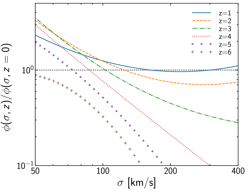
Figure 1: The redshift evolution of the velocity dispersion function adopted in this paper (equation 11). We show the velocity functions at several different redshifts relative to the local velocity function at $z=0$ as a function of the velocity dispersion $\sigma$.

While we mostly follow the methodology developed in Oguri & Marshall (2010), here we include several updates of calculations. First, in this paper we use an updated velocity dispersion function of all-type galaxies derived from the Sloan Digital Sky Survey Data Release 6 (Bernardi et al., 2010)

$$\phi_{\rm loc}(\sigma)=\phi_{*}\left(\frac{\sigma}{\sigma_{*}}\right)^{\alpha}\exp\left[-\left(\frac{\sigma}{\sigma_{*}}\right)^{\beta}\right]\frac{\beta}{\Gamma(\alpha/\beta)}\frac{1}{\sigma},$$ (10)

with $\phi_{*}=2.099\times 10^{-2}(h/0.7)^{3}{\rm Mpc^{-3}}$, $\sigma_{*}=113.78~{}{\rm km\,s^{-1}}$, $\alpha=0.94$, and $\beta=1.85$. We note that Oguri & Marshall (2010) adopted a velocity function of early type galaxies derived by Choi, Park, & Vogeley (2007). Different choices of a velocity function result in nearly a factor of two difference in total strong lensing probabilities, and therefore the same factor of difference in the magnification PDF at high magnifications. Since we are interested in strong lensing of very high-redshift sources, redshifts of lensing galaxies can also be relatively high. In Oguri & Marshall (2010), the velocity dispersion function is assumed to not evolve with redshift, which may be a reasonable assumption out to $z\sim 1.5$ (e.g. Bezanson et al., 2011). In this paper, however, we are interested in strong lensing of very high redshift sources for which redshifts of lensing galaxies can be much higher than $z\sim 1.5$. In order to take account of the redshift evolution of the velocity dispersion function, we adopt the result of Torrey et al. (2015) in which the redshift evolution of velocity dispersion functions is derived from the Illustris cosmological hydrodynamical simulation. Torrey et al. (2015) provided a velocity dispersion function $\phi_{\rm hyd}(\sigma,z)$ that fits results of the hydrodynamical simulation from $z=0$ to $6$. We combine this redshift dependence of the velocity dispersion function with the accurate local velocity dispersion function measurement by Bernardi et al. (2010) to derive the velocity dispersion function that is applicable for a wide range of redshift as

$$\phi(\sigma,z)=\phi_{\rm loc}(\sigma)\frac{\phi_{\rm hyd}(\sigma,z)}{\phi_{\rm hyd}(\sigma,0)}.$$ (11)

We show the redshift evolution of the velocity dispersion function derived from equation (11) in Figure 1. Since the strong lensing probability is proportional to $\sigma^{4}$, velocity dispersions of typical strong lensing galaxies correspond to the peak of $\sigma^{4}\phi(\sigma)$ and hence those of massive galaxies with high velocity dispersions. For these massive, high velocity dispersion galaxies, the redshift evolution is weak up to $z\sim 1$, but shows the strong decline of the number density at $z\ga 2$, which is in line with a native expectation from the redshift evolution of the mass function of dark matter haloes.

The density profile of each galaxy is same as that adopted in Oguri & Marshall (2010). We adopt the singular isothermal ellipsoid model for the galaxy, which is known to approximate the density profile of early type galaxies well, and add external shear. The probability distributions of the ellipticity and external shear are assumed to be same as those used in Oguri & Marshall (2010), i.e., the Gaussian distribution with mean of 0.3 and dispersion of 0.16 for the ellipticity and the lognormal distribution with mean 0.05 and dispersion 0.2 dex for the external shear. Their position angles are assumed to be completely random. In this paper, we ignore the dynamical normalization of the singular isothermal ellipsoid model for simplicity (see Oguri & Marshall, 2010).

We consider only galaxies as lensing objects, because total strong lensing cross sections for compact sources are dominated by those of single massive galaxies (e.g., Keeton, Kuhlen, & Haiman, 2005), which is also supported by the statistics of strong gravitational lenses discovered in submillimetre surveys (e.g., Amvrosiadis et al., 2018). This means that the inclusion of group- and cluster-scale haloes in the computation does not change our quantitative results significantly.

From the mock strong lens sample, we construct the source plane magnification PDF as a function of redshift, which we denote $dP_{\rm sl}/d\mu$. In the case of strong lensing, there is an ambiguity about how to deal with multiple images. In this paper, we regard multiple images as distinct images in computing the magnification PDF from the mock lens sample, because in observations of binary BH mergers it is not straightforward to identify multiple images. See Appendix A for more detailed discussions about the definition of magnification PDFs in the presence of multiple images.

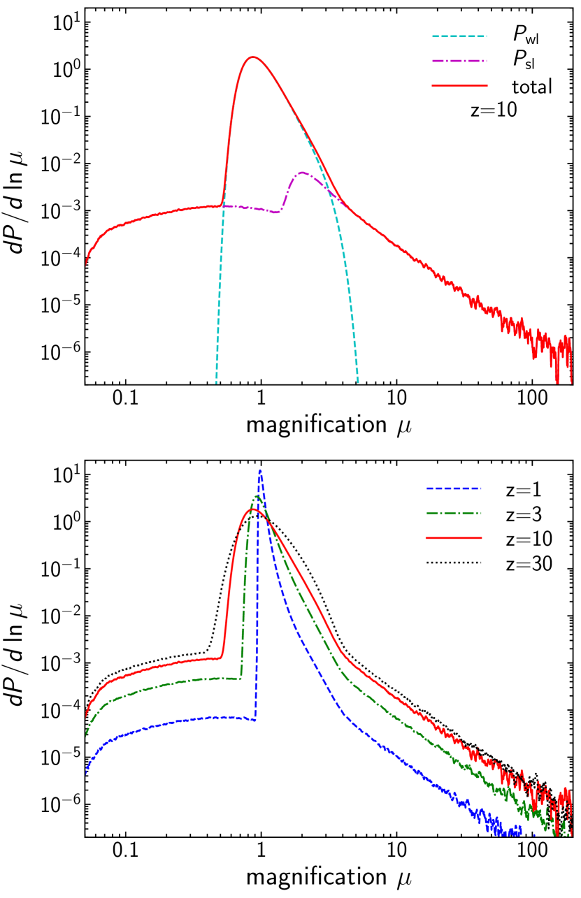
Figure 2: Top: The total magnification PDF for $z=10$ (solid) is shown together with contributions from magnification PDFs at low and high magnifications derived in Sections 2.1 and 2.2, respectively. These magnification PDFs derived using different methods are combined based on the methodology detailed in Appendix A, in which multiple images are treated separately. Bottom: The magnification PDFs for $z=1$ (dashed), $3$ (dash-dotted), $10$ (solid), and $30$ (dotted).

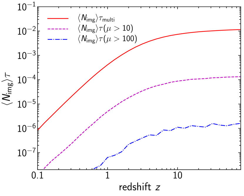
Figure 3: Optical depths $\langle N_{\rm img}\rangle\tau$ are plotted as a function of redshift. Here we define $\langle N_{\rm img}\rangle\tau$ regarding multiple images as distinct images (see text for more details). The solid line shows the optical depth for multiple images (equation 34), whereas the dashed and dash-dotted lines show the optical depths defined in equation (12) with $\mu_{\rm th}=10$ and $100$, respectively.

2.3 Combined magnification PDF

We follow the procedure detailed in Appendix A to combine magnification PDFs at low (Section 2.1) and high (Section 2.2) magnifications. As described in Appendix A, we include minor corrections in order to ensure the correct normalization and the mean magnification. The magnification PDFs are computed as a function of source redshift $z_{\rm s}$ with the source redshift bin size of 0.1 dex.

We show examples of magnification PDFs in Figure 2. As discussed in Appendix A, since we treat multiple images separately, the normalization of the magnification PDF exceeds unity, though only slightly. With increasing redshift, the magnification PDF becomes wide and has a higher tail at high magnifications. The feature seen at $\mu\sim 2$ for the magnification PDF from strong lensing, $P_{\rm sl}$ corresponds to the transition between magnified and demagnified images.

From the magnification PDF, we can compute the optical depth $\tau$ for strong lensing, which represents the probability of a source at redshift $z$ being strongly lensed. Again, since we treat multiple images separately, this optical depth differs from the conventional definition of the optical depth for which multiple images are grouped together. First we consider the optical depth for all multiple images, which was defined in equation (34). We also define the optical depth defined by the magnification threshold as

$$\langle N_{\rm img}\rangle\tau(>\mu_{\rm th})=\int^{\infty}_{\mu_{\rm th}}d\mu\frac{dP}{d\mu},$$ (12)

where we use the total magnification PDF for $dP/d\mu$, although at high magnifications it is dominated by that from strong lens mocks derived in Section 2.2. In Figure 3, we show optical depths with different definitions as a function of redshift. In all cases shown in the Figure, the optical depth rapidly increases as a function of redshift out to $z\sim 3$, but at high redshifts $z\ga 10$ the redshift dependence is rather weak.

3 Models of black hole binaries

Table 1: Parameters for BH merger rate density (equation 13) and the chirp mass distribution (equation 14) for three stellar origin models, Pop-I/II (Belczynski et al., 2017), Pop-III (B17) (Belczynski et al., 2017), and Pop-III (K16) (Kinugawa et al., 2016).

Parameters	Pop-I/II	Pop-III (B17)	Pop-III (K16)
$a_{1}$	$6.6\times 10^{3}$	$6\times 10^{4}$	$1\times 10^{4}$
$a_{2}$	1.6	1.0	0.7
$a_{3}$	2.1	1.4	1.1
$a_{4}$	30	$3\times 10^{6}$	500
$z_{\rm trunc}$	15	45	45
$b_{1}$	8	28	20
$b_{2}$	30	30	72

3.1 Stellar Origins

It has been known that BHs form naturally from the collapse of massive stars at the final stage of their evolution. This suggests that binary BHs may form from massive binary stars. Because the evolution of massive stars is sensitive to the metallicity due to its large impact on the mass loss rate, the merger rate density and masses of binary BHs are also expected to be sensitive to the metallicity. In addition, uncertainties associated with initial binary parameters make the prediction on the BH merger rate density quite uncertain (e.g., Belczynski, Kalogera, & Bulik, 2002; Belczynski et al., 2010, 2016, 2017; Dominik et al., 2012, 2013, 2015; Kinugawa et al., 2014, 2016; Hartwig et al., 2016).

In this paper, we consider a few model predictions from the population synthesis calculations as representative examples. Since the merger rate density and BH mass distribution depend sensitively on metallicity, those of metal free Population III (Pop-III) stars are expected to be markedly different from Population I and II (Pop-I/II) stars. For Pop-I/II stars, we adopt the model “M10” presented in Belczynski et al. (2017). For Pop-III stars, we consider a model presented in Kinugawa et al. (2016) (model “Standard”) and Belczynski et al. (2017) (“FS1”) to cover possible ranges of model predictions.

While in Belczynski et al. (2017) and Kinugawa et al. (2016) the redshift and mass distributions of BH mergers have been derived numerically with the binary population synthesis models, in this paper we adopt simple analytic forms for these distributions that roughly reproduce their numerical results. For the BH merger rate density, we assume the following functional form

$$\frac{R_{\rm GW}(z)}{\rm Gpc^{-3}yr^{-1}}=\frac{a_{1}e^{a_{2}z}}{e^{a_{3}z}+a_{4}},$$ (13)

for $z<z_{\rm trunc}$ and $R_{\rm GW}(z)=0$ at $z>z_{\rm trunc}$. On the other hand, we assume the following form for the chirp mass distribution of BH mergers

$$\frac{dp}{d\mathcal{M}}\propto\mathcal{M}^{-2.3}\left[1-e^{-(\mathcal{M}/b_{1})^{8}}\right]e^{-(\mathcal{M}/b_{2})^{8}}.$$ (14)

Note that the normalization is determined so as to satisfy $\int(dp/d\mathcal{M})d\mathcal{M}=1$. Parameters for these distributions are summarized in Table 1.

We show BH merger rate densities and chirp mass distributions for these three models in Figures 4 and 5, respectively.

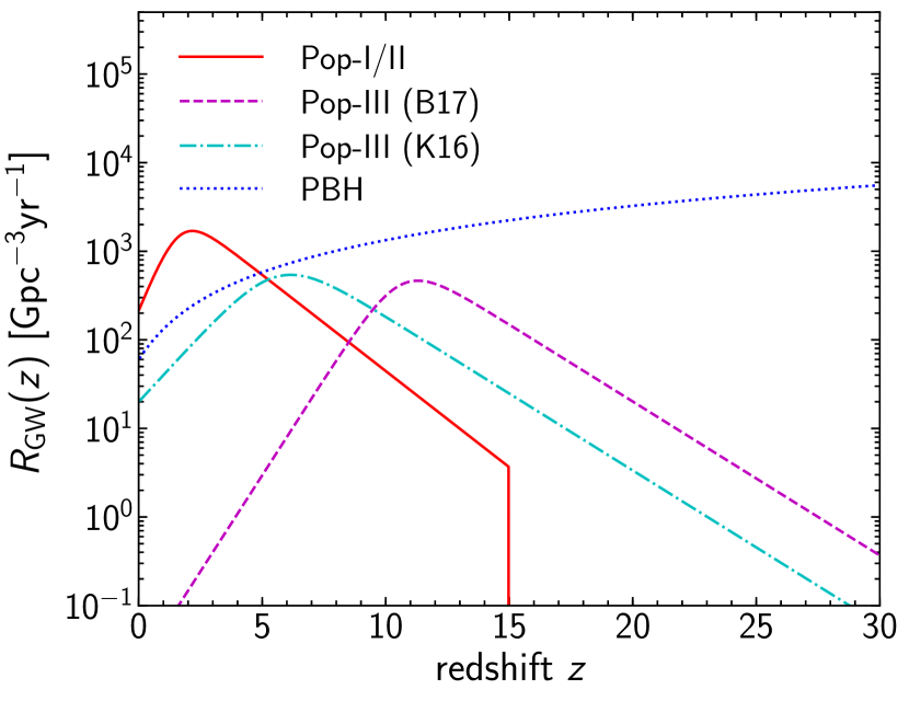
Figure 4: BH merger rate densities as a function of redshift for the three stellar origin models described in Section 3.1 and the PBH model described in Section 3.2.

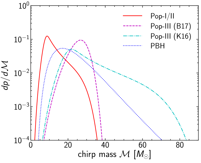
Figure 5: Distributions of the chirp mass for the three stellar origin models described in Section 3.1 and the PBH model described in Section 3.2.

3.2 Primordial black holes

Another scenario is that observed BH mergers may originate from PBHs (see Sasaki et al., 2018, for a review). In this paper, we consider a binary formation model considered in Sasaki et al. (2016), which originated from work by Nakamura et al. (1997). In this scenario, PBHs created in the early universe form a binary with high eccentricity due to the tidal effect of a neighboring PBH. Here we simply adopt the expression of the BH merger rate density as a function of redshift presented in Sasaki et al. (2016). We set the mass fraction of PBH, $f_{\rm PBH}=\Omega_{\rm PBH}/\Omega_{\rm DM}$, to $f_{\rm PBH}=5\times 10^{-3}$ so that it roughly matches the observed BH merger rate density (Abbott et al., 2016c).

Although a single PBH mass has been considered in Sasaki et al. (2016), in this paper we include the mass distribution of PBHs by assuming a log-normal form with the median chirp mass of $20~{}M_{\odot}$ and the scatter of $\ln\mathcal{M}$ of 0.4. The merger rate density and chirp mass distribution of the PBH model are compared with stellar origin models in Figures 4 and 5, respectively.

4 Calculation of the Distribution of binary black hole mergers

4.1 Signal-to-noise ratio

In this paper, we consider only the inspiral phase of gravitational waves to compute the expected signal-to-noise ratio for simplicity. This assumption has also been used in the literature to discuss detectabilities of binary BH mergers in future detectors (e.g., Taylor & Gair, 2012; Miyamoto et al., 2017; Li et al., 2018). In this case, the signal-to-noise ratio $\rho$ of binary BH mergers with masses $m_{1}$ and $m_{2}$ is computed as (Finn, 1996)

$$\rho=\sqrt{\frac{5}{96\pi^{4/3}}}\frac{R_{\odot}}{D_{\rm L}(z)}\left(\frac{\mathcal{M}_{z}}{M_{\odot}}\right)^{5/6}\Theta\sqrt{I}\equiv\rho_{0}\Theta,$$ (15)

$$R_{\odot}=cT_{\odot}=\frac{GM_{\odot}}{c^{2}},$$ (16)

$$\mathcal{M}_{z}=(1+z)\mathcal{M}=(1+z)\frac{(m_{1}m_{2})^{3/5}}{(m_{1}+m_{2})^{1/5}},$$ (17)

$$I=\int_{0}^{f_{\rm max}}df\,T_{\odot}^{-1/3}f^{-7/3}\{S_{n}(f)\}^{-1},$$ (18)

where $D_{\rm L}(z)$ is the luminosity distance, $\mathcal{M}_{z}$ is the redshifted chirp mass, and $S_{n}(f)$ is the noise power spectrum density of a detector which has the dimension of Hz^-1/2. The angular orientation function $\Theta$ encapsulates information on the detector with respect to the position of the binary BH merger on the sky as well as the inclination angle of the merger event. Assuming the random orientations, the PDF of $\Theta$ can be well approximated by (Finn, 1996)

$$P(\Theta)=\frac{5\Theta(4-\Theta)^{3}}{256},$$ (19)

for $0<\Theta<4$ and $P(\Theta)=0$ otherwise. We assume that $f_{\rm max}$ corresponds to the frequency at the innermost stable circular orbit (ISCO) that is given by

$$f_{\rm ISCO}=\frac{M_{\odot}}{6^{3/2}\pi T_{\odot}(1+z)M}\approx\frac{4397\,{\rm Hz}}{(1+z)(M/M_{\odot})},$$ (20)

where $M=m_{1}+m_{2}$ is the total mass of the binary BH system. For simplicity, throughout the paper we assume that masses of binary BHs are always equal e.g., $M=2^{6/5}\mathcal{M}$, to compute $f_{\rm ISCO}$.

4.2 Distribution of binary BH mergers

First we derive the event rate of binary BH mergers for a given gravitational wave observatory without the effect of gravitational lensing magnification. Assuming a threshold of the signal-to-noise ratio of $\rho_{\rm th}$, the event rate $R_{\rm obs}$ is computed as

$$R_{\rm obs}=\int dz\int d\mathcal{M}\frac{dV}{dz}\frac{R_{\rm GW}(z)}{1+z}\frac{dp}{d\mathcal{M}}S(\rho_{\rm th};\mathcal{M},z),$$ (21)

where $R_{\rm GW}(z)$ and $dp/d\mathcal{M}$ are the BH merger rate density and the chirp mass distribution, respectively, presented in Section 4, $dV/dz$ is the comoving volume element, and a factor $1/(1+z)$ takes account of the cosmological time dilation. The effect of the signal-to-noise ratio threshold $\rho_{\rm th}$ is included in $S(\rho_{\rm th};\mathcal{M},z)$ as

$$S(\rho_{\rm th};\mathcal{M},z)=T(4)-T(\rho_{\rm th}/\rho_{0}),$$ (22)

$$T(\Theta)=\frac{\Theta^{2}}{256}(160-80\Theta+15\Theta^{2}-\Theta^{3}),$$ (23)

for $\rho_{\rm th}/\rho_{0}<4$ and $S(\rho_{\rm th};\mathcal{M},z)=0$ otherwise.

Next we consider the effect of gravitational lensing magnification. Ignoring the effect of the phase shift (Dai & Venumadhav, 2017), we can include the effect of lensing magnification $\mu$ in the geometric optics limit simply by shifting the luminosity distance as

$$D_{\rm L}(z)\rightarrow\frac{D_{\rm L}(z)}{\sqrt{\mu}}.$$ (24)

Therefore, in presence of the lensing effect, the event rate is computed as

$$R_{\rm obs} = \int dz\int d\mu\frac{dP}{d\mu}\int d\mathcal{M}\frac{dV}{dz}\frac{R_{\rm GW}(z)}{1+z}\frac{dp}{d\mathcal{M}}$$ (25)

$$\times S_{\rm lens}(\rho_{\rm th};\mathcal{M},z,\mu),$$

$$S_{\rm lens}(\rho_{\rm th};\mathcal{M},z,\mu)=T(4)-T(\rho_{\rm th}/(\sqrt{\mu}\rho_{0})),$$ (26)

for $\rho_{\rm th}/(\sqrt{\mu}\rho_{0})<4$ and $S_{\rm lens}(\rho_{\rm th};\mathcal{M},z,\mu)=0$ otherwise, and $dP/d\mu$ is the magnification PDF as a function of redshift derived in Section 2.

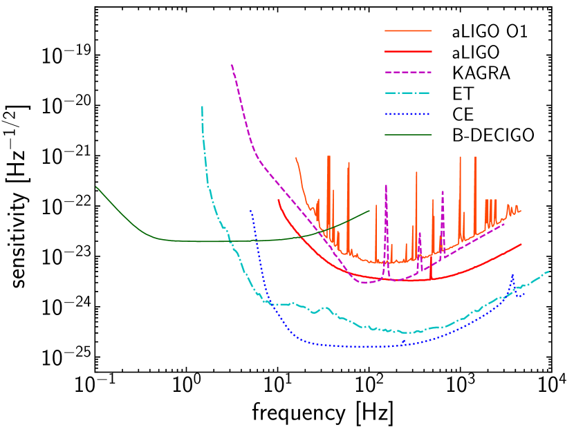
Figure 6: Noise power spectra $S_{n}(f)$ for various gravitational wave observatories that are considered in this paper. The sensitivity of advanced LIGO O1 is also shown for reference.

In this paper, we consider how gravitational lensing modifies the observable distribution of BH mergers. Specifically, we consider the differential distributions of the “observed redshift” $z_{\rm obs}$, which is the redshift inferred from the luminosity distance without the correction of lensing magnification $\mu$, as well as the “observed chirp mass” $\mathcal{M}_{\rm obs}$, which is the chirp mass inferred from the observed waveform, again without the correction of lensing magnification. They are simply defined as

$$D_{\rm L}(z_{\rm obs})=\frac{D_{\rm L}(z)}{\sqrt{\mu}},$$ (27)

$$\mathcal{M}_{\rm obs}=\frac{1+z}{1+z_{\rm obs}}\mathcal{M}.$$ (28)

By differentiating equation (25) we can obtain differential distribution of the event rate, $dR_{\rm obs}/dz_{\rm obs}$ and $dR_{\rm obs}/d\mathcal{M}_{\rm obs}$.

4.3 Gravitational wave observatories

In our calculation, information on gravitational wave observatories is included in the noise power spectrum $S_{n}(f)$. As specific examples, we consider $S_{n}(f)$ from ongoing observatories such as advanced LIGO (aLIGO) for the design specification and KAGRA (Nakamura et al., 2016), as well as the so-called third generation observatories such as Einstein Telescope (ET; Regimbau et al., 2012) and Cosmic Explorer (CE; Abbott et al., 2017). We also consider a planned space mission B-DECIGO (Nakamura et al., 2016) which is supposed to find binary BH mergers out to high redshifts. The noise power spectra assumed in this paper are shown in Figure 6.

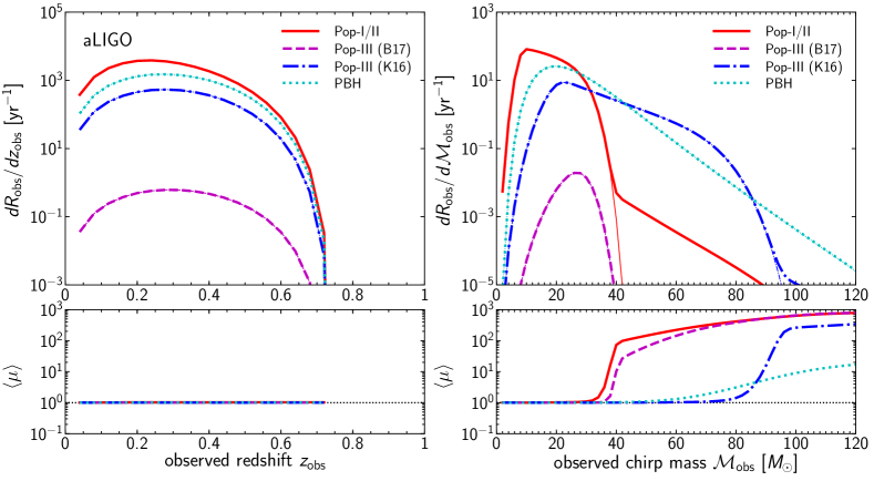
Figure 7: The differential distributions of the event rate for advanced LIGO. The left panel shows distributions of the observed redshift $z_{\rm obs}$ defined in equation (27), whereas the right panel shows distributions of the observed chirp mass define in equation (28). We plot distributions for the four binary BH merger models shown in Figures 4 and 5. For each model, thick lines show the distributions with the effect of gravitational lensing magnification (equation 25) and thin lines show the distributions without the lensing effect (equation 21). The mean magnifications are shown in the lower panels.

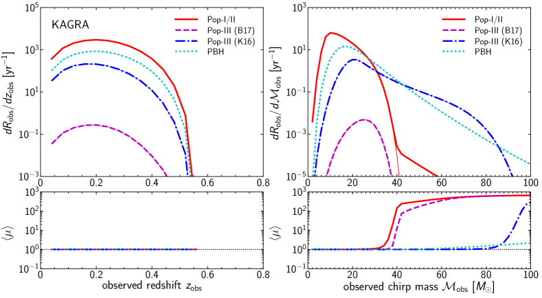
Figure 8: Same as Figure 7, but for KAGRA.

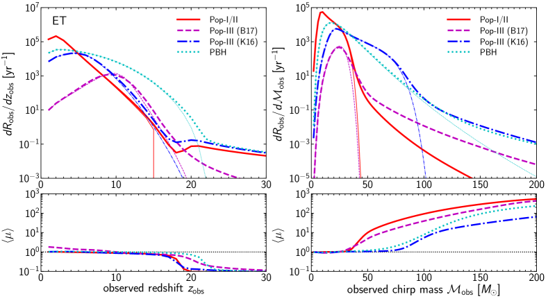
Figure 9: Same as Figure 7, but for Einstein Telescope.

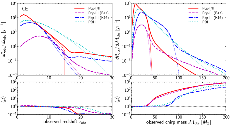
Figure 10: Same as Figure 7, but for Cosmic Explorer.

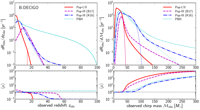
Figure 11: Same as Figure 7, but for B-DECIGO.

5 Results

5.1 Distributions in various observatories

We first derive differential distributions as a function of observed redshift $z_{\rm obs}$ (equation 27) as well as observed chirp mass $\mathcal{M}_{\rm obs}$ (equation 28) for various gravitational wave observatories summarized in Section 4.3. Throughout the paper we adopt the signal-to-noise threshold of $\rho_{\rm th}=8$ to compute expected distributions. Figures 7, 8, 9, 10, and 11 show event rate distributions for advanced LIGO, KAGRA, Einstein Telescope, Cosmic Explorer, and B-DECIGO, respectively. Here we ignore the measurement errors and show distributions that would be observed in absence of any measurement errors. Even without measurement errors, the event rate distributions are modified due to gravitational lensing magnification that we cannot be corrected for individual event basis.

We find that the differential distributions are modified due to gravitational lensing magnification, mainly at high $z_{\rm obs}$ and high $\mathcal{M}_{\rm obs}$. The high mass tail of the chirp mass distribution produced by lensing magnification has been discussed in the literature (e.g., Dai, Venumadhav, & Sigurdson, 2017; Broadhurst, Diego, & Smoot, 2018), which is due to highly magnified binary BH merger events. To explicitly check this point in our calculation, we compute the mean magnification as a function of the observed chirp mass from equation (25) as

$$\langle\mu\rangle(\mathcal{M}_{\rm obs}) = \left(\frac{dR_{\rm obs}}{d\mathcal{M}_{\rm obs}}\right)^{-1}\int dz\int d\mu\,\mu\frac{dP}{d\mu}\frac{d\mathcal{M}}{d\mathcal{M}_{\rm obs}}$$ (29)

$$\times\frac{dV}{dz}\frac{R_{\rm GW}(z)}{1+z}\frac{dp}{d\mathcal{M}}S_{\rm lens}(\rho_{\rm th};\mathcal{M},z,\mu).$$

The mean magnifications shown in the Figures clearly indicate that the tail at high $\mathcal{M}_{\rm obs}$ is driven by high magnification events.

Furthermore, we find that gravitational lensing magnification produces a high redshift tail in the $z_{\rm obs}$ distribution. The distribution of mean magnification computed in a manner similar to equation (29) indicates that this excess is driven by demagnified events. Our magnification PDF shown in Figure 2 suggests that such demagnified ($\mu\sim 0.1$) events are due to strong gravitational lensing. Strong lensing produces multiple images such that total magnifications of these multiple images are always larger than unity, but some of the multiple images can have $\mu<1$. Because of the difficulty in identifying multiple images in gravitational wave observations, these demagnified images are also assumed to be observed as distinct events, but due to lensing demagnifications they have observed redshifts much larger than their true redshifts, i.e., $z_{\rm obs}>z$.

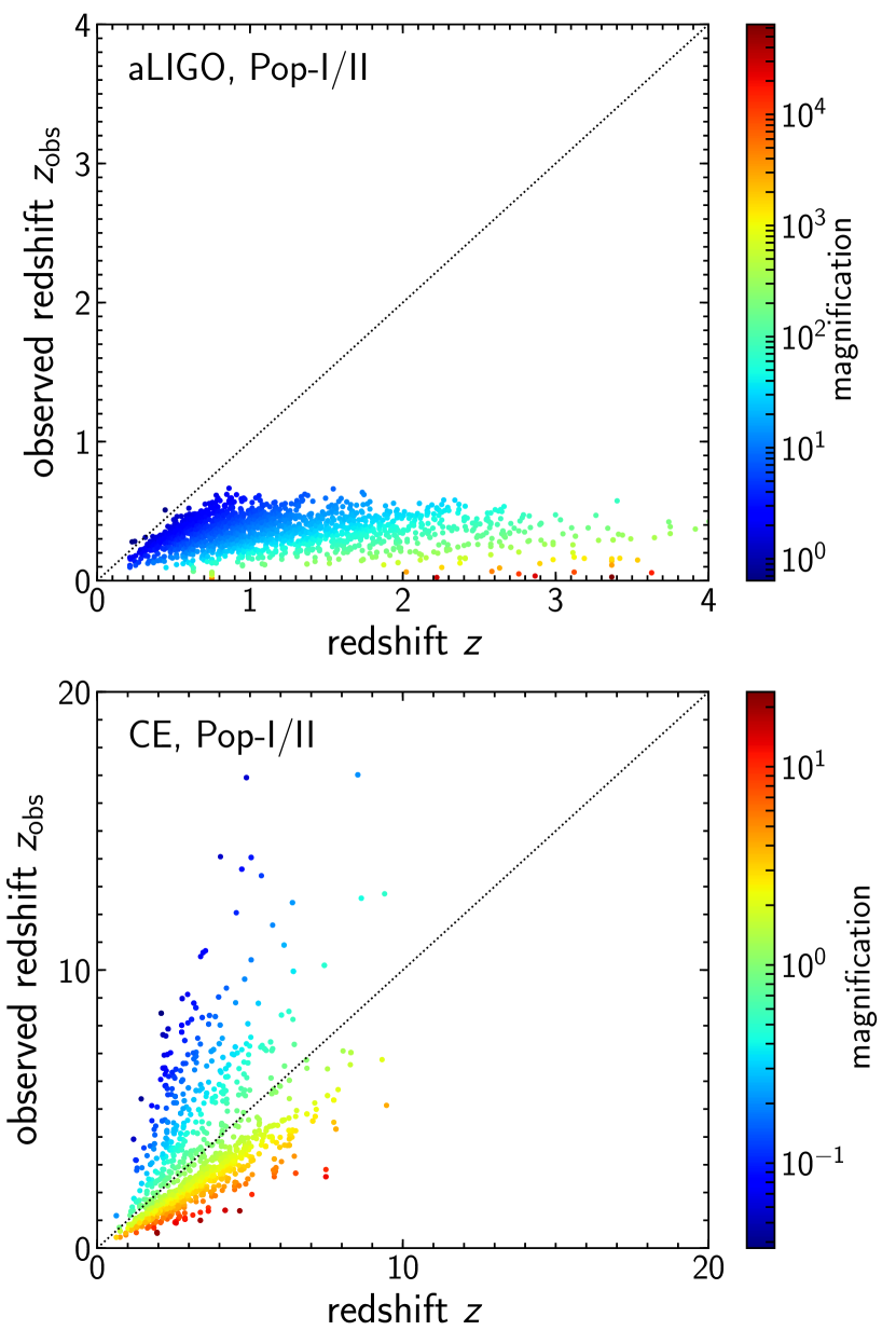
Figure 12: The distribution of mock multiple images for advanced LIGO (upper) and Cosmic Explorer (lower) in the $z$-$z_{\rm obs}$ plane, for the case of the Pop-I/II model. We plot mock data from 3000 years and 1 year observations for advanced LIGO and Cosmic Explorer, respectively.

5.2 Mock strong lens catalogues

As shown in the previous Section, high $\mathcal{M}_{\rm obs}$ and high $z_{\rm obs}$ events can be dominated by very high and low magnifications, respectively, both of which are produced by strong lensing (see also Figure 2). An advantage of our hybrid approach to compute the magnification PDF is that it also allows us to explore expected properties of multiple image pairs in detail, including expected time delays between these multiple images.

To explore the property of multiple images in detail, we construct mock multiple image catalogues following the methodology developed in Oguri & Marshall (2010). We first generate a large mock sample of gravitational wave events for a given model of the merger rate and chirp mass distributions. For each mock event, we check whether it is multiply imaged or not, using the lens model described in Section 2.2. When multiple images are generated, for each image we compute the signal-to-noise ratio using equation (15) taking account of gravitational lensing magnification via equation (24). For each image, we randomly assign the parameter $\Theta$ following the PDF of $\Theta$ presented in equation (19) to keep the consistency with the calculation presented in the previous Section. However we caution that this assumption may be inaccurate, particularly for image pairs with very short time delays, as the parameter $\Theta$ for these close pair events should be correlated rather than independent. We collect events with their signal-to-noise ratio larger than $\rho_{\rm th}=8$ to construct a mock catalogue for a given model and observatory.

This mock strong lens catalogue allows us to explore the relation between various parameters. As a specific example, we check the distribution of mock strong lens events in the $z$-$z_{\rm obs}$ plane. They are related with each other via equation (27), which indicates that the deviation from $z=z_{\rm obs}$ is simply caused by gravitational lensing magnification. Figure 12 shows the distributions in the $z$-$z_{\rm obs}$ plane for advanced LIGO and Cosmic Explorer as examples of second- and third-generation observatories, respectively. As shown in the Figure, there is a qualitative difference between the distributions for advanced LIGO and Cosmic Explorer. In the former case, detectable strong lens events are dominated by highly magnified events, and hence the observed redshift $z_{\rm obs}$ is always lower than the true redshift. On the other hand, in the case of Cosmic Explorer we can observe both magnified and demagnified events, so that there are events both at $z>z_{\rm obs}$ and $z<z_{\rm obs}$.

This qualitative difference can be explained by the selection effect. As shown in Figure 3, the lensing optical depth is very steep function of redshift out to $z\sim 1$. Because of this steep growth of the lensing optical depth, strong lens events observed in the second-generation observatories should be dominated by highly magnified high-redshift events (see also Broadhurst, Diego, & Smoot, 2018, for an extreme example). For the specific example shown in Figure 3, the median magnification for this strong lens sample is $\langle\mu\rangle\sim 14$. Such high median magnification due to the selection effect was also seen in observations of strongly lensed supernovae. Strongly lensed Type Ia supernovae recently discovered in relatively shallow surveys, PS1-10afx (Quimby et al., 2014) and iPTF16geu (Goobar et al., 2017), have high total magnifications of $\mu\sim 30-50$ for the same reason as discussed above (see also Quimby et al., 2014). In most cases, the low-magnification counterimages of these high magnification images are not observable due to their low signal-to-noise ratios.

In contrast, in the case of Cosmic Explorer we can observe both magnified and demagnified events. This is because we can detect many binary BH mergers at $z\sim 2-5$ with Cosmic Explorer without lensing magnifications (see Figure 10), and thanks to the high sensitive of the observatory, demagnified image of strong lens events at these redshifts can also be detected easily. These demagnified multiple images are the origin of apparently very high observed redshift ($z_{\rm obs}\ga 15$) events shown in Figure 10.

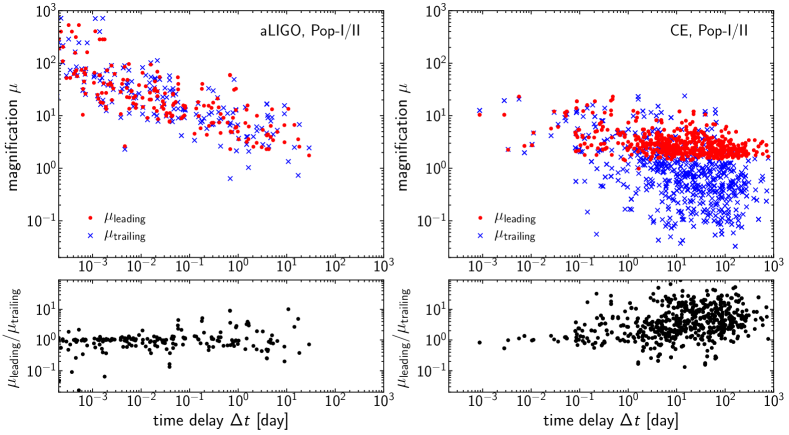
Figure 13: Distributions of time delays and magnifications for pairs of multiple images from the mock strong lens catalogues. As in Figure 12, we plot mock data of the Pop-I/II model from 3000 years and 1 year observations for advanced LIGO (left) and Cosmic Explorer (right), respectively. The upper panels show time delays and magnifications of leading (filled circles) and trailing (crosses) images for any image pairs in the mock catalogues. The bottom panels show time delays and ratios of magnifications of leading and trailing images.

Table 2: Summary of predicted event rates for various observatories and models of binary BH mergers. $R_{\rm obs}$ denotes the total number of observed events per year, $R_{\rm sl}$ is the total number of strongly lensed events per year, $\langle\mu_{\rm sl}\rangle$ is the median magnification of strongly lensed events, $R_{\rm pair}$ is the total number of observed multiple image pairs per year, $\Delta t$ is the median time delay of the observed multiple image pairs, and $\langle\mu_{\rm leading}/\mu_{\rm trailing}\rangle$ is the median value of the ratio of magnifications of leading and trailing images of the observed multiple image pairs. Values of $\langle\mu_{\rm sl}\rangle$, $R_{\rm pair}$, $\Delta t$, and $\langle\mu_{\rm leading}/\mu_{\rm trailing}\rangle$ are derived from the strong lens mock catalogues (see Section 5.2). Values in parentheses for $\langle\mu_{\rm sl}\rangle$, $\Delta t$, and $\langle\mu_{\rm leading}/\mu_{\rm trailing}\rangle$ denote 68% ranges, again derived from the strong lens mock catalogues. For aLIGO/Pop-III (B17) and KAGRA/Pop-III (B17), we fail to construct mock lens catalogues because they predict too low strong lens event rates.

observatory/model	$R_{\rm obs}$ [yr-1]	$R_{\rm sl}$ [yr-1]	$\langle\mu_{\rm sl}\rangle$	$R_{\rm pair}$ [yr-1]	$\Delta t$ [day]	$\langle\mu_{\rm leading}/\mu_{\rm trailing}\rangle$
aLIGO/Pop-I/II	1.14e+03	5.84e$-$01	14.35 (3.39–72.71)	7.77e$-$02	0.006 (0.000–0.739)	1.00 (0.61–1.23)
aLIGO/Pop-III (B17)	2.00e$-$01	6.21e$-$05	—	—	—	—
aLIGO/Pop-III (K16)	1.68e+02	3.89e$-$02	6.32 (2.50–27.97)	3.33e$-$03	0.433 (0.013–2.906)	1.22 (0.82–1.37)
aLIGO/PBH	4.75e+02	1.35e$-$01	6.89 (2.40–32.84)	1.43e$-$02	0.124 (0.002–2.853)	0.92 (0.48–1.54)
KAGRA/Pop-I/II	6.84e+02	1.69e$-$01	17.49 (3.30–105.11)	2.37e$-$02	0.002 (0.000–0.090)	1.00 (0.52–1.19)
KAGRA/Pop-III (B17)	5.58e$-$02	3.81e$-$06	—	—	—	—
KAGRA/Pop-III (K16)	4.59e+01	3.10e$-$03	7.65 (2.51–83.11)	6.67e$-$04	0.005 (0.002–0.008)	1.01 (1.00–1.01)
KAGRA/PBH	1.93e+02	2.00e$-$02	7.27 (2.65–45.64)	3.33e$-$03	0.546 (0.139–1.081)	1.05 (0.81–1.79)
ET/Pop-I/II	5.54e+05	1.12e+03	2.10 (0.88–3.55)	4.56e+02	13.741 (1.184–83.138)	2.36 (0.91–6.75)
ET/Pop-III (B17)	5.96e+03	7.38e+01	2.41 (1.70–4.32)	1.50e+01	16.518 (0.736–79.897)	1.95 (0.70–5.10)
ET/Pop-III (K16)	1.13e+05	4.86e+02	2.10 (0.83–3.40)	1.74e+02	15.094 (1.328–96.548)	2.61 (0.93–6.91)
ET/PBH	2.27e+05	1.18e+03	2.25 (1.36–3.93)	3.55e+02	12.942 (1.042–80.279)	2.06 (0.80–5.60)
CE/Pop-I/II	7.31e+05	1.60e+03	1.88 (0.38–3.09)	8.36e+02	20.600 (2.318–113.044)	3.64 (1.24–11.20)
CE/Pop-III (B17)	1.54e+03	1.51e+01	2.44 (1.88–3.98)	2.60e+00	8.266 (0.501–208.184)	3.02 (1.02–6.55)
CE/Pop-III (K16)	9.96e+04	3.96e+02	2.07 (0.60–3.64)	1.82e+02	21.283 (1.444–107.229)	2.90 (0.92–8.78)
CE/PBH	2.47e+05	1.07e+03	2.05 (0.71–3.49)	4.63e+02	18.806 (1.290–108.130)	2.68 (1.01–8.18)
B-DECIGO/Pop-I/II	2.02e+05	4.71e+02	2.36 (1.63–4.19)	9.98e+01	8.252 (0.595–56.830)	1.70 (0.78–4.65)
B-DECIGO/Pop-III (B17)	5.96e+03	9.20e+01	2.50 (1.76–4.84)	1.92e+01	3.430 (0.188–21.441)	1.23 (0.50–2.82)
B-DECIGO/Pop-III (K16)	7.66e+04	3.86e+02	2.27 (1.47–3.94)	1.22e+02	14.577 (1.060–86.073)	1.88 (0.78–4.78)
B-DECIGO/PBH	1.31e+05	1.41e+03	2.63 (1.81–5.43)	2.70e+02	4.965 (0.264–50.640)	1.29 (0.57–3.29)

5.3 Time delays between observed multiple image pairs

One application of the mock strong lens catalogues constructed in Section 5.2 is that they allow us to estimate distributions of time delays between multiple image pairs. From the strong lens mock, we select all pairs of multiple images both of which are detected, i.e., $\rho>\rho_{\rm th}$. Our mock catalogues contain strong lens events with more than two (typically four) images. When more than two images are detected, we consider all the possible pairs of multiple images and derive time delays between all these pairs.

Figure 13 shows distributions of time delays and magnifications for all pairs of multiple images in the strong lens mock catalogues, again for advanced LIGO and Cosmic Explorer as examples of second- and third-generation observatories, respectively. In addition to the difference in typical magnifications, we find that typical time delays are also quite different between advanced LIGO and Cosmic Explorer.

In the case of advanced LIGO, we preferentially detect binary BH mergers that are highly magnified by gravitational lensing due to the selection effect. In most cases, such high magnifications are realized near the fold or cusp catastrophe, where pairs of multiple images with similar magnifications are produced. Because they share similar light paths, time delays between these high magnification image pairs are very short. We find that time delays for multiple image pairs from advanced LIGO are indeed short, typically less than a day. Given the relatively low total event rate of advanced LIGO, it should be relatively easy to identify strong lensing events from the occurrence of multiple events in a short time scale. Realistic estimates of the identifications of such multiple events require to take account of the effect of the Earth rotation as well as data glitches (see also Broadhurst, Diego, & Smoot, 2018). We leave the exploration of this for future work.

When a source is located very close to the caustic, the wave effect becomes important. This happens when the time delay between multiple images near the critical curve is comparable to the wave period (e.g., Nakamura & Deguchi, 1999). Figure 13 suggests that, even for images with very high magnifications, $\mu\sim 10^{3}$, time delays between multiple image pairs are typically larger than a second and therefore are much larger than the inverse of frequency of ground-based gravitational wave observations. Thus the wave effect can be neglected even for these highly magnified image pairs.

On the other hand, in the case of Cosmic Explorer we can detect many multiple image pairs from more typical asymmetric image configurations with large magnification differences. Such asymmetric image configurations produce image pairs with large time delays. We find that typical time delays are $10-100$ days, which are much longer than time delays in the case of advanced LIGO. Together with the high total event rates, this relatively long time delays make it challenging to distinguish such multiple images from two distinct single image events. Furthermore, long time delays suggest that some of multiple images cannot be detected in a given observing run, because one of the multiple images can arrive before or after the observing run. This “time delay bias” has been considered in Oguri, Suto, & Turner (2003) in the context of gravitationally lensed supernovae, and was also discussed in Li et al. (2018).

Figure 13 indicates that there is a clear difference in the distributions of magnifications between leading and trailing images of multiple image pairs. In particular, this Figure suggests that highly demagnified images, which produce a high redshift tail in the $z_{\rm obs}$ distribution, almost always correspond to trailing images. This indicates that, when a very high $z_{\rm obs}$ event due to lensing demagnification is detected, such even should be accompanied by a much lower $z_{\rm obs}$ event that is observed $\sim 10-100$ days before the high $z_{\rm obs}$ event. Waveforms of these two multiple image events with high and low $z_{\rm obs}$ should be similar except for their overall amplitudes. In practice, demagnified events receive additional frequency dependent phase shift, which may help identify these strongly lensed multiple image pairs (Dai & Venumadhav, 2017).

Table 2 summarizes predicted event rates for various observatories and models of binary BH mergers. Again, this Table highlights the large difference between ongoing (advanced LIGO and KAGRA) and future (Einstein Telescope, Cosmic Explorer, and B-DECIGO) observatories on typical values of magnifications of time delays. The fractions of strongly lensed events are found to $\sim 10^{-4}$ for advanced LIGO and KAGRA and $\sim 10^{-2}-10^{-3}$ for Einstein Telescope, Cosmic Explorer, and B-DECIGO.

6 Summary

In this paper, we have explored the effect of gravitational lensing magnification on the distribution of binary BH mergers observed by gravitational wave observatories. For this purpose, we have developed a hybrid model of the PDF of gravitational lensing magnification, in which the effects of weak and strong gravitational lensing are combined. In particular, we derive the magnification PDF by treating multiple images separately (see Appendix A), which should be appropriate here given the poor angular resolution of gravitational wave observatories as well as faint electromagnetic counterparts if at all exist.

We have found that pronounced effects of gravitational lensing magnifications appear at high observed chirp mass $\mathcal{M}_{\rm obs}$ (equation 28) and at high observed redshift $z_{\rm obs}$ (equation 27). The heavy tail of the distribution at high $\mathcal{M}_{\rm obs}$ is due to highly magnified strong lens events, which has been recognized in previous work (Dai, Venumadhav, & Sigurdson, 2017; Smith et al., 2018; Broadhurst, Diego, & Smoot, 2018). We have found that highly demagnified images of strong lensing events also produce a heavy tail of the distribution at high $z_{\rm obs}$, which can be easily detected in future gravitational wave observatories. It has been argued that the presence or absence of very high redshift BH merger events provide an importance clue for discriminating various binary BH formation models (Nakamura et al., 2016; Koushiappas & Loeb, 2017), but our work demonstrates that the effect of gravitational lensing has to be taken into account carefully in order to properly interpret apparently very high redshift events.

Our hybrid approach enables us to explore the expected properties of strong lensing events detectable in individual gravitational wave observatories. For instance, in ongoing gravitational wave observatories such as advanced LIGO and KAGRA, we preferentially observe highly magnified strong lensing events due to the selection effect. As a result, we expect to observe pairs of strongly lensed events with similar magnifications and short time delays of $\la 1$ day, suggesting that we may be able to identify strongly lensed events from such image pairs with similar properties. On the other hand, in the next generation gravitation wave observatories such as Einstein Telescope and Cosmic Explorer, strong lensing events are dominated by those with “asymmetric” image configurations with large magnification ratios and large time delays between multiple images. Our mock catalogues of strong lens events indicate that highly demagnified images, which are important source of apparently high observed redshift events, should be accompanied by a magnified event that is observed typically $10-100$ days before the demagnified event. However, the expected long time delays may make it challenging to identify such pairs of strong lensing events with magnifications and demagnifications.

In this paper, we have adopted several simplified assumptions. While we have assigned the angular orientation function $\Theta$ completely randomly for different events, values of $\Theta$ should be correlated for image pairs with short time delays. We have also ignored measurement errors of observed redshifts and chirp masses when discussing their distributions. In order to discuss the possibility of identifying multiple image pairs, we need to take account of the localization accuracy on the sky as well as the chance probability of having distinct gravitational wave events with similar waveforms. Given the limited amount of information available from binary BH merger events, it is of great importance to explore the possibility of identifying multiple images in a realistic situation, in order to understand the origin of possible extreme events with very high $\mathcal{M}_{\rm obs}$ or $z_{\rm obs}$ detected in the future.

Appendix A Magnification PDFs in the presence of multiple images

In this paper, we are interested in the magnification PDF defined in the source plane, as gravitational wave sources are randomly distributed in the source plane rather than in the image plane. In the strong lens regime, the definition of the magnification is rather ambiguous because a single source produces multiple images. We argue that the relevant definition of the magnification factor depends on the observation and the identification scheme of multiple images. For instance, in survey observations with poor angular resolutions, such as an imaging survey in the sub-millimetre band (e.g., Negrello et al., 2010), multiple images are not resolved. In this case, it is appropriate to adopt the total magnification i.e., the sum of magnification factors of multiple images, as the definition of the magnification.

The situation is more complicated when multiple images are resolved. In the case of gravitational wave observations, while multiple images are not resolved spatially given their poor angular resolutions, they are almost always resolved temporally. However, as discussed in this paper, the identification of multiple images is not straightforward in gravitational wave observations again given their poor spatial resolutions. Thus in this paper we treat multiple images separately. In this case, the number of sources is not conserved by strong gravitational lensing i.e., the number of sources in the image plane differs from the number of sources in the source plane.

In practice, from the strong lens mock sample at a give source redshift constructed in Section 2.2, we derive two types of magnification PDFs. First, we derive the magnification PDF in which multiple images are grouped together. For $j$-th strong lens system, we compute the total magnification as

$$\mu_{j,{\rm tot}}=\sum_{k}\mu_{j,k},$$ (30)

where the summation $k$ runs over multiple images of the $j$-th mock strong lens system, and $\mu_{j,k}$ denotes the magnification of the individual image for the $j$-th mock strong lens system. We then compute the magnification PDF in the $i$-th magnification bin with $\mu_{i,{\rm min}}<\mu_{i}<\mu_{i,{\rm max}}$ as

$$\frac{dP_{\rm sl,lens}}{d\mu_{i}}=\frac{1}{N_{\rm s}}\sum_{j}\Theta(\mu_{j,{\rm tot}}-\mu_{i,{\rm min}})\Theta(\mu_{i,{\rm max}}-\mu_{j,{\rm tot}}),$$ (31)

where $\Theta$ is the Heaviside step function, $N_{s}$ is the total number of sources at this source redshift that are randomly distributed to generate the mock lens sample, and the summation runs over the mock lens sample. This magnification PDF is normalized such that the integral over the magnification gives the lensing optical depth $\tau_{\rm multi}$ i.e., the total probability of strong gravitational lensing with multiple images

$$\int d\mu\frac{dP_{\rm sl,lens}}{d\mu_{i}}=\tau_{\rm multi}.$$ (32)

Next, we define another magnification PDF for which multiple images of individual mock lens system are treated separately. Using the notations defined above, we can derive this magnification PDF as

$$\frac{dP_{\rm sl,img}}{d\mu_{i}}=\frac{1}{N_{\rm s}}\sum_{j}\sum_{k}\Theta(\mu_{j,k}-\mu_{i,{\rm min}})\Theta(\mu_{i,{\rm max}}-\mu_{j,k}).$$ (33)

This magnification PDF has a different normalization from $dP_{\rm sl,lens}/d\mu$. Specifically, $dP_{\rm sl,img}/d\mu$ is normalized such that

$$\int d\mu\frac{dP_{\rm sl,img}}{d\mu_{i}}=\langle N_{\rm img}\rangle\tau_{\rm multi},$$ (34)

where $\langle N_{\rm img}\rangle$ is the average number of multiple images for the mock strong lens systems. Since most strong lens systems have two or four multiple images, we expect $2<\langle N_{\rm img}\rangle<4$.

As shown in Section 2.3, we combine the magnification PDF from the strong lens mock sample with that at low magnification derived in Section 2.1 to obtain the total magnification PDF. However, if we simply sum up these magnification PDFs, the resulting magnification PDF does not satisfy the correct normalization condition. Therefore we tweak the normalization of the magnification PDF at low magnification to ensure the normalization

$$\frac{dP}{d\mu}=\frac{1-\tau_{\rm multi}}{\int d\mu\,dP_{\rm wl}/d\mu}\frac{dP_{\rm wl}}{d\mu}+\frac{dP_{\rm sl}}{d\mu}.$$ (35)

We note that the prefactor $(1-\tau_{\rm multi})/\int d\mu\,dP_{\rm wl}/d\mu$ is in fact quite close to unity with a typical deviation of $\sim 3$% or so, indicating that this correction is a minor correction. When we adopt $dP_{\rm sl}/d\mu=dP_{\rm sl,lens}/d\mu$, we can easily show that

$$\int d\mu\frac{dP}{d\mu}=1,$$ (36)

which is expected from the conservation of the number of sources by gravitational lensing. In contrast, when we adopt $dP_{\rm sl}/d\mu=dP_{\rm sl,img}/d\mu$, the number of sources no longer conserves as strong lensing, once multiple images are treated separately, increases the number of observed events. In this case, the normalization exceeds unity

$$\int d\mu\frac{dP}{d\mu}=1+\tau_{\rm multi}(\langle N_{\rm img}\rangle-1)>1,$$ (37)

although we note that $\tau_{\rm multi}\ll 1$ and hence the excess is small. As mentioned above, in this paper we adopt $dP_{\rm sl}/d\mu=dP_{\rm sl,img}/d\mu$ and treat multiple images separately.

The magnification PDF constructed above does not guarantees $\langle\mu\rangle=1$ which is expected for the source plane magnification PDF (e.g., Takahashi et al., 2011), even when we adopt the total magnification, $dP_{\rm sl}/d\mu=dP_{\rm sl,lens}/d\mu$. To correct for this, for each source redshift bin we compute the magnification shift parameter

$$\mu_{\rm shift}=1-\int d\mu\frac{dP}{d\mu}\mu,$$ (38)

where $dP/d\mu$ is computed using $dP_{\rm sl}/d\mu=dP_{\rm sl,lens}/d\mu$, and uniformly shift the magnification in the magnification PDF as

$$\mu\rightarrow\mu+\mu_{\rm shift},$$ (39)

which ensures $\langle\mu\rangle=1$. We apply this shift of the magnification even when we adopt $dP_{\rm sl}/d\mu=dP_{\rm sl,img}/d\mu$ that is used in our main analysis. Again, this shift is quite minor with $|\mu_{\rm shift}|\la 0.02$ for $z_{\rm s}\la 10$ and $|\mu_{\rm shift}|\la 0.1$ for $z_{\rm s}\la 100$.

References

- Abbott et al. (2016a) Abbott B. P., et al., 2016a, PhRvL, 116, 061102
- Abbott et al. (2016b) Abbott B. P., et al., 2016b, ApJ, 826, L13
- Abbott et al. (2016c) Abbott B. P., et al., 2016c, PhRvX, 6, 041015
- Abbott et al. (2017) Abbott B. P., et al., 2017, CQGra, 34, 044001
- Amvrosiadis et al. (2018) Amvrosiadis A., et al., 2018, MNRAS, 475, 4939
- Belczynski, Kalogera, & Bulik (2002) Belczynski K., Kalogera V., Bulik T., 2002, ApJ, 572, 407
- Belczynski et al. (2010) Belczynski K., Dominik M., Bulik T., O’Shaughnessy R., Fryer C., Holz D. E., 2010, ApJ, 715, L138
- Belczynski et al. (2016) Belczynski K., Holz D. E., Bulik T., O’Shaughnessy R., 2016, Natur, 534, 512
- Belczynski et al. (2017) Belczynski K., Ryu T., Perna R., Berti E., Tanaka T. L., Bulik T., 2017, MNRAS, 471, 4702
- Bernardi et al. (2010) Bernardi M., Shankar F., Hyde J. B., Mei S., Marulli F., Sheth R. K., 2010, MNRAS, 404, 2087
- Bertacca et al. (2018) Bertacca D., Raccanelli A., Bartolo N., Matarrese S., 2018, PDU, 20, 32
- Bezanson et al. (2011) Bezanson R., et al., 2011, ApJ, 737, L31
- Biesiada et al. (2014) Biesiada M., Ding X., Piórkowska A., Zhu Z.-H., 2014, JCAP, 10, 080
- Bird et al. (2016) Bird S., Cholis I., Muñoz J. B., Ali-Haïmoud Y., Kamionkowski M., Kovetz E. D., Raccanelli A., Riess A. G., 2016, PhRvL, 116, 201301
- Blandford & Narayan (1986) Blandford R., Narayan R., 1986, ApJ, 310, 568
- Broadhurst, Diego, & Smoot (2018) Broadhurst T., Diego J. M., Smoot G., III, 2018, arXiv, arXiv:1802.05273
- Camera & Nishizawa (2013) Camera S., Nishizawa A., 2013, PhRvL, 110, 151103
- Castro et al. (2018) Castro T., Quartin M., Giocoli C., Borgani S., Dolag K., 2018, MNRAS, 478, 1305
- Choi, Park, & Vogeley (2007) Choi Y.-Y., Park C., Vogeley M. S., 2007, ApJ, 658, 884
- Clesse & García-Bellido (2017) Clesse S., García-Bellido J., 2017, PDU, 15, 142
- Dai & Venumadhav (2017) Dai L., Venumadhav T., 2017, arXiv, arXiv:1702.04724
- Dai, Venumadhav, & Sigurdson (2017) Dai L., Venumadhav T., Sigurdson K., 2017, PhRvD, 95, 044011
- Das & Ostriker (2006) Das S., Ostriker J. P., 2006, ApJ, 645, 1
- Diego (2018) Diego J. M., 2018, arXiv, arXiv:1806.04668
- Ding, Biesiada, & Zhu (2015) Ding X., Biesiada M., Zhu Z.-H., 2015, JCAP, 12, 006
- Dominik et al. (2012) Dominik M., Belczynski K., Fryer C., Holz D. E., Berti E., Bulik T., Mandel I., O’Shaughnessy R., 2012, ApJ, 759, 52
- Dominik et al. (2013) Dominik M., Belczynski K., Fryer C., Holz D. E., Berti E., Bulik T., Mandel I., O’Shaughnessy R., 2013, ApJ, 779, 72
- Dominik et al. (2015) Dominik M., et al., 2015, ApJ, 806, 263
- Farr et al. (2017) Farr W. M., Stevenson S., Miller M. C., Mandel I., Farr B., Vecchio A., 2017, Natur, 548, 426
- Fialkov & Loeb (2015) Fialkov A., Loeb A., 2015, ApJ, 806, 256
- Finn (1996) Finn L. S., 1996, PhRvD, 53, 2878
- Goobar et al. (2017) Goobar A., et al., 2017, Sci, 356, 291
- Hamana, Martel, & Futamase (2000) Hamana T., Martel H., Futamase T., 2000, ApJ, 529, 56
- Hartwig et al. (2016) Hartwig T., Volonteri M., Bromm V., Klessen R. S., Barausse E., Magg M., Stacy A., 2016, MNRAS, 460, L74
- Hilbert et al. (2007) Hilbert S., White S. D. M., Hartlap J., Schneider P., 2007, MNRAS, 382, 121
- Hilbert et al. (2008) Hilbert S., White S. D. M., Hartlap J., Schneider P., 2008, MNRAS, 386, 1845
- Holz & Wald (1998) Holz D. E., Wald R. M., 1998, PhRvD, 58, 063501
- Holz & Hughes (2005) Holz D. E., Hughes S. A., 2005, ApJ, 629, 15
- Kainulainen & Marra (2011) Kainulainen K., Marra V., 2011, PhRvD, 83, 023009
- Kaiser & Peacock (2016) Kaiser N., Peacock J. A., 2016, MNRAS, 455, 4518
- Keeton, Kuhlen, & Haiman (2005) Keeton C. R., Kuhlen M., Haiman Z., 2005, ApJ, 621, 559
- Kinugawa et al. (2014) Kinugawa T., Inayoshi K., Hotokezaka K., Nakauchi D., Nakamura T., 2014, MNRAS, 442, 2963
- Kinugawa et al. (2016) Kinugawa T., Miyamoto A., Kanda N., Nakamura T., 2016, MNRAS, 456, 1093
- Kochanek & White (2001) Kochanek C. S., White M., 2001, ApJ, 559, 531
- Kocsis et al. (2018) Kocsis B., Suyama T., Tanaka T., Yokoyama S., 2018, ApJ, 854, 41
- Koushiappas & Loeb (2017) Koushiappas S. M., Loeb A., 2017, PhRvL, 119, 221104
- Lapi et al. (2012) Lapi A., Negrello M., González-Nuevo J., Cai Z.-Y., De Zotti G., Danese L., 2012, ApJ, 755, 46
- Li et al. (2018) Li S.-S., Mao S., Zhao Y., Lu Y., 2018, MNRAS, 476, 2220
- Liao et al. (2017) Liao K., Fan X.-L., Ding X., Biesiada M., Zhu Z.-H., 2017, NatCo, 8, 1148
- Lima, Jain, & Devlin (2010) Lima M., Jain B., Devlin M., 2010, MNRAS, 406, 2352
- Marković (1993) Marković D., 1993, PhRvD, 48, 4738
- Miyamoto et al. (2017) Miyamoto A., Kinugawa T., Nakamura T., Kanda N., 2017, PhRvD, 96, 064025
- Nakamura & Deguchi (1999) Nakamura T. T., Deguchi S., 1999, PThPS, 133, 137
- Nakamura et al. (1997) Nakamura T., Sasaki M., Tanaka T., Thorne K. S., 1997, ApJ, 487, L139
- Nakamura et al. (2016) Nakamura T., et al., 2016, PTEP, 2016, 093E01
- Namikawa, Nishizawa, & Taruya (2016) Namikawa T., Nishizawa A., Taruya A., 2016, PhRvL, 116, 121302
- Negrello et al. (2010) Negrello M., et al., 2010, Sci, 330, 800
- Ng et al. (2018) Ng K. K. Y., Wong K. W. K., Broadhurst T., Li T. G. F., 2018, PhRvD, 97, 023012
- Oguri (2010) Oguri M., 2010, PASJ, 62, 1017
- Oguri (2016) Oguri M., 2016, PhRvD, 93, 083511
- Oguri & Marshall (2010) Oguri M., Marshall P. J., 2010, MNRAS, 405, 2579
- Oguri, Suto, & Turner (2003) Oguri M., Suto Y., Turner E. L., 2003, ApJ, 583, 584
- O’Leary, Meiron, & Kocsis (2016) O’Leary R. M., Meiron Y., Kocsis B., 2016, ApJ, 824, L12
- Osato (2018) Osato K., 2018, arXiv, arXiv:1807.00016
- Perrotta et al. (2002) Perrotta F., Baccigalupi C., Bartelmann M., De Zotti G., Granato G. L., 2002, MNRAS, 329, 445
- Planck Collaboration et al. (2016) Planck Collaboration, et al., 2016, A&A, 594, A13
- Quimby et al. (2014) Quimby R. M., et al., 2014, Sci, 344, 396
- Regimbau et al. (2012) Regimbau T., et al., 2012, PhRvD, 86, 122001
- Rodriguez, Chatterjee, & Rasio (2016) Rodriguez C. L., Chatterjee S., Rasio F. A., 2016, PhRvD, 93, 084029
- Sasaki et al. (2016) Sasaki M., Suyama T., Tanaka T., Yokoyama S., 2016, PhRvL, 117, 061101
- Sasaki et al. (2018) Sasaki M., Suyama T., Tanaka T., Yokoyama S., 2018, CQGra, 35, 063001
- Schneider & Weiss (1988) Schneider P., Weiss A., 1988, ApJ, 327, 526
- Sereno et al. (2010) Sereno M., Sesana A., Bleuler A., Jetzer P., Volonteri M., Begelman M. C., 2010, PhRvL, 105, 251101
- Sereno et al. (2011) Sereno M., Jetzer P., Sesana A., Volonteri M., 2011, MNRAS, 415, 2773
- Smith et al. (2018) Smith G. P., Jauzac M., Veitch J., Farr W. M., Massey R., Richard J., 2018, MNRAS, 475, 3823
- Stevenson et al. (2017) Stevenson S., Vigna-Gómez A., Mandel I., Barrett J. W., Neijssel C. J., Perkins D., de Mink S. E., 2017, NatCo, 8, 14906
- Takada & Hamana (2003) Takada M., Hamana T., 2003, MNRAS, 346, 949
- Takahashi (2017) Takahashi R., 2017, ApJ, 835, 103
- Takahashi & Nakamura (2003) Takahashi R., Nakamura T., 2003, ApJ, 595, 1039
- Takahashi et al. (2011) Takahashi R., Oguri M., Sato M., Hamana T., 2011, ApJ, 742, 15
- Takahashi et al. (2012) Takahashi R., Sato M., Nishimichi T., Taruya A., Oguri M., 2012, ApJ, 761, 152
- Taylor & Gair (2012) Taylor S. R., Gair J. R., 2012, PhRvD, 86, 023502
- Torrey et al. (2015) Torrey P., et al., 2015, MNRAS, 454, 2770
- Wambsganss et al. (1997) Wambsganss J., Cen R., Xu G., Ostriker J. P., 1997, ApJ, 475, L81
- Wyithe & Loeb (2002) Wyithe J. S. B., Loeb A., 2002, ApJ, 577, 57
- Yoo et al. (2008) Yoo C., Ishihara H., Nakao K., Tagoshi H., 2008, PThPh, 120, 961