A magnified view of circumnuclear star formation and feedback around an AGN at $z=2.6$

Abstract

We present Atacama Large Millimeter/submillimeter Array observations of an intrinsically radio-bright ($L_{\rm 1.4\,GHz}=(1.7\pm 0.1)\times 10^{25}$ W Hz^-1) and infrared luminous ($L_{\rm IR}\approx 10^{13}L_{\odot}$) galaxy at $z=2.6$. The infrared-to-radio luminosity ratio, $q=1.8$, indicates the presence of a radio loud active galactic nucleus (AGN). Gravitational lensing by two foreground galaxies at $z\approx 0.2$ provides access to physical scales of approximately 360 pc, and we resolve a 2.5 kpc-radius ring of star-forming molecular gas, traced by atomic carbon Ci.$(J=1\rightarrow 0)$ and carbon monoxide CO.$(J=4\rightarrow 3)$. We also detect emission from the cyanide radical, CN.$(N=4\rightarrow 3)$. With a velocity width of 680 km s^-1, this traces dense molecular gas travelling at velocities nearly a factor of two larger than the rotation speed of the molecular ring. While this could indicate the presence of a dynamical and photochemical interaction between the AGN and molecular interstellar medium on scales of a few 100 pc, on-going feedback is unlikely to have a significant impact on the assembly of stellar mass in the molecular ring, given the $\sim$10s Myr depletion timescale due to star formation.

1. Introduction

As they accrete mass, supermassive black holes (SMBHs) at the centres of galaxies, radiating as active galactic nuclei (AGN), are thought to regulate the growth of the surrounding stellar bulge through energy and momentum return into the interstellar medium (ISM, see Fabian 2012 for a review). Even early models recognised this could be an important feature of galaxy evolution (Silk & Rees 1998), and now AGN feedback is an established component of the paradigm (Granato et al. 2004; Di Matteo et al. 2005; Bower et al. 2006; Croton et al. 2006; Hopkins & Elvis 2010; Faucher-Giguére & Quataert 2012; King & Pounds 2015).

Observations have shown that an AGN can drive significant outflows of gas, including the dense molecular phase, over kiloparsec scales (Feruglio et al. 2010; Rupke & Veilleux 2011; Sturm et al. 2011; Cicone et al. 2014, 2015; Tombesi et al. 2015; Veilleux et al. 2017; Biernacki & Teyssier 2018). Although the canonical theoretical model for the formation and propagation of AGN-driven outflows is well understood, we still lack a detailed empirical understanding of the astrophysics of how an AGN actually couples to, and affects, the dense ISM on the sub-kiloparsec scales where circumnuclear star formation occurs. The problem is exacerbated at the cosmic peak of stellar mass and SMBH growth, $z\approx 2$–$3$ (Madau & Dickinson 2014), since the relevant physical scales are generally inaccessible. Gravitational lensing of high-z galaxies currently provides the only route to studying this phenomenon in the early Universe.

‘9io9’ was first discovered as part of the citizen science project SpaceWarps (Marshall et al. 2016; More et al. 2016) that aimed to discover new lensing systems in tens of thousands of deep iJK_s color-composite images covering the Sloan Digital Sky Survey Stripe 82 (Erben et al. 2013; Annis et al. 2014; Geach et al. 2017). Volunteers identified a spectacular red (in i$-$K_s) partial Einstein ring ($r_{\rm E}\approx 3^{\prime\prime}$) around a luminous red galaxy at $z\approx 0.2$ (Geach et al. 2015). Cross-matching with archival and existing data from Herschel and the Very Large Array (VLA), and through a series of follow-up observations, 9io9 was revealed to be a submm- and radio-bright galaxy at $z=2.553$, with the dust emission approaching an astonishing 1 Jy at the peak of the spectral energy distribution. Indeed, its prominence in millimeter maps was noted by others, who identified 9io9 as a lens candidate by virtue of its extreme submm flux density (e.g. Negrello et al. 2010) independently of the SpaceWarps optical/near-infrared selection (Harrington et al. 2016, from the combination of the Planck Catalog of Compact Sources, Planck Collaboration 2014, and the Herschel-Stripe 82 Survey, Viero et al. 2014, as well as the Atacama Cosmology Telescope, Su et al. 2017).

Even taking into account the $\mu\approx 10$ lensing magnification (Geach et al. 2015), 9io9 is a hyperluminous infrared ($L_{\rm IR}\approx 10^{13}L_{\odot}$) and radio luminous ($L_{\rm 1.4GHz}\approx 10^{25}$ W Hz^-1) galaxy. The galaxy’s radio-to-infrared luminosity ratio, $q_{\rm IR}=1.8$, betrays a radio-loud AGN (Ivison et al. 2010), but with copious amounts of ongoing star formation – of the order $10^{3}M_{\odot}$ yr^-1 – contributing to $L_{\rm IR}$. With its remarkable brightness in the millimeter, 9io9 offers a unique opportunity to study the resolved properties of the cold and dense ISM on sub-kiloparsec scales around the central engine of a growing SMBH, less than 3 Gyr after the Big Bang.

In this work we present new observations of 9io9 with the Atacama Large Millimeter/submillimeter Array (ALMA) to study the resolved properties of molecular gas in the galaxy across a range of densities. When calculating luminosities and physical scales we assume a ‘Planck 2015’ cosmology (Planck Collaboration 2016).

Ci.$(J=1\rightarrow 0)$

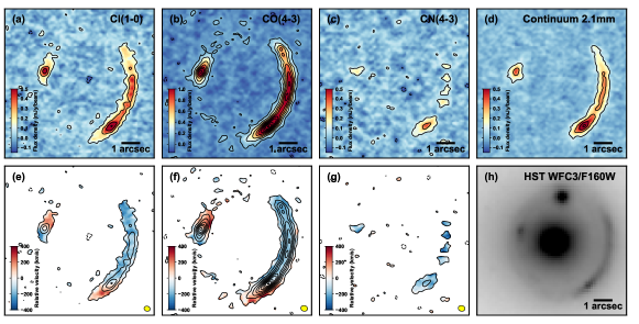
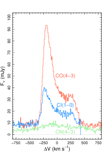
Figure 1.— ALMA observations of 9io9. Panels (a–c) show the velocity-averaged continuum-subtracted Ci.$(J=1\rightarrow 0)$, CO.$(J=4\rightarrow 3)$ and CN.$(N=4\rightarrow 3)$ maps respectively, and panel (d) shows the 2.1 mm continuum. In panels (a–d) contours start at 100 $\mu$Jy beam^-1 and increase in steps of 200 $\mu$Jy beam^-1. Panels (e–g) show the Ci.$(J=1\rightarrow 0)$, CO.$(J=4\rightarrow 3)$ and CN.$(N=4\rightarrow 3)$ velocity fields derived from the 1st moment maps, where the blue-to-red color scale spans $-400<\Delta V<400$ km s^-1 (black contours are the flux density contours in (a–c). The yellow ellipse indicates the size and shape of the synthesized beam. Panel (h) shows the archival Hubble Space Telescope 1600 nm (WFC3/F160W) image of the target (data acquired from The Mikulski Archive for Space Telescopes, proposal ID 14653), showing the partial Einstein ring of the background galaxy and the two foreground lensing galaxies: a $z\approx 0.2$ elliptical and a smaller northern companion, which has similar color and is assumed to be at the same redshift. All images are orientated north up, east left. The plot on the right shows the galaxy-integrated Ci.$(J=1\rightarrow 0)$, CO.$(J=4\rightarrow 3)$ and CN.$(N=4\rightarrow 3)$ spectra, including continuum contribution. The asymmetric double horned profile of Ci.$(J=1\rightarrow 0)$ & CO.$(J=4\rightarrow 3)$ are consistent with the lower spectral resolution observations of CO.$(J=3\rightarrow 2)$ in 9io9 by Harrington et al. (2016).

2. Observations

9io9 (02^h09^m41.3^s, +00^∘15^′58.5^′′) was observed with the ALMA 12 m array on 11^th and 14^th December 2017 in two 53 minute execution blocks as part of project 2017.1.00814.S. The representative frequency of the tuning was 139.2 GHz in Band 4, with central frequencies of the four spectral windows 127.196, 129.071, 139.196, 141.071 GHz. The correlator was set up in Frequency Division Mode with 480 channels per 1.875 GHz-wide baseband with a total bandwidth of 3.6 GHz, recording dual linear polarizations. Calibrators included J0238$+$1636 and J0208$-$0047. Observations were designed to cover the redshifted emission lines of the atomic carbon ${}^{3}P_{1}\rightarrow\phantom{}^{3}P_{0}$ fine structure line Ci.$(J=1\rightarrow 0)$ ($\nu_{\rm rest}=492$ GHz) and carbon monoxide CO.$(J=4\rightarrow 3)$ ($\nu_{\rm rest}=461$ GHz), but the bandwidth also covers hydrogen isocyanide HNC.$(J=5\rightarrow 4)$ ($\nu_{\rm rest}=453.270$ GHz) and the cyanide radical, CN.$(N=4\rightarrow 3)$. The latter comprises 19 hyperfine structure components, distributed in the three main fine structure spin groups: $J=7/2\rightarrow 7/2$, $J=7/2\rightarrow 5/2$, $J=9/2\rightarrow 7/2$ (at $\nu_{\rm rest}\approx\,452.628$, 453.389, and 453.606 GHz respectively). The relative intensities of these three groups is approximately 0.08:0.9:1, thus the $J=7/2\rightarrow 7/2$ component has a negligible contribution.

After two executions that built up 1.8 hours on-source integration, we reached a 1$\sigma$ (rms) sensitivity of 150 $\mu$Jy per 23 MHz (50 km s^-1) channel. The array was in configuration C43–6 with maximum baselines $\sim$3000 m, giving a synthesized beam $0.27^{\prime\prime}\times 0.21^{\prime\prime}$ at a position angle of 88 degrees. We make use of the ALMA Science Pipeline produced calibrated measurement set, and image the visibilities using the casa (v.5.1.0-74.el7) clean task, employing multiscale (scales of 0^′′, 0.5^′′ and 1.25^′′) and cleaning in frequency mode. We clean down to a stopping threshold of 1$\sigma$, and use natural weighting in the imaging.

Figure 1 presents the observations. We detect thermal dust continuum emission, the Ci.$(J=1\rightarrow 0)$ and CO.$(J=4\rightarrow 3)$ emission lines, and a weaker broad emission feature at $\nu_{\rm obs}\approx 127.6$ GHz which is a blend of HNC.$(J=5\rightarrow 4)$ and CN.$(N=4\rightarrow 3)$ that we show in Section 4.2 is dominated by the latter. The Ci.$(J=1\rightarrow 0)$ and CO.$(J=4\rightarrow 3)$ lines exhibit a classic double horn profile indicative of a rotational ring or disc (e.g. Downes & Solomon 1998), and with a distinctive shear in the velocity fields, we can spatially resolve the kinematics of the molecular gas.

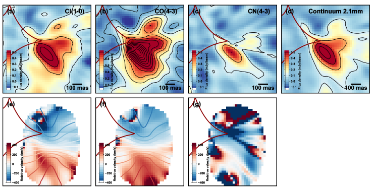
Figure 2.— Source plane reconstruction of Ci.$(J=1\rightarrow 0)$, CO.$(J=4\rightarrow 3)$ and CN.$(N=4\rightarrow 3)$ line emission in 9io9. Panels (a–g) show the equivalent maps as those displayed in Figure 1 for the image plan, with identical flux density contours. In panels (e & f) we show the velocity field from our rotating ring model (Section 3.2) as contours, spanning $-350$–$350$ km s^-1 in steps of $50$ km s^-1. CN.$(N=4\rightarrow 3)$ does not exhibit a coherent velocity field and is largely unresolved. Red solid lines show the lensing caustic from our best fitting lens model (Section 3.2).

3. Analysis

3.1. Basic properties

The sharp truncation of the CO.$(J=4\rightarrow 3)$ and Ci.$(J=1\rightarrow 0)$ lines characteristic of the double horn profile allow us to revise the redshift of 9io9. We find the best-fitting redshift that puts the mid-point of the full width at zero intensity (fwzi $=800$ km s^-1) of the continuum-subtracted lines at zero relative velocity, with $z=2.5543\pm 0.0002$. This is slightly higher than the value of $z=2.553$ reported by Geach et al. (2015) and Harrington et al. (2016), but we note that the coarse velocity resolution of these previous observations might have slightly biased the redshift estimate given the asymmetric nature of the CO.$(J=4\rightarrow 3)$ and Ci.$(J=1\rightarrow 0)$ lines.

We evaluate total line luminosities of a particular species, $x$ in standard radio units as

$$\frac{L^{\prime}_{x}}{{\rm K\,km\,s^{-1}\,pc^{2}}}=\left(\frac{3.25\times 10^{7}}{1+z}\right)\left(\frac{D_{l}}{{\rm Mpc}}\right)^{2}\\ \times\left(\frac{\nu_{\rm x,rest}}{\rm GHz}\right)^{-2}\left(\frac{\int S_{\nu}dV}{\rm Jy\,km\,s^{-1}}\right),$$ (1)

where $D_{l}$ is the luminosity distance, $\nu_{\rm x,rest}$ is the rest frame frequency of the line and $\int S_{\nu}dV$ is the velocity-integrated line flux. To evaluate $\int S_{\nu}dV$ for a transition $x$ we sum over the solid angle subtended by the region defined by the $\geq$3$\sigma$ contour in the velocity-averaged line maps, integrated over $|\Delta V|<500$ km s^-1. The uncertainty on integrated flux (and luminosity) values is determined by adding Gaussian noise to each channel, randomly drawn from off-line frequency ranges of the data cube (after continuum subtraction), where the scale is determined from the standard deviation of the flux density in equivalent contiguous solid angle in randomly chosen source-free parts of the data cube. By repeating this process 1000 times we asses the standard deviation in $\int S_{\nu}dV$ and derived luminosity, which we take as the 1$\sigma$ uncertainty. The source integrated flux of the CO.$(J=4\rightarrow 3)$ and Ci.$(J=1\rightarrow 0)$ lines are $S\Delta V=25.9\pm 0.2$ Jy km s^-1 and $S\Delta V=9.5\pm 0.1$ Jy km s^-1, corresponding to luminosities of $\mu L^{\prime}=(50.9\pm 0.3)\times 10^{10}$ K km s^-1 pc² and $\mu L^{\prime}=(16.4\pm 0.2)\times 10^{10}$ K km s^-1 pc², where $\mu$ is the lensing magnification. We discuss the lens model in the next section, and the HNC.$(J=5\rightarrow 4)$/CN.$(N=4\rightarrow 3)$ blend in Section 4.2.

3.2. Lens modelling

The lens model accommodates the gravitational potential of both the primary lensing galaxy ($z\approx 0.2$) and its smaller northern companion (Geach et al. 2015, Figure 1). We use a semi-linear inversion method (Warren & Dye 2003; Dye et al. 2018) to reconstruct a pixelized map of source surface brightness that best fits the observed lensed image for a given lens model. The lens model is iterated, reconstructing the source with each iteration, until the global best fit has been obtained according to the Bayesian evidence (Suyu et al. 2006). The lens mass model is motivated by the observed lens galaxy light; for the primary lens we use an elliptical power-law surface mass density profile of the form

$$\kappa=\kappa_{0}\,({\tilde{r}}/{\rm 1kpc})^{1-\alpha}\,,$$ (2)

where $\kappa_{0}$ is the normalisation surface mass density and $\alpha$ is the power-law index of the volume mass density profile. Here, the elliptical radius ${\tilde{r}}$ is defined by ${\tilde{r}}^{2}=x^{\prime 2}+y^{\prime 2}/\epsilon^{2}$ where $\epsilon$ is the lens elongation (i.e. the ratio of semi-major to semi-minor axis length) and the co-ordinate $(x,y)$ is measured with respect to the lens centre of mass located at $(x_{c},y_{c})$. The orientation of the semi-major axis measured counter-clockwise from north is described by the parameter $\theta$. Since the lensing effect by the secondary galaxy on the observed image is expected to be relatively minor (because, for realistic mass-to-light ratios, its lower observed flux implies low mass and because the influence of the secondary mass is largely where there is no observed Einstein ring flux) and to avoid over-complicating the lens model, for the companion lensing galaxy we assume a singular isothermal sphere profile fixed at the observed galaxy light centroid with a surface mass density of the form

$$\kappa(r)=\kappa_{0s}\frac{r_{0}}{r}\,.$$ (3)

Here, $\kappa_{0s}$ is the normalisation surface mass density and $r_{0}$ is a constant set to 1 kpc. The lens model also includes an external shear field characterised by the shear strength, $\gamma$, and the shear direction angle $\theta_{\gamma}$.

The set of parameters is optimized using the Markov Chain Monte Carlo (MCMC) method (Suyu et al. 2006) using as input the velocity-integrated, cleaned CO.$(J=4\rightarrow 3)$ emission. To eliminate possible biases in the optimization, we apply the random Voronoi source plane pixelization method (Dye et al. 2018). This optimal lens model is then subsequently used to reconstruct the source plane emission on a regular pixel grid in each observed channel to produce a source plane data cube covering the full observed frequency range.

We find a best fitting density profile for the primary lens that is nearly isothermal with $\alpha=2.03$, an ellipticity of $\epsilon=0.12$ and semi-major axis orientation of $\theta=93^{\circ}$ east of north which aligns closely with the observed lens galaxy light. The model returns a total mass-to-light ratio for the secondary lens that is 0.65$\times$ that of the primary, assuming that both lie at the same redshift. Our lens model also includes external shear to accommodate weaker deflections caused by the combination of possible mass external to the primary and secondary lens system. The fit is improved significantly with a shear of $\gamma=0.05$ orientated such that the direction of stretch is $\theta_{\gamma}=20^{\circ}$ west of north. The fwhm of the minor axis of the effective beam in the source plane is 45 mas, corresponding to a physical (projected) scale of 360 pc. Figure 2 shows the source plane reconstructions of the velocity-integrated emission line maps and velocity fields. The total magnification is $\mu=14.7\pm 0.3$, and generally the lens model is similar the one presented in Geach et al. (2015). In the following, all derived physical properties are in the $z=2.6$ source plane, and we perform the analysis in the source plane-reconstructed data cubes, thus taking into account differential lensing.

3.3. Dynamical modelling

We use the code galpak3d (Bouché et al. 2015) (version 1.8.8) to fit the source plane CO.$(J=4\rightarrow 3)$ data cube with a rotating ring/disk model. We make a slight modification to the publicly available code to allow an additional definition for the density distribution, observed in local ultraluminous infrared galaxies (Downes & Solomon 1998):

$$n(R)=n_{0}\exp\left[4A\ln{2}\left(\frac{R-R_{\rm min}}{\Delta R}\right)^{2}\right]+n_{0}R^{\alpha},$$ (4)

where $n_{0}$ and $A$ are normalisation constants, $R_{\rm min}$ is the inner edge of the ring (with $R_{\rm min}=0$ defining a disk), and $R_{\rm max}$ is the outer edge (with $n(R>R_{\rm max})=0$). As in previous works, we fix $\alpha=0$, but $A$ is allowed as a free parameter, as are $n_{0}$, $R_{\rm min}$, $R_{\rm max}$ and $\Delta R$. Perpendicular to the disc we assume a Gaussian flux profile (Bouché et al. 2015) The total velocity dispersion of the disc is assumed to be a quadrature sum of (a) the local isotropic velocity dispersion from self-gravity, (b) a term due to mixing of velocities along the line-of-sight, and (c) an intrinsic dispersion term (a free parameter) that accounts for (e.g.) turbulent gas motions. Finally, we adopt a hyperbolic tangent rotation curve:

$$V(R)=V_{\rm max}\tanh(R/R_{V}),$$ (5)

where $R_{V}$ is the turnover radius, with $V_{\rm max}$ and $R_{V}$ free parameters (Andersen & Bershady 2013). Since the effective beam size varies over the field-of-view in the reconstructed data cube, we convolve each channel in the input CO.$(J=4\rightarrow 3)$ cube with a circular Gaussian PSF with a width that aims to homogenise the angular resolution across the source plane. We fix the fwhm of this kernel as the $\theta=135$ mas which is the effective beam size at the centre of the source plane.

We experiment with a set of several different starting parameter values and maximum iterations to determine a ‘first guess’ solution that reasonably fits the data. To refine the fit, and to explore the sensitivity of chain convergence to starting values, we take this first set of parameters as nominal starting values, and run 1000 independent chains, each with a maximum of 5000 iterations. In each run, we perturb each parameter by sampling from a Gaussian distribution centred at the nominal value with a standard deviation set at 10% of the magnitude of the central value. We find consistent chain convergence, with a median reduced $\chi^{2}=1.08$. Taking the distribution of converged $\chi^{2}$ values over all 1000 chains, the 1st and 99th percentiles are $\chi^{2}=0.99$ and $\chi^{2}=1.23$ respectively. We take the 50th percentile of the converged parameters over the 1000 chains as the final estimate of the best-fitting model parameters, and the 16th and 84th percentiles as the 1$\sigma$ uncertainty bounds. The best-fitting model has $R_{\rm min}=20^{+12}_{-2}$ mas ($161^{+102}_{-18}$ pc), $R_{\rm max}=322^{+11}_{-20}$ mas ($2647^{+88}_{-160}$ pc), $i=50^{+3}_{-8}$ degrees, $\Delta R=75^{+14}_{-13}$ mas ($613^{+111}_{-110}$ pc), $\theta=5\pm 4$ degrees, $V_{\rm max}=360^{+49}_{-11}$ km s^-1, $\sigma_{\rm disk}=73\pm 4$ km s^-1. Figure 3 compares this model to the data.

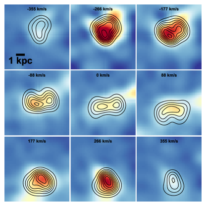
Figure 3.— Dynamical modelling of 9io9. We show the source plane CO.$(J=4\rightarrow 3)$ emission averaged over 88 km s^-1-wide channels spanning $-350$–$350$ km s^-1. The color scale saturates at 4 mJy. Contours show the equivalent line emission extracted from the best-fitting model data cube, describing a rotating ring with inner radius 160 pc, outer radius approximately 2.5 kpc and maximum deprojected velocity 360 km s^-1. Contours show the corresponding emission in the model cube, starting at 0.5 mJy and increasing in steps of 0.5 mJy.

3.4. Molecular gas mass

We measure the intrinsic (i.e. source plane) line luminosities as $L^{\prime}_{\rm CI}=(8.7\pm 0.1)\times 10^{9}$ K km s^-1 pc² and $L^{\prime}_{\rm CO}=(32.3\pm 0.2)\times 10^{9}$ K km s^-1 pc². To evaluate the molecular hydrogen mass from the atomic carbon line luminosity we follow previous works (Weiß et al. 2003; Papadopoulos et al. 2004; Papadopoulos & Greve 2004; Wagg et al. 2006; Alaghband-Zadeh et al. 2013; Bothwell et al. 2017)

$$\frac{M_{\rm H_{2}}}{M_{\odot}}=\left(\frac{1376}{1+z}\right)\left(\frac{D_{l}}{\rm Mpc}\right)^{2}\left(\frac{X_{\rm CI}}{10^{-5}}\right)^{-1}\\ \times\left(\frac{A_{10}}{10^{-7}{\rm s^{-1}}}\right)^{-1}Q^{-1}_{10}\left(\frac{S_{\rm CI}}{{\rm Jy\,km\,s^{-1}}}\right),$$ (6)

where $X_{\rm CI}$ is the atomic carbon to molecular hydrogen abundance ratio, $A_{10}$ is the Einstein $A$-coefficient for the Ci.$(J=1\rightarrow 0)$ transition ($A_{10}=7.93\times 10^{-8}$ s^-1) and $Q_{10}$ is the excitation factor defined by the ratio of the column density of the upper excited level $(^{3}P_{1})$ to the ground state (${}^{3}P_{0}$). This depends on the density and kinetic temperature of the gas, which are not well constrained, but as in other works we assume a Ci/H₂ abundance $X_{\rm CI}=3\times 10^{-5}$ and excitation $Q_{10}=0.5$ (Papadopoulos & Greve 2004). This gives $M_{\rm H_{2}}=(7.5\pm 0.1)\times 10^{10}M_{\odot}$. Recently, Rivera et al. (2018) presented an analysis of the CO.$(J=3\rightarrow 2)$ map of 9io9 at approximately 1^′′ resolution, deriving a slightly lower $M_{\rm H_{2}}=(3.5\pm 0.2)\times 10^{10}M_{\odot}$, however systematic uncertainties on $\alpha_{\rm CO}$ and lensing magnification could easily bring the values into parity.

4. Interpretation

4.1. The molecular ring

The total mass within $R_{\rm max}$ can be estimated from the dynamical mass, $M_{\rm dyn}=V_{\rm max}^{2}R_{\rm max}/G$, with the model giving $M_{\rm dyn}=(8.1^{+1.5}_{-0.8})\times 10^{10}M_{\odot}$. This indicates that the potential within 2.5 kpc of the SMBH is molecular gas-dominated. The line ratio $L^{\prime}_{\rm CO(4-3)}/L^{\prime}_{\rm CI}$ can further inform us about the conditions of the gas in the ring, since it is sensitive to the the dense-to-total molecular gas ratio $f_{d/t}$, in turn thought to be a reliable indicator of the star formation efficiency (Papadopoulos & Geach 2012). For example, $L^{\prime}_{\rm CO(4-3)}/L^{\prime}_{\rm CI}$ can vary by an order of magnitude between different star-forming environments, with values of $\sim$0.5 for quiescent disks and clouds in the Milky Way and local Universe, up to $\sim$5 for galactic nuclei, ultraluminous infrared galaxies and quasars (e.g. Israel et al. 1995, 1998; Barvainis et al. 1997; Petitpas & Wilson 1998; Israel & Baas 2001, 2003; Papadopoulos & Greve 2004; Papadopoulos et al. 2004).

We measure $L^{\prime}_{\rm CO(4-3)}/L^{\prime}_{\rm CI}=3.7\pm 0.1$, indicating $f_{d/t}\sim 0.5$ (Papadopoulos & Geach 2012). From this we can estimate the total star formation rate by assuming the total molecular gas mass is related to on-going star formation as $\psi_{\star}=\epsilon f_{d/t}M_{\rm H_{2}}$. The factor $\epsilon$ describes the star formation efficiency of dense molecular gas, with compelling observational evidence that $\epsilon$ is roughly constant, possibly reflecting a local efficiency at the fundamental scale of star formation (Thompson et al. 2005). Expressed in terms of the emergent infrared luminosity, $\epsilon=500\,(L_{\odot}/M_{\odot})$ (Shirley et al. 2003; Scoville et al. 2004), we estimate the total star formation rate in the molecular ring as $\psi_{\star}\approx 2800$ $M_{\odot}$ yr^-1, modulo systematic uncertainties on the form of the stellar initial mass function, (e.g. Zhang et al. 2018).

4.2. A possible dense molecular outflow

The broad emission feature at $\nu_{\rm obs}=127.6$ GHz is a blend of HNC.$(J=5\rightarrow 4)$ and CN.$(N=4\rightarrow 3)$. The velocity-integrated emission is more compact than the CO.$(J=4\rightarrow 3)$ and Ci.$(J=1\rightarrow 0)$ in the source plane (Figure 2), with approximately 80% of the integrated flux unresolved, corresponding to emission on scales below 360 pc. To model this feature we assume that both HNC.$(J=5\rightarrow 4)$ and CN.$(N=4\rightarrow 3)$ contribute to the observed emission line, and, since they trace similar gas densities ($n\sim 10^{5-6}$ cm^-3), assume that both lines are kinematically broadened by the same Gaussian $\sigma_{\rm dense}$.

For the CN.$(N=4\rightarrow 3)$ line, with its various fine- and hyperfine structure components, we assume local thermodynamic equilibrium and optically thin emission, adopting the relative line intensities from the Cologne Database for Molecular Spectroscopy (Muller et al. 2005), calculated at 300 K (since we have no reliable estimate of the temperature). We fit the spectrum allowing the HNC.$(J=5\rightarrow 4)$ and CN.$(N=4\rightarrow 3)$ amplitudes, $\sigma_{\rm dense}$ and redshift (assuming the same for both species) to vary as free parameters. We also allow for a constant amplitude continuum. The best fitting redshift is $z=2.5543\pm 0.0005$, consistent with the value reported in Section 3.1.

The data and best fitting model are shown in Figure 4, where we find that the observed emission is dominated by CN.$(N=4\rightarrow 3)$ with a statistically insignificant HNC.$(J=5\rightarrow 4)$ contribution. Interestingly, the opposite was found for APM 08279$+$5255 ($z=4$) by Guélin et al. (2007), who found a line blend dominated by HNC.$(J=5\rightarrow 4)$, with $L^{\prime}_{\rm HNC}/L^{\prime}_{\rm CN}\approx 2$, although CN.$(N=4\rightarrow 3)$ is only tentatively detected in that system. However, we caution the reader that the deblending is highly dependent on redshift. For example, fixing $z=2.5534$ (e.g. Harrington et al. 2016) results in a more substantial HNC.$(J=5\rightarrow 4)$ contribution to the blend. Since internal motions/offsets of order 100 km s^-1 (relative to the molecular ring) for the dense gas traced by HNC.$(J=5\rightarrow 4)$ and CN.$(N=4\rightarrow 3)$ are possible, we are reticent in drawing any conclusions regarding the relative strengths of these lines; deeper observations will be required to properly model the complex, ideally with coverage of other dense gas tracers to properly constrain the physical conditions. Regardless of this, it is clear that one, or both, of the lines must be very broad, and this might provide clues as to the nature of the very dense gas in 9io9 compared to the molecular ring.

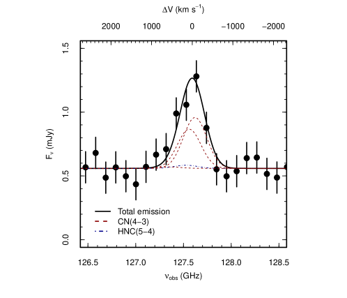
Figure 4.— Detection of CN.$(N=4\rightarrow 3)$. The observed spectrum at 126.5–128.5 GHz is modelled with a combination of HNC.$(J=5\rightarrow 4)$ and CN.$(N=4\rightarrow 3)$ gaussian emission lines with fixed redshift and velocity dispersion, plus a constant continuum component. CN.$(N=4\rightarrow 3)$ comprises 19 hyperfine components in three spin groups, with the $J=7/2\rightarrow 5/2$ and $J=9/2\rightarrow 7/2$ components dominating the CN.$(N=4\rightarrow 3)$ total emission for relative intensities calculated assuming optically thin conditions and local thermodynamic equilibrium (Muller et al. 2005). Our best-fitting model shows a negligible contribution from HNC.$(J=5\rightarrow 4)$ (although we caution against drawing any conclusions regarding the relative strength of the lines, see Section 4.2), and supports a broad velocity width of fwhm $=680$ km s^-1. Note, for presentation, the data has been binned to a channel width of 100 MHz or 240 km s^-1, but the fit was done on the full resolution spectrum.

The model line width is $\sigma_{\rm dense}=(289\pm 48)$ km s^-1, corresponding to a fwhm $\approx 680$ km s^-1, nearly a factor of two larger than the deprojected maximum rotation speed of the molecular ring. Note that fixing the velocity width of the HNC.$(J=5\rightarrow 4)$ and CN.$(N=4\rightarrow 3)$ components to the $\sigma_{\rm disk}=73$ km s^-1 dispersion of the molecular ring does not result in a sensible fit to the data. The compact nature of the CN.$(N=4\rightarrow 3)$ emission compared to Ci.$(J=1\rightarrow 0)$ and CO.$(J=4\rightarrow 3)$, coupled with its large velocity width compared to the deprojected rotation speed of the ring, suggests that the gas traced by CN.$(N=4\rightarrow 3)$ does not trace the bulk of the gas reservoir and could be dynamically decoupled from the ring.

5. Conclusion

One interpretation of these observations is that the gas traced by CN.$(N=4\rightarrow 3)$ is outflowing, potentially indicating interaction between the AGN and the inner part of the molecular ring or smaller scale circumnuclear disk. However, we note that the high star formation rate density of the ring could also be conducive to the formation and excitation of CN (although in that case the broad line would likely have to be produced by a supernova-driven wind; not implausible given the high $\psi_{\star}$). With the current data (i.e. the lack of a broader range of tracers) we cannot unambiguously distinguish between an AGN versus ‘star formation’ origin of the CN.$(N=4\rightarrow 3)$ emission; indeed the interpretation of this species in general is rather complex (Meijerink & Spaans 2005, Wilson 2018). Nevertheless, CN can be produced through the photodissociation of species such as HCN and its isomers in environments with intense ultraviolet or X-ray radiation fields (Fuente et al. 1993; Rodriguez-Franco et al. 1998; Meijerink & Spaans 2005; Meijerink et al. 2007) as exists around AGN (Aalto et al. 2002; Chung et al. 2011).

Given the prevalence of molecular outflows on similar scales in local ULIRGs (e.g. Feruglio et al. 2010; Sturm et al. 2011; Cicone et al. 2014), the presence of a dense molecular outflow in 9io9 is not surprising. Perhaps more surprising is the realisation that AGN feedback will do little to curtail the ongoing rapid stellar mass assembly in the surrounding ring, given the short gas consumption timescale due to star formation, $M_{\rm H_{2}}/{\psi}_{\star}\sim 10$s Myr. We cannot yet estimate the mass outflow rate in the putative molecular wind, but it is clear that it cannot represent a significant fraction of the total gas reservoir. Thus, gas exhaustion, rather than quenching, will result in 9io9 transitioning into a passive elliptical galaxy. This is not to say that the AGN will not play a regulatory role in future stellar mass growth, but these observations suggest that co-eval radio-mode AGN feedback could be extraneous to the rapid assembly of stellar bulges at the peak epoch of galaxy formation.

References

- Aalto (2002) Aalto, S., et al. 2002, A&A, 381, 783
- Alaghband-Zadeh (2013) Alaghband-Zadeh, S., et al. 2013, MNRAS, 435, 1493
- Andersen (2013) Andersen, D. R. & Bershady, M. A. 2013, ApJ, 768, 41
- Annis (2014) Annis, J., et al. 2014, ApJ, 794, 120
- Barvainis (1997) Barvainis, R., et al. 1997, ApJ, 484, 695
- Biernacki (2018) Biernacki, P. & Teyssier, R. 2018, MNRAS, 475, 5688
- Bothwell (2017) Bothwell, M. S., et al. 2017, MNRAS, 466, 2825
- Bouche (2015) Bouché, N., et al. 2015, AJ, 150, 92
- Bower (2006) Bower, R. G., et al. 2006, MNRAS, 370, 645
- Chung (2011) Chung, A., et al. 2011, ApJ, 732, L15
- Cicone (2014) Cicone, C., et al. 2014, A&A, 562, A21
- Cicone (2015) Cicone, C., et al. 2015, A&A, 574, A14
- Croton (2006) Croton, D. J., et al. 2006, MNRAS, 365, 11
- DiMatteo (2005) Di Matteo, T., et al. 2005, Nature, 433, 604
- Downes (1998) Downes, D. & Solomon, P. M. 1998, ApJ, 507, 615
- Dye (2018) Dye, S. et al., 2018, MNRAS, 476, 4383
- Erben (2013) Erben, T., et al. 2013, MNRAS, 433, 2545
- Fabian (2012) Fabian, A. C. 2012, ARA&A, 50,455
- Faucher-Giguere (2012) Faucher-Giguére, C.-A. & Quataert, E. 2012, MNRAS, 425, 605
- Feruglio (2010) Feruglio, C. et al. 2010, A&A, 518, L155
- Fuente (1993) Fuente, A., et al. 1993, A&A, 276, 473
- Geach (2015) Geach, J. E., et al. 2015, MNRAS, 452, 502
- Geach (2017) Geach, J. E., et al. 2017, ApJS, 231, 7
- Granato (2004) Granato, G. L., et al. 2004, ApJ, 600, 580
- Guelin (2007) Guélin, M. et al. 2007, A&A, 462, L45
- Harrington (2016) Harrington, K. C., et al. 2016, MNRAS, 458, 4383
- Hopkins (2010) Hopkins, P. F. & Elvis, M. 2010, MNRAS, 401, 7
- Isreal (1995) Israel, F. P., et al. 1995, A&A, 302, 343
- Isreal (1998) Israel, F. P., et al. 1998, A&A, 339, 398
- Isreal (2001) Israel, F. P. & Baas, F. 2001, A&A, 371, 433
- Isreal (2003) Israel, F. P. & Baas, F. 2003, A&A, 404, 495
- Ivison (2010) Ivison, R. J., et al. 2010, MNRAS, 402, 245
- King (2015) King, A. & Pounds, K. 2015, ARA&A, 53, 115
- Madau (2014) Madau, P. & Dickinson, M. 2014, ARA&A, 52, 415
- Marshall (2016) Marshall, P. J., et al. 2016, MNRAS, 455, 1171
- Meijerink (2005) Meijerink, R., Spaans, M. 2005, A&A, 436, 397
- Meijerink (2007) Meijerink, R., et al. 2007, A&A, 461, 793
- More (2016) More, A., et al. 2016, MNRAS, 455, 1191
- Muller (2005) Müller, H. S. P., et al. 2005, Journal of Molecular Structure, 742, 215
- Negrello (2010) Negrello, M., et al. 2010, Science, 330, 800
- Papadopoulos (2004a) Papadopoulos, P. P., et al. 2004, MNRAS, 351, 147
- Papadopoulos (2004) Papadopoulos, P. P. & Greve, T. R. 2004, ApJ, 615, L29
- Papadopoulos (2012) Papadopoulos, P. P. & Geach, J. E. 2012, ApJ, 757, 157
- Petitpas (1998) Petitpas, G. R. & Wilson, C. D. 1998, ApJ, 503, 219
- Planck (2015) Planck Collaboration 2015, A&A, 594, A13
- Rodriguez-Franco (1998) Rodriguez-Franco, A., et al. 1998, A&A, 329, 1097
- Scoville (2004) Scoville, N. 2004, A&A, 320, 253
- Shirley (2003) Shirley, Y. L., et al. 2003, ApJS, 149, 375
- Silk (1998) Silk, J. & Rees, M. J. 1998, A&A, 331, L1
- Sturm (2011) Sturm, E. et al., 2011, ApJ, 733, L16
- Suyu (2006) Suyu, S. H. et al., 2006, MNRAS, 371, 983
- Thompson (2005) Thompson, T. A., et al. 2005, ApJ, 630, 167
- Tombesi (2015) Tombesi, F., et al. 2015, Nature, 519, 436
- Veilleux (2017) Veilleux, S., et al. 2017, ApJ, 843, 18
- Wagg (2006) Wagg, J., et al. 2006, ApJ, 651, 46
- Warren (2003) Warren, S. J. & Dye, S. 2003, ApJ, 590, 673
- Weiss (2003) Weiß, A., et al. 2003, A&A, 409, L41
- Wilson (2018) Wilson, C. D. 2018, MNRAS, 477, 2926
- Zhang (2018) Zhang, Z-Y., et al. 2018, Nature, 558, 260