Recurrence and windings of two revolving random walks

Abstract

We study the winding behavior of random walks on two oriented square lattices. One common feature of these walks is that they are bound to revolve clockwise. We also obtain quantitative results of transience/recurrence for each walk.

Keywords: winding, oriented lattices, transience/recurrence, Lyapunov function.
Mathematics Subject Classification 2010: Primary 60G50; Secondary 60J10.

1 Introduction

(a) Graph $\mathbb{G}_{1}$

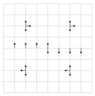
(b) Graph $\mathbb{G}_{2}$

Figure 1: The graph $\mathbb{G}_{1}$ in figure (a) is transient, whereas the graph $\mathbb{G}_{2}$ in (b) is recurrent. The arrows indicate the orientation of the corresponding edges.

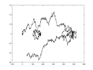
(a) Random walk on $\mathbb{G}_{1}$

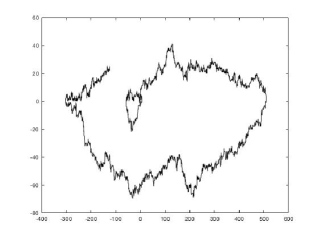
(b) Random walk on $\mathbb{G}_{2}$

Figure 2: Simulated trajectories of 5000 steps of the random walks on $\mathbb{G}_{1}$ and $\mathbb{G}_{2}$. Note the different scaling of the axes.

Spitzer’s celebrated theorem [35] states that the winding angle of a planar Brownian motion up to time $t$, rescaled by $\frac{1}{2}\log t$, has standard Cauchy as its limiting distribution. Since then, the winding behavior of planar processes has attracted the interest of many researchers. For the 2D simple random walk, Bélisle [2] showed that its winding angle has the same scaling limit as the big winding angle of a 2D Brownian motion, that is, the winding angle taking place outside a small ball centered at the origin. The latter is determined to be asymptotically hyperbolic secant with density $(1/2)\text{sech}(\pi u/2)$ in [27, 31]. We refer to [3] for a detailed review on this topic. See also [34, 33, 7].

In a different direction, the study of random walks on oriented lattices has intensified in the last few decades with motivations from many sources, including the Matheron-de Marsily model of transport in porous media [24], discretized gauge theories [8, 9] and the theory of random walks in random media [18]. Various aspects of these models are studied (e.g. [17, 11], [16, 28, 10]) with many extensions [12, 6, 23] and connections to other models [26, 25, 29]. Except in special cases, random walks on oriented lattices are non-reversible and non-elliptic, which poses a unique set of challenges for analysis.

In this paper we study the winding behavior of the random walks on two oriented lattices $\mathbb{G}_{1}$ and $\mathbb{G}_{2}$, illustrated in Figure 1. This is of particular interest, as both random walks are bound to revolve clockwise around the origin. After deducing the asymptotic laws of windings, we explain how these laws are closely related to more classical ones, such as the Spitzer’s law. For each walk, we also derive quantitative results of transience or recurrence through our understanding of the windings.

1.1 Models and results

We give the precise definitions of $\mathbb{G}_{1}$ and $\mathbb{G}_{2}$. Define the directed graph $\mathbb{G}_{1}=(\mathbb{Z}^{2},\mathbb{E}_{1})$ such that a directed edge $(v,w)=((v_{1},v_{2}),(w_{1},w_{2}))\in\mathbb{E}_{1}$ if and only if $(w_{1},w_{2})=(v_{1},v_{2}\pm 1)$, or $(w_{1},w_{2})=(v_{1}+1,v_{2})$ and $v_{2}=w_{2}\geq 0$, or $(w_{1},w_{2})=(v_{1}-1,v_{2})$ and $v_{2}=w_{2}<0$. The graph $\mathbb{G}_{2}=(\mathbb{V},\mathbb{E}_{2})$ can be obtained with a slight modification of $\mathbb{G}_{1}$ by redefining only the orientations of the edges leading out from $x$-axis, that is, $((v_{1},0),(w_{1},w_{2}))\in\mathbb{E}_{2}$ with $v_{1}=w_{1}$ and $w_{2}=\pm 1$ if and only if $w_{2}=-1$ and $v_{1}=w_{1}>0$, or $w_{2}=1$ and $v_{1}=w_{1}<0$, or $w_{2}=\pm 1$ and $v_{1}=w_{1}=0$.

Although $\mathbb{G}_{1}$ and $\mathbb{G}_{2}$ may look very similar, the random walks on them exhibit completely different behaviors. The graph $\mathbb{G}_{1}$ appeared for the first time in [8], where a proof of transience was given; the graph $\mathbb{G}_{2}$ was introduced later in [26, 25] and the random walk on it turns out to be recurrent. The recurrence of $\mathbb{G}_{2}$ follows from Corollary 4.8 in [20], as pointed out in [5, Prop. 7.8]. Both random walks, considered at their successive returns to the $x$-axis, belong to the class of 1D oscillating random walks [20, 26, 25], with $\mathbb{G}_{2}$ critically recurrent in the class.

Run a simple random walk on $\mathbb{G}_{1}$. Let $\mathcal{N}_{\mathbb{G}_{1}}(n)$ be the number of windings around the origin up to the $n$-th step. See (21) for the formal definition. Our first result is a strong LLN for $\mathcal{N}_{\mathbb{G}_{1}}(n)$.

Theorem 1.

$$\frac{\mathcal{N}_{\mathbb{G}_{1}}(n)}{\log n}\to\frac{1}{2\pi}\quad\text{a.s.}$$

Note that this is in sharp contrast with the winding angle of classical 2D Brownian motion and random walks, which have nontrivial scaling limits.

In order to prove Theorem 1, we obtain a local limit theorem for the return probabilities on $\mathbb{G}_{1}$. More precisely, let $(M_{i})_{i\geq 0}$ be the simple random walk on $\mathbb{G}_{1}$ and let $T_{n}$ be the time just after the $n$-th vertical step of $M$. Write $\mathbb{P}_{0}$ for the law of $(M_{i})_{i\geq 0}$ starting at the origin. Then we have the following precise asymptotics:

Theorem 2.

$$\mathbb{P}_{0}\left(M_{T_{2n}}=(0,0)\right)\sim\frac{1}{2\sqrt{\pi}n^{3/2}}.$$

Theorem 2, in turn, provides a new proof of the transience, see Corollary 10. In [11], similar results as Theorem 2 are obtained for random walks on randomly oriented lattices.

Now consider the simple random walk on $\mathbb{G}_{2}$. To study its winding, we will focus on a continuous-time process $(W_{t})_{t\geq 0}$ on $\mathbb{R}^{2}$, which is the scaling limit of the random walk on $\mathbb{G}_{2}$. Starting from the negative $x$-axis, the process $W_{t}$ drifts at unit speed to the right while performing a reflected Brownian motion vertically, until the first time it hits the positive $x$-axis, see Figure 3; then it continues analogously in the lower half plane but to the left until hitting the negative $x$-axis, and keeps alternating between two possibilities. A precise definition of $W_{t}$ is given in Section 3.1.

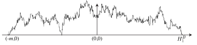
Figure 3: Illustration of the first step of the ladder height process.

Let $\mathcal{N}_{t}$ be the winding number of $W_{t}$ around the origin up to time $t$. As shown in [2], the big windings of a continuous process better capture the winding behavior of its discrete counterpart. So for $\epsilon>0$, also consider the big winding number $\mathcal{N}_{t}^{b}$ taking place outside a small ball of radius $\epsilon$ centered at the origin. The scaling limit in (2) below does not depend on the choice of $\epsilon$.

Theorem 3.

$$\frac{2\pi^{2}\mathcal{N}_{t}}{\log^{2}t}\overset{d}{\implies}\rho_{1}$$ (1)

and

$$\frac{2\pi^{2}\mathcal{N}_{t}^{b}}{\log^{2}t}\overset{d}{\implies}\int_{0}^{\rho_{1}}\mathbbm{1}_{\{\beta_{s}>0\}}ds$$ (2)

as $t\rightarrow\infty$. Here $\beta_{s}$ is a standard Brownian motion and $\rho_{h}$ represents its first hitting time at $h\in\mathbb{R}$.

Note that the limit in (2) has the same law as the hitting time of a reflected Brownian motion at one. So unlike the Lévy distribution (1), the distribution in (2) has sub-exponential tails. The comparison between (1) and (2) shows that it is the small windings near the origin that give the scaling limit of $\mathcal{N}_{t}$ its heavy tails. Similar comments were made about the planar Brownian motion in [3].

In particular, Theorem 3 shows that the winding and big winding numbers of $W_{t}$ grow faster than those of a planar Brownian motion. The difference results from the fact that $W_{t}$ is only allowed to wind in the clockwise direction, whereas the planar Brownian motion chooses both directions randomly. Surprisingly, the heuristic goes further by explaining the difference in scaling limits: the Cauchy and hyperbolic secant distributions have the same law as the Brownian motion subordinated to an independent random time distributed as (1) and (2) respectively. In other words, their scaling limits are off essentially by a central limit theorem. In the same spirit, Theorem 1 should be compared with the law in [4].

Our last result is about the tail of return time on $\mathbb{G}_{2}$, which quantifies its recurrence. For SRW on $\mathbb{Z}^{2}$, Dvoretzky and Erdös [14] showed that the return time to the origin has a tail of order $\Theta(1/\log k).$ By analyzing $W_{t}$ and exploiting the Lyapunov function methodology (see e.g. [25]), we are able to prove a similar tail bound for $\mathbb{G}_{2}$. Let $(X_{i},Y_{i})_{i\geq 0}$ be the simple random walk on $\mathbb{G}_{2}$. Define the return time $\tau_{0}^{+}:=\min\{i\geq 1;X_{i}=Y_{i}=0\}$.

Theorem 4.

$$\lim_{k\to\infty}\frac{\log\mathbb{P}_{0}(\tau_{0}^{+}>k)}{\log\log k}=-1.$$

In particular, this gives a new and self-contained proof of the recurrence of $\mathbb{G}_{2}$, see Sections 3.3 and 3.4.

1.2 Organization of the paper

In Section 2, we shall analyze $\mathbb{G}_{1}$ and prove Theorems 1 and 2. We introduce an auxiliary process $(\mathcal{G},S)$ in Section 2.1 and prove a strong LLN for its winding in Section 2.2. The auxiliary process $(\mathcal{G},S)$ mimics the behavior of the random walk on $\mathbb{G}_{1}$ but has cleaner algebra. We come back to $\mathbb{G}_{1}$ in Section 2.3, proving Theorem 2 as well as the transience of $\mathbb{G}_{1}$ in Corollary 10. Finally, in Section 2.4 we establish a comparison between the two processes and use the LLN for $(\mathcal{G},S)$ to deduce Theorem 1.

In Section 3, we shall study $\mathbb{G}_{2}$ and prove Theorems 3 and 4. We give a precise definition of the continuous process $W_{t}$ in Section 3.1 and prove Theorem 3 in Section 3.2. In Sections 3.3 and 3.4, we develop the key ingredients in the proof of Theorem 4 and prove the recurrence of $\mathbb{G}_{2}$ as an application. In Section 3.5 we prove Theorem 4. The most technical parts of the proofs are postponed to the appendices.

2 Random walk on $\mathbb{G}_{1}$

2.1 Auxiliary process $\mathcal{G}$

The main goal of Section 2 is to prove Theorem 1 for the random walk on $\mathbb{G}_{1}$. We start by introducing an analogous 2D process $(\mathcal{G},S)$ with nicer algebra.

Let $S$ be a simple random walk on $\mathbb{Z}$. Recall that the graph of such a random walk is given by the path successively connecting the sequence of vertices $\{(i,S_{i})\}_{i\geq 0}$ on $\mathbb{Z}^{2}$, with $e_{i}$ representing the line segment between $(i,S_{i})$ and $(i+1,S_{i+1})$. We define a signed time process

$$\mathcal{G}_{n}:=\sum_{i=0}^{n-1}\mathbf{1}_{\{e_{i}\text{ is above $x$-axis}\}}-\mathbf{1}_{\{e_{i}\text{ is below $x$-axis}\}}$$ (3)

to be the difference between the time spent above and below $x$-axis. Roughly speaking, the simple random walk $S$ corresponds to the vertical movement of the random walk on $\mathbb{G}_{1}$, whereas the signed time process $\mathcal{G}$ mimics the horizontal counterpart.

Let $\mathcal{N}_{\mathcal{G}}(n)$ be the number of windings around the origin of the two-dimensional process $(\mathcal{G},S)$ up to time $n$. We state an analogue of Theorem 1 for $\mathcal{N}_{\mathcal{G}}(n)$. Later in Section 2.4, we will establish a comparison between $\mathcal{N}_{\mathbb{G}_{1}}(n)$ and $\mathcal{N}_{\mathcal{G}}(n)$ and use Proposition 5 to prove Theorem 1. We will prove Proposition 5 in Section 2.2.

Proposition 5.

$$\frac{\mathcal{N}_{\mathcal{G}}(n)}{\log n}\to\frac{1}{2\pi}\quad\text{a.s.}$$

The following is a direct consequence of the usual Chung-Feller Theorem. See [19] for a general introduction on the topic.

Lemma 6.

For $z\in\{-2n,-(2n-4),\cdots,2n-4,2n\}$, we have

$$\mathbb{P}_{0}\left(\mathcal{G}_{2n}=z\mid S_{2n}=0\right)=\frac{1}{n+1}.$$ (4)

Thus for such $z$,

$$\mathbb{P}_{0}\left((\mathcal{G}_{2n},S_{2n})=(z,0)\right)\sim\frac{1}{\sqrt{\pi}n^{3/2}}.$$

The probabilities vanish for other $z$’s. ∎

2.2 Winding of the auxiliary walk

In this section we shall prove Proposition 5. We will use the following definition of $\mathcal{N}_{\mathcal{G}}(2n)$:

$$\mathcal{N}_{\mathcal{G}}(2n):=\frac{1}{2}\sum_{i=1}^{n}\mathbf{1}_{A_{2i}},$$

where for $i\in[1,n]$ we define $\tau_{i}:=\sup\{t<i;S_{2t}=0\}$ and

$$A_{2i}:=\{S_{2\tau_{i}}=S_{2i}=0\text{ and either }\mathcal{G}_{2\tau_{i}}\mathcal{G}_{2i}<0\text{ or }\mathcal{G}_{2\tau_{i}}=0\text{ and }\mathcal{G}_{2i}>0\}.$$

In words, we define $A_{2i}$ to be the event that $(\mathcal{G},S)$ just completed a half winding at the $2i$-th step. If $A_{2i}$ occurs, we say this half winding started at the $2\tau_{i}$-th step. Note that since the walk is transient by Lemma 6, whether we count the half windings where $\mathcal{G}_{2\tau_{i}}=0$ or $\mathcal{G}_{2i}=0$ wouldn’t have any impact on the asymptotics in Proposition 5. Also define

$$\tilde{A}_{2i}:=\{S_{2\tau_{i}}=S_{2i}=0\text{ and }\mathcal{G}_{2\tau_{i}}\mathcal{G}_{2i}\leq 0\}.$$

More generally, we would like to consider the law $\mathbb{P}_{2z}$ of $(\mathcal{G},S)$, where the first coordinate $\mathcal{G}$ starts at $\mathcal{G}_{0}=2z$. For $n\geq 1$, we define $\mathcal{G}_{n}$ as in (3) such that $\mathcal{G}_{n}:=\mathcal{G}_{n-1}\pm 1$ with the sign depending on whether the edge $e_{n-1}$ is above or below $x$-axis. We use $\mathbb{P}$ without subscript to denote $\mathbb{P}_{0}$.

Lemma 7.

Fix $z\in\mathbb{Z}$, $i\geq 1$ and $0\leq k\leq i-1$, Let $m=i-k$ and $I_{k}=\{-k,-k+2,\cdots,k-2,k\}$. Then

$$\mathbb{P}_{2z}[A_{2i}\mid S_{2i}=0,\tau_{i}=k]=\frac{1}{2(k+1)}\big{|}(-m,m)\cap(z+I_{k})\big{|}$$ (5)

and

$$\mathbb{P}_{2z}[\tilde{A}_{2i}\mid S_{2i}=0,\tau_{i}=k]\geq\frac{1}{2(k+1)}\big{|}[-m,m]\cap(z+I_{k})\big{|}.$$ (6)

Also we have

$$\mathbb{P}[S_{2i}=0,\tau_{i}=k]\sim\frac{1}{2\pi k^{1/2}(i-k)^{3/2}}.$$ (7)

Proof.

Let $U_{k}$ be the discrete uniform distribution on $I_{k}$. Let $X$ be a Rademacher random variable independent of $U_{k}$. By (4) the pair $(\mathcal{G}_{2\tau_{i}},\mathcal{G}_{2i})$ conditioned on the event $S_{2i}=0,\tau_{i}=k$ under $\mathbb{P}_{2z}$ has the same law as

$$\left(2z+2U_{k},2z+2U_{k}+2(i-k)X\right).$$ (8)

Thus the probability in (5) is given by

$$\mathbb{P}\big{[}|z+U_{k}|<i-k\text{ and }X\text{ has the correct sign}\big{]}.$$

This proves (5). Equation (6) can be proved similarly.

For (7), we simply use the Markov property and Chung-Feller Theorem. ∎

Lemma 8.

For $i\geq 1$ and $z\in\mathbb{Z}$, we have

$$\mathbb{P}(A_{2i}),\mathbb{P}(\tilde{A}_{2i})\sim\frac{1}{\pi i}$$ (9)

and

$$\mathbb{P}_{2z}(A_{2i})\leq\mathbb{P}_{0}(\tilde{A}_{2i}).$$ (10)

When $|z|\geq i$, we have

$$\mathbb{P}_{2z}(A_{2i})=0.$$ (11)

Proof.

Using (5) and (7), we get

$$\mathbb{P}(A_{2i})\sim\sum_{k\leq i/2}\frac{1}{4\pi k^{1/2}(i-k)^{3/2}}+\sum_{k>i/2}\frac{1}{4\pi k^{3/2}(i-k)^{1/2}}\sim\frac{1}{\pi i}.$$

A similar calculation also works for $\mathbb{P}(\tilde{A}_{2i})$. This proves (9).

The inequality (10) follows from (5), (6) and the elementary fact that

$$\big{|}(-m,m)\cap(z+I_{k})\big{|}\leq\big{|}[-m,m]\cap I_{k}\big{|}.$$

Note that the inequality in the above display would fail due to parity issue if we replaced $[-m,m]$ on the right-hand side by $(-m,m)$.

When $|z|\geq i$, we have $(-m,m)\cap(z+I_{k})=\emptyset$, so $\mathbb{P}_{2z}(A_{2i})=0$. ∎

We also need the following estimates, which say that a half winding starts or completes close to the origin with small probability.

Lemma 9.

For $i\geq 1$ and $\ell\in\mathbb{N}$ such that $i>3\ell$,

$$\mathbb{P}\big{[}A_{2i},|\mathcal{G}_{2i}|<2\ell\big{]}=\mathcal{O}\Big{(}\sqrt{\frac{\ell}{i^{3}}}\Big{)}.$$ (12)

For $0\leq\gamma\leq 1$,

$$\mathbb{P}\big{[}A_{2i},|\mathcal{G}_{2\tau_{i}}|<2\tau_{i}^{\gamma}\big{]}=\mathcal{O}\Big{(}\frac{1}{i^{3/2-\gamma/2}}\Big{)}.$$ (13)

Proof.

With the representation in (8), the conditional probability

$$\mathbb{P}\big{[}A_{2i},|\mathcal{G}_{2i}|<2\ell\mid S_{2i}=0,\tau_{i}=k\big{]}$$

is equal to

$$\frac{1}{2(k+1)}\#\big{\{}y\in I_{k};|y|<i-k\text{ and }(i-k)-|y|<\ell\big{\}}.$$ (14)

Note that the expression in (14) is bounded above by $\mathcal{O}((i-k)/k)\wedge\mathcal{O}(\ell/k)$. Moreover, if $k\leq(i-\ell)/2$, then for any $y\in I_{k}$ we have

$$(i-k)-|y|\geq i-2k\geq\ell,$$

so (14) vanishes. Thus we get

$$\mathbb{P}\big{[}A_{2i},|\mathcal{G}_{2i}|<2\ell\mid S_{2i}=0,\tau_{i}=k\big{]}\leq\begin{cases}0&0\leq k\leq(i-\ell)/2,\\ \mathcal{O}(\ell/k)&(i-\ell)/2\leq k\leq i-\ell,\\ \mathcal{O}((i-k)/k)&i-\ell\leq k\leq i-1.\\ \end{cases}$$

Combining the above estimate with (7) yields (12).

For (13), the representation in (8) gives

$$\mathbb{P}\big{[}A_{2i},|\mathcal{G}_{2\tau_{i}}|<2\tau_{i}^{\gamma}\mid S_{2i}=0,\tau_{i}=k\big{]}=\mathcal{O}(k^{\gamma-1})\wedge\mathcal{O}((i-k)/k).$$

Similarly, combining the above estimate with (7) yields the desired bound. ∎

Proof of Proposition 5.

By the definition of $\mathcal{N}_{\mathcal{G}}(2n)$ and (9) we have

$$\mathbb{E}(\mathcal{N}_{\mathcal{G}}(2n))\sim\frac{1}{2\pi}\log n.$$ (15)

Our goal is to show

$$\text{Var}(\mathcal{N}_{\mathcal{G}}(2n))\leq c\log n$$ (16)

for some $c>0$. If both (15) and (16) are true, then a Borel-Cantelli argument along the subsequence $\exp(k^{1+\epsilon})$ would imply the desired strong LLN, thanks to the monotonicity of $\mathcal{N}_{\mathcal{G}}(2n)$ in $n$.

To prove (16), it suffices to bound $\sum_{i=1}^{n}\text{Var}(A_{2i})$ and the cross terms $\sum_{i=1}^{n}\sum_{j=1}^{i-1}\text{Cov}(A_{2j},A_{2i})$. The former is $\mathcal{O}(\log n)$ due to (9). For the cross terms, we consider two cases. Let $\alpha=2/3$.

When $1\leq j\leq\alpha i$, by the Markov property, (10) and (9) we get

$$\text{Cov}(A_{2j},A_{2i}) =\mathbb{P}(A_{2j}\cap A_{2i})-\mathbb{P}(A_{2j})\mathbb{P}(A_{2i})$$

$$\leq\mathbb{P}(A_{2j})\mathbb{P}(\tilde{A}_{2(i-j)})-\mathbb{P}(A_{2j})\mathbb{P}(A_{2i})$$

$$\sim\mathcal{O}\bigg{(}\frac{1}{j}\Big{(}\frac{1}{i-j}-\frac{1}{i}\Big{)}\bigg{)}=\mathcal{O}(1/i^{2}).$$

When $\alpha i<j<i$, the above argument does not give us the desired bound. Instead we use (11) and (12) to get

$$\mathbb{P}(A_{2j}\cap A_{2i}) =\sum_{|z|<i-j}\mathbb{P}_{2z}(A_{2(i-j)})\,\mathbb{P}[\mathcal{G}_{2j}=2z\,|\,A_{2j}]\,\mathbb{P}(A_{2j})$$

$$\leq\mathbb{P}(\tilde{A}_{2(i-j)})\,\mathbb{P}\big{[}A_{2j},|\mathcal{G}_{2j}|<2(i-j)\big{]}$$

$$\leq\mathcal{O}\bigg{(}\frac{1}{i-j}\cdot\sqrt{\frac{i-j}{j^{3}}}\bigg{)}=\mathcal{O}\bigg{(}\frac{1}{i^{3/2}(i-j)^{1/2}}\bigg{)}.$$

Summing over $j$ in both cases shows that $\sum_{j=1}^{i-1}\text{Cov}(A_{2i},A_{2j})$ is of order $\mathcal{O}(1/i)$, so the sum of all cross terms is also $\mathcal{O}(\log n)$. This completes the proof. ∎

2.3 Rate of decay of return probabilities

In this section we start to treat the random walk on $\mathbb{G}_{1}$ and prove Theorem 2 and Corollary 10.

Proof of Theorem 2.

Recall that $(M_{i})_{i\geq 0}$ is the simple random walk on $\mathbb{G}_{1}$ and $T_{n}$ is the time just after the $n$-th vertical step of $M$. Consider the subordinated process

$$M_{T_{n}}=(\Xi_{n},S_{n}),$$

where $S$ is the simple random walk on $\mathbb{Z}$, $\Xi_{n}:=\sum_{i=0}^{n-1}\xi_{i}$ and $\xi_{i}$ is the signed number of horizontal steps that $M$ takes between the $i-$th and the $i+1$-th vertical step. Note that $|\xi_{i}|$ is a geometric random variable with parameter $p=2/3$ and $\text{sgn}(\xi_{i})$ determined by $\text{sgn}(S_{i})$.

Define

$$\mathcal{L}^{+}_{2n}:=|\{0\leq j<2n;S_{j}\geq 0\}|.$$

One can show that $\mathbb{P}_{0}(\mathcal{L}_{2n}^{+}=k|S_{2n}=0)\sim\frac{1}{2n}$ for $o(n)\leq k\leq 2n-1$ by decomposing with respect to the first time that $S$ enters the negative axis and using the generalized Chung-Feller Theorem 2.3.1 (3) in [19]. Then

$$\mathbb{P}_{0}(\Xi_{2n}=0, S_{2n}=0)=\sum_{k=1}^{2n}\mathbb{P}_{0}(\Xi_{2n}=0,S_{2n}=0,\mathcal{L}^{+}_{2n}=k)$$

$$= \sum_{k=1}^{2n}\mathbb{P}_{0}(\Xi_{2n}=0\mid S_{2n}=0,\mathcal{L}^{+}_{2n}=k)\mathbb{P}_{0}(A_{n}^{+}=k|S_{2n}=0)\mathbb{P}_{0}(S_{2n}=0)$$

$$\sim \frac{1}{2\sqrt{\pi}n^{3/2}}\sum_{k=1}^{2n}\mathbb{P}_{0}(\Xi_{2n}=0\mid S_{2n}=0,\mathcal{L}^{+}_{2n}=k)$$

$$= \frac{1}{2\sqrt{\pi}n^{3/2}}\sum_{k=1}^{2n}\mathbb{P}(\Xi_{2n,k}=0),$$ (17)

where $\Xi_{2n,k}:=\sum_{i=0}^{k-1}g_{i}-\sum_{i=k}^{2n-1}g_{i}$ for $1\leq k\leq 2n$ and $(g_{i})_{i\geq 0}$ is a sequence of i.i.d. geometric random variables with parameter $p=2/3$ and taking values in $\{0,1,2,...\}$. Let $m_{n,k}:=\mathbb{E}(\Xi_{2n,k})=k-n$ and $s_{n}:=\sigma^{2}(\Xi_{2n,k})=2n\sigma^{2}(g_{1})$. For $0<\delta<1/2$, we split the sum in (2.3) into two parts

$$\sum_{|k-n|\leq n^{1/2+\delta}}\mathbb{P}(\Xi_{2n,k}=0)+\sum_{|k-n|>n^{1/2+\delta}}\mathbb{P}(\Xi_{2n,k}=0).$$ (18)

The first term in (18) can be estimated by means of a local limit theorem for independent (not necessarily identically distributed) random variables. By [30, Theorem 5] we get

$$\sum_{|k-n|\leq n^{1/2+\delta}} \mathbb{P}(\Xi_{2n,k}=0)=\sum_{|k-n|\leq n^{1/2+\delta}}\left[\overline{p}_{n}^{m_{n,k},s_{n}}\left(0\right)+\mathcal{O}\left(\frac{1}{n}\right)\right]$$

$$= \sum_{|j|\leq n^{1/2+\delta}}\left[\overline{p}_{n}^{0,s_{n}}\left(j\right)+\mathcal{O}\left(\frac{1}{n}\right)\right]=1+o(1)+\mathcal{O}\left(\frac{1}{n^{1/2-\delta}}\right),$$

where $\overline{p}_{n}^{m_{n,k},s_{n}}\left(x\right)=\frac{1}{\sqrt{2\pi s_{n}}}e^{-\frac{(x-m_{n,k})^{2}}{2s_{n}}}$.

We bound the second term in (18) through large deviations. For $k\geq 0$ define $\hat{\Xi}_{2n,k}:=\Xi_{2n,k}-m_{n,k}.$ We have

$$\mathbb{P}\left(\hat{\Xi}_{2n,k}\geq n^{1/2+\delta}\right)= \inf_{t>0}\mathbb{P}(e^{t\hat{\Xi}_{2n,k}}\geq e^{tn^{1/2+\delta}})\leq\inf_{t>0}\frac{\mathbb{E}(e^{t\hat{\Xi}_{2n,k}})}{e^{tn^{1/2+\delta}}}$$

$$= \inf_{t>0}\frac{\left(\frac{2e^{-t/2}}{3-e^{t}}\right)^{k}\left(\frac{2e^{t/2}}{3-e^{-t}}\right)^{2n-k}}{e^{tn^{1/2+\delta}}}=\mathcal{O}\left(e^{-\frac{n^{2\delta}}{3}}\right),$$ (19)

since by Taylor expansion $\left(\frac{2e^{-t/2}}{3-e^{t}}\right)^{k}\left(\frac{2e^{t/2}}{3-e^{-t}}\right)^{2n-k}=1+\frac{3n}{4}t^{2}+\mathcal{O}(nt^{3}).$ Analogously we have

$$\mathbb{P}\left(\hat{\Xi}_{2n,k}\leq-n^{1/2+\delta}\right)=\mathcal{O}\left(e^{-\frac{n^{2\delta}}{3}}\right).$$ (20)

Combining (2.3) and (20), we conclude

$$\sum_{|k-n|>n^{1/2+\delta}}\mathbb{P}(\Xi_{2n,k}=0)= \sum_{|k-n|>n^{1/2+\delta}}\mathbb{P}\left(\hat{\Xi}_{2n,k}=-\left(k-n\right)\right)=\mathcal{O}\left(ne^{-\frac{n^{2\delta}}{3}}\right).$$

This completes the proof of Theorem 2. ∎

Corollary 10.

The random walk on graph $\mathbb{G}_{1}$ is transient.

Proof.

Theorem 2 implies the transience of $(\Xi,S)$. Thus by the translational invariance of $\mathbb{G}_{1}$ in the horizontal direction, we may find $C>0$ such that $\sum_{n}\mathbb{P}_{0}(\Xi_{n}=x,S_{n}=0)\leq C<\infty$ for every $x\in\mathbb{Z}$. Hence

$$\sum_{i}\mathbb{P}_{0}(M_{i}=0)=\sum_{n}\sum_{x\geq 0}\mathbb{P}_{0}(\Xi_{n}=-x,S_{n}=0)(1/3)^{x}\leq C\sum_{x\geq 0}(1/3)^{x}<\infty.$$

∎

By examining the proof of Theorem 2, we are able to prove a stronger version of it for generic $z$. Notice that this is an analogue of Lemma 6 in the setting of $\mathbb{G}_{1}$.

Theorem 11.

For $\delta\in(0,1/2]$ and $z\in\mathbb{N}$, we have

$$\mathbb{P}_{0}(\Xi_{2n}=z\mid S_{2n}=0)\begin{cases}\sim\frac{1}{2n}&|z|<n-n^{1/2+\delta},\\ \lesssim\frac{1}{2n}&|z|\in[n-n^{1/2+\delta},n+n^{1/2+\delta}],\\ =\mathcal{O}(e^{-n^{2\delta}})&|z|>n+n^{1/2+\delta}.\\ \end{cases}$$

2.4 Winding of the random walk on $\mathbb{G}_{1}$

In this section we shall complete the proof of Theorem 1. For $1\leq i\leq n$, let $\tau_{i}:=\sup\{t<i;S_{2t}=0\}$ and

$$B_{2i}:=\{S_{2\tau_{i}}=S_{2i}=0\text{ and either }\Xi_{2\tau_{i}}\Xi_{2i}<0\text{ or }\Xi_{2\tau_{i}}=0\text{ and }\Xi_{2i}>0\}.$$

We use the following definition of $\mathcal{N}_{\mathbb{G}_{1}}(t)$: for $n\geq 0$ and $T_{2n}\leq t<T_{2n+2}$,

$$\mathcal{N}_{\mathbb{G}_{1}}(t):=\frac{1}{2}\sum_{i=1}^{n}\mathbf{1}_{B_{2i}}.$$ (21)

Now consider the natural coupling between the vertical components of $(\mathcal{G},S)$ and $M_{T_{\cdot}}=(\Xi,S)$. We will establish a comparison between $\mathcal{N}_{\mathcal{G}}(2n)$ and $\mathcal{N}_{\mathbb{G}_{1}}(T_{2n})$. To this end, we define a series of random variables. Let

$$\mathcal{D}_{s}:=\#\{i\geq 1;A_{2i}\text{ occurs and }\text{sgn}(\mathcal{G}_{2\tau_{i}})\neq\text{sgn}(\Xi_{2\tau_{i}})\}$$

and

$$\mathcal{D}_{c}:=\#\{i\geq 1;A_{2i}\text{ occurs and }\text{sgn}(\mathcal{G}_{2i})\neq\text{sgn}(\Xi_{2i})\}.$$

Recall the definition of $\mathcal{L}_{2n}^{+}$ from the proof of Theorem 2. Let $\mathcal{L}_{2n}^{0}:=\#\{0\leq i<2n;S_{i}=0\}$. Note that $\mathbb{E}(\Xi_{2n}\mid\mathcal{L}_{2n}^{+})=\mathcal{L}_{2n}^{+}-n$ and

$$\mathcal{G}_{2n}/2+n\leq\mathcal{L}_{2n}^{+}\leq(\mathcal{G}_{2n}/2+n)+\mathcal{L}^{0}_{2n}.$$ (22)

For $1/2<\gamma<1$, further define

1. $\mathcal{N}_{f}:=\#\{n\geq 0;\big{|}\Xi_{2n}-(\mathcal{L}^{+}_{2n}-n)\big{|}\geq n^{\gamma}\},$

2. $\mathcal{N}_{\mathcal{L}}:=\#\{n\geq 0;\mathcal{L}^{0}_{2n}\geq n^{\gamma}\};$

3. $\mathcal{N}_{s}:=\#\{i\geq 1;A_{2i}\text{ occurs and }|\mathcal{G}_{2\tau_{i}}|<4\tau_{i}^{\gamma}\},$

4. $\mathcal{N}_{c}:=\#\{i\geq 1;A_{2i}\text{ occurs and }|\mathcal{G}_{2i}|<4i^{\gamma}\},$

5. $\mathcal{N}_{b}:=\mathcal{N}_{f}+\mathcal{N}_{\mathcal{L}}+\mathcal{N}_{s}/2+\mathcal{N}_{c}/2;$

6. $\mathcal{N}^{\prime}_{s}:=\#\{i\geq 1;B_{2i}\text{ occurs and }|\Xi_{2\tau_{i}}|<2\tau_{i}^{\gamma}\},$

7. $\mathcal{N}^{\prime}_{c}:=\#\{i\geq 1;B_{2i}\text{ occurs and }|\Xi_{2i}|<2i^{\gamma}\},$

8. $\mathcal{N}^{\prime}_{b}:=\mathcal{N}_{f}+\mathcal{N}_{\mathcal{L}}+\mathcal{N}^{\prime}_{s}/2+\mathcal{N}^{\prime}_{c}/2.$

We make the following two claims.

Lemma 12.

$\mathcal{N}_{\mathcal{G}}(2n)\leq\mathcal{N}_{\mathbb{G}_{1}}(T_{2n})+\mathcal{N}_{b}$ and $\mathcal{N}_{\mathbb{G}_{1}}(T_{2n})\leq\mathcal{N}_{\mathcal{G}}(2n)+\mathcal{N}^{\prime}_{b}$.

Lemma 13.

$\mathcal{N}_{b},\mathcal{N}^{\prime}_{b}<\infty$ a.s.

Proof of Theorem 1.

By Proposition 5 and the above two lemmas, we get

$$\lim_{n\to\infty}\frac{1}{\log n}\mathcal{N}_{\mathbb{G}_{1}}(T_{2n})=\lim_{n\to\infty}\frac{1}{\log n}\mathcal{N}_{\mathcal{G}}(2n)=\frac{1}{2\pi}\quad\text{a.s.}$$

Note that $T_{2n-n^{1/2+\delta}}\leq 3n\leq T_{2n+n^{1/2+\delta}}$ holds a.s. for large enough $n$ and $0<\delta<1/2$. Then Theorem 1 follows from the monotonicity of $\mathcal{N}_{\mathbb{G}_{1}}(n)$ in $n$, see the definition (21). ∎

Proof of Lemmas 12.

If $A_{2i}$ occurs but $B_{2i}$ does not occur, then either $\text{sgn}(\mathcal{G}_{2\tau_{i}})\neq\text{sgn}(\Xi_{2\tau_{i}})$ or $\text{sgn}(\mathcal{G}_{2i})\neq\text{sgn}(\Xi_{2i})$. So we have

$$\mathcal{N}_{\mathcal{G}}(2n)\leq\mathcal{N}_{\mathbb{G}_{1}}(T_{2n})+\mathcal{D}_{s}/2+\mathcal{D}_{c}/2.$$ (23)

Now suppose that for some $n$, the events in (i) and (ii) do not happen and $|\mathcal{G}_{2n}|\geq 4n^{\gamma}$, then by (22)

$$\big{|}\Xi_{2n}-\mathcal{G}_{2n}/2\big{|}\leq\big{|}\Xi_{2n}-(\mathcal{L}^{+}_{2n}-n)\big{|}+\big{|}(\mathcal{L}^{+}_{2n}-n)-\mathcal{G}_{2n}/2\big{|}<2n^{\gamma},$$

which implies $\mathcal{G}_{2n}$ and $\Xi_{2n}$ must have the same sign. Thus we get

$$\mathcal{D}_{s}\leq\mathcal{N}_{f}+\mathcal{N}_{\mathcal{L}}+\mathcal{N}_{s}\text{ and }\mathcal{D}_{c}\leq\mathcal{N}_{f}+\mathcal{N}_{\mathcal{L}}+\mathcal{N}_{c}$$

and by (23) we conclude that

$$\mathcal{N}_{\mathcal{G}}(2n) \leq\mathcal{N}_{\mathbb{G}_{1}}(T_{2n})+\mathcal{N}_{f}+\mathcal{N}_{\mathcal{L}}+\mathcal{N}_{s}/2+\mathcal{N}_{c}/2$$

$$:=\mathcal{N}_{\mathbb{G}_{1}}(T_{2n})+\mathcal{N}_{b}.$$

The proof of the other inequality is similar, so we omit the details. ∎

To prove Lemma 13, we need an analogue of Lemma 9 for the random walk on $\mathbb{G}_{1}$.

Lemma 14.

For $i\geq 1$ and $\ell\in\mathbb{N}$ such that $i>3\ell$,

$$\mathbb{P}\big{[}B_{2i},|\Xi_{2i}|<\ell\big{]}=\mathcal{O}\Big{(}\sqrt{\frac{\ell}{i^{3}}}\Big{)}.$$ (24)

For $0\leq\gamma\leq 1$,

$$\mathbb{P}\big{[}B_{2i},|\Xi_{2\tau_{i}}|<\tau_{i}^{\gamma}\big{]}=\mathcal{O}\Big{(}\frac{1}{i^{3/2-\gamma/2}}\Big{)}.$$ (25)

Proof.

We imitate the proof of Lemma 9. The conditional probability

$$\mathbb{P}[B_{2i},|\Xi_{2i}|<\ell\mid S_{2i}=0,\tau_{i}=k].$$ (26)

can be rewritten as

$$\frac{1}{2}\mathbb{P}\big{[}|\Xi_{2k}|<|\Xi_{2i}-\Xi_{2k}|\text{ and }|\Xi_{2i}-\Xi_{2k}|-|\Xi_{2k}|<\ell\,\big{|}\,S_{2i}=0,\tau_{i}=k\big{]}.$$

Note that conditioned on $S_{2i}=0,\tau_{i}=k$, the law of $\Xi_{2k}$ is independent of $\Xi_{2i}-\Xi_{2k}$ and is close to being “uniform” in $[-k,k]$ by Theorem 11. Moreover, the Chernoff bound implies that $\Xi_{2i}-\Xi_{2k}$ concentrates around $\text{sgn}(S_{2i-1})\cdot(i-k)$ with high probability. Thus we obtain a similar bound on (26) as in the proof of Lemma 9, except that the probability in the first case is exponentially small in $i$ instead of being zero. This proves (24). The proof of (25) is similar. ∎

Proof of Lemma 13.

All $\mathcal{N}_{f}$, $\mathcal{N}_{\mathcal{L}}$, $\mathcal{N}_{s}$, $\mathcal{N}_{c}$, $\mathcal{N}^{\prime}_{s}$, $\mathcal{N}^{\prime}_{c}<\infty$ almost surely by the concentration bound (2.3), Theorem 10.2 and its consequences in [32], estimates (13), (12), (25) and (24) respectively. Thus $\mathcal{N}_{b},\mathcal{N}^{\prime}_{b}<\infty$ a.s. ∎

3 Random walk on $\mathbb{G}_{2}$

3.1 The continuous process $W_{t}$

We give a precise definition of the continuous-time process $(W_{t})_{t\geq 0}:=(W_{t}^{(1)},W_{t}^{(2)})_{t\geq 0}$ on $\mathbb{R}^{2}$, which we briefly explained in Section 1. Let $m\in\mathbb{R}^{+}$ and $(B_{t}^{R})_{t\geq 0}$ be a one-dimensional reflected Brownian motion. Inductively, we define $W_{t}$ together with a sequence of stopping times $(U_{n})_{n\geq 0}$. Set $U_{0}:=0$ and $W_{0}:=(-m,0)$ as the initial position. For every $n\geq 1$, let

$$U_{n}:=\min\big{\{}t>U_{n-1}+\big{|}W^{(1)}_{U_{n-1}}\big{|};B_{t}^{R}=0\big{\}}$$

and

$$W_{t}:=\begin{cases}\big{(}t-U_{2n}+W_{U_{2n}}^{(1)},B_{t}^{R}\big{)}\,\,\,&\text{ if }t\in[U_{2n},U_{2n+1})\text{ for some }n\geq 0,\\ \big{(}-t+U_{2n+1}+W_{U_{2n+1}}^{(1)},-B_{t}^{R}\big{)}\,\,\,&\text{ if }t\in[U_{2n+1},U_{2n+2})\text{ for some }n\geq 0.\end{cases}$$

In most cases needed, it suffices to keep track of $W_{t}$ at these random times $U_{n}$. Thus we define $H_{n}^{B}:=|W_{U_{n}}^{(1)}|$ and call this discrete-time process $(H_{n}^{B})_{n\geq 0}$ with continuous state space $\mathbb{R}^{+}$ the continuous ladder height process. Note that the ladder height process is a Markov chain in its own right.

It is straightforward to calculate the one-step distribution of $H_{n}^{B}$. Let $Z$ be a standard normal random variable and $\rho_{h}$ an independent variable with a Lévy distribution, i.e., the hitting time at $h>0$ for a standard Brownian motion started at the origin. Starting from $(-m,0)$, the process $W_{t}$ crosses the $y$-axis at time $m$ with $y$-coordinate distributed as $\sqrt{m}|Z|$. Then the process continues until hitting the positive $x$-axis at $\rho_{\sqrt{m}|Z|}$. Thus by the space-time scaling of Brownian motion (see e.g. [15] Vol.2 p.170), we have

$$H_{1}^{B}\overset{d}{=}\rho_{\sqrt{m}|Z|}\overset{d}{=}(\sqrt{m}|Z|)^{2}\rho_{1}=mZ^{2}\rho_{1},$$ (27)

with $Z$ and $\rho_{1}$ independent of each other. As a consequence, we may represent $H_{n}^{B}$ as the product of i.i.d. random variables $\eta_{n}$:

$$H^{B}_{n}:=\eta_{n}H_{n-1}^{B}=m\prod_{i=1}^{n}\eta_{i}=\exp\left(\log m+\sum_{i=1}^{n}\log\eta_{i}\right)$$ (28)

with $\eta_{1}\overset{d}{=}Z^{2}\rho_{1}.$ Since by reflection principle $\rho_{1}\overset{d}{=}1/Z^{2}$ (see Cor.2.22 in [22]), it follows that $\log\eta_{1}$ is symmetric and, in particular, has zero mean. This shows the recurrence of the ladder height process $(H_{n}^{B})_{n\geq 0}$. Indeed we have $\liminf_{n\to\infty}H_{n}^{B}=0$. This implies that $W_{U_{n}}$ is recurrent and so is the continuous process $W_{t}$. In Section 3.3, we will adapt this argument to the discrete setting and prove the recurrence of $\mathbb{G}_{2}$.

3.2 Scaling limits of winding numbers

In this section we shall prove Theorem 3. First, we give rigorous definitions of $\mathcal{N}_{t}$ and $\mathcal{N}_{t}^{b}$. Let

$$\mathcal{T}_{n}:=\sum_{i=0}^{2n-1}\big{(}H_{i}^{B}+H_{i+1}^{B}\big{)}$$

be the time at which $W_{t}$ just completed its $n$-th winding around the origin. We define the winding number $\mathcal{N}_{t}:=n$ if $\mathcal{T}_{n}\leq t<\mathcal{T}_{n+1}$. Also define the big winding number

$$\mathcal{N}_{t}^{b}:=\frac{1}{2}\sum_{n=0}^{2\mathcal{N}_{t}-1}\mathbbm{1}_{\{H_{n}^{B}>\epsilon\}},$$

which counts one half of the half windings started outside a small neighborhood of the origin with radius $\epsilon>0$.

Recall (28). Let

$$\mu_{n}:=\max_{0\leq j\leq 2n}H_{j}^{B}=m\,\exp\left(\max_{0\leq j\leq 2n}\sum_{i=1}^{j}\log\eta_{i}\right).$$

Note that

$$\log\mu_{n}\leq\log\mathcal{T}_{n}\leq\log(4n)+\log\mu_{n},$$ (29)

where in the second inequality, we bound each $H_{i}^{B}$ term in the definition of $\mathcal{T}_{n}$ by $\mu_{n}$. Also define

$$\mathcal{N}_{t}^{*}:=\min\{n\geq 0;\log\mu_{n+1}>\log t\}.$$

Since $\sum_{i=1}^{j}\log\eta_{i}$ is the sum of i.i.d. random variables with zero mean and finite variance $\sigma^{2}$, by applying Donsker-type theorem on the first hitting time at one, we get

$$\frac{2\sigma^{2}\mathcal{N}_{t}^{*}}{\log^{2}t}\overset{d}{\implies}\rho_{1}.$$

The value of $\sigma^{2}$ will be determined at the end of the proof.

We claim that for $0<\alpha<1/2$,

$$\mathcal{N}^{*}_{t\big{/}4\log^{1/\alpha}t}\leq\mathcal{N}_{t}\leq\mathcal{N}^{*}_{t}$$

for large enough $t$ a.s. This would have proved (1). To show the claim, note that for $0<\alpha<1/2$, the anti-concentration bound $\log\mu_{n}\geq n^{\alpha}$ holds for all large $n$ a.s. by a Borel-Cantelli argument along the subsequence $n=2^{k}$. Thus we have $\mathcal{N}_{t}^{*}\leq\log^{1/\alpha}t$ for all large $t$ a.s. With this fact, the claim can be proved by a straightforward argument using (29) and the definitions of $\mathcal{N}_{t}$ and $\mathcal{N}_{t}^{*}$. This completes the proof of (1) and a similar argument works for (2).

To finish the proof, we calculate that $\sigma^{2}=\pi^{2}$. Since $\eta_{1}\overset{d}{=}Z^{2}\rho_{1}$ with $Z$ and $\rho_{1}$ independent of each other and $\rho_{1}\overset{d}{=}1/Z^{2}$ by the reflection principle, we have $\sigma^{2}=\text{Var}(\log\eta_{1})=8\text{Var}(\log|Z|)$. By direct computation, the cumulant-generating function of $\log|Z|$ is given by

$$K(t):=\log\mathbb{E}[e^{t\log|Z|}]=\log\mathbb{E}|Z|^{t}=\log\Gamma\left(\frac{t+1}{2}\right)+\frac{\log 2}{2}t-\frac{\log\pi}{2},$$

where $t>-1$ and $\Gamma(s)$ is the gamma function. Using the notation of polygamma function and its reflection formula (see e.g. 6.4.1 and 6.4.7 from [1]), we get

$$\text{Var}(\log|Z|) =K^{\prime\prime}(0)=\frac{1}{4}(\log\Gamma)^{\prime\prime}(1/2)$$

$$=\frac{1}{4}\psi^{(1)}(1/2)=\frac{\pi^{2}}{8}.$$

Combining these gives us $\sigma^{2}=\pi^{2}$. ∎

3.3 Recurrence of $\mathbb{G}_{2}$: outline of proof

In this and the next sections we will provide a new and self-contained proof of the recurrence of $\mathbb{G}_{2}$. Simultaneously, we will develop the key ingredients in the proof of Theorem 4, which will be treated in Section 3.5.

Consider the random walk $(X_{i},Y_{i})_{i\geq 0}$ on $\mathbb{G}_{2}$. Most of the time we assume the random walk starts at $(X_{0},Y_{0})=(-m,0)$ for some $m\in\mathbb{Z}_{+}$ and denote its law by $\mathbb{P}_{m}$. Sometimes we also want the random walk to start at $(X_{0},Y_{0})=(0,h)$ for some $h\in\mathbb{Z}_{+}$, in which case we write $\mathbb{P}_{h}$.

Following the approach in Section 3.1, we define a sequence of stopping times $(\tau_{n})_{n\geq 0}$ and consider the discrete ladder height process $(H_{n})_{n\geq 0}$ with state space $\mathbb{N}$. Precisely, let $\tau_{0}:=0$ and for $n\geq 1$,

$$\tau_{n}:=\inf\{i>\tau_{n-1};Y_{i}=0\text{ and }X_{i}X_{\tau_{n-1}}\leq 0\}.$$

Then define $H_{n}:=|X_{\tau_{n}}|.$

It is not hard to see that the process $H_{n}$ is a Markov chain in its own right and has the same recurrence property as the original chain $(X,Y)$. In the combinatorial setting, however, we no longer have the exact representation as in (28). Instead we resort to the more robust Lyapunov function method and consider a concave function of $\log H_{1}$.

In the following, we stick to the convention that $\log H_{1}=0$ when $H_{1}=0$ for simplicity. Using the inequality $\sqrt{1+x}\leq 1+\frac{1}{2}x-\frac{1}{16}x^{2}$ for $x\in[-1,1]$, we have on the event $\{1\leq H_{1}\leq m^{2}\}$ that

$$\sqrt{\log H_{1}}= \sqrt{\log m+\log(H_{1}/m)}=\sqrt{\log m}\,\sqrt{1+\frac{\log(H_{1}/m)}{\log m}}$$

$$\leq \sqrt{\log m}\,\left\{1+\frac{\log(H_{1}/m)}{2\log m}-\frac{1}{16}\left[\frac{\log(H_{1}/m)}{\log m}\right]^{2}\right\}.$$

Taking expectation, we get

$$\mathbb{E}_{m}\sqrt{\log H_{1}}\leq \sqrt{\log m}+\frac{\mathbb{E}_{m}\left(\log H_{1}-\log m\right)}{2\sqrt{\log m}}-\frac{\mathbb{E}_{m}\left(\log H_{1}-\log m\right)^{2}}{16(\log m)^{3/2}}$$

$$+ \frac{\mathbb{E}_{m}\left[\left(\log H_{1}-\log m\right)^{2};H_{1}>m^{2}\right]}{16(\log m)^{3/2}}+\mathbb{E}_{m}\left[\sqrt{\log H_{1}};H_{1}>m^{2}\right]$$

$$\leq \sqrt{\log m}+\frac{\mathbb{E}_{m}\left(\log H_{1}-\log m\right)}{2\sqrt{\log m}}-\frac{\mathbb{E}_{m}\left(\log H_{1}-\log m\right)^{2}}{16(\log m)^{3/2}}$$

$$+ 2\mathbb{E}_{m}\left[\log^{2}H_{1};H_{1}>m^{2}\right]$$

$$=: \sqrt{\log m}+\epsilon_{1}(m)-\epsilon_{2}(m)+\epsilon_{3}(m).$$ (30)

Once we show that $\epsilon_{1}(m)+\epsilon_{3}(m)<<\epsilon_{2}(m)$ for large enough $m$, we may apply the criterion [25, Thm.2.5.2] on the Lyapunov function $\sqrt{\log x}$ to conclude the recurrence of $\mathbb{G}_{2}$. It remains to establish the following bounds.

Lemma 15.

1. For small enough $\delta>0$,

   $$\mathbb{E}_{m}\left(\log H_{1}-\log m\right)=\mathcal{O}\left(\frac{1}{m^{1/2-3\delta}}\right).$$ (31)

2. There exist constants $c_{1},c_{2}>0$ such that for large enough $m$,

   $$c_{1}\leq\mathbb{E}_{m}\left(\log H_{1}-\log m\right)^{2}\leq c_{2}.$$ (32)

3. For small enough $\delta>0$,

   $$\epsilon_{3}(m)=\mathcal{O}\left(\frac{\log^{2}m}{m^{1/2-4\delta}}\right).$$

3.4 Approximation estimates

We shall prove the bounds in Lemma 15. In all cases, the proof goes by approximating $H_{1}$ by its continuous counterpart $H_{1}^{B}$, using local limit theorems and Euler-Maclaurin formulas.

We will achieve the approximation through a two-stage analysis as in (27). For $n\geq 1$, let

$$\sigma_{n}:=\inf\{i>\tau_{n-1};X_{i}=0\}$$

and define $V_{n}:=|Y_{\sigma_{n}}|$. For $m,h,l\in\mathbb{Z}_{+}$, let $p_{m,h}:=\mathbb{P}_{m}(V_{1}=h)$ be the probability that the random walk starting from $(-m,0)$ hits the $y$-axis at $(0,h)$ and $q_{h,l}:=\mathbb{P}_{h}(H_{1}=l)$ the probability that the random walk started at $(0,h)$ hits the $x$-axis at point $(l,0)$. We state two local limit theorems for $p_{m,h}$ and $q_{h,l}$. Both proofs are standard, so we postpone them to Appendix A.

Lemma 16.

For small enough $\delta>0$,

$$p_{m,h}=\frac{1}{\sqrt{\pi m}}e^{-\frac{h^{2}}{4m}}+\mathcal{O}\left(\frac{1}{\sqrt{m}h^{2}}\wedge\frac{1}{m^{3/2}}+\frac{e^{-\frac{h^{2}}{8m}}}{m^{1-\delta}}\right)$$

and

$$q_{h,l}=\frac{h}{2\sqrt{\pi}l^{3/2}}e^{-\frac{h^{2}}{4l}}+\mathcal{O}\left(\frac{1}{l^{3/2}h}\wedge\frac{h}{l^{5/2}}+\frac{h}{l^{2-\delta}}e^{-\frac{h^{2}}{8l}}\right).$$

Recall (27). Note that $\mathbb{E}\log\rho_{1}=-2\,\mathbb{E}(\log|Z|)=\gamma+\log 2$, where $\gamma$ represents the Euler constant. Consider the following two approximation errors:

$$R_{f}(m): =\mathbb{E}_{m}(\log V_{1})-\mathbb{E}\log(\sqrt{2m}|Z|)$$

$$=\mathbb{E}_{m}(\log V_{1})-(\log m)/2+\gamma/2$$

and

$$R_{g}(h): =\mathbb{E}_{h}(\log H_{1})-\mathbb{E}\log(h^{2}\rho_{1}/2)$$

$$=\mathbb{E}_{h}(\log H_{1})-2\log h-\gamma.$$

Proposition 17.

For small enough $\delta>0$,

$$R_{f}(m)=\mathcal{O}\left(\frac{1}{m^{1/2-3\delta}}\right)\text{ and }R_{g}(h)=\mathcal{O}\left(\frac{1}{h^{1-3\delta}}\right).$$

Proof.

Let $f_{m}(x):=\frac{\log(x)}{\sqrt{\pi m}}e^{-\frac{x^{2}}{4m}}$ and $g_{h}(x):=\log x\frac{h}{2\sqrt{\pi}x^{3/2}}e^{-\frac{h^{2}}{4x}}$ be two functions defined on $\mathbb{R}_{+}$. We decompose $R_{f}(m)$ and $R_{g}(h)$ as follows:

$$R_{f}(m) :=\sum_{h=1}^{\infty}p_{m,h}\log h-\int_{0}^{\infty}f_{m}(x)dx=\sum_{h=1}^{\infty}\left[p_{m,h}\log h-f_{m}(h)\right]+\sum_{h=m^{1/2+\delta}}^{\infty}f_{m}(h)$$

$$+\left(\sum_{h=1}^{m^{1/2+\delta}}f_{m}(h)-\int_{1}^{m^{1/2+\delta}}f_{m}(x)dx\right)+\left(\int_{1}^{m^{1/2+\delta}}f_{m}(x)dx-\int_{0}^{\infty}f_{m}(x)dx\right)$$

$$=:I_{1}+I_{2}+I_{3}+I_{4}$$ (33)

and

$$R_{g}(h) :=\sum_{l=1}^{\infty}q_{h,l}\log l-\int_{0}^{\infty}g_{h}(x)dx=\sum_{l=1}^{\infty}\left[q_{h,l}\log l-g_{h}(l)\right]+\sum_{l=1}^{h^{2-\delta}}g_{h}(l)$$

$$+\left(\sum_{l=h^{2-\delta}}^{\infty}g_{h}(l)-\int_{h^{2-\delta}}^{\infty}g_{h}(x)dx\right)+\left(\int_{h^{2-\delta}}^{\infty}g_{h}(x)dx-\int_{0}^{\infty}g_{h}(x)dx\right)$$

$$=:J_{1}+J_{2}+J_{3}+J_{4}$$ (34)

for $\delta>0$ sufficiently small.

We deal with each term in the decomposition one by one.

1. Thanks to Lemma 16 we can estimate $I_{1}$:

   $$I_{1}=\sum_{h=1}^{\infty}\log h\,\mathcal{O}\left(\frac{1}{\sqrt{m}h^{2}}+\frac{e^{-\frac{h^{2}}{8m}}}{m^{1-\delta}}\right)=\mathcal{O}\left(\frac{\log m}{m^{1/2-\delta}}\right).$$

   Here for the second term of the summation, we use a uniform bound for all $h\leq\sqrt{m}$ and an integral to bound the sum for $h\geq\sqrt{m}$, where the error is monotone in $h$. Applying a similar splitting at $\ell=h^{2}$, we get

   $$J_{1}=\sum_{l=1}^{\infty}\log l\,\mathcal{O}\left(\frac{1}{l^{3/2}h}+\frac{h}{l^{2-\delta}}e^{-\frac{h^{2}}{8l}}\right)=\mathcal{O}\left(\frac{\log h}{h^{1-2\delta}}\right).$$

2. For $I_{2}$ and $J_{2}$, an integral bound as in (i) gives

   $$I_{2}=\mathcal{O}\left(e^{-m^{2\delta}}\right)\text{ and }J_{2}=\mathcal{O}\left(e^{-h^{\delta}}\right).$$

3. By applying a first-order Euler-Maclaurin approximation, we obtain that

   $$I_{3}=\mathcal{O}\left(\frac{\log m}{m^{1/2-2\delta}}\right)\text{ and }J_{3}=\mathcal{O}\left(\frac{\log h}{h^{2-5\delta/2}}\right).$$

   Full details are provided in Appendix B.

4. Finally, direct computations show that:

   $$I_{4}=\mathcal{O}\left(1/\sqrt{m}\right)\text{ and }J_{4}=\mathcal{O}\left(e^{-ch^{\delta}}\right).$$

We finish the proof of Proposition 17 by combining (3.4) and (3.4) with those estimate. ∎

Proposition 18.

For small enough $\delta>0$,

$$\text{Var}_{m}(\log V_{1})-\text{Var}\left(\log(\sqrt{2m}|Z|)\right)=\mathcal{O}\left(\frac{1}{m^{1/2-3\delta}}\right)$$

and

$$\text{Var}_{h}(\log H_{1})-\text{Var}\left(\log(h^{2}\rho_{1}/2)\right)=\mathcal{O}\left(\frac{1}{h^{1-3\delta}}\right).$$

Proof.

By Proposition 17, it suffices to show the same estimates for

$$\tilde{R}_{f}(m):=\mathbb{E}_{m}(\log^{2}V_{1})-\mathbb{E}\log^{2}(\sqrt{2m}|Z|)$$

and

$$\tilde{R}_{g}(h):=\mathbb{E}_{h}(\log^{2}H_{1})-\mathbb{E}\log^{2}(h^{2}\rho_{1}/2).$$

This can be shown by going through almost the same proof as Proposition 17 but changing $\log$ to $\log^{2}$. ∎

Proof of Lemma 15.

By Markov property,

$$\mathbb{E}_{m}\log(H_{1}/m)= \mathbb{E}_{m}\log(V_{1}^{2}/m)+\mathbb{E}_{m}\log(H_{1}/V_{1}^{2})$$

$$= \left[2\,\mathbb{E}_{m}(\log V_{1})-\log m\right]+\sum_{h=1}^{\infty}\left[\mathbb{E}_{h}(\log H_{1})-2\log h\right]\mathbb{P}_{m}(V_{1}=h).$$

The above calculation, together with Proposition 17 and Lemma 16, proves (31).

To prove (32), by (31) it suffices to show that

$$c_{1}\leq\text{Var}_{m}(\log H_{1})\leq c_{2}$$

for some $c_{1},c_{2}>0$ and sufficiently large $m$. By Proposition 17 we have

$$\text{Var}_{m}(\log H_{1}) =\text{Var}_{m}\big{(}\mathbb{E}_{m}(\log H_{1}\mid V_{1})\big{)}+\mathbb{E}_{m}\big{(}\text{Var}_{m}(\log H_{1}\mid V_{1})\big{)}$$

$$=\text{Var}_{m}\big{(}2\log V_{1}+\mathcal{O}(1/V_{1}^{1-3\delta})\big{)}+\sum_{h=1}^{\infty}\text{Var}_{h}(\log H_{1})\mathbb{P}_{m}(V_{1}=h).$$

The above decomposition, combined with Proposition 18 and Lemma 16, proves the desired variance bound.

For the truncation error $\epsilon_{3}(m)$, we have by Lemma 16

$$\epsilon_{3}(m)= \sum_{l=m^{2}}^{\infty}\log^{2}l\,\mathbb{P}_{m}(H_{1}=l)=\sum_{l=m^{2}}^{\infty}\sum_{h=1}^{\infty}p_{m,h}q_{h,l}\log^{2}l$$

$$\leq \sum_{l=m^{2}}^{\infty}\log^{2}l\left[\sum_{h\leq\sqrt{m}l^{\delta}}p_{m,h}q_{h,l}+\sum_{h>\sqrt{m}l^{\delta}}p_{m,h}\right]$$

$$\leq \sum_{l=m^{2}}^{\infty}\log^{2}l\left[\sum_{h\leq\sqrt{m}l^{\delta}}\mathcal{O}\left(\frac{1}{\sqrt{m}}\frac{h}{l^{3/2}}\right)+\mathcal{O}\left(e^{-cl^{2\delta}}\right)\right]$$

$$= \sum_{l=m^{2}}^{\infty}\log^{2}l\,\mathcal{O}\left(\frac{\sqrt{m}}{l^{3/2-2\delta}}\right)=\mathcal{O}\left(\frac{\log^{2}m}{m^{1/2-4\delta}}\right),$$

where for $h>\sqrt{m}l^{\delta}$, we apply Chernoff bounds by viewing $p_{m,h}$ as the sum of $m$ many i.i.d random variables, each of which is distributed as the convolution of geometrically many Bernoulli distributions. ∎

3.5 Further consequence

Finally, we shall prove Theorem 4 using the results in previous sections. For $x>0$, let $\lambda_{x}:=\min\{n\geq 0;H_{n}\leq x\}$.

Lemma 19.

For any $s\in[0,1/2)$, there exist constants $x_{0}$ and $c$ such that for $x\geq x_{0}$, we have $\mathbb{E}(\lambda_{x}^{s})\leq c\,\mathbb{E}\log H_{0}^{2s}$.

Proof.

Note that the key estimate (30) can be done for $\log^{\alpha}H_{1}$ with any $0<\alpha<1$. Then the lemma follows from the proof of [25, Corollary 2.7.3]. ∎

Lemma 20.

For any $\epsilon>0$, there exists $x_{0}$ such that for $x\geq x_{0}$, we have

$$\mathbb{P}\left(\max_{n\geq 0}\,\log H_{n\wedge\lambda_{x}}\geq y\right)\leq\frac{\mathbb{E}(\log H_{0})^{1-\epsilon}}{y^{1-\epsilon}}$$

and if $H_{0}>x$ a.s.

$$P\left(\max_{n\geq 0}\,\log H_{n\wedge\lambda_{x}}\geq y\right)\geq\frac{c}{y^{1+\epsilon}},$$

where the constant $c>0$ only depends on $x$.

Proof.

The upper bound follows by applying [25, Corollary 2.4.6] to $\log^{\alpha}H_{1}$ with $0<\alpha<1$. For the lower bound, note that a similar estimate as (30) implies the process $(\log H_{n\wedge\lambda_{x}})^{\alpha}$ is a submartingale for $1<\alpha<2$ and sufficiently large $x$. Then the lower bound follows from an application of optional stopping theorem, see e.g. Example 2.4.15 in [25]. ∎

Proof of Theorem 4.

Let $(X_{i},Y_{i})_{i\geq 0}$ be the simple random walk on $\mathbb{G}_{2}$. For any $x>0$, let $\tau_{x}:=\min\{i\geq 0;|X_{i}|\leq x,Y_{i}=0\}$.

We claim that for any $\epsilon>0$, there exist a large enough $x$ and $c_{1},c_{2}>0$ such that if $|X_{0}|>x$ and $Y_{0}=0$, then

$$c_{1}(\log k)^{-1-\epsilon}\leq\mathbb{P}(\tau_{x}>k)\leq c_{2}\,\mathbb{E}(\log|X_{0}|)^{1-\epsilon}(\log k)^{-1+\epsilon}.$$

If the claim is true, then a straightforward argument shows that for any $\epsilon>0$, there exist $c_{1},c_{2}>0$ such that

$$c_{1}(\log k)^{-1-\epsilon}\leq\mathbb{P}_{0}(\tau_{0}^{+}>k)\leq c_{2}(\log k)^{-1+\epsilon},$$

which proves Theorem 4.

To prove the claim, define $\tau_{x}^{*}$ to be the number of horizontal steps taken before $\tau_{x}$. Since $\tau_{x}^{*}$ concentrates around $\frac{1}{3}\tau_{x}$, it suffices to prove the same bound for the tail of $\tau_{x}^{*}$. Analogous to (29), we have

$$\max_{n\geq 0}H_{n\wedge\lambda_{x}}\leq\tau_{x}^{\ast}\leq 2\lambda_{x}\cdot\max_{n\geq 0}H_{n\wedge\lambda_{x}}.$$

Thus by Lemmas 19 and 20, for any $\epsilon>0$, there exists a large enough $x$ and $c_{2}>0$ such that

$$\mathbb{P}(\tau_{x}^{\ast}>k) \leq\mathbb{P}\left(\lambda_{x}>\log^{2}k\right)+\mathbb{P}\left(\max_{n\geq 0}H_{n\wedge\lambda_{x}}>\frac{k}{\log^{2}k}\right)$$

$$\leq c_{2}\,\mathbb{E}(\log|X_{0}|)^{1-\epsilon}(\log k)^{-1+\epsilon}.$$

This proves the upper bound of the claim. The proof of the lower bound is similar. ∎

Acknowledgement

We would like to thank anonymous referees whose comments have greatly improved this manuscript. In particular, one referee found out that the normalizing constant in Theorem 3 has a very simple form. Another referee pointed out the important reference [6] to us. We are grateful to both of them. We also thank Krzysztof Burdzy and Christopher Hoffman for useful conversations. GB is supported by a Marco Polo grant from University of Bologna. YH is partially supported by a Gloria Hewitt Fellowship and a McFarlan Fellowship from University of Washington.

Appendix A Local limit theorems for $p_{m,h}$ and $q_{h,l}$

Throughout this section we shall denote the usual one-dimensional simple random walk on $\mathbb{Z}$ by $S$. First, we prove the local limit theorem for $p_{m,h}$.

Our approach is based on the fact that conditioned on the number of vertical steps before hitting the $y$-axis, the vertical movement has the same law as $S$. To calculate the probability of $n$ vertical steps, we hope to interpret the number of vertical steps before hitting $y$-axis as the sum of $m$ many i.i.d. geometric random variables $G_{p,m}:=\sum_{i=1}^{m}g_{i}$ with success probability $p=1/3$ and support in $\{0,1,2,\dots\}$. The intuition is almost correct except that on graph $\mathbb{G}_{2}$, only vertical steps are allowed at ordinate zero. For this reason, we modify the transition probability of $S$ by ignoring the origin as follows: $p(1,-1)=p(1,2)=1/2$ and $p(-1,1)=p(-1,-2)=1/2,$ and write $S^{\prime}$ for the resulting random walk. We also consider a 2D modification, the random walk $(X_{i}^{\prime},Y_{i}^{\prime})_{i\geq 0}$ on an oriented graph $\mathbb{G}_{2}^{\prime}$ where all the horizontal edges are to the right and all points on $x$-axis are ignored. Precisely, $\mathbb{G}_{2}^{\prime}=(\mathbb{V}^{\prime},\mathbb{E}_{2}^{\prime})$ has vertex set $\mathbb{V}^{\prime}=\mathbb{Z}^{2}\setminus\mathbb{Z}\times\{0\}$, and $\mathbb{E}_{2}^{\prime}$ consists of all edges leading to the nearest neighbors upward, downward and to the right. Then the intuition of geometric random variables holds for the random walk on $\mathbb{G}_{2}^{\prime}$, with the caveat that the conditional law of vertical movements has the same law as $S^{\prime}$. For the process $(X_{i},|Y_{i}|)_{i\geq 0}$ with $y$-coordinate taking absolute value, define $p^{\prime}_{m,h}$ analogously as the probability that the random walk started at $(-m,1)$ hits the $y$-axis at point $(0,h)$ for $m,h\in\mathbb{Z}_{+}$. Then

$$p_{m,h}=p^{\prime}_{m,h}=\sum_{\begin{subarray}{c}n=h\end{subarray}}^{\infty}\left(\mathbb{P}_{1}(S^{\prime}_{n}=-h)+\mathbb{P}_{1}(S^{\prime}_{n}=h)\right)\mathbb{P}(G_{p,m}=n)$$

$$= \sum_{\begin{subarray}{c}n=h\end{subarray}}^{\infty}\mathbb{P}_{0}(S_{n}=-h)\mathbb{P}(G_{p,m}=n)+\sum_{\begin{subarray}{c}n=h\end{subarray}}^{\infty}\mathbb{P}_{0}(S_{n}=h-1)\mathbb{P}(G_{p,m}=n)=:p^{(1)}_{m,h}+p^{(2)}_{m,h}.$$

We will focus on $p^{(1)}_{m,h}$, as $p^{(2)}_{m,h}$ can be treated analogously. Letting $\delta>0$, we split the sum into two parts

$$p^{(1)}_{m,h}= \sum_{\begin{subarray}{c}|n-2m|\leq m^{1/2+\delta}\end{subarray}}\mathbb{P}_{0}(S_{n}=h)\mathbb{P}(G_{p,m}=n)+\mathcal{O}\left[\sum_{\begin{subarray}{c}|n-2m|>m^{1/2+\delta}\end{subarray}}\mathbb{P}(G_{p,m}=n)\right],$$

and notice that the second term in the above display decays exponentially fast by Chernoff bound. Then, by applying the local limit theorem (see e.g. [21], p.36 ) to $S$ we obtain

$$p^{(1)}_{m,h}= \sum_{\begin{subarray}{c}|n-2m|\leq m^{1/2+\delta}\end{subarray}}\left[\overline{p}_{n}(h)+\mathcal{O}\left(\frac{1}{m^{3/2}}\right)\right]\mathbb{P}(G_{p,m}=n)+\mathcal{O}(e^{-cm^{2\delta}})$$

$$= \left[\overline{p}_{2m}(h)+\mathcal{O}\left(\frac{1}{m^{3/2}}+\frac{e^{-\frac{h^{2}}{8m}}}{m^{1-\delta}}\right)\right]\sum_{\begin{subarray}{c}|n-2m|\leq m^{1/2+\delta}\end{subarray}}\mathbb{P}(G_{p,m}=n)+\mathcal{O}(e^{-cm^{2\delta}})$$

$$= \left[\overline{p}_{2m}(h)+\mathcal{O}\left(\frac{1}{m^{3/2}}+\frac{e^{-\frac{h^{2}}{8m}}}{m^{1-\delta}}\right)\right],$$

where we define $\overline{p}_{n}(h):=\frac{1}{\sqrt{2\pi n}}e^{-\frac{h^{2}}{2n}}$ and use the first-order approximation $\overline{p}_{n}(h)=\overline{p}_{2m}(h)+\mathcal{O}\left(\frac{e^{-\frac{h^{2}}{8m}}}{m^{1-\delta}}\right)$ for $|n-2m|\leq m^{1/2+\delta}$. We conclude by noting that the other bound with an error term $\frac{1}{\sqrt{m}h^{2}}$ follows from the same proof, together with a different LLT in [21], eq. (2.4) on p.25.

Next we prove the local limit theorem for $q_{h,l}$.

Let $G_{p,n}:=\sum_{k=1}^{n}g_{k},$ with $g_{k}$’s i.i.d. geometric random variables with success probability $p=2/3$ and values in $\{0,1,2...\}$. Decomposing and conditioning on the number of vertical steps $n$, we have

$$q_{h,l}= \sum_{\begin{subarray}{c}n=h\end{subarray}}^{\infty}\mathbb{P}_{0}(S_{n}=h;S_{k}>0,\forall 1\leq k\leq n)\mathbb{P}(G_{p,n}=l)$$

$$= \sum_{\begin{subarray}{c}n=h\end{subarray}}^{\infty}\frac{h}{n}\mathbb{P}_{0}(S_{n}=h)\mathbb{P}(G_{p,n}=l),$$

by the Ballot Theorem, see e.g. [13, Thm.4.3.2]. Now let $\delta>0$ and split the sum into two parts as follows

$$\sum_{\begin{subarray}{c}|n-2l|\leq l^{1/2+\delta}\end{subarray}}\frac{h}{n}\mathbb{P}_{0}(S_{n}=h)\mathbb{P}(G_{p,n}=l)+ \mathcal{O}\left[\sum_{\begin{subarray}{c}|n-2l|>l^{1/2+\delta}\end{subarray}}\mathbb{P}(G_{p,n}=l)\right].$$ (35)

Notice that as $G_{p,n}$ has a negative binomial distribution,

$$\mathbb{P}(G_{p,n}=l)=\binom{n+l-1}{l}p^{n}\left(1-p\right)^{l}=\frac{n}{l}\mathbb{P}(G_{1-p,l}=n),$$ (36)

so for the second term of (35), we have

$$\sum_{\begin{subarray}{c}|n-2l|>l^{1/2+\delta}\end{subarray}}\mathbb{P}(G_{p,n}=l)= \sum_{\begin{subarray}{c}|n-2l|>l^{1/2+\delta}\end{subarray}}\frac{n}{l}\mathbb{P}(G_{1-p,l}=n)$$

$$\leq \mathbb{E}\left[G_{1-p,l};|G_{1-p,l}-2l|\geq l^{1/2+\delta}\right]=\mathcal{O}(e^{-cl^{2\delta}}),$$

for appropriate $c>0$ by the Chernoff bound. By (36) again, we can rewrite the first term of (35) as

$$\sum_{\begin{subarray}{c}|n-2l|\leq l^{1/2+\delta}\end{subarray}}\frac{h}{l}\mathbb{P}_{0}(S_{n}=h)\mathbb{P}(G_{1-p,l}=n)$$

and apply the local limit theorems and first order approximation as before.

Appendix B Euler-Maclaurin approximation

In this section we will apply the Euler-Maclaurin formula to bound $I_{3}$ and $J_{3}$.

Recall that $f_{m}(x):=\frac{\log(x)}{\sqrt{\pi m}}e^{-\frac{x^{2}}{4m}}$ and $f_{m}^{\prime}(x)=\left(\frac{1}{x}-\frac{x\log x}{2m}\right)\frac{1}{\sqrt{\pi m}}e^{-\frac{x^{2}}{4m}}$. Hence, by the Euler-Maclaurin formula

$$I_{3}\leq \sum_{k=0}^{(1/2+\delta)\log_{2}m}\left[\sum_{h=2^{k}}^{2^{k+1}}f_{m}(h)-\int_{2^{k}}^{2^{k+1}}f_{m}(x)dx\right]$$

$$= \sum_{k=0}^{(1/2+\delta)\log_{2}m}\left[\frac{f_{m}(2^{k})+f_{m}(2^{k+1})}{2}+r_{k}\right]=\mathcal{O}\left(\frac{\log m}{m^{1/2-2\delta}}\right),$$

where $r_{k}$ denotes the $k$-th error term and the last equality follows from

$$|r_{k}|\leq C2^{k}\max_{2^{k}\leq x\leq 2^{k+1}}|f^{\prime}_{m}(x)|\leq C2^{k}\max_{2^{k}\leq x\leq 2^{k+1}}\left(\frac{1}{x}+\frac{x\log x}{2m}\right)\frac{1}{\sqrt{\pi m}}e^{-\frac{x^{2}}{4m}}$$

$$\leq C2^{k}\left(\frac{1}{2^{k}}+\frac{2^{k+1}(k+1)}{2m}\right)\frac{1}{\sqrt{\pi m}}$$

$$= \mathcal{O}\left(\frac{1}{\sqrt{m}}+\frac{2^{2k}k}{m^{3/2}}\right).$$

Let $g_{h}(x):=\log x\frac{h}{2\sqrt{\pi}x^{3/2}}e^{-\frac{h^{2}}{4x}}$ and $g_{h}^{\prime}(x)=\left(1-\frac{3\log x}{2}+\frac{h^{2}\log x}{4x}\right)\frac{h}{2\sqrt{\pi}x^{5/2}}e^{-\frac{h^{2}}{4x}}$. By the Euler-Maclaurin formula,

$$J_{3}\leq \sum_{k=(2-\delta)\log_{2}h}^{\infty}\left[\sum_{l=2^{k}}^{2^{k+1}}g_{h}(l)-\int_{2^{k}}^{2^{k+1}}g_{h}(x)dx\right]\leq\sum_{k=(2-\delta)\log_{2}h}^{\infty}\left[\frac{g_{h}(2^{k})+g_{h}(2^{k+1})}{2}+\tilde{r}_{k}\right]$$

$$= \sum_{k=(2-\delta)\log_{2}h}^{\infty}\mathcal{O}\left(\frac{hk}{2^{3k/2}}+\frac{h^{3}k}{2^{5k/2}}\right)=\mathcal{O}\left(\frac{\log h}{h^{2-\frac{5\delta}{2}}}\right),$$

where we use the fact that

$$|\tilde{r}_{k}|\leq C^{\prime}2^{k}\left(1+\frac{3(k+1)}{2}+\frac{h^{2}(k+1)}{2^{k+2}}\right)\frac{h}{2\sqrt{\pi}2^{5k/2}}$$

$$= \mathcal{O}\left(\frac{hk}{2^{3k/2}}+\frac{h^{3}k}{2^{5k/2}}\right).$$

References

- [1] Milton Abramowitz and Irene A. Stegun (eds.), Handbook of mathematical functions with formulas, graphs, and mathematical tables, Dover Publications, Inc., New York, 1992, Reprint of the 1972 edition. MR 1225604
- [2] Claude Bélisle, Windings of random walks, Ann. Probab. 17 (1989), no. 4, 1377–1402. MR 1048932
- [3] Claude Bélisle and Julian Faraway, Winding angle and maximum winding angle of the two-dimensional random walk, J. Appl. Probab. 28 (1991), no. 4, 717–726. MR 1133781
- [4] Jean Bertoin and Wendelin Werner, Stable windings, Ann. Probab. 24 (1996), no. 3, 1269–1279. MR 1411494
- [5] Julien Brémont, Markov chains in a stratified environment, ALEA Lat. Am. J. Probab. Math. Stat. 14 (2017), no. 2, 751–798. MR 3704410
- [6] , Planar random walk in a stratified quasi-periodic environment, Markov Process. Related Fields 27 (2021), no. 5, 755–788. MR 4396203
- [7] Timothy Budd, Winding of simple walks on the square lattice, J. Combin. Theory Ser. A 172 (2020), 105191, 59. MR 4046317
- [8] M. Campanino and D. Petritis, Random walks on randomly oriented lattices, Markov Process. Related Fields 9 (2003), no. 3, 391–412. MR 2028220
- [9] Massimo Campanino and Dimitri Petritis, On the physical relevance of random walks: an example of random walks on a randomly oriented lattice, Random walks and geometry, Walter de Gruyter, Berlin, 2004, pp. 393–411. MR 2087791
- [10] , Type transition of simple random walks on randomly directed regular lattices, J. Appl. Probab. 51 (2014), no. 4, 1065–1080. MR 3301289
- [11] Fabienne Castell, Nadine Guillotin-Plantard, Françoise Pène, and Bruno Schapira, A local limit theorem for random walks in random scenery and on randomly oriented lattices, Ann. Probab. 39 (2011), no. 6, 2079–2118. MR 2932665
- [12] Alexis Devulder and Françoise Pène, Random walk in random environment in a two-dimensional stratified medium with orientations, Electron. J. Probab. 18 (2013), no. 18, 23. MR 3035746
- [13] Rick Durrett, Probability—theory and examples, Cambridge Series in Statistical and Probabilistic Mathematics, vol. 49, Cambridge University Press, Cambridge, 2019, Fifth edition of [ MR1068527]. MR 3930614
- [14] P. Erdős and S. J. Taylor, Some problems concerning the structure of random walk paths, Acta Math. Acad. Sci. Hungar. 11 (1960), 137–162. (unbound insert). MR 121870
- [15] William Feller, An introduction to probability theory and its applications. Vol. I, third ed., John Wiley & Sons, Inc., New York-London-Sydney, 1968. MR 0228020
- [16] N. Guillotin-Plantard and A. Le Ny, Transient random walks on 2D-oriented lattices, Teor. Veroyatn. Primen. 52 (2007), no. 4, 815–826. MR 2742878
- [17] Nadine Guillotin-Plantard and Arnaud Le Ny, A functional limit theorem for a 2D-random walk with dependent marginals, Electron. Commun. Probab. 13 (2008), 337–351. MR 2415142
- [18] Mark Holmes and Thomas S. Salisbury, Conditions for ballisticity and invariance principle for random walk in non-elliptic random environment, Electron. J. Probab. 22 (2017), Paper No. 81, 18. MR 3710801
- [19] Aminul Huq, Generalized Chung-Feller theorems for lattice paths, ProQuest LLC, Ann Arbor, MI, 2009, Thesis (Ph.D.)–Brandeis University. MR 2713565
- [20] J. H. B. Kemperman, The oscillating random walk, Stochastic Process. Appl. 2 (1974), 1–29. MR 362500
- [21] Gregory F. Lawler and Vlada Limic, Random walk: a modern introduction, Cambridge Studies in Advanced Mathematics, vol. 123, Cambridge University Press, Cambridge, 2010. MR 2677157
- [22] Jean-François Le Gall, Brownian motion, martingales, and stochastic calculus, french ed., Graduate Texts in Mathematics, vol. 274, Springer, [Cham], 2016. MR 3497465
- [23] Sean Ledger, Bálint Tóth, and Benedek Valkó, Random walk on the randomly-oriented Manhattan lattice, Electron. Commun. Probab. 23 (2018), Paper No. 43, 11. MR 3841404
- [24] G Matheron and G De Marsily, Is transport in porous media always diffusive? a counterexample, Water resources research 16 (1980), no. 5, 901–917.
- [25] Mikhail Menshikov, Serguei Popov, and Andrew Wade, Non-homogeneous random walks, Cambridge Tracts in Mathematics, vol. 209, Cambridge University Press, Cambridge, 2017, Lyapunov function methods for near-critical stochastic systems. MR 3587911
- [26] Mikhail V. Menshikov, Dimitri Petritis, and Andrew R. Wade, Heavy-tailed random walks on complexes of half-lines, J. Theoret. Probab. 31 (2018), no. 3, 1819–1859. MR 3842171
- [27] P. Messulam and M. Yor, On D. Williams’ “pinching method” and some applications, J. London Math. Soc. (2) 26 (1982), no. 2, 348–364. MR 675178
- [28] Françoise Pène, Transient random walk in with stationary orientations, ESAIM Probab. Stat. 13 (2009), 417–436. MR 2554964
- [29] , Random walks in random sceneries and related models, Journées MAS 2018—sampling and processes, ESAIM Proc. Surveys, vol. 68, EDP Sci., Les Ulis, 2020, pp. 35–51. MR 4142497
- [30] V. V. Petrov, Sums of independent random variables, Ergebnisse der Mathematik und ihrer Grenzgebiete, Band 82, Springer-Verlag, New York-Heidelberg, 1975, Translated from the Russian by A. A. Brown. MR 0388499
- [31] Jim Pitman and Marc Yor, Asymptotic laws of planar Brownian motion, Ann. Probab. 14 (1986), no. 3, 733–779. MR 841582
- [32] Pál Révész, Random walk in random and non-random environments, third ed., World Scientific Publishing Co. Pte. Ltd., Hackensack, NJ, 2013. MR 3060348
- [33] Bruno Schapira and Robert Young, Windings of planar random walks and averaged Dehn function, Ann. Inst. Henri Poincaré Probab. Stat. 47 (2011), no. 1, 130–147. MR 2779400
- [34] Zhan Shi, Windings of Brownian motion and random walks in the plane, Ann. Probab. 26 (1998), no. 1, 112–131. MR 1617043
- [35] Frank Spitzer, Some theorems concerning -dimensional Brownian motion, Trans. Amer. Math. Soc. 87 (1958), 187–197. MR 104296