The light CP-even MSSM Higgs mass resummed to fourth logarithmic order

Abstract

We present the calculation of the light neutral CP-even Higgs mass in the MSSM for a heavy SUSY spectrum by resumming enhanced terms through fourth logarithmic order (N³LL), keeping terms of leading order in the top Yukawa coupling $\alpha_{t}$, and NNLO in the strong coupling $\alpha_{s}$. To this goal, the three-loop matching coefficient for the quartic Higgs coupling of the SM to the MSSM is derived to order $\alpha_{t}^{2}\alpha_{s}^{2}$ by comparing the perturbative EFT to the fixed-order expression for the Higgs mass. The new matching coefficient is made available through an updated version of the program Himalaya. Numerical effects of the higher-order resummation are studied using specific examples, and sources of theoretical uncertainty on this result are discussed.

10em(.5cm) TTK–18–22
August 2018

1 Introduction

In the MSSM (the minimal supersymmetric (SUSY) extension of the Standard Model (SM)), the mass of the lightest CP-even Higgs boson is predicted to be of the order of the electroweak scale. More precisely, at the tree-level, the Higgs boson mass is restricted to be smaller than or equal to the mass of the $Z$ boson, $M_{h}\leq M_{Z}$. In viable parameter regions of the MSSM, the loop corrections to the mass of the light CP-even Higgs boson must therefore be large in order for the MSSM to accommodate for the measured Higgs mass value of [1]

$$M_{h}=(125.09\pm 0.32)\,\text{GeV}.$$ (1)

It has been known for a long time that these loop corrections are indeed large, predominantly due to contributions from top quarks and their super-partners, the “stops” [2, 3, 4, 5, 6, 7, 8]. To be specific, in the limit where the superpartners are much heavier than the electroweak scale, the pole mass of the light CP-even Higgs boson, including the dominant one-loop contribution, reads [9]

$$M_{h}^{2}=M_{Z}^{2}\cos^{2}2\beta+\frac{6g_{t}^{4}v^{2}}{(4\pi)^{2}}\left[\ln\frac{m_{\tilde{t}}^{2}}{m_{t}^{2}}+\frac{X_{t}^{2}}{m_{\tilde{t}}^{2}}-\frac{X_{t}^{4}}{12m_{\tilde{t}}^{4}}\right],$$ (2)

where $m_{t}$ is the top-quark mass, $m_{\tilde{t}}^{2}=m_{\tilde{t}_{1}}m_{\tilde{t}_{2}}$ is the average of the two stop masses $m_{\tilde{t}_{i}}$ ($i=1,2$), $g_{t}$ is the SM top Yukawa coupling, $v\sim 246\,\text{GeV}$ is the vacuum expectation value of the SM, $X_{t}=A_{t}-\mu/\tan\beta$ is the stop mixing parameter, $A_{t}$ is the trilinear Higgs–stop coupling, $\mu$ is an MSSM superpotential parameter and $\tan\beta=v_{u}/v_{d}$ is the ratio of the up- and down-type MSSM Higgs boson VEVs. Eq. (2) illustrates that a heavy SUSY spectrum logarithmically enhances the corrections to the Higgs mass, and that the effect of the stop mixing parameter maximally enhances the Higgs mass at $|X_{t}/m_{\tilde{t}}|=\sqrt{6}$. Including higher order effects, it turns out that the stop masses must be larger than $m_{\tilde{t}_{i}}\gtrsim 1\,\text{TeV}$ in order to predict the physical Higgs mass of Eq. (1) in scenarios with degenerate SUSY mass parameters and arbitrary stop mixing [10, 11, 12, 13, 14].

For stop masses larger than about $1\,\text{TeV}$, logarithmic corrections like the $\ln(m_{\tilde{t}}^{2}/m_{t}^{2})$ term in Eq. (2) may spoil the precision of the perturbative fixed-order result. However, using an effective field theory (EFT) approach, the leading (next-to-leading, etc.) powers of these logarithmic terms can be resummed to all orders in the coupling constants. Terms of order $v^{2}/M_{S}^{2}$, where $M_{S}$ is the typical SUSY particle mass, are usually neglected in an EFT calculation, which is justified at $M_{S}\gtrsim 1$ TeV [13]. Their inclusion can be achieved by taking into account higher-dimensional operators [15], or through so-called “hybrid” approaches [16, 17, 12, 13, 18, 19, 20].

The resummation of the logarithmic terms through an EFT calculation is achieved by integrating out the SUSY partners at a high scale $\mu_{S}\sim M_{S}$. This means that the $\overline{\text{{MS}}}$ parameters of the effective theory (the SM), in particular the quartic Higgs coupling $\bar{\lambda}$, which itself is not a free MSSM parameter, are expressed in terms of the MSSM parameters at that scale. The SM parameters are then evolved down to a low scale $\mu_{t}\sim v$ through numerical SM renormalization group running, which implicitly resums all logarithms of ratios of the high and the low scale, $\mu_{S}/\mu_{t}$. This allows to evaluate the Higgs pole mass within the SM in terms of SM parameters:

$$M_{h}^{2}=\bar{\lambda}(\mu_{t})\bar{v}^{2}(\mu_{t})+\cdots\,,$$ (3)

where $\bar{v}$ is the vacuum expectation value of the Higgs field in the $\overline{\text{{MS}}}$ scheme, and the ellipsis denotes terms of higher order in the SM couplings.

The crucial ingredients in the EFT approach are therefore the running MSSM parameters, which can be obtained from spectrum generators such as FlexibleSUSY [21, 17], SARAH/SPheno [22, 23, 24, 25, 26, 27, 19], SOFTSUSY [28, 29], or SuSpect [30], the $\beta$ functions of the SM parameters, and the matching relations of the SM to the MSSM parameters. In order to consistently resum through first (leading), second (next-to-leading), …, $k^{\text{th}}$ logarithmic order (LL, NLL, …, N^k-1LL), one needs to take into account the $\beta$ function of the quartic Higgs coupling, $\beta_{\lambda}$, through $k$-loop order, and the corresponding matching coefficient $\Delta\lambda$ through $(k-1)$-loop order, while for the other parameters, the corresponding functions are required only at lower orders. While $\beta_{\lambda}$ is known through four loops [31, 32], however, the matching coefficient $\Delta\lambda$ has been available only through two loops [33, 10, 11, 15]. The logarithmic order for the resummed expression of the Higgs mass has thus been limited to the third logarithmic order (NNLL) up to now.

In this paper, we show how the three-loop matching coefficient for the quartic Higgs coupling can be extracted from the three-loop fixed-order expression [34, 35] for the Higgs pole mass in the MSSM. The latter has recently been implemented into the Himalaya library [36]. We make the three-loop threshold correction to the quartic Higgs coupling available in Himalaya 2.0.1, which can be downloaded from

https://github.com/Himalaya-Library

This result allows us to study the impact of the resummation to fourth logarithmic order on the numerical prediction of the Higgs boson mass in the decoupling limit of the MSSM by implementing the three-loop correction into HSSUSY, an EFT spectrum generator from the FlexibleSUSY package.

2 Formalism

As briefly described in the introduction, there are different approximation schemes commonly used to calculate the light CP-even Higgs boson mass in the MSSM: The fixed-order, the EFT, and the hybrid calculation. The fixed-order calculation includes the SUSY effects through an expansion in terms of couplings up to a fixed order. In this expansion, logarithmic corrections appear, which may be large if there is a large split between the SUSY and the electroweak scale, $M_{S}\gg v$. The fixed-order calculation is therefore a suitable approximation as long as $M_{S}\sim v$. In an EFT calculation, an expansion in powers of $\bar{v}^{2}/M_{S}^{2}$ is performed, and the leading (sub-leading, …) powers of such logarithms are resummed to all orders in the couplings. An EFT calculation is therefore a suitable approximation if $M_{S}\gg v$, but becomes invalid when $M_{S}\sim v$.

In the following sections, we describe both the fixed-order and the EFT calculation in more detail, in order to prepare for the extraction of the three-loop correction to the quartic Higgs coupling of the Standard Model later in Sect. 3.

The set of SM $\overline{\text{{MS}}}$ parameters relevant to our calculation will be denoted as

$$\bar{X}=\{\bar{\lambda},\bar{\alpha}_{t},\bar{a}_{s},\bar{v}\}\,,$$ (4)

where

$$\bar{\alpha}_{t} =\frac{\bar{g}_{t}^{2}}{4\pi}, \bar{a}_{s} =\frac{\bar{g}_{3}^{2}}{(4\pi)^{2}},$$ (5)

$\bar{\lambda}$ denotes the quartic Higgs coupling, $\bar{g}_{t}$ the SM top Yukawa coupling, $\bar{g}_{3}$ the strong gauge coupling, and $\bar{v}$ the vacuum expectation value of the Higgs field in the SM. Furthermore, we use the following set of MSSM parameters, renormalized in the $\overline{\text{{DR}}}^{\prime}$ scheme [37],

$$Y=\{\alpha_{t},a_{s},v,m_{\tilde{t}_{1}},m_{\tilde{t}_{2}},X_{t},m_{\tilde{g}},m_{\tilde{q}}\}\,,$$ (6)

with

$$\alpha_{t} =\frac{y_{t}^{2}}{4\pi}\,, a_{s} =\frac{g_{3}^{2}}{(4\pi)^{2}}\,, v =\sqrt{v_{u}^{2}+v_{d}^{2}}\,, m_{\tilde{q}} =\left(\prod_{f\in\{u,d,c,s,b\}}\prod_{n=1}^{2}m_{\tilde{f}_{n}}\right)^{1/10}\,,$$ (7)

whereas $y_{t}$ denotes the MSSM top Yukawa coupling, $g_{3}$ the strong gauge coupling, $v_{u}$ and $v_{d}$ the vacuum expectation values of the neutral up- and down-type Higgs bosons, $X_{t}=A_{t}-\mu/\tan\beta$ the stop mixing parameter, $m_{\tilde{g}}$ the gluino mass, and $m_{\tilde{q}}$ the average mass of all squarks but the stops. The running stop masses $m_{\tilde{t}_{1}}\leq m_{\tilde{t}_{2}}$ are the eigenvalues of the stop mass matrix:

$$\begin{split}\mathcal{M}_{t}=\left(\begin{array}[]{cc}m_{t}^{2}+m_{Q,3}^{2}&m_{t}X_{t}\\ m_{t}X_{t}&m_{t}^{2}+m_{U,3}^{2}\end{array}\right)\,,\end{split}$$ (8)

with the SUSY breaking parameters $m_{Q,3}$ and $m_{U,3}$. Note that, due to the SUSY constraints, $Y$ does not contain a separate parameter for the quartic Higgs coupling.

2.1 Fixed-order calculation

In the Standard Model, the pole mass of the Higgs boson can be expressed as a series expansion in terms of the SM couplings and logarithms. The dominant terms in the expansion are those which involve the strong and the top Yukawa coupling. In the following, we consider only corrections to the tree-level Higgs mass of the form ${\cal O}(\bar{\alpha}_{t}^{2}\bar{a}_{s}^{n})$ with $n\geq 0$, in which case the pole mass of the Higgs boson can be expressed in terms of $\overline{\text{{MS}}}$ parameters as

$$M_{h}^{2}=\bar{v}^{2}(\mu_{t})\left[\bar{\lambda}(\mu_{t})+\kappa\bar{\alpha}_{t}^{2}(\mu_{t})\sum_{n=0}^{\infty}\sum_{p=0}^{n+1}\kappa^{n}\bar{a}_{s}^{n}(\mu_{t})c^{(n,p)}_{\text{{SM}}}\,\bar{l}_{\mu t}^{p}\right]\,,\\$$ (9)

where

$$\bar{l}_{\mu t} =\ln\frac{\mu_{t}^{2}}{\bar{m}_{t}^{2}}\,, \bar{m}_{t}^{2} =\frac{\bar{g}_{t}^{2}\bar{v}^{2}}{2}=2\pi\bar{\alpha}_{t}\bar{v}^{2}\,,$$ (10)

and $\mu_{t}$ is the renormalization scale. The auxiliary parameter $\kappa=1$ has been introduced to label the orders of perturbation theory. The $c^{(n,p)}_{\text{{SM}}}$ are pure numbers; through three-loop order ($n=2$), the non-logarithmic coefficients read [38, 39, 31]

$$\begin{split}c^{(0,0)}_{\text{{SM}}}&=c^{(1,0)}_{\text{{SM}}}=0\,,\\ c^{(2,0)}_{\text{{SM}}}&=-\frac{1888}{9}+160\zeta_{3}+\frac{7424}{45}\zeta_{2}^{2}-\frac{1024}{3}\text{Li}_{4}\left(\frac{1}{2}\right)-\frac{512}{9}\text{Li}_{2}^{2}\left(\frac{1}{2}\right)-\frac{1024}{9}\text{Li}_{2}\left(\frac{1}{2}\right)\zeta_{2}\,,\end{split}$$ (11)

where

$$\begin{split}\zeta_{2}=\frac{\pi^{2}}{6}&=1.64493\ldots\,,\qquad\zeta_{3}=1.20206\ldots\,,\\ \text{Li}_{2}\left(\frac{1}{2}\right)&=0.582241\ldots\,,\qquad\text{Li}_{4}\left(\frac{1}{2}\right)=0.517479\ldots\,.\end{split}$$ (12)

The logarithmic coefficients ($p\neq 0$) can be easily obtained from the renormalization-group (RG) invariance of $M_{h}^{2}$ and the RG-equations (RGEs) of the parameters [38],

$$\begin{split}\mu\frac{{\mathrm{d}}}{{\mathrm{d}}\mu}\bar{x}_{i}(\mu)=\beta_{\bar{x}_{i}}(\bar{X}(\mu))\,,\end{split}$$ (13)

with $\bar{x}_{i}\in\bar{X}$. The terms in the SM $\beta$ functions that are relevant for our discussion read

$$\begin{split}\beta_{\bar{a}_{s}}&=-14\kappa\bar{a}_{s}^{2}-52\kappa^{2}\bar{a}_{s}^{3}+\cdots\,,\\ \beta_{\bar{\alpha}_{t}}&=-\bar{\alpha}_{t}\left[16\kappa\bar{a}_{s}+216(\kappa\bar{a}_{s})^{2}+1238.7(\kappa\bar{a}_{s})^{3}+\cdots\right]\,,\\ \beta_{\bar{\lambda}}&=-\kappa\bar{\alpha}_{t}^{2}\left[12+64\kappa\bar{a}_{s}+8\left(\frac{133}{3}-16\zeta_{3}\right)(\kappa\bar{a}_{s})^{2}-16616.3(\kappa\bar{a}_{s})^{3}+\cdots\right]\,.\end{split}$$ (14)

In the MSSM one can write an analogous expression for the light CP-even Higgs boson mass in terms of the MSSM parameters. Neglecting sub-leading terms of $v^{2}/M_{S}^{2}$, one obtains the expansion in the decoupling limit, which reads

$$M_{h}^{2}=M_{Z}^{2}\cos^{2}2\beta+\kappa v^{2}(\mu_{t})\alpha_{t}^{2}(\mu_{t})s_{\beta}^{4}\sum_{n=0}^{\infty}\sum_{p=0}^{n+1}\kappa^{n}a_{s}^{n}(\mu_{t})c^{(n,p)}_{\text{{MSSM}}}(Y(\mu_{t}))\,l_{\mu t}^{p}\,,$$ (15)

with

$$l_{\mu t} =\ln\frac{\mu_{t}^{2}}{m_{t}^{2}}\,, m_{t}^{2} =\frac{y_{t}^{2}v_{u}^{2}}{2}=2\pi\alpha_{t}v_{u}^{2}=2\pi\alpha_{t}v^{2}s_{\beta}^{2}\,, s_{\beta}=\sin\beta.$$ (16)

The coefficients $c^{(n,p)}_{\text{{MSSM}}}$ have been calculated analytically through $n=1$ and can be extracted from Refs. [40, 41, 42, 43]. The result for $n=2$ was obtained in Ref. [34, 35] in terms of “hierarchies”, i.e., expansions in various limits of the MSSM particle spectrum. The $c^{(n,p)}_{\text{{MSSM}}}$ contain logarithmic terms of the form $\ln(m_{t}/M_{S})$ which spoil the convergence properties of the purely fixed-order result of Eq. (15) if $M_{S}\gg m_{t}$. To make this more explicit, let us introduce a second scale $\mu_{S}\neq\mu_{t}$ by perturbatively evolving the running MSSM parameters in Eq. (15) from $\mu_{t}$ to $\mu_{S}$, using the corresponding $\beta$ functions defined in analogy to Eq. (13). This means that we apply the replacement

$$\begin{split}y_{i}(\mu_{t})=y_{i}(\mu_{S})+\sum_{n=1}^{\infty}\sum_{p=1}^{n}\kappa^{n}d_{i}^{(n,p)}(Y(\mu_{S}))l_{tS}^{p}\,,\qquad l_{tS}=\ln\frac{\mu_{t}^{2}}{\mu_{S}^{2}}\end{split}$$ (17)

to Eq. (15) for all MSSM parameters $y_{i}\in Y$, where the $d_{i}^{(n,p)}$ are determined by the perturbative coefficients of the respective $\beta$ functions. After re-expanding in $\kappa$, this results in a relation of the form

$$M_{h}^{2}=M_{Z}^{2}\cos^{2}2\beta+\kappa v^{2}(\mu_{S})\alpha_{t}^{2}(\mu_{S})s_{\beta}^{4}\sum_{n=0}^{\infty}\sum_{p=0}^{n+1}\sum_{k=0}^{n+1-p}\kappa^{n}a_{s}^{n}(\mu_{S})c^{(n,p,k)}_{\text{{MSSM}}}(Y(\mu_{S}))\,l_{\mu t}^{p}l_{tS}^{k}\,.$$ (18)

In a fixed-order calculation, the perturbative expansion is truncated at finite order in $\kappa$. Keeping terms through order $\kappa^{N}$, we will denote this result as

$$\begin{split}M_{h,\text{\text{{FO}}},N}^{2}(\mu_{t},\mu_{S})\,.\end{split}$$ (19)

For $m_{t}\ll M_{S}$, any choice of $\mu_{t}$ and $\mu_{S}$ will result in large logarithms in Eq. (19). This is avoided in the EFT approach which allows to resum the (leading, sub-leading, etc. powers of) logarithms $l_{tS}$ to all orders in perturbation theory. This will be the subject of the next section. Of course, a re-expansion of the EFT result must take the fixed-order form of Eq. (19) again. Comparison of this re-expanded result to the fixed-order three-loop result will allow us to derive the three-loop matching coefficient for $\bar{\lambda}$ in Sect. 3.

2.2 EFT calculation

The idea behind the EFT calculation is to resum the logarithms of the form $l_{tS}$ in Eq. (18) (“large logarithms”) by integrating out the heavy (i.e., SUSY) particles. As a result, one obtains a relation between the parameters of the effective theory (the SM) and the full theory (the MSSM) of the form

$$\bar{x}_{i}(\mu)=f_{i}(Y(\mu),\mu)\,.$$ (20)

In particular, one obtains a relation between $\bar{\lambda}$ and the MSSM parameters, which means that the Higgs mass in the SM, given by Eq. (9), is fixed in terms of the parameters $Y$. The $f_{i}$ in Eq. (20) are known in terms of perturbative expansions, neglecting terms of the order $v^{2}/M_{S}^{2}$. They depend explicitly on the renormalization scale $\mu$ in the form of $\ln(\mu/M_{S})$. Therefore, if Eq. (20) is employed at the scale $\mu\sim M_{S}$, no large logarithms appear in the matching. For our purpose, the relevant matching relations of Eq. (20) take the form

$$\begin{split}\bar{\lambda}&=\frac{M_{Z}^{2}}{v^{2}}\cos^{2}2\beta+\kappa\alpha_{t}^{2}s_{\beta}^{4}(\Delta\lambda)_{\alpha_{t}^{2}}+\kappa^{2}\alpha_{t}^{2}a_{s}s_{\beta}^{4}(\Delta\lambda)_{\alpha_{t}^{2}a_{s}}+\kappa^{3}\alpha_{t}^{2}a_{s}^{2}s_{\beta}^{4}(\Delta\lambda)_{\alpha_{t}^{2}a_{s}^{2}}+\cdots\,,\\ \bar{a}_{s}&=a_{s}\left(1+\kappa a_{s}(\Delta a_{s})_{a_{s}}+\kappa^{2}a_{s}^{2}(\Delta a_{s})_{a_{s}^{2}}+\cdots\right)\,,\\ \bar{\alpha}_{t}&=\alpha_{t}s_{\beta}^{2}\left(1+\kappa a_{s}(\Delta\alpha_{t})_{a_{s}}+\kappa^{2}a_{s}^{2}(\Delta\alpha_{t})_{a_{s}^{2}}+\cdots\right)\,,\\ \bar{v}&=v+\cdots\,,\end{split}$$ (21)

where the perturbative coefficients $(\Delta x_{i})$ can be found in Refs. [10, 50, 51], except for $(\Delta\lambda)_{\alpha_{t}^{2}a_{s}^{2}}$, which will be one of the central results of this paper. Explicit expressions for the degenerate-mass case will be given in Sect. 3.3. The dependence on the renormalization scale $\mu$, indicated in Eq. (20), has been suppressed here.

Assuming that the numerical values for the $y_{i}(\mu_{S}\sim M_{S})$ are known, Eq. (20) provides numerical values for the $\overline{\text{{MS}}}$ SM parameters $\bar{x}_{i}(\mu_{S})$. Then one may use the numerical solution of the SM $\overline{\text{{MS}}}$ RGEs of Eq. (13) to evolve the $\bar{x}_{i}(\mu_{S})$ down to $\mu_{t}\sim M_{t}$. In solving the RGEs numerically, one effectively resums large logarithms of the form $l_{tS}=\ln(\mu_{t}/\mu_{S})$. This is in contrast to the fixed-order calculation, where these large logarithms appear explicitly in $M_{h}^{2}$ up to a fixed order, see Eq. (19). The $\bar{x}_{i}(\mu_{t})$ are then inserted into Eq. (9) in order to calculate $M_{h}^{2}$ up to terms of order $v^{2}/M_{S}^{2}$. We denote this result as

$$\begin{split}M_{h,\text{{EFT}}}^{2}(\mu_{t},\mu_{S})\,.\end{split}$$ (22)

The only fixed-order logarithms involved in this result are of the form $\ln(\mu_{S}/M_{S})$ from Eq. (20), and $\ln(\mu_{t}/\bar{m}_{t})$ from Eq. (9). They can be made small by choosing $\mu_{S}\sim M_{S}$ and $\mu_{t}\sim\bar{m}_{t}$, respectively.

2.3 Re-expanding the EFT result

The perturbative version of the approach described in the previous section would be to first evolve the $\bar{x}_{i}(\mu)$ perturbatively from $\mu=\mu_{t}$ to $\mu_{S}$, i.e., to solve Eq. (13) in the form Eq. (17), which explicitly introduces large logarithms of the form $l_{tS}$:

$$\begin{split}M_{h}^{2}&=\bar{v}^{2}(\mu_{S})\left[\bar{\lambda}(\mu_{S})+\kappa\bar{\alpha}_{t}^{2}(\mu_{S})\sum_{n=0}^{\infty}\sum_{p=0}^{n+1}\sum_{k=0}^{n+1-p}\kappa^{n}\bar{a}_{s}^{n}(\mu_{S})c^{(n,p,k)}_{\text{{SM}}}\,l_{\mu t}^{p}l_{tS}^{k}\right]\,.\end{split}$$ (23)

Subsequently, one expresses the $\bar{x}_{i}(\mu_{S})$ by the $y_{i}(\mu_{S})$ through Eq. (20). This last step only introduces small logarithms of the form $\ln(\mu_{S}/M_{S})$. Re-expanding in $\kappa$, one thus arrives at a result which coincides with Eq. (18). If we keep terms through order $\kappa^{N}$, this result will be denoted as

$$\begin{split}M^{2}_{h,\text{{EFT}},N}(\mu_{t},\mu_{S})\,.\end{split}$$ (24)

Obviously, the following formal relation applies:

$$\begin{split}M_{h,\text{{EFT}}}^{2}(\mu_{t},\mu_{S})=M_{h,\text{{EFT}},N}^{2}(\mu_{t},\mu_{S})+{\cal O}(\kappa^{N+1})\,,\end{split}$$ (25)

if the same order in the perturbative expansions of the $\beta$-functions, the matching relations, and the SM expression for $M_{h}^{2}$ is used in deriving the results on both sides of this equation. Since the perturbative expression for $M_{h}^{2}$ is unique, we also have

$$\begin{split}M_{h,\text{\text{{FO}}},N}^{2}(\mu_{t},\mu_{S})=M_{h,\text{{EFT}},N}^{2}(\mu_{t},\mu_{S})\,,\end{split}$$ (26)

with the fixed-order result of Eq. (19). These relations will be used in the next section to extract the three-loop matching relation for the quartic Higgs coupling $\bar{\lambda}(\mu_{S})$.

The goal of this paper is to calculate the light CP-even Higgs pole mass of the MSSM in the decoupling limit including the fixed-order through ${\cal O}(\alpha_{t}^{2}a_{s}^{2})$ (N³LO), as well as resummation in $\alpha_{t}^{2}\alpha_{s}^{n}$ through fourth logarithmic order (N³LL). This calculation requires to include

• the four-loop $\beta$ function for $\bar{\lambda}$ to order $\kappa^{4}\bar{\alpha}_{t}^{2}\bar{a}_{s}^{3}$;

• the three-loop $\beta$ function for $\bar{\alpha}_{t}$ to order $\kappa^{3}\bar{\alpha}_{t}\bar{a}_{s}^{3}$;

• the two-loop $\beta$ function for $\bar{a}_{s}$ to order $\kappa^{2}\bar{a}_{s}^{3}$;

• the three-loop matching relation for $\bar{\lambda}$ to order $\kappa^{3}\bar{\alpha}_{t}^{2}\bar{a}_{s}^{2}$;

• the two-loop matching relation for $\bar{\alpha}_{t}$ to order $\kappa^{2}\bar{\alpha}_{t}\bar{a}_{s}^{2}$;

• the one-loop matching relation for $\bar{a}_{s}$ to order $\kappa\bar{a}_{s}^{2}$;

• the three-loop SM contributions to the Higgs mass, Eq. (9), to order $\kappa^{3}\bar{\alpha}_{t}^{2}\bar{a}_{s}^{2}$.

Currently, all of the necessary expressions are known, except for the three-loop matching relation for $\bar{\lambda}$ to order $\bar{\alpha}_{t}^{2}\bar{a}_{s}^{2}$. In the next section, we will derive this quantity from the H3m result, i.e., the known fixed-order corrections of ${\cal O}(\alpha_{t}^{2}a_{s}^{2})$ for $M_{h}^{2}$ from Refs. [34, 35].

3 Extraction of the three-loop matching coefficient

3.1 General procedure

Using Eqs. (9), (11), (14) and (21), and setting $\mu_{t}=\mu_{S}$, the three-loop SUSY QCD result for $M_{h,\text{{EFT}},3}^{2}(\mu_{S},\mu_{S})$ can be written in the following form:

$$\begin{split}M_{h,\text{{EFT}},3}^{2}&(\mu_{S},\mu_{S})=M_{h,\text{{EFT}},2}^{2}(\mu_{S},\mu_{S})\\ &+\kappa^{3}v^{2}\alpha_{t}^{2}a_{s}^{2}s_{\beta}^{4}\Bigg{\{}368\;l_{St}^{3}+\Big{[}80+48(\Delta a_{s})_{a_{s}}+96(\Delta\alpha_{t})_{a_{s}}\Big{]}l_{St}^{2}\\ &\qquad-\Big{[}64\zeta_{3}+\frac{1028}{3}+16(\Delta a_{s})_{a_{s}}+128(\Delta\alpha_{t})_{a_{s}}\\ &\qquad\qquad-6(\Delta\alpha_{t})_{a_{s}}^{2}-12(\Delta\alpha_{t})_{a_{s}^{2}}\Big{]}l_{St}\\ &\qquad+16(\Delta\alpha_{t})_{a_{s}}-9(\Delta\alpha_{t})_{a_{s}}^{2}-6(\Delta\alpha_{t})_{a_{s}^{2}}+(\Delta\lambda)_{\alpha_{t}^{2}a_{s}^{2}}+c_{\text{{SM}}}^{(2,0)}\Bigg{\}},\end{split}$$ (27)

where $l_{St}=\ln(\mu_{S}^{2}/m_{t}^{2})$ and, as before, the $\mu_{S}$ dependence of $\alpha_{t}$, $a_{s}$, $\Delta\alpha_{t}$, $\Delta a_{s}$ and $\Delta\lambda$ is suppressed. The only unknown term on the r.h.s. of Eq. (27) is the three-loop matching coefficient for the quartic Higgs coupling $(\Delta\lambda)_{\alpha_{t}^{2}a_{s}^{2}}$. Assuming that the three-loop fixed-order result $M_{h,\text{\text{{FO}}},3}^{2}(\mu_{S},\mu_{S})$ is known, we could insert Eq. (26) into (27) and solve for the unknown matching coefficient:

$$M_{h,\text{\text{{FO}}},3}^{2}(\mu_{S},\mu_{S})-M_{h,\text{{EFT}},3}^{2}(\mu_{S},\mu_{S})\bigg{|}_{(\Delta\lambda)_{\alpha_{t}^{2}a_{s}^{2}}=0}=\kappa^{3}v^{2}\alpha_{t}^{2}a_{s}^{2}s_{\beta}^{4}(\Delta\lambda)_{\alpha_{t}^{2}a_{s}^{2}}\,.$$ (28)

Note that all large logarithms $l_{St}$ cancel on the l.h.s. of Eq. (28). Thus, we may write Eq. (28) as

$$\begin{split}\kappa^{3}v^{2}\alpha_{t}^{2}a_{s}^{2}s_{\beta}^{4}(\Delta\lambda)_{\alpha_{t}^{2}a_{s}^{2}}=M_{h,\text{\text{{FO}}},3}^{2}(\mu_{S},\mu_{S})-M_{h,\text{{EFT}},2}^{2}(\mu_{S},\mu_{S})-\Delta M_{h,3}^{2}(\mu_{S})\,,\end{split}$$ (29)

where

$$\begin{split}\Delta M_{h,3}^{2}(\mu_{S})=\kappa^{3}v^{2}\alpha_{t}^{2}a_{s}^{2}s_{\beta}^{4}\Bigg{[}16(\Delta\alpha_{t})_{a_{s}}-9(\Delta\alpha_{t})_{a_{s}}^{2}-6(\Delta\alpha_{t})_{a_{s}^{2}}+c_{\text{{SM}}}^{(2,0)}\Bigg{]}\,.\end{split}$$ (30)

The matching coefficient $(\Delta\lambda)_{\alpha_{t}^{2}a_{s}^{2}}$ obtained in this way is defined in the $\overline{\text{{MS}}}$ scheme and expressed in terms of the MSSM $\overline{\text{{DR}}}^{\prime}$ parameters $\alpha_{t}$ and $a_{s}$, in accordance with Eq. (21). Inverting the matching relations for $\alpha_{t}$ and $a_{s}$,

$$\begin{split}a_{s}&=\bar{a}_{s}\left\{1-\kappa\bar{a}_{s}\left[\Delta a_{s})_{a_{s}}-\kappa^{2}\bar{a}_{s}^{2}((\Delta a_{s})_{a_{s}^{2}}-2(\Delta a_{s})_{a_{s}}\right]\right\}\,,\\ \alpha_{t}s_{\beta}^{2}&=\bar{\alpha}_{t}\left\{1-\kappa\bar{a}_{s}(\Delta\alpha_{t})_{a_{s}}-\kappa^{2}\bar{a}_{s}^{2}\left[(\Delta\alpha_{t})_{a_{s}^{2}}-(\Delta a_{s})_{a_{s}}(\Delta\alpha_{t})_{a_{s}}-(\Delta\alpha_{t})^{2}_{a_{s}}\right]\right\}\,,\end{split}$$ (31)

it can also be expressed in terms of SM $\overline{\text{{MS}}}$ parameters according to

$$\bar{\lambda} =\frac{M_{Z}^{2}}{\bar{v}^{2}}\cos^{2}2\beta+\kappa\bar{\alpha}_{t}^{2}(\Delta\lambda)_{\bar{\alpha}_{t}^{2}}+\kappa^{2}\bar{\alpha}_{t}^{2}\bar{a}_{s}(\Delta\lambda)_{\bar{\alpha}_{t}^{2}\bar{a}_{s}}+\kappa^{3}\bar{\alpha}_{t}^{2}\bar{a}_{s}^{2}(\Delta\lambda)_{\bar{\alpha}_{t}^{2}\bar{a}_{s}^{2}}+\cdots\,,$$ (32)

where

$$\begin{split}(\Delta\lambda)_{\bar{\alpha}_{t}^{2}}&=(\Delta\lambda)_{\alpha_{t}^{2}}\,,\\ (\Delta\lambda)_{\bar{\alpha}_{t}^{2}\bar{a}_{s}}&=(\Delta\lambda)_{\alpha_{t}^{2}a_{s}}-2(\Delta\lambda)_{\alpha_{t}^{2}}(\Delta\alpha_{t})_{a_{s}}\,,\\ (\Delta\lambda)_{\bar{\alpha}_{t}^{2}\bar{a}_{s}^{2}}&=(\Delta\lambda)_{\alpha_{t}^{2}a_{s}^{2}}+(\delta\lambda)_{\alpha_{t}^{2}a_{s}^{2}}\,,\end{split}$$ (33)

and

$$\begin{split}(\delta\lambda)_{\alpha_{t}^{2}a_{s}^{2}}&=-(\Delta\lambda)_{\alpha_{t}^{2}a_{s}}\left[(\Delta a_{s})_{a_{s}}+2(\Delta\alpha_{t})_{a_{s}}\right]\\ &\qquad+(\Delta\lambda)_{\alpha_{t}^{2}}\left[3(\Delta\alpha_{t})^{2}_{a_{s}}-2(\Delta\alpha_{t})_{a_{s}^{2}}+2(\Delta\alpha_{t})_{a_{s}}(\Delta a_{s})_{a_{s}}\right]\,.\end{split}$$ (34)

3.2 Three-loop fixed-order result

Eq. (28) shows how the three-loop matching coefficient for the quartic Higgs coupling can be extracted from the three-loop fixed-order result for the MSSM Higgs mass. The latter has been calculated in Refs. [34, 35] in the form of a set of expansions around various limiting cases for the SUSY masses (“hierarchies”). Since the explicit formulæ for this result are available in the Mathematica package H3m [54], we will refer to it as the “H3m result” in what follows. In all of the different expansions, terms of ${\cal O}(v^{2}/M_{S}^{2})$ have been neglected. The calculation was performed in the $\overline{\text{{DR}}}$ scheme with an on-shell renormalization condition for the $\epsilon$-scalars were $m_{\epsilon}^{2}=0$. We refer to this renormalization scheme as the “H3m scheme”.

3.2.1 Transformation to $\overline{\text{{DR}}}^{\prime}$

In order to be able to seamlessly combine the three-loop result in the H3m scheme with existing lower-order calculations, it is necessary to convert it to the more commonly used $\overline{\text{{DR}}}^{\prime}$ scheme, where $m_{\epsilon}$ completely decouples from the model. To do that, we need to reconstruct the $m_{\epsilon}$-terms in the H3m result. This can be done by noting that, up to two-loop ${\cal O}(\alpha_{t}^{2}a_{s})$, the analytic form of the corrections to the Higgs mass are identical in the $\overline{\text{{DR}}}$, the $\overline{\text{{DR}}}^{\prime}$, and the H3m scheme for $m_{\epsilon}=0$. Since the $\overline{\text{{DR}}}^{\prime}$ result is independent of $m_{\epsilon}$ to all orders in perturbation theory, we can convert the known two-loop ${\cal O}(\alpha_{t}^{2}a_{s})$ $\overline{\text{{DR}}}^{\prime}$ expression to the $\overline{\text{{DR}}}$ scheme by shifting the stop masses according to Refs. [37, 41, 55]. Expanding the resulting expression to ${\cal O}(\alpha_{t}^{2}a_{s}^{2})$ generates all $m_{\epsilon}$-dependent terms up this order in the $\overline{\text{{DR}}}$ scheme. From there, we can convert the stop masses and $m_{\epsilon}$ to the H3m scheme, using the formulæ of Ref. [35]. This generates a non-vanishing term at ${\cal O}(\alpha_{t}^{2}a_{s}^{2})$, which is non-zero even when the on-shell condition $m_{\epsilon}=0$ is applied. For $m_{\epsilon}=0$, this term reads

$$\begin{split}(\Delta M_{h}^{2})_{\texttt{H3m}\to\overline{\text{{DR}}}^{\prime}}&=\frac{8\kappa^{3}v^{2}\alpha_{t}^{2}a_{s}^{2}s_{\beta}^{4}}{m_{\tilde{t}_{1}}^{2}m_{\tilde{t}_{2}}^{2}\Delta_{12}^{3}}\left[-6\left(1+l_{S{\tilde{g}}}\right)m_{\tilde{g}}^{2}+10\left(1+l_{S{\tilde{q}}}\right)m_{\tilde{q}}^{2}+\sum_{i=1}^{2}(1+l_{S{\tilde{t}}_{i}})m_{\tilde{t}_{i}}^{2}\right]\\ &\quad\times\left[(\Delta_{12}^{3}+\Delta_{12}X_{t}^{4})\sum_{i=1}^{2}m_{\tilde{t}_{i}}^{2}-2\Delta_{12}^{3}X_{t}^{2}+4m_{\tilde{t}_{1}}^{2}m_{\tilde{t}_{2}}^{2}X_{t}^{4}\ln\left(\frac{m_{\tilde{t}_{2}}}{m_{\tilde{t}_{1}}}\right)\right]\,,\end{split}$$ (35)

with $l_{Sx}=\ln\left(\mu_{S}^{2}/m_{x}^{2}\right)$ and $\Delta_{12}=m_{\tilde{t}_{1}}^{2}-m_{\tilde{t}_{2}}^{2}$. Adding these terms to the H3m result provides the three-loop Higgs mass corrections in the $\overline{\text{{DR}}}^{\prime}$ scheme:

$$\begin{split}M_{h}^{2}\Big{|}_{\text{$\overline{\text{{DR}}}^{\prime}$}}=M_{h}^{2}\Big{|}_{\texttt{H3m}}+(\Delta M_{h}^{2})_{\texttt{H3m}\to\overline{\text{{DR}}}^{\prime}}\,.\end{split}$$ (36)

We checked that the resulting $\overline{\text{{DR}}}^{\prime}$ expression is renormalization scale independent by using the corresponding stop mass $\beta$ functions in the $\overline{\text{{DR}}}^{\prime}$ scheme. Furthermore, we explicitly verified the cancellation of the $l_{St}$ terms in Eq. (28) up to higher orders in the hierarchy expansions of the H3m result.

3.2.2 Reconstruction of the logarithmic terms

After transforming the H3m result into the $\overline{\text{{DR}}}^{\prime}$ scheme according to Eq. (36), it can be inserted into Eq. (28). This results in the three-loop matching coefficient for the quartic Higgs coupling, expressed in terms of the H3m-hierarchies defined in Ref. [35]. We denote this result as $(\Delta\lambda_{\texttt{H3m}})_{\alpha_{t}^{2}a_{s}^{2}}$ in what follows.

Due to renormalization group invariance of the MSSM Higgs mass, we can actually derive the logarithmic terms of the form $\ln(\mu^{2}/M_{S}^{2})$ in $\Delta\lambda$ for general MSSM particle masses by requiring that

$$\mu\frac{{\mathrm{d}}}{{\mathrm{d}}\mu}\left[M_{h,\text{\text{{FO}}},2}^{2}(\mu,\mu)+\Delta M_{h,3}^{2}(\mu,\mu)+\kappa^{3}v^{2}\alpha_{t}^{2}(\mu)a_{s}^{2}(\mu)s_{\beta}^{4}(\Delta\lambda(\mu))_{\alpha_{t}^{2}a_{s}^{2}}\right]=\mathcal{O}(\kappa^{4})\,,$$ (37)

with $\Delta M_{h,3}^{2}$ from Eq. (30), and using the three-loop MSSM $\beta$ functions. We refer to the corresponding matching coefficient which includes the exact mass dependence of the logarithmic terms reconstructed in this way as $(\Delta\lambda_{\texttt{EFT}})_{\alpha_{t}^{2}a_{s}^{2}}$. Note that only the non-logarithmic term of the fixed-order three-loop result of Ref. [35] enters this result. Of course, expanding $(\Delta\lambda_{\texttt{EFT}})_{\alpha_{t}^{2}a_{s}^{2}}$ in terms of the H3m hierarchies up to the appropriate orders, we recover $(\Delta\lambda_{\texttt{H3m}})_{\alpha_{t}^{2}a_{s}^{2}}$ as defined above.

3.3 Example: degenerate-mass case

In this paper, we refer to the limit $m_{U,3}=m_{Q,3}=m_{\tilde{g}}=m_{\tilde{q}}=M_{S}$ as the “degenerate-mass case”, where $m_{Q,3}$ and $m_{U,3}$ are soft-breaking parameters of the Lagrangian introduced in Eq. (8). Since we have made the $x_{t}$ dependence explicit in our result and we neglect all but the leading terms in $\alpha_{t}\propto m_{t}^{2}$, we can set $m_{\tilde{t}_{1}}=m_{\tilde{t}_{2}}=M_{S}$ in our expressions.

In the degenerate-mass limit, the expression for $(\Delta\lambda)_{\alpha_{t}^{2}a_{s}^{2}}$ is simple enough to be quoted here. In this case, the matching coefficients for the top Yukawa coupling, defined by Eq. (21), are given by

$$(\Delta\alpha_{t})_{a_{s}} =-\frac{8}{3}\left(-1+L_{S}+x_{t}\right)\,,$$ (38)

$$\begin{split}(\Delta\alpha_{t})_{a_{s}^{2}}&=\frac{2147-1844L_{S}+420L_{S}^{2}}{27}+\frac{-928+160L_{S}}{27}x_{t}+\frac{16}{9}x_{t}^{2}\,,\end{split}$$ (39)

where $L_{S}=\ln(\mu_{S}^{2}/M_{S}^{2})$. This leads to a subtraction term (see Eq. (30))

$$\begin{split}\Delta M_{h,3}^{2}(\mu_{S})=\kappa^{3}v^{2}\alpha_{t}^{2}a_{s}^{2}s_{\beta}^{4}\Bigg{[}&-\frac{2\left(2243-2228L_{S}+708L_{S}^{2}\right)}{9}\\ &-\frac{2\left(-1312+736L_{S}\right)x_{t}}{9}-\frac{224x_{t}^{2}}{3}+c_{\text{{SM}}}^{(2,0)}\Bigg{]}\,,\end{split}$$ (40)

with $c_{\text{{SM}}}^{(2,0)}$ from Eq. (11). Using the “h3 hierarchy” of H3m, where all SUSY masses are assumed to be of comparable size and the expansion is performed in the mass differences, the H3m result for the degenerate-mass case reads

$$\begin{split}M_{h,\text{\text{{FO}}},3}^{2}=\frac{8}{27}\kappa^{3}v^{2}\alpha_{t}^{2}a_{s}^{2}s_{\beta}^{4}\Big{[}&-1246-2132L_{S}+1326L_{S}^{2}-504L_{S}^{3}-1926\zeta_{3}+216L_{S}\zeta_{3}\\ &+x_{t}\left(-2776+400L_{S}-1464L_{S}^{2}+1908\zeta_{3}\right)\\ &+x_{t}^{2}\left(3678-6L_{S}+126L_{S}^{2}-1485\zeta_{3}\right)\\ &+x_{t}^{3}\left(2722+20L_{S}+108L_{S}^{2}-2259\zeta_{3}\right)\Big{]}+{\cal O}(x_{t}^{4})\,,\end{split}$$ (41)

where we set $\mu_{t}=\mu_{S}$. Note that higher orders in $x_{t}$ are not included in the H3m result. The corresponding shift from the H3m to the $\overline{\text{{DR}}}^{\prime}$ scheme is (see Eq. (35))

$$\begin{split}(\Delta M_{h}^{2})_{\texttt{H3m}\to\overline{\text{{DR}}}^{\prime}}=16\kappa^{3}v^{2}\alpha_{t}^{2}a_{s}^{2}s_{\beta}^{4}\,(1+L_{S})\left(6-6x_{t}^{2}+x_{t}^{4}\right)\,.\end{split}$$ (42)

Combining Eqs. (40), (41), and (42) according to Eq. (28), we obtain for the matching coefficient in terms of $\overline{\text{{DR}}}^{\prime}$ parameters

$$\begin{split}(\Delta\lambda(\mu_{S}))_{\alpha_{t}^{2}a_{s}^{2}}=\frac{1}{27}\Big{\{}&6082-27832L_{S}+14856L_{S}^{2}-4032L_{S}^{3}\\ &-15408\zeta_{3}+1728L_{S}\zeta_{3}-27c_{\text{{SM}}}^{(2,0)}\\ &+x_{t}\left[7616L_{S}-11712L_{S}^{2}+32(-940+477\zeta_{3})\right]\\ &+x_{t}^{2}\left[28848-2640L_{S}+1008L_{S}^{2}-11880\zeta_{3}\right]\\ &+x_{t}^{3}\left[160L_{S}+864L_{S}^{2}+8(2722-2259\zeta_{3})\right]\Big{\}}+{\cal O}(x_{t}^{4})\,.\end{split}$$ (43)

If one re-expresses the one- and two-loop corrections in terms of SM $\overline{\text{{MS}}}$ parameters the following shift must be added to Eq. (43) in the degenerate-mass case,

$$\begin{split}(\delta\lambda(\mu_{S}))_{\alpha_{t}^{2}a_{s}^{2}}=\frac{1}{27}\Big{[}&26916L_{S}-18816L_{S}^{2}-5904L_{S}^{3}\\ &-x_{t}\left(-3744+14016L_{S}+18816L_{S}^{2}\right)\\ &-x_{t}^{2}\left(29652-5424L_{S}-9936L_{S}^{2}\right)\\ &-x_{t}^{3}\left(-6768-13152L_{S}-2688L_{S}^{2}\right)\Big{]}+{\cal O}(x_{t}^{4})\,.\end{split}$$ (44)

3.4 Implementation into Himalaya

Recently, the original Mathematica [56] implementation H3m of the three-loop fixed-order results of Ref. [35] was translated into the C++ library Himalaya 1.0 [36] in order to facilitate the combination of these terms with lower-order codes such as FlexibleSUSY, SARAH/SPheno, SOFTSUSY or SuSpect, which typically work in the $\overline{\text{{DR}}}^{\prime}$ scheme. Himalaya 2.0.1 extends the functionality of Himalaya 1.0 to provide the three-loop matching coefficient $(\Delta\lambda)_{\alpha_{t}^{2}a_{s}^{2}}$ by implementing Eq. (28), including the conversion from the H3m to the $\overline{\text{{DR}}}^{\prime}$ scheme. In addition, we implemented the shift of Eq. (34) which converts the parameters in the matching coefficient from the $\overline{\text{{DR}}}^{\prime}$ to the $\overline{\text{{MS}}}$ scheme. This allows to directly use the result in existing EFT codes such as HSSUSY [17] or SusyHD [11], where the one- and two-loop corrections are expressed in terms of SM $\overline{\text{{MS}}}$ parameters.

Since the H3m result is given as an expansion in mass hierarchies, it is important to provide uncertainty estimates due to missing higher order terms in these expansions. We employ two largely complementary ways to estimate this uncertainty, referring to the logarithmic and the non-logarithmic terms, respectively.

Concerning the logarithmic terms, we proceed as follows. As described in Sect. 3.2.2, within the $\overline{\text{{DR}}}^{\prime}$ scheme, there are two possible extractions of the matching relation for the quartic Higgs coupling. Both of them use the hierarchy expansions of H3m for the non-logarithmic terms. However, while $(\Delta\lambda_{\texttt{H3m}})_{\alpha_{t}^{2}a_{s}^{2}}$ uses these expansions also for the logarithmic terms, $(\Delta\lambda_{\texttt{EFT}})_{\alpha_{t}^{2}a_{s}^{2}}$ contains their exact mass dependence, derived from RG invariance (see Sect. 3.2.2). We thus use the difference of $(\Delta\lambda_{\texttt{EFT}})_{\alpha_{t}^{2}a_{s}^{2}}$ to $(\Delta\lambda_{\texttt{H3m}})_{\alpha_{t}^{2}a_{s}^{2}}$ at the scale $\mu_{S}$ as an uncertainty estimate:

$$\delta_{\text{exp}}=\alpha_{t}^{2}a_{s}^{2}s_{\beta}^{4}\left|(\Delta\lambda_{\texttt{H3m}})_{\alpha_{t}^{2}a_{s}^{2}}-(\Delta\lambda_{\texttt{EFT}})_{\alpha_{t}^{2}a_{s}^{2}}\right|.$$ (45)

For the non-logarithmic terms, on the other hand, we consider the conversion term $(\delta\lambda)_{\alpha_{t}^{2}a_{s}^{2}}$ defined in Eq. (34), whose mass dependence is known exactly. Since the main source of uncertainty in these expansions occurs for large mixing, we determine the highest power $n_{\text{max}}$ of $x_{t}$ taken into account in the specific H3m hierarchy, and use the size of the terms of order $x_{t}^{n}$ with $n_{\text{max}}<n\leq 4$ in the non-logarithmic part of $(\delta\lambda)_{\alpha_{t}^{2}a_{s}^{2}}$ as uncertainty estimate, named $\delta_{x_{t}}$. Note that powers higher than $x_{t}^{4}$ cannot appear in $(\Delta\lambda)_{\alpha_{t}^{2}a_{s}^{2}}$ when the result is expressed in terms of the MSSM top Yukawa coupling. The reason is that the one-loop correction $(\Delta\lambda)_{\alpha_{t}^{2}}$ contains no terms with $x_{t}^{n>4}$, and additional loops involving only (s)quarks, gluons, and gluinos do not introduce any additional $X_{t}$-dependence. To be specific, let us again consider the limit of degenerate MSSM mass parameters. In this case, H3m uses the h3 hierarchy described in Sect. 3.3, which includes only terms through $x_{t}^{3}$ though. The uncertainty is thus estimated with the help of the non-logarithmic terms of order $x_{t}^{4}$ in $(\delta\lambda)_{\alpha_{t}^{2}a_{s}^{2}}$, given by

$$\begin{split}\delta_{x_{t}}=\frac{1}{27}\alpha_{t}^{2}a_{s}^{2}s_{\beta}^{4}\times 5735\,x_{t}^{4}\,.\end{split}$$ (46)

We combine these two uncertainties linearly and define the total uncertainty due to the hierarchy expansions as

$$\delta\left(\alpha_{t}^{2}a_{s}^{2}s_{\beta}^{4}(\Delta\lambda_{\texttt{EFT}})_{\alpha_{t}^{2}a_{s}^{2}}\right)=\delta_{x_{t}}+\delta_{\text{exp}}.$$ (47)

Technical details on how to calculate the three-loop corrections and the combined uncertainties with Himalaya 2.0.1 can be found in Appendix A.

4 Numerical study and comparison with other calculations

To study the numerical impact of the three-loop matching coefficient $(\Delta\lambda)_{\bar{\alpha}_{t}^{2}\bar{a}_{s}^{2}}$ on the value of the light MSSM Higgs mass, we have implemented the coefficient into HSSUSY, a spectrum generator from the FlexibleSUSY package which follows the EFT approach outlined in Sect. 2.2. It assumes a high-scale MSSM scenario, where the quartic Higgs coupling of the SM is evaluated at the SUSY scale $\mu_{S}$ by the matching to the MSSM. The scenario assumes that all SUSY particles have masses around $M_{S}$ and the Standard Model is the appropriate EFT below that scale. In the original version of HSSUSY, the quartic Higgs coupling is determined using the two-loop expressions of ${\cal O}(\bar{\alpha}_{s}(\bar{\alpha}_{t}+\bar{\alpha}_{b})^{2}+(\bar{\alpha}_{t}+\bar{\alpha}_{b})^{3}+\bar{\alpha}_{\tau}(\bar{\alpha}_{b}+\bar{\alpha}_{\tau})^{2})$ from Refs. [10, 15], thereby ignoring terms of ${\cal O}(v^{2}/M_{S}^{2})$. The known three- and four-loop SM $\overline{\text{{MS}}}$ $\beta$ functions of Refs. [57, 58, 59, 60, 61, 31, 32] are used to evolve the SM parameters to the electroweak scale, where the gauge and Yukawa couplings as well as the Higgs VEV are extracted from the known low-energy observables at full one-loop level plus the known two- and three-loop QCD corrections of Refs. [62, 63, 64, 65]. The Higgs boson pole mass is calculated by default at the scale $\mu_{t}=M_{t}$ at the full one-loop level with additional two-, three- and four-loop SM corrections of ${\cal O}(\bar{\alpha}_{s}(\bar{\alpha}_{t}^{2}+\bar{\alpha}_{b}^{2})+(\bar{\alpha}_{t}+\bar{\alpha}_{b})^{3}+\bar{\alpha}_{\tau}^{3})$, ${\cal O}(\bar{\alpha}_{t}^{4}+\bar{\alpha}_{t}^{3}\bar{\alpha}_{s}+\bar{\alpha}_{t}^{2}\bar{\alpha}_{s}^{2})$ and ${\cal O}(\bar{\alpha}_{t}^{2}\bar{\alpha}_{s}^{3})$ from Refs. [66, 39, 31]. Thus, by including $(\Delta\lambda)_{\bar{\alpha}_{t}^{2}\bar{a}_{s}^{2}}$ in the calculation, HSSUSY provides a resummed Higgs mass prediction in the decoupling limit of the MSSM through N³LO+N³LL at ${\cal O}(\bar{\alpha}_{t}^{2}\bar{\alpha}_{s}^{2})$, including the full NLO+NLL and the NNLO+NNLL result at ${\cal O}(\bar{\alpha}_{s}(\bar{\alpha}_{t}^{2}+\bar{\alpha}_{b}^{2})+(\bar{\alpha}_{t}+\bar{\alpha}_{b})^{3}+\bar{\alpha}_{\tau}^{3})$. Unless stated otherwise, we set $\mu_{S}=M_{S}$ and $\mu_{t}=M_{t}$ in the following numerical analysis and use $M_{t}=173.34\,\text{GeV}$ and $\alpha_{s}^{\text{{SM}(5)}}(M_{Z})=0.1184$.

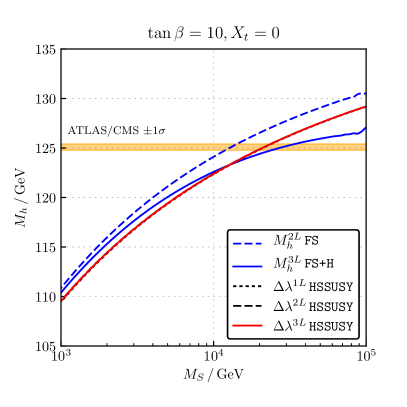
(a)

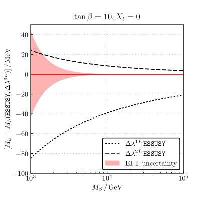
(b)

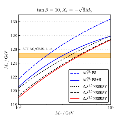
(c)

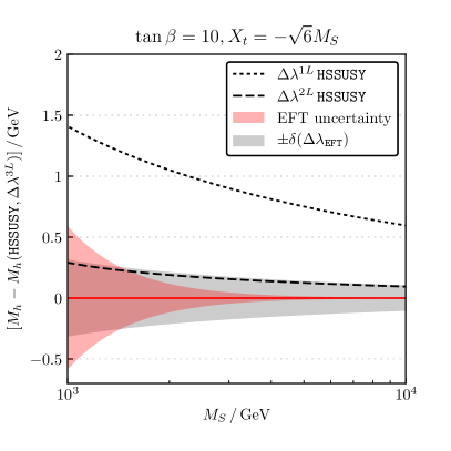
(d)

Figure 1: Comparison of the three-loop HSSUSY (EFT) calculation with lower order EFT and fixed-order MSSM calculations from the FlexibleSUSY package as a function of the SUSY scale. The orange band marks the experimentally measured value of the Higgs mass as written in Eq. (1).

In Fig. 1 the effect of $(\Delta\lambda_{\texttt{EFT}})_{\bar{\alpha}_{t}^{2}\bar{a}_{s}^{2}}$ on the pure EFT calculation of HSSUSY is shown as a function of the SUSY scale $M_{S}$ for degenerate soft-breaking mass parameters, all set equal to $M_{S}$. Furthermore, we set $\mu(\mu_{S})=m_{A}(\mu_{S})=\mu_{S}$, $\tan\beta(\mu_{S})=10$, $A_{t}=X_{t}+\mu/\tan\beta$, while all other trilinear couplings are set to zero. The upper row shows a scenario with vanishing stop mixing, $X_{t}(\mu_{S})=0$, the lower row shows one with maximal stop mixing, $X_{t}(\mu_{S})=-\sqrt{6}M_{S}$. The left column of Fig. 1 displays the value of the calculated Higgs boson mass for these two scenarios. The blue dashed line and the blue solid line show the two- and three-loop fixed-order calculations of FlexibleSUSY 2.1.0 and FlexibleSUSY 2.1.0+Himalaya 2.0.1, respectively. The black dotted, dashed, and red solid line depict the EFT calculations of HSSUSY with $\bar{\lambda}(\mu_{S})$ calculated at the one-, two-, and three-loop level, respectively. Here, $\Delta\lambda^{1L}$ and $\Delta\lambda^{2L}$ denote all available one- and two-loop corrections, respectively, and $\Delta\lambda^{3L}=(\Delta\lambda_{\texttt{EFT}})_{\bar{\alpha}_{t}^{2}\bar{a}_{s}^{2}}$. For comparison, the yellow horizontal band shows the current experimental value for the Higgs mass, see Eq. (1). As was already observed for example in Refs. [18, 17, 14], we find that in the range $M_{S}\geq 1\,\text{TeV}$ the fixed-order and the EFT calculations deviate by several GeV. This is to be expected, because the EFT calculation resums the large logarithmic corrections (in contrast to the fixed-order calculation) and above $M_{S}\gtrsim 1\,\text{TeV}$ the neglected terms of ${\cal O}(\bar{v}^{2}/M_{S}^{2})$ are negligible [13, 17, 19].

As the black dashed and solid red line are hardly distinguishable in these plots, we show the shift relative to the one- and two-loop calculations of HSSUSY in the right column of Fig. 1. The gray band in Fig. 1d corresponds to the theoretical uncertainty on the result due to the hierarchy expansions of the H3m result, evaluated according to Eq. (47); it amounts to more than 100% of the central shift for maximal mixing. For $X_{t}=0$, this uncertainty is zero, see Eq. (46), because we also set $\mu_{S}=M_{S}$. This is consistent with the fact that in this case, the degenerate-mass limit of the H3m result is exact. The red band shows the “EFT uncertainty” as defined in Refs. [10, 11, 14], estimating effects from missing terms of ${\cal O}(\bar{v}^{2}/M_{S}^{2})$. We see that the impact of $(\Delta\lambda_{\texttt{EFT}})_{\bar{\alpha}_{t}^{2}\bar{a}_{s}^{2}}$ is largely negative with respect to the two-loop threshold correction, $\Delta\lambda^{2L}$, and may reduce the Higgs mass by up to $0.6\,\text{GeV}$ for maximal mixing when considering all values in the grey uncertainty band. For zero stop mixing, the shift is significantly smaller ($\lesssim 20\,\text{MeV}$).

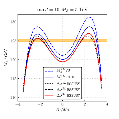
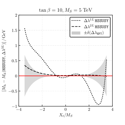
Figure 2: Comparison of the three-loop HSSUSY (EFT) calculation with lower order EFT and fixed-order MSSM calculations from the FlexibleSUSY package as a function of the relative stop mixing.

In Fig. 2, the Higgs mass prediction is shown as a function of the relative stop mixing parameter $x_{t}=X_{t}/M_{S}$ for a scenario with $\tan\beta=10$ and $M_{S}=5\,\text{TeV}$, where both the fixed-order and the EFT approach can accommodate for the experimentally observed value of $M_{h}$, Eq. (1), as long as $|x_{t}|$ is sufficiently large. The right panel shows again the difference of the three-loop calculation of HSSUSY with respect to the one- and two-loop calculations. In accordance with Fig. 1, we find that the shift induced by including $(\Delta\lambda_{\texttt{EFT}})_{\bar{\alpha}_{t}^{2}\bar{a}_{s}^{2}}$ is negative by trend, and below about $200\,\text{MeV}$ for $x_{t}>-2$. Below that value, the effects could be of order $1\,\text{GeV}$, but the uncertainty of our approximation grows to about 100% in this case, because the $x_{t}^{4}$ term is not included in the hierarchy expansion of the H3m result for this scenario.

To get an idea of the maximal effect that $(\Delta\lambda_{\texttt{EFT}})_{\bar{\alpha}_{t}^{2}\bar{a}_{s}^{2}}$ can have on the Higgs mass prediction, the blue band of Fig. 3 shows the variation of $M_{h}$ when the SUSY mass parameters $m_{Q,3}$, $m_{U,3}$, $m_{D,3}$, and $m_{\tilde{g}}$ are varied simultaneously and independently within the interval $[M_{S}/\sqrt{2},\sqrt{2}M_{S}]$ as a function of $M_{S}$, including the uncertainty $\delta((\Delta\lambda_{\texttt{EFT}})_{\bar{\alpha}_{t}^{2}\bar{a}_{s}^{2}})$. The hatched region marks the range of SUSY scales where the lightest running stop mass is below $1\,\text{TeV}$ for at least one of the scanned points; in this case, the EFT may not be applicable. For zero stop mixing (left panel), we find that $(\Delta\lambda_{\texttt{EFT}})_{\bar{\alpha}_{t}^{2}\bar{a}_{s}^{2}}$ can have an effect up to $\approx-150\,\text{MeV}$ for $M_{S}\geq 1\,\text{TeV}$. In the region where $m_{\tilde{t}_{1}}>1\,\text{TeV}$, the correction reduces to $-130\,\text{MeV}$ at most. The three-loop correction decreases for larger SUSY scales, mainly due to the fact that the SM couplings become smaller. For maximal stop mixing, $x_{t}=-\sqrt{6}$, the effect of the three-loop correction is significantly larger, and can reach $-1.25\,\text{GeV}$ for $m_{\tilde{t}_{1}}\gtrsim 1\,\text{TeV}$. The correction becomes particularly large when the soft-breaking stop-mass parameters $m_{Q,3}$ and $m_{U,3}$ become small.

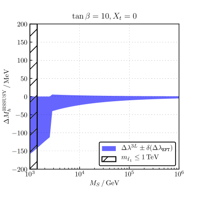
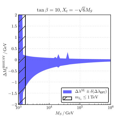
Figure 3: Variation of $M_{h}$ when the SUSY mass parameters are varied within the interval $[M_{S}/\sqrt{2},\sqrt{2}M_{S}]$ in HSSUSY for $\tan\beta=10$. The left panel shows $X_{t}=0$ and the right panel $X_{t}=-\sqrt{6}M_{S}$. The blue band shows the maximal variation of $M_{h}$ when the three-loop correction $(\Delta\lambda_{\texttt{EFT}})_{\bar{\alpha}_{t}^{2}\bar{a}_{s}^{2}}\pm\delta((\Delta\lambda_{\texttt{EFT}})_{\bar{\alpha}_{t}^{2}\bar{a}_{s}^{2}})$ is included, with respect to the two-loop calculation. In the hatched region there is $m_{\tilde{t}_{1}}(M_{S})\leq 1\,\text{TeV}$ for at least one of the scanned parameter points.

5 Conclusions

We have calculated the light CP-even Higgs mass of the MSSM by including all known fixed-order radiative corrections through ${\cal O}(\alpha_{t}^{2}\alpha_{s}^{2})$, and resumming the logarithmically enhanced terms for a heavy SUSY spectrum through fourth logarithmic order in SUSY QCD. The only ingredient entering this result that was unavailable in the literature up to now was the three-loop matching coefficient at ${\cal O}(\alpha_{t}^{2}\alpha_{s}^{2})$ for the quartic Higgs coupling from the SM to the MSSM. We derived it from the known three-loop corrections to the light CP-even Higgs boson mass of Refs. [34, 35]. The coefficient is provided both in terms of $\overline{\text{{DR}}}^{\prime}$ and $\overline{\text{{MS}}}$ parameters through its implementation into the public Himalaya library, version 2.0.1. This should facilitate its inclusion into spectrum generators which implement the EFT approach. An uncertainty estimate is provided to account for missing higher order terms in the mass hierarchy expansions.

Implementing $(\Delta\lambda)_{\alpha_{t}^{2}a_{s}^{2}}$ through Himalaya 2.0.1 into HSSUSY, our numerical analysis shows that the three-loop correction tends to be negative and may decrease the predicted Higgs boson pole mass by up to $0.6\,\text{GeV}$ for maximal stop mixing. In scenarios with zero stop mixing, the shift is significantly smaller, dropping to about $-25\,\text{MeV}$ for SUSY mass parameters of around $1\,\text{TeV}$. For non-degenerate spectra with $m_{\tilde{t}_{1}}\gtrsim 1\,\text{TeV}$, the three-loop correction can be of the same size and reach up to $-1.25\,\text{GeV}$ for low stop masses in scenarios where a suitable mass hierarchy exists. In scenarios where no such hierarchy exists the correction may be significantly larger, accompanied by a large expansion uncertainty.

Appendix A Documentation of Himalaya 2.0.1

In this section we summarize technical details concerning the new functionality of Himalaya 2.0.1.

Changes in Himalaya 2.0.1

In Himalaya 2.0.1, we made changes to the hierarchy selection and to some three-loop expressions which may affect the calculated Higgs mass at three-loop level. We list all of these changes below.

• In Himalaya 1.0.1, all input parameters are assumed to be given in the “H3m scheme”, see Sect. 3.2, and the output is provided in the same scheme by default. Since most MSSM spectrum generators use the $\overline{\text{{DR}}}^{\prime}$ scheme, we have changed the definition of the input and output accordingly: In Himalaya 2.0.1, all input parameters are assumed to be given in the $\overline{\text{{DR}}}^{\prime}$ scheme. The output is provided in the $\overline{\text{{DR}}}^{\prime}$ scheme by default. Shifts to other renormalization schemes (H3m, $\overline{\text{{MDR}}}^{\prime}$, …) are provided separately by Himalaya.

• There are parameter scenarios where none of the H3m hierarchies fits to the SUSY mass spectrum. H3m as well as Himalaya 1.0.1 used the h3 hierarchy in these cases, despite the fact that it does actually not fit. It turns out that the requirement

  $$m_{\tilde{t}_{2}} >1.3m_{\tilde{q}}\,, m_{\tilde{g}} >1.3m_{\tilde{q}}$$ (48)

  is sufficient to avoid these scenarios. Himalaya 2.0.1 will therefore throw an exception if the conditions (48) are not met.

• For the highest order in $(m_{\tilde{q}}^{2}-m_{\tilde{t}_{i}}^{2})$ in the hierarchy expansions of H3m, we found disagreement with the logarithmic terms of the EFT approach. We therefore discarded these orders completely (also the non-logarithmic terms) in Himalaya.

Input parameters.

With Himalaya 2.0.1 we extend the input parameters struct to a more general form. Its new form is summarized in the following listing:

⬇

typedef Eigen::Matrix<double,2,1> V2;

typedef Eigen::Matrix<double,3,3> RM33;

struct Parameters {

// DR’-bar parameters

double scale{}; // renormalization scale

double mu{}; // mu parameter, convention of

// [Phys.Rept. 117 (1985) 75-263]

double g1{}; // GUT-normalized gauge coupling g1, with

// gY = g1*Sqrt[3/5]

double g2{}; // gauge coupling g2 of SU(2)

double g3{}; // gauge coupling g3 of SU(3)

double vd{}; // VEV of down Higgs, with

// v = Sqrt[vu^2 + vd^2] ~ 246 GeV

double vu{}; // VEV of up Higgs, with

// v = Sqrt[vu^2 + vd^2] ~ 246 GeV

RM33 mq2{RM33::Zero()}; // soft-breaking squared left-handed

// squark mass parameters

RM33 md2{RM33::Zero()}; // soft-breaking squared right-handed

// down-squark mass parameters

RM33 mu2{RM33::Zero()}; // soft-breaking squared right-handed

// up-squark mass parameters

RM33 ml2{RM33::Zero()}; // soft-breaking squared left-handed

// slepton mass parameters

RM33 me2{RM33::Zero()}; // soft-breaking squared right-handed

// slepton mass parameters

RM33 Au{RM33::Zero()}; // trilinear up type squark-Higgs

// coupling matrix

RM33 Ad{RM33::Zero()}; // trilinear down type squark-Higgs

// coupling matrix

RM33 Ae{RM33::Zero()}; // trilinear electron type squark-Higgs

// coupling matrix

RM33 Yu{RM33::Zero()}; // up-type yukawa coupling matrix

RM33 Yd{RM33::Zero()}; // down-type yukawa coupling matrix

RM33 Ye{RM33::Zero()}; // electron-type yukawa coupling matrix

// DR’-bar masses

double M1{}; // bino

double M2{}; // wino

double MG{}; // gluino

double MW{NaN}; // W

double MZ{NaN}; // Z

double Mt{NaN}; // top-quark

double Mb{NaN}; // down-quark

double Mtau{NaN}; // tau lepton

double MA{}; // CP-odd Higgs

V2 MSt{NaN, NaN}; // stops

V2 MSb{NaN, NaN}; // sbottoms

// DR’-bar mixing angles

double s2t{NaN}; // sine of 2 times the stop mixing angle

double s2b{NaN}; // sine of 2 times the sbottom mixing angle

};

The parameters initialized to NaN are optional and will be calculated internally if not set to a finite value by the user. Note that all input parameters are interpreted as running MSSM parameters in the $\overline{\text{{DR}}}^{\prime}$ scheme at the renormalization scale scale.

Calling Himalaya at the C++ level.

Since the input parameters and the output of Himalaya 2.0.1 are always defined in the $\overline{\text{{DR}}}^{\prime}$ scheme, we have removed the $\overline{\text{{MDR}}}$ flag in the constructor of the HierarchyCalculator. The following source code listing shows an example call of Himalaya 2.0.1:

⬇

// create a new parameter point

himalaya::parameters point;

point.scale = 1000.; // GeV

point.mu = 1000.; // GeV

// fill remaining parameters ...

// create the calculator class

himalaya::HierarchyCalculator hc(point);

// calculate all three-loop corrections of O(at*as^2)

himalaya::HierarchyObject hoTop = hc.calculateDMh3L(false);

The HierarchyCalculator class takes the parameter point as the only mandatory argument. To calculate the three-loop corrections to the CP-even Higgs mass matrix or to the quartic Higgs coupling $\lambda$, one needs to call the calculateDMh3L member function of the created HierarchyCalculator object. The calculateDMh3L function takes a boolean argument to calculate the corrections of ${\cal O}(\alpha_{t}^{2}a_{s}^{2})$ (argument is false) or ${\cal O}(\alpha_{b}^{2}a_{s}^{2})$ (argument is true) to the CP-even Higgs mass matrix. The function returns a HierarchyObject which contains the calculated three-loop results.

To convert the three-loop results to other renormalization schemes, the HierarchyObject class provides new member functions which return additive shifts from the $\overline{\text{{DR}}}^{\prime}$ to any other scheme. The new member functions are listed in the following sub-section.

The following source code listing represents a complete example which illustrates how the three-loop correction of ${\cal O}(\alpha_{t}^{2}a_{s}^{2})$ to the CP-even Higgs mass matrix and to the quartic Higgs coupling can be calculated with Himalaya 2.0.1.

⬇

#include "HierarchyCalculator.hpp"

#include <cmath>

himalaya::Parameters make_point(double MS, double xt, double tb)

{

himalaya::Parameters pars;

const double MS2 = MS*MS;

const double Xt = xt*MS;

const double beta = std::atan(tb);

pars.scale = MS;

pars.mu = MS;

pars.g1 = 0.46;

pars.g2 = 0.65;

pars.g3 = 1.166;

pars.vd = 246*std::cos(beta);

pars.vu = 246*std::sin(beta);

pars.mq2 << MS2, 0, 0,

0, MS2, 0,

0, 0, MS2;

pars.md2 << MS2, 0, 0,

0, MS2, 0,

0, 0, MS2;

pars.mu2 << MS2, 0, 0,

0, MS2, 0,

0, 0, MS2;

pars.ml2 << MS2, 0, 0,

0, MS2, 0,

0, 0, MS2;

pars.me2 << MS2, 0, 0,

0, MS2, 0,

0, 0, MS2;

pars.Au(2,2) = Xt + pars.mu/tb;

pars.Yu(2,2) = 0.862;

pars.Yd(2,2) = 0.133;

pars.Ye(2,2) = 0.101;

pars.MA = MS;

pars.M1 = MS;

pars.M2 = MS;

pars.MG = MS;

return pars;

}

int main()

{

// create parameter point

const auto point = make_point(2000, std::sqrt(6.), 20);

// create calculator object

himalaya::HierarchyCalculator hc(point);

// calculate 3-loop corrections O(at^2*as^2)

const auto ho = hc.calculateDMh3L(false);

// get 3-loop contribution to CP-even Higgs mass matrix

const auto dMh_3L = ho.getDMh(3);

// get 3-loop contribution to lambda

const auto delta_lambda_3L = ho.getDLambda(3);

// get uncertainty for 3-loop lambda

const auto delta_lambda_3L_uncertainty = ho.getDLambdaUncertainty(3);

}

New member functions of HierarchyObject.

Below we list all member functions of HierarchyObject that are new in Himalaya 2.0.1.

getDMhDRbarPrimeToMDRbarPrimeShift()

Returns the additive shift to convert the Higgs mass matrix from the $\overline{\text{{DR}}}^{\prime}$ scheme at three-loop level to the $\overline{\text{{MDR}}}^{\prime}$ scheme.

getDMhDRbarPrimeToH3mShift()

Returns the additive shift to convert the Higgs mass matrix from the $\overline{\text{{DR}}}^{\prime}$ scheme at three-loop level to the H3m scheme. In matrix form, the shift is given by:

$$\begin{split}\left(\Delta M_{h,11}^{2}\right)_{\texttt{H3m}\to\overline{\text{{DR}}}^{\prime}}&=C\mu^{2}X_{t}^{2}\left\{m_{\tilde{t}_{1}}^{4}-2m_{\tilde{t}_{1}}^{2}m_{\tilde{t}_{2}}^{2}\ln\left(\frac{m_{\tilde{t}_{1}}^{2}}{m_{\tilde{t}_{2}}^{2}}\right)-m_{\tilde{t}_{2}}^{4}\right\},\end{split}$$ (49)

$$\begin{split}\left(\Delta M_{h,12}^{2}\right)_{\texttt{H3m}\to\overline{\text{{DR}}}^{\prime}}&=C\mu X_{t}\Bigg{\{}-m_{\tilde{t}_{1}}^{4}\left(A_{t}X_{t}+3m_{\tilde{t}_{2}}^{2}\right)+2A_{t}m_{\tilde{t}_{1}}^{2}m_{\tilde{t}_{2}}^{2}X_{t}\ln\left(\frac{m_{\tilde{t}_{1}}^{2}}{m_{\tilde{t}_{2}}^{2}}\right)\\ &\quad+A_{t}m_{\tilde{t}_{2}}^{4}X_{t}+m_{\tilde{t}_{1}}^{6}+3m_{\tilde{t}_{1}}^{2}m_{\tilde{t}_{2}}^{4}-m_{\tilde{t}_{2}}^{6}\Bigg{\}},\end{split}$$ (50)

$$\begin{split}\left(\Delta M_{h,21}^{2}\right)_{\texttt{H3m}\to\overline{\text{{DR}}}^{\prime}}&=\left(\Delta M_{h,12}^{2}\right)_{\texttt{H3m}\to\overline{\text{{DR}}}^{\prime}},\end{split}$$ (51)

$$\begin{split}\left(\Delta M_{h,22}^{2}\right)_{\texttt{H3m}\to\overline{\text{{DR}}}^{\prime}}&=C\Bigg{\{}\Delta_{12}\bigg{[}m_{\tilde{t}_{1}}^{2}\left(A_{t}^{2}X_{t}^{2}+4A_{t}m_{\tilde{t}_{2}}^{2}X_{t}-m_{\tilde{t}_{2}}^{4}\right)-m_{\tilde{t}_{1}}^{4}\left(2A_{t}X_{t}+m_{\tilde{t}_{2}}^{2}\right)\\ &\quad+\left(m_{\tilde{t}_{2}}^{3}-A_{t}m_{\tilde{t}_{2}}X_{t}\right)^{2}+m_{\tilde{t}_{1}}^{6}\bigg{]}-2A_{t}^{2}m_{\tilde{t}_{1}}^{2}m_{\tilde{t}_{2}}^{2}X_{t}^{2}\ln\left(\frac{m_{\tilde{t}_{1}}^{2}}{m_{\tilde{t}_{2}}^{2}}\right)\Bigg{\}},\end{split}$$ (52)

with

$$C=-\frac{8\alpha_{t}^{2}a_{s}^{2}v^{2}s_{\beta}^{2}}{m_{\tilde{t}_{1}}^{2}m_{\tilde{t}_{2}}^{2}\Delta_{12}^{3}}\Bigg{\{}-6(l_{S{\tilde{g}}}+1)m_{\tilde{g}}^{2}+10(l_{S{\tilde{q}}}+1)m_{\tilde{q}}^{2}+\sum_{i=1}^{2}(1+l_{S{{\tilde{t}}}_{i}})m_{\tilde{t}_{i}}^{2}\Bigg{\}}.$$ (53)

getDLambda(int loops)

Returns the correction to the matching relation of $\lambda$ at $n$-loop(s) including prefactors. $n$ can be $0,1,2,3$, where $n=3$ corresponds to $(\Delta\lambda_{\texttt{EFT}})_{\alpha_{t}^{2}a_{s}^{2}}$.

getDLambdaDRbarPrimeToMSbarShift(int loops)

Returns the additive shift $(\delta\lambda)_{\alpha_{t}^{2}a_{s}^{2}}$ of Eq. (34), which accounts for the effect of a parameter conversion in $\lambda$ at $n$-loop(s) from the $\overline{\text{{DR}}}^{\prime}$ to the $\overline{\text{{MS}}}$ scheme, including prefactors. $n$ can be $0,1,2,3$, where $n=3$ corresponds to the shift for $(\Delta\lambda_{\texttt{EFT}})_{\alpha_{t}^{2}a_{s}^{2}}$.

getDLambdaUncertainty(int loops)

For $\texttt{loops}=3$ the function returns the uncertainty $\delta((\Delta\lambda_{\texttt{EFT}})_{\alpha_{t}^{2}a_{s}^{2}})$ according to Eq. (47), including the prefactors. For $\texttt{loops}\neq 3$ the function returns zero.

getDMh2EFT(int loops)

Returns $M_{h,\text{{EFT}},\texttt{<loops>}}^{2}$ according to Eq. (23) at $n$-loop(s). $n$ can be $0$, $1$, $2$, $3$, where $n=3$ includes the contribution of $(\Delta\lambda_{\texttt{EFT}})_{\alpha_{t}^{2}a_{s}^{2}}$. The three-loop result getDMh2EFT(3) can be used to extract $(\Delta\lambda)_{\alpha_{t}^{2}a_{s}^{2}}$ from an alternative fixed-order calculation, following the procedure introduced in this paper. See below for an example.

Extracting $(\Delta\lambda)_{\alpha_{t}^{2}a_{s}^{2}}$ from alternative three-loop calculations of the Higgs mass.

The results for matching coefficient $(\Delta\lambda_{\texttt{EFT}})_{\alpha_{t}^{2}a_{s}^{2}}$ presented in this paper rely on the H3m result for the three-loop Higgs mass. By using the member functions getDMh2EFT(int) and getDLambda(int) of the HierarchyObject, it is possible to extract the three-loop correction $(\Delta\lambda)_{\alpha_{t}^{2}a_{s}^{2}}$ from any other three-loop fixed-order $\overline{\text{{DR}}}^{\prime}$ ${\cal O}(\alpha_{t}^{2}a_{s}^{2})$ expression for the Higgs mass. These two member functions return the following three-loop contributions

getDMh2EFT(3) $$=M_{h,\text{{EFT}},3}^{2}\bigg{|}_{(\Delta\lambda)_{\alpha_{t}^{2}a_{s}^{2}}=0}+\kappa^{3}v^{2}\alpha_{t}^{2}a_{s}^{2}s_{\beta}^{4}(\Delta\lambda_{\texttt{EFT}})_{\alpha_{t}^{2}a_{s}^{2}}-M_{h,\text{{EFT}},2}^{2}\,,$$ (54)

getDLambda(3) $$=\kappa^{3}\alpha_{t}^{2}a_{s}^{2}s_{\beta}^{4}(\Delta\lambda_{\texttt{EFT}})_{\alpha_{t}^{2}a_{s}^{2}}\,.$$ (55)

with $M_{h,\text{{EFT}},n}^{2}$ and $(\Delta\lambda_{\texttt{EFT}})_{\alpha_{t}^{2}a_{s}^{2}}$ defined in Sect. 3. By combining these functions with an alternative three-loop calculation $M^{2}_{h,\text{{EFT}},3}$ as

$$(\Delta\lambda_{\text{alt}})_{\alpha_{t}^{2}a_{s}^{2}}\,v^{2} =M_{h,\text{{EFT}},3}^{2}-M_{h,\text{{EFT}},2}^{2}-\texttt{getDMh2EFT(3)}+v^{2}\times\texttt{getDLambda(3)}$$ (56)

$$=M^{2}_{h,\text{{EFT}},3}-M_{h,\text{{EFT}},3}^{2}(\mu_{t},\mu_{S})\bigg{|}_{(\Delta\lambda)_{\alpha_{t}^{2}a_{s}^{2}}=0}$$ (57)

one can extract the corresponding three-loop correction $(\Delta\lambda_{\text{alt}})_{\alpha_{t}^{2}a_{s}^{2}}$.

References

- [1] G. Aad et al. [ATLAS and CMS Collaborations], Phys. Rev. Lett. 114 (2015) 191803 [arXiv:1503.07589 [hep-ex]].
- [2] H.E. Haber and R. Hempfling, Phys. Rev. Lett. 66 (1991) 1815.
- [3] Y. Okada, M. Yamaguchi and T. Yanagida, Prog. Theor. Phys. 85 (1991) 1.
- [4] J.R. Ellis, G. Ridolfi and F. Zwirner, Phys. Lett. B 257 (1991) 83.
- [5] J.R. Ellis, G. Ridolfi and F. Zwirner, Phys. Lett. B 262 (1991) 477.
- [6] R. Barbieri and M. Frigeni, Phys. Lett. B 258 (1991) 395.
- [7] P.H. Chankowski, S. Pokorski and J. Rosiek, Nucl. Phys. B 423 (1994) 437 [hep-ph/9303309].
- [8] A. Dabelstein, Z. Phys. C 67 (1995) 495 [hep-ph/9409375].
- [9] B.C. Allanach, A. Djouadi, J.L. Kneur, W. Porod and P. Slavich, JHEP 0409 (2004) 044 [hep-ph/0406166].
- [10] E. Bagnaschi, G.F. Giudice, P. Slavich and A. Strumia, JHEP 1409 (2014) 092 [arXiv:1407.4081 [hep-ph]].
- [11] J. Pardo Vega and G. Villadoro, JHEP 1507 (2015) 159 [arXiv:1504.05200 [hep-ph]].
- [12] H. Bahl and W. Hollik, Eur. Phys. J. C 76 (2016) no.9, 499 [arXiv:1608.01880 [hep-ph]].
- [13] H. Bahl, S. Heinemeyer, W. Hollik and G. Weiglein, Eur. Phys. J. C 78 (2018) no.1, 57 [arXiv:1706.00346 [hep-ph]].
- [14] B.C. Allanach and A. Voigt, Eur. Phys. J. C 78 (2018) no.7, 573 [arXiv:1804.09410 [hep-ph]].
- [15] E. Bagnaschi, J. Pardo Vega and P. Slavich, Eur. Phys. J. C 77 (2017) no.5, 334 [arXiv:1703.08166 [hep-ph]].
- [16] T. Hahn, S. Heinemeyer, W. Hollik, H. Rzehak and G. Weiglein, Phys. Rev. Lett. 112 (2014) no.14, 141801 [arXiv:1312.4937 [hep-ph]].
- [17] P. Athron, M. Bach, D. Harries, T. Kwasnitza, J.h. Park, D. Stöckinger, A. Voigt and J. Ziebell, Comput. Phys. Commun. 230 (2018) 145 [arXiv:1710.03760 [hep-ph]].
- [18] P. Athron, J. h. Park, T. Steudtner, D. Stöckinger and A. Voigt, JHEP 1701 (2017) 079 [arXiv:1609.00371 [hep-ph]].
- [19] F. Staub and W. Porod, Eur. Phys. J. C 77 (2017) no.5, 338 [arXiv:1703.03267 [hep-ph]].
- [20] H. Bahl and W. Hollik, JHEP 1807 (2018) 182 [arXiv:1805.00867 [hep-ph]].
- [21] P. Athron, J. h. Park, D. Stöckinger and A. Voigt, Comput. Phys. Commun. 190 (2015) 139 [arXiv:1406.2319 [hep-ph]].
- [22] W. Porod, Comput. Phys. Commun. 153 (2003) 275 [hep-ph/0301101].
- [23] F. Staub, Comput. Phys. Commun. 181 (2010) 1077 [arXiv:0909.2863 [hep-ph]].
- [24] W. Porod and F. Staub, Comput. Phys. Commun. 183 (2012) 2458 [arXiv:1104.1573 [hep-ph]].
- [25] F. Staub, Comput. Phys. Commun. 182 (2011) 808 [arXiv:1002.0840 [hep-ph]].
- [26] F. Staub, Comput. Phys. Commun. 184 (2013) 1792 [arXiv:1207.0906 [hep-ph]].
- [27] F. Staub, Comput. Phys. Commun. 185 (2014) 1773 [arXiv:1309.7223 [hep-ph]].
- [28] B.C. Allanach, Comput. Phys. Commun. 143 (2002) 305 [hep-ph/0104145].
- [29] B.C. Allanach, A. Bednyakov and R. Ruiz de Austri, Comput. Phys. Commun. 189 (2015) 192 [arXiv:1407.6130 [hep-ph]].
- [30] A. Djouadi, J.L. Kneur and G. Moultaka, Comput. Phys. Commun. 176 (2007) 426 [hep-ph/0211331].
- [31] S.P. Martin, Phys. Rev. D 92 (2015) no.5, 054029 [arXiv:1508.00912 [hep-ph]].
- [32] K.G. Chetyrkin and M.F. Zoller, JHEP 1606 (2016) 175 [arXiv:1604.00853 [hep-ph]].
- [33] P. Draper, G. Lee and C.E.M. Wagner, Phys. Rev. D 89 (2014) no.5, 055023 [arXiv:1312.5743 [hep-ph]].
- [34] R.V. Harlander, P. Kant, L. Mihaila and M. Steinhauser, Phys. Rev. Lett. 100 (2008) 191602 [Phys. Rev. Lett. 101 (2008) 039901] [arXiv:0803.0672 [hep-ph]].
- [35] P. Kant, R.V. Harlander, L. Mihaila and M. Steinhauser, JHEP 1008 (2010) 104 [arXiv:1005.5709 [hep-ph]].
- [36] R.V. Harlander, J. Klappert and A. Voigt, Eur. Phys. J. C 77 (2017) no.12, 814 [arXiv:1708.05720 [hep-ph]].
- [37] I. Jack, D.R.T. Jones, S.P. Martin, M.T. Vaughn and Y. Yamada, Phys. Rev. D 50 (1994) R5481 [hep-ph/9407291].
- [38] S.P. Martin, Phys. Rev. D 75 (2007) 055005 [hep-ph/0701051].
- [39] S.P. Martin and D.G. Robertson, Phys. Rev. D 90 (2014) no.7, 073010 [arXiv:1407.4336 [hep-ph]].
- [40] G. Degrassi, P. Slavich and F. Zwirner, Nucl. Phys. B 611 (2001) 403 [hep-ph/0105096].
- [41] S.P. Martin, Phys. Rev. D 65 (2002) 116003 [hep-ph/0111209].
- [42] S.P. Martin, Phys. Rev. D 66 (2002) 096001 [hep-ph/0206136].
- [43] S.P. Martin, Phys. Rev. D 67 (2003) 095012 [hep-ph/0211366].
- [44] D.M. Capper, D.R.T. Jones and P. van Nieuwenhuizen, Nucl. Phys. B 167 (1980) 479.
- [45] D. Stöckinger JHEP 0503 (2005) 076 [hep-ph/0503129].
- [46] D. Stöckinger and J. Unger, Nucl. Phys. B 935 (2018) 1 [arXiv:1804.05619 [hep-ph]].
- [47] R.V. Harlander, L. Mihaila and M. Steinhauser, Eur. Phys. J. C 63 (2009) 383 [arXiv:0905.4807 [hep-ph]].
- [48] R.V. Harlander, D.R.T. Jones, P. Kant, L. Mihaila and M. Steinhauser, JHEP 0612 (2006) 024 [hep-ph/0610206].
- [49] W. Siegel, Phys. Lett. B 84 (1979) 193.
- [50] A. Bednyakov, A. Onishchenko, V. Velizhanin and O. Veretin, Eur. Phys. J. C 29 (2003) 87 [hep-ph/0210258].
- [51] A. Bednyakov, D.I. Kazakov and A. Sheplyakov, Phys. Atom. Nucl. 71 (2008) 343 [hep-ph/0507139].
- [52] S.P. Martin and M. T. Vaughn, Phys. Lett. B 318 (1993) 331 [hep-ph/9308222].
- [53] B. Summ and A. Voigt, JHEP 1808 (2018) 026 [arXiv:1806.05171 [hep-ph]].
- [54] https://www.ttp.kit.edu/Progdata/ttp10/ttp10-23/
- [55] T. Hermann, L. Mihaila and M. Steinhauser, Phys. Lett. B 703 (2011) 51 [arXiv:1106.1060 [hep-ph]].
- [56] Wolfram Research, Inc., Mathematica, Version 11.3, Champaign, IL (2018).
- [57] A.V. Bednyakov, A.F. Pikelner and V.N. Velizhanin, Phys. Lett. B 722 (2013) 336 [arXiv:1212.6829 [hep-ph]].
- [58] A.V. Bednyakov, A.F. Pikelner and V.N. Velizhanin, Nucl. Phys. B 875 (2013) 552 [arXiv:1303.4364 [hep-ph]].
- [59] L.N. Mihaila, J. Salomon and M. Steinhauser, Phys. Rev. D 86 (2012) 096008 [arXiv:1208.3357 [hep-ph]].
- [60] D. Buttazzo, G. Degrassi, P.P. Giardino, G.F. Giudice, F. Sala, A. Salvio and A. Strumia, JHEP 1312 (2013) 089 [arXiv:1307.3536 [hep-ph]].
- [61] A.V. Bednyakov and A.F. Pikelner, Phys. Lett. B 762 (2016) 151 [arXiv:1508.02680 [hep-ph]].
- [62] S. Fanchiotti, B.A. Kniehl and A. Sirlin, Phys. Rev. D 48 (1993) 307 [hep-ph/9212285].
- [63] K.G. Chetyrkin and M. Steinhauser, Nucl. Phys. B 573 (2000) 617 [hep-ph/9911434].
- [64] K. Melnikov and T. van Ritbergen, Phys. Lett. B 482 (2000) 99 [hep-ph/9912391].
- [65] K.G. Chetyrkin, J.H. Kühn and M. Steinhauser, Comput. Phys. Commun. 133 (2000) 43 [hep-ph/0004189].
- [66] G. Degrassi, S. Di Vita, J. Elias-Miro, J.R. Espinosa, G.F. Giudice, G. Isidori and A. Strumia, JHEP 1208 (2012) 098 [arXiv:1205.6497 [hep-ph]].