Paired Comparison Sentiment Scores

Abstract

The method of paired comparisons is an established method in psychology. In this article, it is applied to obtain continuous sentiment scores for words from comparisons made by test persons. We created an initial lexicon with $n=199$ German words from a two-fold all-pair comparison experiment with ten different test persons. From the probabilistic models taken into account, the logistic model showed the best agreement with the results of the comparison experiment. The initial lexicon can then be used in different ways. One is to create special purpose sentiment lexica through the addition of arbitrary words that are compared with some of the initial words by test persons. A cross-validation experiment suggests that only about 18 two-fold comparisons are necessary to estimate the score of a new, yet unknown word, provided these words are selected by a modification of a method by Silverstein & Farrell. Another application of the initial lexicon is the evaluation of automatically created corpus-based lexica. By such an evaluation, we compared the corpus-based lexica SentiWS, SenticNet, and SentiWordNet, of which SenticNet 4 performed best. This technical report is a corrected and extended version of a presentation made at the ICDM Sentire workshop in 2016.

1 Introduction

A sentiment lexicon is a dictionary that assigns each term a polarity score representing the strength of the positive or negative affect associated with the term. In general, word polarity strength depends on the context, and its representation by a single number can therefore only be a crude approximation. Nevertheless, such sentiment lexica are an important tool for opinion mining and have been proven to be very useful. Examples for recent use cases are the sentiment analysis of tweets and SMS [1, 2] or the political classification of newspapers [3].

There are two approaches to building a sentiment lexicon: corpus based automatic assignment or manual annotation. Corpus based approaches start with a set of seed words of known polarity and extend this set with other words occurring in a text corpus or a synonym lexicon. One possible approach is to compute the “Pointwise Mutual Information” (PMI) [4] from co-occurrences of seed words and other words. The German sentiment lexicon SentiWS [5] was built in this way. The English sentiment lexicon SentiWordNet [6] is based on the propagation of seed words, too, but by means of semi-supervised classification and random walks. Yet another sophisticated corpus-based method was implemented by Cambria et al. for SenticNet [7, 8, 9].

Corpus based methods have the advantage of building large lexica in an automated way without time consuming experiments with human annotators. They have two drawbacks, however: due to peculiarities in the corpus, some words can obtain strange scores. In SentiWS 1.8, e.g., “gelungen” (successful) has the highest positive score (1.0) while the more positive word “fantastisch” (fantastic) only has a score of 0.332. In SenticNet 3.0, “inconsequent” has a strong positive polarity (0.948). Moreover, it is not possible to assign a score value to words that are absent from the corpus.

Assigning polarity scores by manual annotations can be done in two different ways. One is by direct assignment of an ordinal score to each word on a Likert-type scale. In this way, Wilson et al. have created a subjectivity lexicon with English words [10], which has also been used by means of automated translations for sentiment analysis of German texts [11]. The other method is to present words in pairs and let the observer decide which word is more positive or more negative. Comparative studies for other use cases have shown that scores from paired comparisons are more accurate than direct assignments of scores [12]. The main advantage is their invariance to scale variances between different test persons. This is especially important when words are added at some later point when the original test persons are no longer available. Unfortunately, paired comparisons are much more expensive than direct assignments: for $n$ words, direct assignments only require $O(n)$ judgments, while a complete comparison of all pairs requires $O(n^{2})$ judgments. For large $n$, this becomes prohibitive and must be replaced by incomplete comparisons, i.e. by omitting pairs. Incomplete paired comparisons are widely deployed in the estimation of chess players’ strength [13, 14].

In the present article, we propose a method for building a sentiment lexicon from paired comparisons in two steps. At first, an initial lexicon is built from a limited set of 199 words by comparison of all pairs. This lexicon is then subsequently extended with new words, which are only compared to a limited number of words from the initial set, which are determined by a modified version of Silverstein & Farrell’s sorting method [15].

As we plan to use the lexicon ourselves for the sentiment analysis of German news reporting and thus were in need of a reliable German sentiment lexicon, and as our test persons were native German speakers, the scope of our investigation was restricted to German words. In order to use this lexicon for an evaluation of English lexica, we utilized the “averaged translation” technique described in Sec. 4.4. Automatic translation is a common method in multilingual sentiment analysis [16, 17]. It should be noted, however, that the ground truth scores of our new sentiment lexicon can only be used to compare sentiment lexica with respect to their accuracy in the sentiment analysis of German texts.

This article is an extended and corrected version of a presentation made at the ICDM workshop “Sentire” in December 2016 [18]. Compared to that presentation, the following changes and additions have been made:

1. The scores in [18] had been computed with an approximation by Elo that turned out to be grossly inaccurate in this use case [19]. The formula has been replaced by a numeric optimization and all scores have been recomputed. This correction also fixes the odd result of the leave-one-out experiment in [18].

2. The validity of the probabilistic model is checked and validated with a $\chi^{2}$ goodness-of-fit test.

3. The two large English sentiment lexica SenticNet 4.0 [9] and SentiWordNet 3.0 [6] have been included in the evaluation by means of averaged translation.

4. An error inherited from SentiWS has been corrected that had lead to a duplicate word in two different spellings, which has been corrected by merging the duplicates.

Our article is organized as follows: Sec. 2 provides an overview over the mathematical model that underpins the method of paired comparisons and presents formulas for computing scores from paired comparison results, Sec. 3 describes the criteria for choosing the initial set of words and our experimental setup, and Sec. 4 presents the results for the initial lexicon, evaluates the method for adding new words, and presents an evaluation of the other lexica Sentiws, SenticNet, and SentiWordNet by means of our ground truth initial lexicon.

2 Method of paired comparison

The method of paired comparison goes back to the early 20th century [20]. See [14] for a comprehensive presentation of the model and its estimation problems, and [21] for a review of recent extensions. Applied to word polarity, it makes the assumption that each word $w_{i}$ has a hidden score (or rating) $r_{i}$. The probability that $w_{i}$ is more positive than $w_{j}$ (symbolically: $w_{i}>w_{j}$) in a randomly chosen context depends on the difference between the hidden scores:

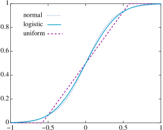
Figure 1: Different choices for the cumulative distribution function $F$ with identical standard deviations $\sigma=1/3$.

$$P(w_{i}>w_{j}) =F(r_{i}-r_{j}-t)$$ (1a)

$$P(w_{i}\approx w_{j}) =F(r_{i}-r_{j}+t)-F(r_{i}-r_{j}-t)$$ (1b)

$$P(w_{i}<w_{j}) =F(r_{j}-r_{i}-t)$$ (1c)

where $t$ is approximately proportional to the drawing probability of equal strength players and can thus be considered as a draw width, and $F$ is the cumulative distribution function of a zero-symmetric random variable. Thurstone’s model [20] uses an $F$ based on the normal distribution, a model that can be derived from the assumption that the polarity of a word $w_{i}$ is normally distributed around its mean inherent score $r_{i}$. Although this is the only model with a sound statistical justification, simpler distribution functions have also been used for convenience, e.g. the logistic distribution (Bradley-Terry model) [22] or the uniform distribution [23]. The shapes of these functions are quite similar (see Fig. 1), and they typically provide similar fits to data [24], although the asymptotic error of the score estimates behaves differently [25]. The standard deviation $\sigma$ of the distribution function $F$ is a scale parameter that determines the range of the ratings $r_{i}$. We have set it to $\sigma=1/3$ so that the estimated scores approximately fell into the range $[-1,1]$ for our data.

As the probabilities in Eq. (1) only depend on rating differences, the origin $r=0$ cannot be determined from the model, but must be defined by an external constraint. Typical choices are the average rating constraint $\sum_{i}r_{i}=0$, or the reference object constraint, i.e. $r_{i}=0$ for some $i$. For sentiment lexica, a natural constraint can be obtained by separately classifying words into positive and negative words and choosing the origin in such a way that the scores from the paired comparison model coincide with these classifications.

The ratings $r_{i}$ and the draw-width $t$ must be estimated from the observed comparisons. During our two steps of building a sentiment lexicon, two different estimation problems occur:

1. Estimation of one unknown $r$ of a new word from $m$ comparisons with old words with known ratings $q_{i},\ldots,q_{m}$.

2. Estimation of $t$ and all unknown $r_{1}\ldots,r_{n}$ from arbitrary pair comparisons.

In [18], analytic formulas were given for the estimators, but these were based on an approximation by Elo [13, paragraph 1.66] which turned out to be grossly inaccurate in this use case [19]. The formulas given in [18] should therefore not be used, and it is necessary instead to estimate the parameters via numeric optimization either with the maximum likelihood principle or with non-linear least squares.

2.1 Case 1: one unknown rating $r$

Let us first consider this simpler case. The log-likelihood function $\ell(r)$ ($t$ is considered as given) is

$$\ell(r) =\sum_{\mbox{\scriptsize\it wins}}\log F(r-q_{i}-t)$$ (2)

$$+\sum_{\mbox{\scriptsize\it draws}}\log\Big{(}F(r-q_{i}+t)-F(r-q_{i}-t)\Big{)}$$

$$+\sum_{\mbox{\scriptsize\it losses}}\log F(q_{i}-r-t)$$

As this is a function of only one variable $r$, it can be easily maximized numerically, e.g., with the R function optimize.

Batchelder & Bershed [14] suggested an alternative method-of-moments estimation by setting a combination of the observed number of wins $W$ and draws $D$ equal to its expectation value and solve the resulting equation for the parameters:

$$W+ D/2=\sum_{i=1}^{m}F(r-q_{i}-t)$$ (3)

$$+\frac{1}{2}\sum_{i=1}^{m}\Big{(}F(r-q_{i}+t)-F(r-q_{i}-t)\Big{)}$$

This combination is constructed in such a way that a Taylor expansion of the right hand side around $t=0$ cancels out the term linear in $t$, so that we obtain for small $t$

$$W+D/2=\sum_{i=1}^{m}F(r-q_{i})+O(t^{2})$$ (4)

Even this approximation must be solved numerically for $r$, but it makes the score estimation independent of the estimate for $t$, and it shows that the draw width has only little effect on the score estimator.

It should be noted that both the solution of (3) or (4) and the maximization of (2) yield $r=\infty$ (or $-\infty$) when $F$ is chosen to be the normal or logistic distribution and the word wins (or looses) all comparisons. For the uniform distribution, the solution or minimum is not unique in this case, but this ambiguity could be resolved by choosing the solution with $\min(|r|)$.

2.2 Case 2: all ratings $(r_{i})_{i=1}^{n}$ and $t$ unknown

The log-likelihood function in this case is

$$\ell( r_{1},\ldots,r_{n},t)=\sum_{\begin{subarray}{c}\mbox{\scriptsize\it comparisons}\\ {\mbox{\scriptsize\it with }w_{i}>w_{j}}\end{subarray}}\!\!\log F(r_{i}-r_{j}-t)$$ (5)

$$+\sum_{\begin{subarray}{c}\mbox{\scriptsize\it comparisons}\\ {\mbox{\scriptsize\it with }w_{i}\approx w_{j}}\end{subarray}}\!\!\log\Big{(}F(r_{i}-r_{j}+t)-F(r_{i}-r_{j}-t)\Big{)}$$

Due to the large number of $n+1$ parameters, numerical methods for maximizing the log-likelihood function (5) might be very slow or fail to converge. In this situation, an alternative solution obtained via the least-squares method can be helpful.

For a least squares fit of the parameters, let us consider the same observable as in case 1, but now for each word $w_{i}$:

$$S_{i}=\underbrace{W_{i}}_{\mbox{\scriptsize wins of word $w_{i}$}}+\quad\frac{1}{2}\underbrace{D_{i}}_{\mbox{\scriptsize draws of word $w_{i}$}}$$ (6)

When we set this “scoring” equal to its expectation value and make again a Taylor series expansion at $t=0$, we obtain

$$S_{i}=\sum_{j\in C_{i}}F(r_{i}-r_{j})+O(t^{2})$$ (7)

where $C_{i}$ are the indices of all words $w_{j}$ that have been compared with $w_{i}$. Joint estimates for all ratings can then be obtained by minimizing the sum of the squared deviations

$$SS(r_{1},\ldots,r_{n})=\sum_{i=1}^{n}\Big{(}S_{i}-\sum_{j\in C_{i}}F(r_{i}-r_{j})\Big{)}^{2}$$ (8)

Minimizing (8) is a non-linear least squares problem, which can be solved efficiently with the Levenberg-Marquardt algorithm as it is provided, e.g., by the R package minpack.lm [26].

To obtain an approximate estimator for the draw width $t$, let us consider the total number of draws $D_{i}$ of each word $w_{i}$ as an observable and set it equal to its expectation value from its $k_{i}$ comparisons:

$$D_{i}=\sum_{j\in C_{i}}\Big{(}F(r_{i}-r_{j}+t)-F(r_{i}-r_{j}-t)\Big{)}$$ (9)

Keeping only the first non-zero term in a Taylor expansion around $t=0$ of the sum on the right hand side yields

$$\sum_{j\in C_{i}}\Big{(}F(r_{i} -r_{j}+t)-F(r_{i}-r_{j}-t)\Big{)}$$

$$\approx\quad 2t\sum_{j\in C_{i}}F^{\prime}(r_{i}-r_{j})$$ (10)

Again, we can determine $t$ by minimizing the sum of the squared deviations

$$SS(t)=\sum_{i=1}^{n}\left(D_{i}-2t\sum_{j\in C_{i}}F^{\prime}(r_{i}-r_{j})\right)^{2}$$ (11)

The minimum of expression (11) can be found analytically by solving for the zero of $SS^{\prime}(t)$, which yields

$$t=\frac{\sum_{i=1}^{k_{i}}f_{i}D_{i}/2}{\sum_{i=1}^{k_{i}}f_{i}^{2}}\quad\mbox{ with}\quad f_{i}=\sum_{j\in C_{i}}F^{\prime}(r_{i}-r_{j})$$ (12)

The least-squares solution (8) and (12) can either be used as an estimator for the parameters, or it can be used as a starting point for maximizing the log-likelihood function.

3 Experimental design

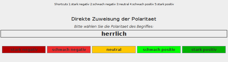
(a) direct assignment

(b) paired comparison

Figure 2: Graphical user interface for score assignment as seen by the test persons.

To select 200 words for building the initial lexicon from round robin pair comparisons, we have started with all $\numprint{1498}$ adjectives from SentiWS [5]. We have chosen adjectives because sentiments are more often carried by adjectives and adverbs than by verbs and nouns [27]. To build an intersection of these words with SenticNet [7], we translated all words into English with both of the German-English dictionaries from www.dict.cc and www.freedict.org, and removed all words without a match in SenticNet. From the remaining $\numprint{1303}$ words, we selected manually 10 words that appeared strongly positive to us, and 10 strongly negative words. This was to make sure that the polarity range is sufficiently wide in the initial lexicon. The remaining words were ranked by their SentiWS score and selected with equidistant ranks, such that we obtained 200 words, with an equal number of positive and negative words according to SentiWS. As we noticed after finishing the experiments, there are duplicate words in different spellings in SentiWS, and we eventually only had 199 different words by an unhappy coincidence. In the computations of section 4 in the present paper, we have taken care of this by correcting one of the spellings, i.e. replaced the word “phantastisch” with “fantastisch” (fantastic).

We let ten different test persons assign polarity scores to these words in two different experiments. The first one consisted of direct assignment of scores on a five degree scale (see Fig. 2(a)), which resulted in ten evaluations for each word. An average score was computed for each word by replacing the ordinal scale with a metric value ($-1$ = strong negative, $-0.5$ = weak negative, $0$ = neutral, $0.5$ = weak positive, $1.0$ = strong positive).

The second experiment consisted of twofold round robin paired comparisons between the original 200 words, with all $2\cdot\numprint{19900}$ pairs evenly distributed among the ten test persons, such that each person evaluated $\numprint{3980}$ pairs. Due to the duplicate word, this actually was not a round robin experiment, but one word (“fantastisch”) was compared more often than the others. See Fig. 2(b) for the graphical user interface presented to the test persons.

The scores were computed both with the maximum likelihood (ML) method and the non-linear least squares (LSQ) method as described in section 2.2. The standard deviation of the distribution function $F$ was set to $\sigma=1/3$, which corresponds to the distribution functions in Fig. 1. Maximization of the log-likelihood function (5) took about 12 minutes on an i7-4770 3.40 GHz with the “BFGS” method of the R-function optim. As this method uses numerically computed gradients, it was not applicable in the case of the uniform distribution, because its distribution function is not differentiable. We therefore resorted to the much slower optimization by Nelder & Mead in this case with the Elo approximate solution [18] as a starting point, which took 45 minutes. The LSQ solution, on the contrary, only took 12 seconds in all cases because we could use the more efficient Levenberg-Marquardt algorithm from the R package minpack.lm [26] for minimizing (8). When the LSQ solution was used as a starting point for the ML optimization, the runtime of the BFGS algorithm reduced to 6 minutes. This was not applicable in the case of the uniform distribution, though, because the LSQ solution corresponds to a log-likelihood function that is minus infinity.

For a reasonable choice for the origin $r=0$, we shifted all scores such that they best fitted to the discrimination between positive and negative words from the direct comparison experiment. To be precise: when $r^{\prime}_{i}$ is the score from the direct assignment and $r_{i}$ the score from the paired comparisons with an arbitrarily set origin, we chose the shift value $\rho$ that minimized the squared error

$$SE(\rho)\quad=\sum_{\operatorname{sign}(\rho+r_{i})\neq\operatorname{sign}(r^{\prime}_{i})}(\rho+r_{i})^{2}$$ (13)

Algorithm 1 One-fold addition of new word

1:word $w$ with unknown rating $r$, number of comparisons $m$, words $\vec{v}=(v_{1},\ldots,v_{n})$ sorted by their known ratings $q_{1},\ldots,q_{n}$

2:new rating $r$

3:$i_{l}\leftarrow 1$ and $i_{r}\leftarrow n$

4:$i\leftarrow\lfloor(i_{l}+i_{r})/2\rfloor$ $\triangleright$ might be randomized

5:$\vec{u}\leftarrow\vec{v}$ and $m_{0}\leftarrow 0$

6:$\vec{q}\leftarrow()$ and $\vec{S}\leftarrow()$

7:while $i>i_{l}$ and $i<i_{r}$ do $\triangleright$ binary search

8:   $m_{0}\leftarrow m_{0}+1$

9:   $\vec{q}\leftarrow\vec{q}\cup q_{i}$

10:   $s\leftarrow$ score from $w$ versus $v_{i}$ comparison,

11:         where win counts 1 and draw counts 1/2

12:   $\vec{S}\leftarrow\vec{S}\cup s$

13:   $\vec{u}\leftarrow\vec{u}\setminus v_{i}$

14:   if $s>1/2$ then

15:      $i_{l}\leftarrow i$

16:   else

17:      $i_{r}\leftarrow i$

18:   end if

19:   $i\leftarrow\lfloor(i_{l}+i_{r})/2\rfloor$ $\triangleright$ might be randomized

20:end while

21:$r_{0}\leftarrow(q_{i_{l}}+q_{i_{r}})/2$ $\triangleright$ first guess

22:$\vec{u}\leftarrow m-m_{0}$ words in $\vec{u}$ with closest ratings to $r_{0}$

23:$\vec{q}\leftarrow\vec{q}$ $\cup$ ratings of $\vec{u}$

24:$\vec{S}\leftarrow\vec{S}$ $\cup$ scores of $w$ against words from $\vec{u}$

25:$r\leftarrow$ LSQ estimate from $(\vec{S},\vec{q})$ $\triangleright$ cf. Sec. (2.1)

26:return $r$

For adding new words, we implemented the method by Silverstein & Farrell, which uses comparison results to sort the new word into a binary sort tree built from the initial words [15]. For $n$ initial words, this only leads to $\log_{2}(n)$ comparisons, which generally are too few for computing a reliable score. We therefore extended this method by adding comparisons with words from the initial set which have the closest rank to the rank obtained from the sort tree process. Algorithm 1 lists the resulting algorithm in detail. In practice, the selection of words in the binary sort process (lines 2 & 18 in Algorithm 1) might be randomized by adding a small random index offset. This would avoid that the test persons permanently have to compare with the same pivot elements. This algorithm can be applied sequentially to more than one test person by estimating the resulting rating from all scores obtained from all test persons. We have evaluated this method with a leave-one-out experiment using the comparisons from our two-fold round-robin comparison experiment.

4 Results

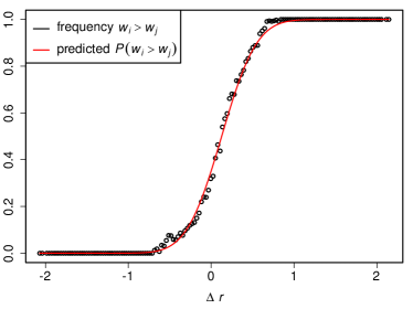
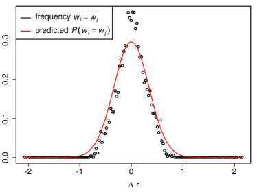
(a) normal distribution $F$

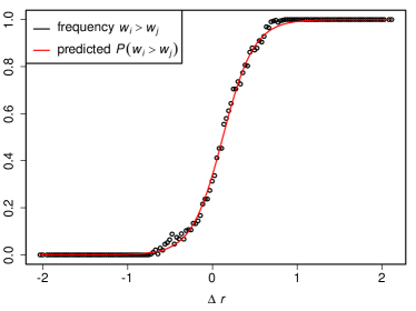
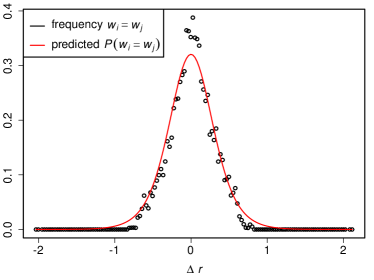
(b) logistic distribution $F$

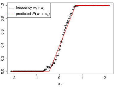
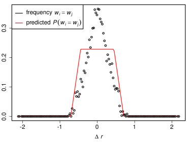
(c) uniform distribution $F$

Figure 3: Comparison of the observed relative frequencies with the probabilities predicted by model (1) for 150 bins $\Delta r=r_{i}-r_{j}$ and scores estimated by non-linear least squares (LSQ).

4.1 Goodness of fit

Both the ML method and the LSQ method yield estimators for the sentiment scores $r_{i}$ even in cases where the model assumptions in Eq. (1) do not hold. It is thus necessary to verify that the model explains the experimental observations. Moreover, it is also interesting to check which of the six solutions (three different distributions functions in combination with ML or LSQ) provides the best fit to the experimental data.

A visual way to verify the model consists in cutting the possible score differences $\Delta r=r_{i}-r_{j}$ into bins and to compare the observed frequencies for $w_{i}>w_{j}$ and $w_{i}\approx w_{j}$ with the probabilities (1) predicted by the model. The resulting plots for the LSQ estimates are shown in Fig. 3. The figures show that the model indeed predicts the observed frequencies, albeit better for wins or losses than for draws. This is no surprise because only one fourth of the comparisons were draws and consequently the ML or LSQ estimation step fits the scores rather to the winning probability than to the draw probability.

	$G=600$				$G=800$
	LSQ		ML		LSQ		ML
	$\chi^{2}$	$p$	$\chi^{2}$	$p$	$\chi^{2}$	$p$	$\chi^{2}$	$p$
normal	$1151$	$0.001$	$1286$	$1.6\cdot 10^{-9}$	$1450$	$0.169$	$1541$	$0.005$
logistic	$1027$	$0.262$	$1192$	$2.2\cdot 10^{-5}$	$1335$	$0.887$	$1511$	$0.019$
uniform	$\infty$	$0.000$	$5218$	$0.000$	$\infty$	$0.000$	$5415$	$0.000$
$\chi^{2}_{1-\alpha}$	$1074$				1487

Table 1: Goodness-of-fit test statistic $\chi^{2}$ and $p$-values $P(\mbox{\em value}>\chi^{2})$ for the different score estimators. The last row gives the corresponding threshold for rejecting the null hypothesis that the model produced the result at a significance level $\alpha=0.05$.

For a more formal goodness-of-fit test, we computed the $\chi^{2}$ statistic which is the sum of the squared differences between the expected and observed frequencies. For our paired comparison model, it reads [28]

$$\chi^{2}=\sum_{g=1}^{G} \left(\frac{(W_{g}-E(W_{g}))^{2}}{E(W_{g})}\right.+$$ (14)

$$\left.\quad\frac{(D_{g}-E(D_{g}))^{2}}{E(D_{g})}+\frac{(L_{g}-E(L_{g}))^{2}}{E(L_{g})}\right)$$

where $G$ is the number of bins $I_{1},\ldots,I_{G}$ into which the $\Delta r=r_{i}-r_{j}$ are grouped, and $W_{g}$, $D_{g}$, and $L_{g}$ are the number of wins, draws, or losses in each group. The expected number of wins, draws, or losses are computed as the sum of the respective probabilities according to the model (1), e.g.

$$E(W_{g}) =\sum_{\Delta r\in I_{g}}F(\Delta r-t)\quad\mbox{ and }$$ (15)

$$E(D_{g}) =\sum_{\Delta r\in I_{g}}\Big{(}F(\Delta r+t)-F(\Delta r-t)\Big{)}$$ (16)

The statistic (14) is approximately $\chi^{2}$ distributed when the number of members in each group is not too small. The number of degrees of freedom is $2G-n-2$, because out of the three possible outcomes in each group only two are a free choice (when the outcome is neither win nor draw, it must be a loss) and there are $n+1$ fitted parameters in the model: the $n$ ratings $r_{i}$ and the draw width $t$.

Douglas suggested in [28] to use each possible score difference as its own group, but this would mean that we would only have two items per group and the test statistic would not be $\chi^{2}$ distributed. We therefore formed the groups as quantiles among the $|\Delta r|$ values such that each group had approximately the same number of samples, a method commonly deployed in testing logistic regressions [29].

The resulting $\chi^{2}$ values are listed in Table 1. Surprisingly, the LSQ estimators lead to a clearly better goodness-of-fit than the ML estimators, with the ML estimators even yielding such a high value for $\chi^{2}$ that the model would be rejected as unlikely. As usual for $\chi^{2}$ tests, the result varies with the number of groups however, and the $p$-values are different for different numbers of groups $G$. Nevertheless, the relative values of $\chi^{2}$ for fixed $G$ allow to compare different estimation methods, and in all cases the LSQ estimator yielded a clearly better fit. With respect to the distribution function $F$, the uniform distribution provides an impossible LSQ fit because it leads to wins with zero probability in some groups. $\chi^{2}$ is smallest for the logistic choice for $F$, which is therefore the model which conforms best to the observed test person answers.

We conclude that, for estimating the sentiment scores, the non-linear LSQ estimators given by Eqs. (8) and (12) should be used.

4.2 Score values

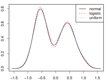
Figure 4: Kernel density plot of the polarity score distribution in our sentiment lexicon, estimated with non-linear LSQ for different cumulative distribution functions $F$.

	normal	logistic	uniform
unpraktisch (unpractical)	-0.378	-0.396	-0.344
rüde (uncouth)	-0.628	-0.629	-0.631
t (draw width)	0.126	0.122	0.132
$P(\mbox{unpraktisch}>\mbox{r\"{u}de})$	0.644	0.647	0.635
$P(\mbox{unpraktisch}\approx\mbox{r\"{u}de})$	0.226	0.227	0.228

Table 2: Comparison of scores obtained for different distribution functions $F$.

For the 199 different words, we estimated the polarity scores with the LSQ method with the three distribution functions of Fig. 1. The draw width $t$ turned out to be 0.126 for the normal distribution, 0.122 for the logistic distribution, and 0.132 for the uniform distribution. Fig. 4 shows a kernel density plot [30] for the resulting score distributions. The valley around zero (neutrality) is due to the fact that the words were drawn from the SentiWS data, which only contains positive or negative words. The comparative shapes are as expected from Fig. 1: the slightly steeper slope of the logistic distribution $F(x)$ at $x=0$ leads to a slightly stronger separation of the positive and negative scores. The range of the score values depends on the distribution $F$, too: for the normal distribution it is $[-1.058,1.099]$, for the logistic distribution $[-1.042,1.083]$, and for the uniform distribution $[-1.080,1.118]$. The example in Table 2 shows that the varying difference in ratings for the different distribution functions has only little effect on the “winning probabilities”, because the greater rating difference for the uniform distribution, e.g., is compensated by its greater draw width $t$.

adjective	$r_{\mbox{\scriptsize\em direct}}$	$r_{\mbox{\scriptsize\em paired}}$	$\sigma_{\mbox{\scriptsize\it boot}}$
paradiesisch (paradisaical)	1.00	0.966	0.039
wunderbar (wonderful)	1.00	0.915	0.045
perfekt (perfect)	0.95	1.083	0.057
traumhaft (dreamlike)	0.95	1.041	0.050
prima (great)	0.75	0.793	0.041
zufrieden (contented)	0.75	0.613	0.034
kinderleicht (easy-peasy)	0.50	0.462	0.034
lebensfähig (viable)	0.50	0.351	0.032
ausgeweitet (expanded)	0.05	-0.012	0.027
verbindlich (binding)	0.00	0.143	0.023
kontrovers (controversial)	-0.05	-0.268	0.029
unpraktisch (unpractical)	-0.50	-0.396	0.026
rüde (uncouth)	-0.50	-0.629	0.026
falsch (wrong)	-0.75	-0.627	0.025
unbarmherzig (merciless)	-0.75	-0.772	0.027
erbärmlich (wretched)	-1.00	-0.804	0.025
tödlich (deadly)	-1.00	-1.042	0.031

Table 3: Example scores from average direct assignment and paired comparisons with the logistic distribution.

It is interesting to compare the scores from paired comparisons for words which have obtained the same score from direct assignment on the five grade scale. The examples in table 3 show that the paired comparisons indeed lead to a different and finer rating scheme than averaging over coarse polarity scores from direct assignments, and that they even can lead to a reversed rank order (see, e.g., “traumhaft” and “wunderbar”). We have also estimated the variances of the polarity score estimates as the bootstrap variance $\sigma_{\mbox{\scriptsize\it boot}}^{2}$ from 200 bootstrap replications of all paired results [31]. These can be used to test whether, for $r_{i}\neq r_{j}$, the score difference is significant by computing the $p$-value $1-\Phi\left(|r_{i}-r_{j}|/\sqrt{\sigma_{i}^{2}+\sigma_{j}^{2}}\right)$, where $\Phi$ is the distribution function of the standard normal distribution. For the words “unpraktisch” and “rüde”, e.g., the $p$-value is much less than 5% and the difference is therefore statistically significant, although they obtained identical scores on the five grade scale from direct estimation.

4.3 Adding new words

To obtain a lower bound for the error in estimating scores for unknown words, we have first computed the scores for all words with the estimators for one unknown rating $r$ as described in section 2.1, where each word was compared with all other words and the scores $q_{i}$ for other words were considered to be known from the results in the preceding section. For the logistic distribution, the mean absolute error with respect to the non-linear LSQ score was much higher for the maximum-likelihood estimator ($0.012$) than for method-of-moments estimator ($<10^{-5}$) computed with Eq. (4). This was to be expected because the “ground truth score” was also based on the difference between observed and expected wins and draws. With respect to the ML score, the ML estimator was better ($0.002$ versus $0.012$), but, as we have seen in section 4.1, the ML scores are a much poorer model fit and therefore should not be used as a point of reference. We therefore have used the method-of-moments estimator (4) in our evaluations.

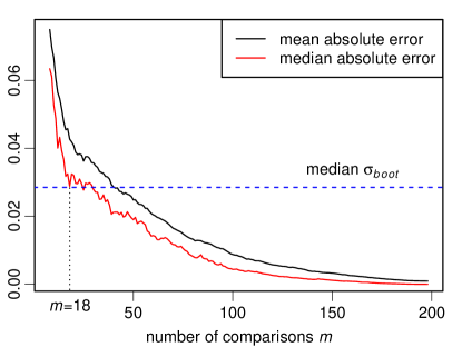
Figure 5: Mean and median absolute error from leave-one-out as a function of the number of comparisons in Algorithm 1.

For a reasonable recommendation for the number of incomplete comparisons, we have varied the number of comparisons $m$ in a leave-one-out two-fold application of Algorithm 1 on basis of the two-fold round robin experiment. The results are shown in Fig. 5. As a point of reference, the median of the bootstrap standard deviation $\sigma_{\mbox{\scriptsize\it boot}}$ of the ground truth scores is given too ($0.029$). The median of the absolute score errors reaches this reference value first for $m=18$, which corresponds to picking $m-\log_{2}(n)\approx 10$ neighbors after Silverstein & Farrel’s method.

To check whether our word selection method based on Silverstein & Farrel’s method actually is an improvement over picking words for comparison at random, we did a 100-fold Monte-Carlo experiment with choosing $18$ words at random and computing from all corresponding two-fold comparisons the method-of-moments score estimate. This yielded on average a mean error of $0.067$ and a median error $0.053$, which are considerably greater than the errors of Algorithm 1. We therefore conclude that incomplete comparisons with only 18 out of 199 words yield a reasonably accurate score estimate, provided the words are selected with our method.

4.4 Comparison to corpus-based lexica

The polarity scores computed in our experiments provide nice ground truth data for the evaluation of corpus-based polarity scores. We therefore compared the scores from SentiWS 1.8, SenticNet 3.0, SenticNet 4.0, and SentiWordNet 3.0 with the scores computed from test persons’ paired comparisons. SenticNet and SentiWordNet only contain English words, from which we have computed scores for the German words by translating each German word with both of the German-English dictionaries from www.dict.cc and www.freedict.org and by averaging the corresponding scores, a method that we call “averaged translation”.

A natural measure for the closeness between lists of polarity scores is Pearson’s correlation coefficient $r_{p}$, which has the advantage that it is invariant both under scale and translation of the variables. This is crucial in our case, because score values from paired comparisons allow for arbitrary shift and scale as explained in section 2. $r_{p}$ is highest for a linear relationship and smaller for other monotonous relationships. As can be seen in Table 4, this means that its value depends on the shape of the model distribution function $F$, albeit only slightly. Whatever function is used, the correlation between the scores from direct assignment and paired comparison is very strong. This was to be expected, because both values stem from the same test persons.

	choice for $F$
	normal	logistic	uniform
direct	$0.977$	$0.978$	$0.973$
SentiWS	$0.714$	$0.715$	$0.713$
SenticNet 3.0	$0.759$	$0.763$	$0.752$
SenticNet 4.0	$0.824$	$0.828$	$0.817$
SentiWordNet 3.0	$0.792$	$0.794$	$0.789$

Table 4: Pearson Correlation $r_{p}$ of the parity scores from the paired comparison with that of direct assignment and corpus-based methods.

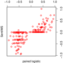
(a) SentiWS

(b) SenticNet 3.0

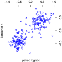
(c) SenticNet 4.0

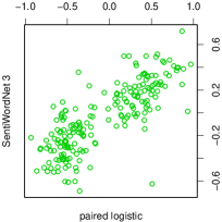
(d) SentiWordNet 3.0

Figure 6: Scatter plots comparing corpus-based scores with scores from paired comparisons.

From the corpus based lexica, the correlation with the paired scores is highest for SenticNet 4.0. According to the significance tests in the R package cocor [32], the difference to the correlation of SentiWordNet is not statistically significant at a 5% significance level, but it is significant with respect to the other two corpus based lexica, including SenticNet 3.0.

Another comparison criterion that is in favor of SenticNet 4.0 can be seen in Fig. 7: the bimodal shape of the score distribution is only reflected in the SenticNet scores. SentiWordNet has an unimodal score distribution centered around zero, and SentiWS has many identical scores with values $0.0040$ and $-0.0048$, which show up as horizontal lines in Fig. 6(a). This peculiar distribution of the SentiWS scores was also reported in the original paper presenting the SentiWS data set by Remus et al. (see Fig. 1 in [5]). The identical scores show up in Fig. 7 as a peak around neutrality, which corresponds to a valley (sic!) in the score distribution from paired comparisons.

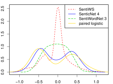
Figure 7: Kernel density plots of the polarity score distributions. The paired comparison scores have been scaled to the range $[-1,1]$.

As an alternative to our “averaged translation” approach, the third party Python module senticnetapi also provides sentiment scores for German words, which cannot be recommended, however. These have been obtained from SenticNet 4.0 by automatic translation from English to German, which is the reverse direction than our approach. This has the effect that only 35% of the words in our lexicon have matches in senticnetapi, and these only have a correlation of $0.694$, which is even less than the value for SentiWS.

Based on these observations, we consider the polarity scores from SenticNet 4.0 the most reliable among the investigated corpus based lexica. For foreign languages, we recommend to translate from the foreign language to English and compute the mean score among the matches, rather than to translate from English into the foreign language.

5 Conclusions

The new sentiment lexicon from paired comparison is a useful resource that can be used for different aims. It can be used, e.g., as ground truth data for testing and comparing automatic corpus-based methods for building sentiment lexica, as we did in section 4.4. Our results suggest that the most reliable corpus-based sentiment lexicon, among the tested ones, is SenticNet 4.0. When it is used with non-English languages, the “averaged translation” method should be used rather than a translation from English into the foreign language.

Our lexicon can also be used as a starting point for building specialized lexica for polarity studies. The method for adding new words makes the method of paired comparison applicable to studies with an arbitrary vocabulary because it yields accurate polarity scores even for rare words. We make our new lexicon, a GUI for adding words via test users, and the software for computing scores freely available on our website.

Although our results suggest that only $18$ two-fold comparisons are sufficient for estimating the score of a new, yet unknown word, this is still very time-consuming in practice. It would thus be interesting to combine the paired-comparison method with a corpus-based lexicon, such that only missing words or words estimated with a low confidence are added by experiments with test persons. Such a hybrid approach would be an interesting subject for further research.

References

- [1] S. Kiritchenko, X. Zhu, and S. M. Mohammad, “Sentiment analysis of short informal texts,” Journal of Artificial Intelligence Research, pp. 723–762, 2014.
- [2] W. Khiari, M. Roche, and A. B. Hafsia, “Integration of lexical and semantic knowledge for sentiment analysis in sms,” in Proceedings of the Tenth International Conference on Language Resources and Evaluation (LREC 2016), pp. 1185–1189, 2016.
- [3] K. Morik, A. Jung, J. Weckwerth, S. Rötner, S. Hess, S. Buschjäger, and L. Pfahler, “Untersuchungen zur Analyse von deutschsprachigen Textdaten,” Tech. Rep. 02/2015, Technische Universität Dortmund, 2015.
- [4] K. W. Church and P. Hanks, “Word association norms, mutual information, and lexicography,” Computational linguistics, vol. 16, no. 1, pp. 22–29, 1990.
- [5] R. Remus, U. Quasthoff, and G. Heyer, “SentiWS - a publicly available German-language resource for sentiment analysis,” in Conference on Language Resources and Evaluation (LREC), pp. 1168–1171, 2010.
- [6] S. Baccianella, A. Esuli, and F. Sebastiani, “SentiWordNet 3.0: An enhanced lexical resource for sentiment analysis and opinion mining.,” in International Conference on Language Resources and Evaluation (LREC), vol. 10, pp. 2200–2204, 2010.
- [7] E. Cambria, D. Olsher, and D. Rajagopal, “SenticNet 3: A common and common-sense knowledge base for cognition-driven sentiment analysis,” in AAAI conference on artificial intelligence, pp. 1515–1521, 2014.
- [8] E. Cambria and A. Hussain, Sentic Computing: A Common-Sense-Based Framework for Concept-Level Sentiment Analysis. Cham, Switzerland: Springer, 2015.
- [9] E. Cambria, S. Poria, R. Bajpai, and B. Schuller, “SenticNet 4: A semantic resource for sentiment analysis based on conceptual primitives,” in the 26th International Conference on Computational Linguistics (COLING), Osaka, pp. 2666–2677, 2016.
- [10] T. Wilson, J. Wiebe, and P. Hoffmann, “Recognizing contextual polarity in phrase-level sentiment analysis,” in Conference on human language technology and empirical methods in natural language processing (HTL/EMNLP), pp. 347–354, 2005.
- [11] M. Wiegand, C. Bocionek, A. Conrad, J. Dembowski, J. Giesen, G. Linn, and L. Schmeling, “Saarland University’s participation in the German sentiment analysis shared task (GESTALT),” in Workshop Proceedings of the 12th KONVENS, pp. 174–184, 2014.
- [12] R. K. Mantiuk, A. Tomaszewska, and R. Mantiuk, “Comparison of four subjective methods for image quality assessment,” Computer Graphics Forum, vol. 31, no. 8, pp. 2478–2491, 2012.
- [13] A. E. Elo, The Rating of Chess Players, Past and Present. New York: Arco, 1978.
- [14] W. H. Batchelder and N. J. Bershad, “The statistical analysis of a Thurstonian model for rating chess players,” Journal of Mathematical Psychology, vol. 19, no. 1, pp. 39–60, 1979.
- [15] D. A. Silverstein and J. E. Farrell, “Efficient method for paired comparison,” Journal of Electronic Imaging, vol. 10, no. 2, pp. 394–398, 2001.
- [16] K. Denecke, “Using SentiWordNet for multilingual sentiment analysis,” in International Conference on Data Engineering Workshop, pp. 507–512, 2008.
- [17] M. Korayem, K. Aljadda, and D. Crandall, “Sentiment/subjectivity analysis survey for languages other than english,” Social Network Analysis and Mining, vol. 6, no. 1, p. 75, 2016.
- [18] C. Dalitz and K. E. Bednarek, “Sentiment lexica from paired comparisons,” in International Conference on Data Mining Workshops (ICDMW), pp. 924–930, 2016.
- [19] C. Dalitz, “Corrigendum to: Sentiment lexica from paired comparisons,” Tech. Rep. 2017-02, Hochschule Niederrhein, Fachbereich Elektrotechnik und Informatik, 2017.
- [20] L. L. Thurstone, “A law of comparative judgment.,” Psychological Review, vol. 34, no. 4, pp. 368–389, 1927.
- [21] M. Cattelan, “Models for paired comparison data: A review with emphasis on dependent data,” Statistical Science, vol. 27, no. 3, pp. 412–433, 2012.
- [22] R. A. Bradley and M. E. Terry, “Rank analysis of incomplete block designs: I. the method of paired comparisons,” Biometrika, vol. 39, no. 3/4, pp. 324–345, 1952.
- [23] G. E. Noether, “Remarks about a paired comparison model,” Psychometrika, vol. 25, no. 4, pp. 357–367, 1960.
- [24] H. Stern, “Are all linear paired comparison models empirically equivalent?,” Mathematical Social Sciences, vol. 23, no. 1, pp. 103–117, 1992.
- [25] M. Vojnovic and S. Yun, “Parameter estimation for generalized thurstone choice models,” in International Conference on Machine Learning, pp. 498–506, 2016.
- [26] T. V. Elzhov, K. M. Mullen, A.-N. Spiess, and B. Bolker, minpack.lm: R Interface to the Levenberg-Marquardt Nonlinear Least-Squares Algorithm Found in MINPACK, 2016. R package version 1.2-1.
- [27] A. Esuli and F. Sebastiani, “SentiWordNet: A publicly available lexical resource for opinion mining,” in International Conference on Language Resources and Evaluation (LREC), pp. 417–422, 2006.
- [28] G. A. Douglas, “Goodness of fit tests for paired comparison models,” Psychometrika, vol. 43, no. 1, pp. 129–130, 1978.
- [29] D. W. Hosmer and S. Lemesbow, “Goodness of fit tests for the multiple logistic regression model,” Communications in statistics-Theory and Methods, vol. 9, no. 10, pp. 1043–1069, 1980.
- [30] S. Sheather and M. Jones, “A reliable data-based bandwidth selection method for kernel density estimation,” Journal of the Royal Society series B, vol. 53, pp. 683–690, 1991.
- [31] B. Efron and R. Tibshirani, “Bootstrap methods for standard errors, confidence intervals, and other measures of statistical accuracy,” Statistical Science, pp. 54–75, 1986.
- [32] B. Diedenhofen and J. Musch, “cocor: A comprehensive solution for the statistical comparison of correlations,” PLoS ONE, vol. 10, no. 4, p. e0121945, 2015.