Fully-coupled pressure-based algorithm for compressible flows:
linearisation and iterative solution strategies

Abstract

The impact of different linearisation and iterative solution strategies for fully-coupled pressure-based algorithms for compressible flows at all speeds is studied, with the aim of elucidating their impact on the performance of the numerical algorithm. A fixed-coefficient linearisation and a Newton linearisation of the transient and advection terms of the governing nonlinear equations are compared, focusing on test-cases that feature acoustic, shock and expansion waves. The linearisation and iterative solution strategy applied to discretise and solve the nonlinear governing equations is found to have a significant influence on the performance and stability of the numerical algorithm. The Newton linearisation of the transient terms of the momentum and energy equations is shown to yield a significantly improved convergence of the iterative solution algorithm compared to a fixed-coefficient linearisation, while the linearisation of the advection terms leads to substantial differences in performance and stability at large Mach numbers and large Courant numbers. It is further shown that the consistent Newton linearisation of all transient and advection terms of the governing equations allows, in the context of coupled pressure-based algorithms, to eliminate all forms of underrelaxation and provides a clear performance benefit for flows in all Mach number regimes.

textheight=25cm, textwidth=16cm

1 Introduction

The accurate and robust simulation of compressible flows across different Mach number regimes using the same numerical framework is a widely sought objective that is notoriously difficult to achieve. The main problems associated with devising numerical algorithms for flows in all Mach number regimes are finding suitable discrete formulations that account for the change in mathematical character of the governing conservation laws, including the related change in the thermodynamic meaning of pressure and density, and the fully-conservative discretisation of the governing conservation laws [1, 2].

A straightforward discretisation of the governing conservation laws leads to density-based algorithms [3, 4, 5], where density is the solution variable associated with the conservation of mass, that are particularly suited for flows in which compressible effects are significant. However, density-based algorithms are ill-suited for flows with low Mach numbers [5, 2, 6, 7, 8], where the natural coupling between density and pressure is weak. Consequently, the continuity equation is no longer effective as a transport equation for density but instead becomes a constraint on the velocity field. The problems associated with density-based algorithms at low Mach numbers and the desire to be able to simulate flows at all speeds with the same numerical framework have motivated the development of pressure-based algorithms [9, 10, 11, 12, 8], in which the continuity equation serves as an equation for pressure, while density is evaluated explicitly using a suitable equation of state. In the low Mach number regime, pressure is strongly coupled to velocity, while the pressure-density coupling is negligible; in the hypersonic flow regime, pressure is strongly coupled to density, while the pressure-velocity coupling is negligible. This dual role of pressure facilitates the success of pressure-based methods in solving flows in all Mach number regimes [10, 12, 13]. However, pressure-based algorithms exhibit stability and convergence issues when both the pressure-velocity and the pressure-density coupling are significant simultaneously, in particular in the transonic flow regime [2], due to the strong coupling and nonlinearity of the governing equations.

Starting with the seminal work of Harlow and Amsden [14, 9], a large number and varieties of segregated [15, 10, 16, 17, 18, 8] and coupled [11, 19, 20, 21, 22, 23, 24] pressure-based algorithms have been proposed for compressible single-phase flows. Among the available segregated methods, the class of SIMPLE [10, 16, 17, 18] and PISO [15, 17, 18] methods are most widely used, providing good performance with low computational resources, in particular computer memory. The key shortcoming of segregated methods for compressible flows is the weak pressure-velocity-density coupling of the discretised governing equations as a result of the segregated [25, 23], iterative predictor-corrector solution procedure, which necessitates underrelaxation of the discretised equations to reach a converged solution. The simultaneous solution of the governing equations by coupled methods, in which all discretised governing equations are solved in a single system of equations using implicit solution methods, more closely represents their strongly coupled nature. Although coupled methods typically require larger computational resources for the solution of the linear system of discretised governing equations than segregated methods, they benefit from an improved convergence and robustness [11, 23], in particular on large computational meshes and for complex flows. Recently, Xiao et al. [24] proposed a coupled pressure-based algorithm with a dual-loop solution procedure to circumvent explicit underrelaxation, featuring an inner iteration loop in which density is updated assuming the flow is barotropic, with which stable convergence has been demonstrated for flows in all Mach number regimes [24].

A point of particular interest when developing numerical algorithms for strongly nonlinear phenomena, such as compressible flows, is the type of linearisation applied to the nonlinear governing equations. A well-suited linearisation strategy can provide a substantial increase in performance and stability of the numerical algorithm [26, 1, 25, 2]. Two linearisation methods that are particularly popular and widely applied in numerical algorithms to predict fluid flows are the fixed-coefficient linearisation (or “lagging” the coefficients) and the Newton linearisation (also known as Newton-Raphson method). In the fixed-coefficient linerisation, only the primary solution variable is solved implicitly, while all coefficients are computed based on known information. For a generic primary variable $\phi$ with its variable coefficient $\alpha$, the nonlinear term $\alpha^{(n+1)}\,\phi^{(n+1)}$ to be solved, with $n$ the iteration counter, is approximated as

$$\alpha^{(n+1)}\phi^{(n+1)}\approx\alpha^{(n)}\phi^{(n+1)}\ ,$$ (1)

where superscript $(n)$ denotes the most recent available solution. In the context of pressure-based algorithms, arguments for a fixed-coefficient linearisation are its easy implementation, and that it is not necessary to treat the fluxes and the density implicitly as a function of one of the primary solution variables. The Newton linearisation is an often chosen alternative to the fixed-coefficient linearisation, see e.g. [27, 23, 24], providing superior convergence rates and stability of the solution algorithm [2], as for instance demonstrated by Kunz et al. [25] in the context of a coupled pressure-based multi-fluid Euler-Euler method. Applying a Newton linearisation, the nonlinear term $\alpha^{(n+1)}\,\phi^{(n+1)}$ is approximated as

$$\begin{split}\alpha^{(n+1)}\phi^{(n+1)}&\approx\alpha^{(n)}\phi^{(n)}+\left(\alpha^{(n+1)}-\alpha^{(n)}\right)\left.\frac{\partial\alpha\phi}{\partial\alpha}\right|^{(n)}+\left(\phi^{(n+1)}-\phi^{(n)}\right)\left.\frac{\partial\alpha\phi}{\partial\phi}\right|^{(n)}\\ &=\alpha^{(n)}\phi^{(n+1)}+\alpha^{(n+1)}\phi^{(n)}-\alpha^{(n)}\,\phi^{(n)}\ .\end{split}$$ (2)

Arguments in support of the Newton linearisation for simulating compressible flows typically point to a suitable treatment and smooth transition from elliptic/parabolic to hyperbolic behaviour of the governing equations [20, 28, 24], in particular the continuity equation, in different Mach number regimes, as well as an implicit contribution of additional active flow-dependent variables, such as the fluxes. Despite the often stated importance of the applied linearisation for the performance and robustness of the solution algorithm in the relevant literature, notably textbooks [1, 2, 29], a systematic study of the linearisation for pressure-based algorithms for compressible flows has not been published to date.

In this article, the linearisation of the governing equations as well as the iterative solution strategy for a fully-coupled pressure-based algorithm for the simulation of flows at all speeds, based on the framework proposed by Xiao et al. [24], is studied. Considering the fixed-coefficient and Newton linearisations, the different possible linearisation strategies for each term of the governing equations are studied and the resulting performance and stability of the numerical algorithm are compared using representative test-cases in all Mach number regimes, including the propagation of acoustic waves, shock tubes and supersonic flows over a forward-facing step and a circular cone. The presented results demonstrate subtle differences between the considered linearisation strategies and highlight the importance of a careful linearisation of the governing nonlinear equations. The execution times for all presented simulations are given together with the used computational hardware, as a reference for future algorithm development and comparisons.

The governing equations are briefly introduced in Section 2 and the applied numerical framework is presented in Section 3. The considered linearisation techniques and solution procedures are discussed in Section 4 and the results of representative test-cases are presented in Section 5. The findings are summarised and the article is concluded in Section 6.

2 Governing equations

The considered compressible flows of an inviscid fluid are governed by the continuity, momentum and energy equations, given as (using the Einstein notation)

$$\frac{\partial\rho}{\partial t}+\frac{\partial\rho u_{i}}{\partial x_{i}} =0\ ,$$ (3)

$$\frac{\partial\rho u_{j}}{\partial t}+\frac{\partial\rho u_{i}u_{j}}{\partial x_{i}} =-\frac{\partial p}{\partial x_{j}}\ ,$$ (4)

$$\frac{\partial\rho h}{\partial t}+\frac{\partial\rho u_{i}h}{\partial x_{i}} =\frac{\partial p}{\partial t}\ ,$$ (5)

respectively, where $t$ is time, $\boldsymbol{x}$ the Cartesian coordinates, $\rho$ is the density, $\boldsymbol{u}$ is the velocity vector, $p$ is the pressure and $h=c_{p}\,T+\boldsymbol{u}^{2}/2$ is the specific total enthalpy, with $c_{p}$ the specific isobaric heat capacity and $T$ the temperature. For simplicity, but without loss of generality, viscous stresses, heat conduction and external forces are neglected in this study. The system of governing equations is closed by the ideal gas equation of state

$$\rho=\frac{p}{(\gamma-1)\,c_{v}\,T}\ ,$$ (6)

where $c_{v}$ is the specific isochoric heat capacity and $\gamma=c_{p}/c_{v}$ is the heat capacity ratio. The speed of sound is given as

$$a=\sqrt{\frac{\gamma\,p}{\rho}}\ .$$ (7)

3 Numerical framework

A coupled pressure-based finite-volume framework for compressible flows, based on the numerical framework of Xiao et al. [24], is employed to solve the governing equations. This numerical framework is founded on a collocated variable arrangement, is applicable to unstructured meshes and does not apply any explicit underrelaxation to the iterative solution algorithm. In this section, the discretisation and implementation of the governing equations is explained, focusing on the methods and ingredients relevant to this study. Further details on the applied finite-volume framework can be found in previous work [24]. The considered linearisation and solution strategies are discussed in Section 4.

3.1 Spatial and temporal discretisation

The central differencing scheme is applied for the interpolation from cell centres to face centres of variables that are not advected, given for a general flow variable $\phi$ at face $f$, see Fig. 1, as

$$\overline{\phi}_{f}=\frac{\phi_{P}+\phi_{Q}}{2}\ .$$ (8)

Advected variables are interpolated to face centres using the Minmod scheme [30], with the face value following as

$$\tilde{\phi}_{f}=\phi_{U}+\frac{\xi_{f}}{2}(\phi_{D}-\phi_{U})\ ,$$ (9)

where subscripts $U$ and $D$ denote the upwind and downwind cells, and $\xi_{f}$ is the flux limiter. Other TVD schemes would be equally applicable but are not considered as part of this study.

Figure 1: Schematic illustration of cell $P$ with its neighbour cell $Q$ and the shared face $f$, where $\boldsymbol{n}_{f}$ is the unit normal vector of face $f$ (outward pointing with respect to cell $P$).

The First-Order Backward Euler and the Second-Order Backward Euler schemes are applied for the discretisation of transient terms, given for cell $P$ as

$$\int_{V_{P}}\frac{\partial\phi}{\partial t}\ dV\approx\frac{\phi_{P}-\phi_{P}^{(t-\Delta t)}}{\Delta t}\,V_{P}$$ (10)

and

$$\int_{V_{P}}\frac{\partial\phi}{\partial t}\ dV\approx\frac{3\phi_{P}-4\phi_{P}^{(t-\Delta t)}+\phi_{P}^{(t-2\Delta t)}}{2\Delta t}\,V_{P}\ ,$$ (11)

respectively, where $\Delta t$ is the applied time-step, superscripts $(t-\Delta t)$ and $(t-2\Delta t)$ denote values of the previous time-level and the previous-previous time-level, respectively, and $V_{P}$ is the volume of cell $P$. For simplicity, the discretised governing equations are presented below using the First-Order Backward Euler scheme, but the Second-Order Backward Euler scheme is also applied as part of this study. In the interest of consistency, all transient terms of the governing equations are always discretised with identical schemes.

3.2 Advecting velocity

At cell faces $f$, an advecting velocity $\vartheta_{f}=\boldsymbol{u}_{f}\boldsymbol{n}_{f}$ is defined using the momentum-weighted interpolation method, with $\boldsymbol{n}_{f}$ the unit normal vector of face $f$. This advecting velocity takes the role of flux-velocity in the discretised advection terms of the governing equation. Following the work of Xiao et al. [24], the advecting velocity $\vartheta_{f}$ at face $f$ is defined as

$$\vartheta_{f}\approx\overline{u}_{f,i}\,n_{f,i}-\hat{d}_{f}\left[\left.\frac{\partial p}{\partial x_{i}}\right|_{f}n_{f,i}-\frac{1}{2}\left(\left.\frac{\partial p}{\partial x_{i}}\right|_{P}+\left.\frac{\partial p}{\partial x_{i}}\right|_{Q}\right)n_{f,i}\right]+\hat{d}_{f}\frac{\rho_{f}^{(t-\Delta t)}}{\Delta t}\left(\vartheta^{(t-\Delta t)}_{f}-\overline{u}^{(t-\Delta t)}_{f,i}\,n_{f,i}\right)\,,$$ (12)

where $\overline{\boldsymbol{u}}_{f}$ is obtained by linear interpolation from the values at the adjacent cell centres and

$$\left.\frac{\partial p}{\partial x_{i}}\right|_{f}n_{f,i}\approx\frac{p_{Q}-p_{P}}{\Delta x}\ .$$ (13)

The coefficient $\hat{d}_{f}$ follows directly from the coefficients of the advection terms (and, if considered, viscous stress terms) of the momentum equations, see for instance [31]. This formulation of the advecting velocity provides a robust pressure-velocity coupling at all Mach numbers [24]. For low Mach numbers and incompressible flows, the pressure term acts as a low-pass filter on high-order derivatives of pressure [32, 2, 29], because

$$\left.\frac{\partial p}{\partial x_{i}}\right|_{f}-\frac{1}{2}\left(\left.\frac{\partial p}{\partial x_{i}}\right|_{P}+\left.\frac{\partial p}{\partial x_{i}}\right|_{Q}\right)\propto\left.\frac{\partial^{3}p}{\partial x_{i}^{3}}\right|_{f}\ ,$$ (14)

which damps pressure oscillations arising as a result of pressure-velocity decoupling in a collocated variable arrangement.

3.3 Discretised governing equations

Applying the First-Order Backward Euler scheme (chosen here for demonstration), given by Eq. (10), for the discretisation of the transient terms and the advecting velocity $\vartheta_{f}$, given by Eq. (12), in the advection terms, the discretised continuity equation (3) for mesh cell $P$ is given as

$$\frac{\rho_{P}^{(n+1)}-\rho_{P}^{(t-\Delta t)}}{\Delta t}\,V_{P}+\sum_{f}\tilde{\rho}_{f}\vartheta_{f}A_{f}=0\ ,$$ (15)

where $A_{f}$ is the area of face $f$. For all results presented as part of this study, the cell-centred density $\rho_{P}^{(n+1)}$ in the transient term of the continuity equation is formulated as an implicit function of pressure $p$, given as

$$\rho^{(n+1)}_{P}=\frac{p^{(n+1)}_{P}}{(\gamma-1)\,c_{v}\,T_{P}}\ ,$$ (16)

where $T$ is the most recent available temperature value, which is dependent on the applied solution procedure and is detailed in Section 4.3. The linearisation of the advection term of Eq. (15) is discussed in Section 4.1. The discretised momentum equations (4) and energy equation (5) for mesh cell $P$ follow in a similar manner as

$$\frac{\rho_{P}u_{P,j}-\rho_{P}^{(t-\Delta t)}u_{P,j}^{(t-\Delta t)}}{\Delta t}\,V_{P}+\sum_{f}\tilde{\rho}_{f}\vartheta_{f}\tilde{u}_{f,j}A_{f} =-\sum_{f}\overline{p}_{f}n_{f,j}A_{f}\ ,$$ (17)

$$\frac{\rho_{P}h_{P}-\rho_{P}^{(t-\Delta t)}h_{P}^{(t-\Delta t)}}{\Delta t}\,V_{P}+\sum_{f}\tilde{\rho}_{f}\vartheta_{f}\tilde{h}_{f}A_{f} =\frac{p_{P}-p_{P}^{(t-\Delta t)}}{\Delta t}\,V_{P}\ ,$$ (18)

respectively. The linearisation of the transient and advection terms of Eqs. (17) and (18) is discussed in Section 4.2.

Note that the continuity, momentum and energy equations are formulated conservative in $\rho$, $\rho\boldsymbol{u}$ and $\rho h$, respectively, but are solved for the primary variables $p$, $\boldsymbol{u}$ and $h$, with $\rho$ given by Eq. (6). All cell-centred values of $p$, $\boldsymbol{u}$ and $h$ arising in the discretised governing equations are treated implicitly, which is further discussed in Section 4, and the same advecting velocity $\vartheta_{f}$ is applied in the discretised governing equations to ensure a consistent formulation of the fluxes. Van Doormaal et al. [10] and subsequent studies [11, 20, 23, 24, 31] demonstrated that choosing primitive variables instead of conserved variables as primary solution variables does not affect the conservative properties of the governing equations, if a consistent discretisation is applied. Although the continuity equation acts as a constraint on the pressure field, the resulting density and velocity fields, through the coupling with the momentum equations and the applied equation of state, satisfy the conservation of mass in all Mach number regimes [10]. The converged system of nonlinear governing equations, thus, satisfies the governing conservation laws on the discrete level.

3.4 Linear system of equations

The discretised governing equations are solved in a single linear system of equations, $\boldsymbol{A}\boldsymbol{\phi}=\boldsymbol{b}$, which for a three-dimensional flow is given as

$$\begin{pmatrix}{\boldsymbol{A}}^{u}_{\rho u}&{\boldsymbol{A}}^{v}_{\rho u}&{\boldsymbol{A}}^{w}_{\rho u}&{\boldsymbol{A}}^{p}_{\rho u}&{\boldsymbol{0}}\\ {\boldsymbol{A}}^{u}_{\rho v}&{\boldsymbol{A}}^{v}_{\rho v}&{\boldsymbol{A}}^{w}_{\rho v}&{\boldsymbol{A}}^{p}_{\rho v}&{\boldsymbol{0}}\\ {\boldsymbol{A}}^{u}_{\rho w}&{\boldsymbol{A}}^{v}_{\rho w}&{\boldsymbol{A}}^{w}_{\rho w}&{\boldsymbol{A}}^{p}_{\rho w}&{\boldsymbol{0}}\\ {\boldsymbol{A}}^{u}_{\rho\phantom{h}}&{\boldsymbol{A}}^{v}_{\rho\phantom{h}}&{\boldsymbol{A}}^{w}_{\rho\phantom{h}}&{\boldsymbol{A}}^{p}_{\rho\phantom{h}}&{\boldsymbol{0}}\\ {\boldsymbol{A}}^{u}_{\rho h}&{\boldsymbol{A}}^{v}_{\rho h}&{\boldsymbol{A}}^{w}_{\rho h}&{\boldsymbol{A}}^{p}_{\rho h}&{\boldsymbol{A}}^{h}_{\rho h}\end{pmatrix}\cdot\begin{pmatrix}\boldsymbol{\phi}^{u}\\ \boldsymbol{\phi}^{v}\\ \boldsymbol{\phi}^{w}\\ \boldsymbol{\phi}^{p}\\ \boldsymbol{\phi}^{h}\end{pmatrix}=\begin{pmatrix}\boldsymbol{b}_{\rho u}\\ \boldsymbol{b}_{\rho v}\\ \boldsymbol{b}_{\rho w}\\ \boldsymbol{b}_{\rho\phantom{h}}\\ \boldsymbol{b}_{\rho h}\end{pmatrix}\ ,$$ (19)

where $\boldsymbol{A}^{\chi}_{\zeta}$, with $\zeta$ the conserved quantity of a given governing equation and $\chi$ the solution variable, are the coefficient submatrices of the momentum equations ($\zeta=\{\rho u,\rho v,\rho w\}$), the continuity equation ($\zeta=\rho$) and the energy equation ($\zeta=\rho h$). The vectors $\boldsymbol{\phi}^{\chi}$ and $\boldsymbol{b}_{\zeta}$ are the solution subvectors and right-hand side subvectors, respectively. Note that, contrary to the work of Xiao et al. [24], the discretised energy equation is solved together with the momentum and continuity equations in the linear system of equations (19), to facilitate the implicit coupling provided by some of the studied linearisation strategies. The applied linearisation strategies, presented in Sections 4.1 and 4.2, determine the sparseness of the equation system. For the results presented in this study, the system of governing equations (19) is preconditioned and solved using the Block Jacobi preconditioner and BiCGStab solver of the PETSc library [33, 34, 35], respectively. The equation system (19) has converged if [35]

$$\|\boldsymbol{A}^{(n)}\boldsymbol{\phi}^{(n+1)}-\boldsymbol{b}^{(n)}\|<\eta\,\|\boldsymbol{b}^{(n)}\|\ ,$$ (20)

where $\eta$ is the predefined solution tolerance and $\|\cdot\|$ denotes the $L_{2}$-norm.

4 Linearisation and iterative solution strategies

Different linearisation strategies are devised by applying the fixed-coefficient linearisation, Eq. (1), and the Newton linearisation, Eq. (2), in different combinations to the various nonlinear transient terms and advection terms of the governing equations. The considered linearisation strategies are presented in Sections 4.1 and 4.2, and the applied iterative single-loop and dual-loop solution procedures are discussed in Section 4.3.

4.1 Linearisation of the continuity equation

The linearisation of the advection term of the continuity equation (15) has been discussed in several previous studies, see e.g. [10, 17, 20, 24]. The general consensus is that a Newton linearisation for this term is preferable over the fixed-coefficient linearisation, as it provides a smooth transition from the elliptic equation for pressure in the incompressible limit ($M\rightarrow 0$) to the hyperbolic nature of the continuity equation for supersonic flows ($M>1$). With different linearisations applied to the term $\rho_{f}\vartheta_{f}$, the discretised continuity equation (15) becomes

$$\frac{\rho_{P}^{(n+1)}-\rho_{P}^{(t-\Delta t)}}{\Delta t}\,V_{P}+\sum_{f}\tilde{\rho}^{(n)}_{f}\vartheta_{f}^{(n+1)}A_{f}=0$$ (21)

with the fixed-coefficient linearisation, and

$$\frac{\rho_{P}^{(n+1)}-\rho_{P}^{(t-\Delta t)}}{\Delta t}\,V_{P}+\sum_{f}\left(\tilde{\rho}^{(n)}_{f}\vartheta_{f}^{(n+1)}+\tilde{\rho}^{(n+1)}_{f}\vartheta_{f}^{(n)}-\tilde{\rho}^{(n)}_{f}\vartheta_{f}^{(n)}\right)A_{f}=0$$ (22)

with the Newton linearisation, where $\rho_{P}^{(n+1)}$ is given by Eq. (16) and $\tilde{\rho}^{(n+1)}_{f}$ is given as

$$\tilde{\rho}_{f}^{(n+1)}=\rho_{U}^{(n+1)}+\frac{\xi_{f}}{2}\left(\rho_{D}^{(n+1)}-\rho_{U}^{(n+1)}\right)\ ,$$ (23)

with $\rho_{U}^{(n+1)}$ and $\rho_{D}^{(n+1)}$ evaluated by Eq. (16). The implicit advecting velocity $\vartheta_{f}^{(n+1)}$ is given as

$$\begin{split}\vartheta_{f}^{(n+1)}\approx\overline{u}_{f,i}^{(n+1)}\,n_{f,i}&-\hat{d}_{f}\left[\frac{p_{Q}^{(n+1)}-p_{P}^{(n+1)}}{\Delta x}-\frac{1}{2}\left(\left.\frac{\partial p}{\partial x_{i}}\right|_{P}^{(n)}+\left.\frac{\partial p}{\partial x_{i}}\right|_{Q}^{(n)}\right)n_{f,i}\right]\\ &+\hat{d}_{f}\frac{\rho^{(t-\Delta t)}_{f}}{\Delta t}\left(\vartheta^{(t-\Delta t)}_{f}-\overline{u}^{(t-\Delta t)}_{f,i}\,n_{f,i}\right)\ ,\end{split}$$ (24)

where the cell-centred values of velocity and pressure are solved for implicitly, while the cell-centred pressure gradients are deferred. Preliminary studies have shown no significant differences in performance or stability for the considered test-cases when the cell-centred pressure gradients in Eq. (24) were instead treated implicitly; hence an implicit treatment of the cell-centred pressure gradients in Eq. (24) is not considered as part of this study.

For the Newton linearisation, $\tilde{\rho}_{f}^{(n)}\vartheta_{f}^{(n+1)}$ dominates over $\tilde{\rho}_{f}^{(n+1)}\vartheta_{f}^{(n)}$ for low Mach numbers, whereas $\tilde{\rho}_{f}^{(n+1)}\vartheta_{f}^{(n)}$ dominates over $\tilde{\rho}_{f}^{(n)}\vartheta_{f}^{(n+1)}$ in the hypersonic regime. Therefore, the fixed-coefficient linearisation, which is derived from a pressure-based numerical framework for incompressible flows, as discussed in [24], is expected to yield a very limited performance and stability for flows with large Mach numbers. Note that an implicit treatment of the advecting velocity is essential for a robust pressure-velocity coupling at low Mach numbers [24] and, hence, the fixed-coefficient linearisation with density as the implicit variable and the advecting velocity as the deferred coefficient is not considered in this study.

4.2 Linearisation of the momentum and energy equations

The momentum and energy equations offer more options for linearisation than the continuity equation because of the additional primary variable $\phi$, i.e. velocity $\boldsymbol{u}$ in the momentum equations (17) and specific total enthalpy $h$ in the energy equation (18). The transient term $\partial\rho u_{j}/\partial t$ of the momentum equations (17) and the transient term $\partial\rho h/\partial t$ of the energy equation (18) are linearised with the fixed-coefficient linearisation

$$\rho_{P}\phi_{P}=\rho_{P}^{(n)}\phi_{P}^{(n+1)}\ ,$$ (25)

or the Newton linearisation

$$\rho_{P}\phi_{P}=\rho_{P}^{(n)}\phi_{P}^{(n+1)}+\rho_{P}^{(n+1)}\phi_{P}^{(n)}-\rho_{P}^{(n)}\phi_{P}^{(n)}\ ,$$ (26)

with $\rho_{P}^{(n+1)}$ given by Eq. (16). Because pressure is a primary solution variable in all governing equations, no additional non-zero matrix coefficients arise when the density is treated implicitly as a function of pressure.

Applying different combinations of the fixed-coefficient and Newton linearisations, four different linearisation strategies can be devised for the advection terms of the momentum equations (17) and energy equation (18):

• Fixed-coefficient linearisation, where only the primary variable is treated implicitly,

  $$\tilde{\rho}_{f}\vartheta_{f}\tilde{\phi}_{f}=\tilde{\rho}_{f}^{(n)}\vartheta_{f}^{(n)}\tilde{\phi}_{f}^{(n+1)}\ ,$$ (27)

• Newton linearisation with respect to the density ($\rho$-Newton linearisation),

  $$\tilde{\rho}_{f}\vartheta_{f}\tilde{\phi}_{f}=\tilde{\rho}_{f}^{(n)}\vartheta_{f}^{(n)}\tilde{\phi}_{f}^{(n+1)}+\tilde{\rho}_{f}^{(n+1)}\vartheta_{f}^{(n)}\tilde{\phi}_{f}^{(n)}-\tilde{\rho}_{f}^{(n)}\vartheta_{f}^{(n)}\tilde{\phi}_{f}^{(n)}\ ,$$ (28)

• Newton linearisation with respect to the advecting velocity ($\vartheta$-Newton linearisation),

  $$\tilde{\rho}_{f}\vartheta_{f}\tilde{\phi}_{f}=\tilde{\rho}_{f}^{(n)}\vartheta_{f}^{(n)}\tilde{\phi}_{f}^{(n+1)}+\tilde{\rho}_{f}^{(n)}\vartheta_{f}^{(n+1)}\tilde{\phi}_{f}^{(n)}-\tilde{\rho}_{f}^{(n)}\vartheta_{f}^{(n)}\tilde{\phi}_{f}^{(n)}\ ,$$ (29)

• Full-Newton linearisation by combining the $\rho$-Newton and $\vartheta$-Newton linearisations,

  $$\tilde{\rho}_{f}\vartheta_{f}\tilde{\phi}_{f}=\tilde{\rho}_{f}^{(n)}\vartheta_{f}^{(n)}\tilde{\phi}_{f}^{(n+1)}+\tilde{\rho}_{f}^{(n)}\vartheta_{f}^{(n+1)}\tilde{\phi}_{f}^{(n)}+\tilde{\rho}_{f}^{(n+1)}\vartheta_{f}^{(n)}\tilde{\phi}_{f}^{(n)}-2\tilde{\rho}_{f}^{(n)}\vartheta_{f}^{(n)}\tilde{\phi}_{f}^{(n)}\ .$$ (30)

The fully linearised momentum equations (17) and energy equation (18) follow as

$$\begin{split}&\left(\overbrace{\underbrace{\rho_{P}^{(n)}u_{P,j}^{(n+1)}}_{\textup{fixed-coeff.}}+\rho_{P}^{(n+1)}u_{P,j}^{(n)}-\rho_{P}^{(n)}u_{P,j}^{(n)}}^{\textup{Newton}}-\rho_{P}^{(t-\Delta t)}u_{P,j}^{(t-\Delta t)}\right)\frac{V_{P}}{\Delta t}+\sum_{f}\overline{p}_{f}^{(n+1)}n_{f,j}A_{f}\\ &+\sum_{f}\left(\underbrace{\hbox to0.0pt{$\underbrace{\phantom{\tilde{\rho}_{f}^{(n+1)}\vartheta_{f}^{(n)}\tilde{u}_{f,j}^{(n)}-\tilde{\rho}_{f}^{(n)}\vartheta_{f}^{(n)}\tilde{u}_{f,j}^{(n)}+\tilde{\rho}_{f}^{(n)}\vartheta_{f}^{(n)}\tilde{u}_{f,j}^{(n+1)}}}_{\textup{$\rho$-Newton}}$\hss}\tilde{\rho}_{f}^{(n+1)}\vartheta_{f}^{(n)}\tilde{u}_{f,j}^{(n)}-\tilde{\rho}_{f}^{(n)}\vartheta_{f}^{(n)}\tilde{u}_{f,j}^{(n)}+\overbrace{\overbrace{\tilde{\rho}_{f}^{(n)}\vartheta_{f}^{(n)}\tilde{u}_{f,j}^{(n+1)}}^{\textup{fixed-coeff.}}+\tilde{\rho}_{f}^{(n)}\vartheta_{f}^{(n+1)}\tilde{u}_{f,j}^{(n)}-\tilde{\rho}_{f}^{(n)}\vartheta_{f}^{(n)}\tilde{u}_{f,j}^{(n)}}^{\textup{$\vartheta$-Newton}}}_{\textup{full-Newton}}\right)A_{f}=0\end{split}$$ (31)

and

$$\begin{split}&\left(\overbrace{\underbrace{\rho_{P}^{(n)}h_{P}^{(n+1)}}_{\textup{fixed-coeff.}}+\rho_{P}^{(n+1)}h_{P}^{(n)}-\rho_{P}^{(n)}h_{P}^{(n)}}^{\textup{Newton}}-\rho_{P}^{(t-\Delta t)}h_{P}^{(t-\Delta t)}\right)\frac{V_{P}}{\Delta t}-\left(p_{P}^{(n+1)}-p_{P}^{(t-\Delta t)}\right)\frac{V_{P}}{\Delta t}\\ &+\sum_{f}\left(\underbrace{\hbox to0.0pt{$\underbrace{\phantom{\tilde{\rho}_{f}^{(n+1)}\vartheta_{f}^{(n)}\tilde{h}_{f}^{(n)}-\tilde{\rho}_{f}^{(n)}\vartheta_{f}^{(n)}\tilde{h}_{f}^{(n)}+\tilde{\rho}_{f}^{(n)}\vartheta_{f}^{(n)}\tilde{h}_{f}^{(n+1)}}}_{\textup{$\rho$-Newton}}$\hss}\tilde{\rho}_{f}^{(n+1)}\vartheta_{f}^{(n)}\tilde{h}_{f}^{(n)}-\tilde{\rho}_{f}^{(n)}\vartheta_{f}^{(n)}\tilde{h}_{f}^{(n)}+\overbrace{\overbrace{\tilde{\rho}_{f}^{(n)}\vartheta_{f}^{(n)}\tilde{h}_{f}^{(n+1)}}^{\textup{fixed-coeff.}}+\tilde{\rho}_{f}^{(n)}\vartheta_{f}^{(n+1)}\tilde{h}_{f}^{(n)}-\tilde{\rho}_{f}^{(n)}\vartheta_{f}^{(n)}\tilde{h}_{f}^{(n)}}^{\textup{$\vartheta$-Newton}}}_{\textup{full-Newton}}\right)A_{f}=0\ ,\end{split}$$ (32)

respectively, where the braces indicate which terms are part of the various linearisation strategies. Note that, for convenience of presentation, the pressure terms appearing on the right hand-side of Eqs. (17) and (18) have been moved to the left-hand side of Eqs. (31) and (32).

The $\rho$-Newton linearisation has previously been applied to the momentum equations by Van Doormaal et al. [10] and the $\vartheta$-Newton linearisation has been considered by Darbandi and Mokarizadeh [28], who reported an improved performance of their shock-capturing method. The fixed-coefficient linearisation and the $\rho$-Newton linearisation result in no additional non-zero matrix coefficients, since pressure is treated implicitly in all governing equations, while the $\vartheta$-Newton linearisation yields additional non-zero entries in the coefficient matrix for all velocity components. Hence, an appreciable acceleration of convergence has to be achieved with the $\vartheta$- and full-Newton linearisations to gain an overall performance benefit.

4.3 Iterative solution procedure

An inexact Newton method [36] is applied to solve the nonlinear governing equations, performing nonlinear iterations in which the deferred variables are updated based on the latest result obtained from solving equation system (19). This iterative procedure continues until, after updating $\boldsymbol{A}^{(n+1)}\leftarrow\boldsymbol{A}(\boldsymbol{\phi}^{(n+1)})$ and $\boldsymbol{b}^{(n+1)}\leftarrow\boldsymbol{b}(\boldsymbol{\phi}^{(n+1)})$, the $L_{2}$-norm of the residual vector $\boldsymbol{r}$ of the equation system satisfies

$$\|\boldsymbol{r}^{(n+1)}\|=\frac{\|\boldsymbol{A}^{(n+1)}\boldsymbol{\phi}^{(n+1)}-\boldsymbol{b}^{(n+1)}\|}{\|\boldsymbol{b}^{(n+1)}\|\,\Theta}<\eta\ ,$$ (33)

where $\Theta=\sqrt{N_{r}}$ is a scaling factor and $N_{r}$ is the size of $\boldsymbol{r}$.

(a) Single-loop solution procedure

(b) Dual-loop solution procedure

Figure 2: Flow charts of the a) single-loop and b) dual-loop solution procedures. Note that the temperature $T$, which is only used to evaluate the density $\rho$, is updated at different positions in the solution sequence, requiring an additional nonlinear iteration loop for the dual-loop procedure.

A single-loop and a dual-loop solution procedure are considered, both schematically illustrated in Fig. 2. The single-loop solution procedure applies a straightforward update of all deferred (lagged) variables after each nonlinear iteration. The dual-loop solution procedure is based on the work of Xiao et al. [24], who proposed to introduce an inner loop, in which the temperature used to update the density is assumed constant, i.e. the flow is assumed to be barotropic for the purpose of evaluating the density and, hence, density is only a function of the pressure. Note that the flow is not assumed to be isothermal in the inner loop, just the temperature used to update the density is treated as constant. Once the nonlinear governing equations in the inner loop have converged, the density is re-evaluated in an outer loop based on the pressure and the updated temperature. The density has converged if

$$\varepsilon_{\rho}^{(m)}=\sqrt{\frac{1}{N_{\phi}}\sum_{k=1}^{N_{\phi}}\left(\frac{\phi_{\rho,k}^{(m+1)}-\phi_{\rho,k}^{(m)}}{\phi_{\rho,k}^{(m)}}\right)^{2}}<\eta\ ,$$ (34)

where $\boldsymbol{\phi}_{\rho}$ is the vector of size $N_{\phi}$ that holds the density $\rho$ at every cell centre of the computational mesh (hence, $N_{\phi}$ is equal to the number of mesh cells). The dual-loop solution procedure is continued until both Eq. (33) and Eq. (34) are satisfied simultaneously. This dual-loop solution procedure was shown to be stable for a wide range of compressible flows in all Mach number regimes [24], without the need for underrelaxation. It is noteworthy, however, that a fixed-coefficient linearisation is applied in the algorithm of Xiao et al. [24] for the momentum equations and the energy equation.

5 Results

With the aim of analysing the performance and stability associated with different linearisation and solution strategies, four different test-cases are considered: the propagation of acoustic waves in Section 5.1, a shock tube in Section 5.2, as well as the supersonic flow over a forward-facing step in Section 5.3 and over a circular cone in Section 5.4. These test-cases cover Mach numbers in the range $10^{-3}\lesssim M\leq 2$ as well as one- and multi-dimensional simulations on Cartesian and tetrahedral meshes. Air is used as the working fluid in all presented simulations, with $\gamma=1.4$ and $c_{v}=720\,\textup{J}\,\textup{kg}^{-1}\,\textup{K}^{-1}$. The interested reader is referred to the work of Xiao et al. [24] for an extensive analysis of the accuracy of the used numerical framework. In order to analyse the convergence behaviour of the different linearisation and solution strategies, the rate of convergence of the nonlinear equation system is estimated as

$$q_{n} =\frac{\log\left(\|\boldsymbol{r}^{(n)}\|\right)}{\log\left(\|\boldsymbol{r}^{(n+1)}\|\right)}\ ,$$ (35)

$$q_{m} =\frac{\log\left(\varepsilon_{\rho}^{(m)}\right)}{\log\left(\varepsilon_{\rho}^{(m+1)}\right)}\ .$$ (36)

5.1 Propagation of acoustic waves

The performance of simulations of the propagation of acoustics waves relies on a robust coupling of density with pressure and temperature. At the same time, the fluxes are small and momentum transport is an insignificant factor for the stability and performance of the algorithm. The propagation of acoustic waves is, thus, well suited to study the thermodynamic coupling of the solution algorithm.

The acoustic waves are simulated in a one-dimensional domain with mesh spacing $\Delta x=0.002\,\textup{m}$, with a solution tolerance of $\eta=10^{-12}$. The domain is initialised with a uniform pressure $p_{0}=10^{5}\,\textup{Pa}$, temperature $T_{0}=300\,\textup{K}$ and velocity $u_{0}=1.0\,\textup{m}\,\textup{s}^{-1}$. The flow is perturbed by the velocity at the domain-inlet, defined as $u_{\textup{in}}=u_{0}+\Delta u\sin{(2\pi ft)}$, where $f=2000\,\textup{s}^{-1}$ is the frequency and $\Delta u=0.01u_{0}$ is the amplitude of the acoustic waves. Unless stated otherwise, the applied time-step $\Delta t$ corresponds to a Courant number of $\textup{Co}=a_{0}\Delta t/\Delta x=0.1$, where $a_{0}=347.8\,\textup{m}\,\textup{s}^{-1}$ is the speed of sound according to Eq. (7). The simulations are conducted on a single core of an Intel Xeon processor with Haswell architecture. The pressure profiles for the acoustic waves in air using the single-loop and the dual-loop solution procedures are shown in Fig. 3. The pressure amplitudes of the acoustic waves are in excellent agreement with the theoretical pressure amplitude $\Delta p_{0}=\pm\rho_{0}a_{0}\Delta u$ based on linear acoustic theory [37], and the waves have the correct wavelength $\lambda_{0}=a_{0}/f$. Furthermore, as expected, no difference between the results obtained with either solution procedure are observed for the acoustic waves.

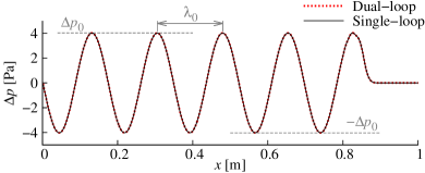
Figure 3: Pressure profiles of the acoustic waves at $t=2.5\times 10^{-3}\,\textup{s}$ using the single-loop and dual-loop solution procedures. The theoretical pressure amplitude $\Delta p_{0}=\pm\rho_{0}a_{0}\Delta u_{0}$ and wavelength $\lambda_{0}=a_{0}/f$ according to linear acoustic theory are given as a reference.

The execution time $\tau$ for the simulation of these acoustic waves using different linearisation and solution strategies are given in Table 1. The Newton linearisation of the transient terms of the momentum and energy equations yields a clear improvement in performance, with a speedup of factor $1.4$ to $1.5$ compared to the fixed-coefficient linearisation. Interestingly, while the simulations do not converge if the single-loop solution procedure is applied in conjunction with a fixed-coefficient linearisation of all terms, the single-loop solution procedure converges, and yields a shorter execution time than the dual-loop solution procedure, when the Newton linearisation is applied to the transient terms. The linearisation of the advection terms of the governing equations, however, does not have a significant impact on the execution times for the cases presented in Table 1. In fact, this is to be expected considering the small local changes in advecting velocity $\vartheta_{f}$ (i.e. the fluxes) and the low Mach number $M\approx 10^{-3}$, with the associated marginal changes in density $\rho$. Increasing the time-step $\Delta t$, the additional numerical stability associated with the $\vartheta$-Newton linearisation of the advection terms in the momentum and energy equations becomes apparent, see Table 2. If the fixed-coefficient linearisation is applied to the advection terms, the execution time of the simulation increases significantly as the Courant number exceeds unity and the solution algorithm fails to converge for $\textup{Co}=10$. However, applying the $\vartheta$-Newton linearisation, convergence is stable and rapid for all tested Courant numbers. Note that the amplitude and the wavelength of the acoustic waves are not predicted accurately for $\textup{Co}>1$, with the amplitude decaying and the wavelength increasing as the waves propagate downstream.

Table 1: Execution time $\tau$ for the propagation of the acoustic waves with different linearisation and solution strategies.

Case	Continuity	Momentum and energy		$\tau$ [s]
	Advection	Transient	Advection	Dual-loop	Single-loop
A	fixed-coeff.	fixed-coeff.	fixed-coeff.	$2529$	–
B	Newton	fixed-coeff.	fixed-coeff.	$2521$	–
C	fixed-coeff.	Newton	fixed-coeff.	$1668$	$1211$
D	Newton	Newton	fixed-coeff.	$1697$	$1192$
E	Newton	Newton	$\rho$-Newton	$1731$	$1231$
F	Newton	Newton	$\vartheta$-Newton	$1718$	$1254$
G	Newton	Newton	full-Newton	$1786$	$1211$

Table 2: Execution time $\tau$ for the propagation of the acoustic waves, simulated with different Courant numbers Co and different linearisation strategies applied to the advection terms of the momentum and energy equations, using the single-loop solution procedure. The Newton linearisation is applied to the advection term of the continuity equation and the transient terms of the momentum and energy equations.

Linearisation	$\tau$ [s]
	$\textup{Co}=0.5$	$\textup{Co}=1$	$\textup{Co}=2$	$\textup{Co}=10$
fixed-coeff.	$316$	$248$	$527$	–
$\vartheta$-Newton	$325$	$191$	$124$	$43$

In summary, in this low Mach number case, the Newton linearisation of the transient terms in the momentum and energy equations provides a significant speedup, whereas the linearisation of the advection terms does not have a sizeable impact on the performance of the numerical algorithm, since changes in fluxes and density are small. However, at large Courant numbers the $\vartheta$-Newton linearisation provides an improved stability and convergence of the solution algorithm.

5.2 Shock tube

Due to their conceptual simplicity and well-defined theoretical solution, shock tubes are frequently used test-cases for the validation and comparison of numerical methods. The considered shock tube, which was originally proposed by Sod [38], features a shock wave, a rarefaction fan and a contact discontinuity and, hence, provides a comprehensive test-case to analyse the performance and convergence behaviour of the considered linearisation and solution strategies.

The discontinuity of initial conditions separating the left state and the right state is initially located in the middle of the one-dimensional domain with a length of $1\,\textup{m}$, which is represented with $400$ equidistant cells. The initial conditions of the left and right states are [38]

$$\begin{array}[]{lllll}u_{\textup{L}}=0\,\textup{m}\,\textup{s}^{-1},&p_{\textup{L}}=1.0\,\textup{Pa},&\rho_{\textup{L}}=1.000\,\textup{kg}\,\textup{m}^{-3},\\ u_{\textup{R}}=0\,\textup{m}\,\textup{s}^{-1},&p_{\textup{R}}=0.1\,\textup{Pa},&\rho_{\textup{R}}=0.125\,\textup{kg}\,\textup{m}^{-3}.\end{array}$$

The applied time-steps $\Delta t$ correspond to $\textup{Co}=a_{\textup{L}}\Delta t/\Delta x\in\{0.1,0.5\}$ and the applied solution tolerance is $\eta=10^{-8}$. The simulations are conducted on a single core of an Intel Xeon processor with Haswell architecture. The results for all considered linearisation and solution strategies are in very good agreement with each other and the theoretical Riemann solution for both considered Courant numbers, as seen in Figs. 4 and 5.

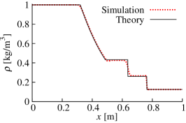
(a) Density $\rho$

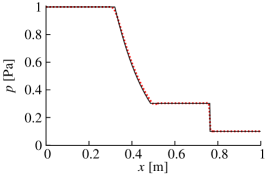
(b) Pressure $p$

Figure 4: Density and pressure profiles of the shock tube at $t=0.15\,\textup{s}$, obtained with $\textup{Co}=0.1$. The theoretical Riemann solution is shown as a reference.

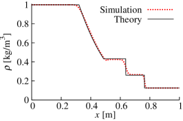
(a) Density $\rho$

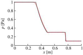
(b) Pressure $p$

Figure 5: Density and pressure profiles of the shock tube at $t=0.15\,\textup{s}$, obtained with $\textup{Co}=0.5$. The theoretical Riemann solution is shown as a reference.

The execution times $\tau$ for $\textup{Co}=0.1$, listed in Table 3, exhibit a similar pattern as observed for the propagation of acoustic waves in Section 5.1. Using the dual-loop solution procedure, the Newton linearisation of the transient terms of the momentum and energy equations provides an appreciable speedup. The Newton linearisation of the transient terms also yields converged solutions if the single-loop solution procedure is applied, resulting in further speedup. The Newton linearisation of the advection terms, on the other hand, has no significant impact on the performance of the solution algorithm. Increasing the Courant number to $\textup{Co}=0.5$, for which the execution times are also given in Table 3, the dual-loop solution procedure does not yield a converged result if all transient and advection terms are linearised with the fixed-coefficient linearisation, whereas the Newton linearisation of the advection term of the continuity equation exhibits a clear performance benefit. In addition, with the single-loop solution procedure, it is necessary to apply the $\vartheta$-Newton linearisation to the advection terms of the momentum and energy equations to yield a converged solution.

Table 3: Execution time $\tau$ for the shock tube with $\textup{Co}\in\{0.1,0.5\}$, using different linearisation and solution strategies.

Case	Continuity	Momentum and energy		$\tau$ [s] for $\textup{Co}=0.1$		$\tau$ [s] for $\textup{Co}=0.5$
	Advection	Transient	Advection	Dual-loop	Single-loop	Dual-loop	Single-loop
A	fixed-coeff.	fixed-coeff.	fixed-coeff.	$437$	–	–	–
B	Newton	fixed-coeff.	fixed-coeff.	$413$	–	$137$	–
C	fixed-coeff.	Newton	fixed-coeff.	$325$	$142$	$235$	–
D	Newton	Newton	fixed-coeff.	$315$	$144$	$111$	–
E	Newton	Newton	$\rho$-Newton	$299$	$137$	$111$	–
F	Newton	Newton	$\vartheta$-Newton	$317$	$150$	$103$	$49$
G	Newton	Newton	full-Newton	$299$	$152$	$98$	$41$

The convergence rates of the outer loop $q_{m}$ and the inner loop $q_{n}$ for the first and last time-steps of the simulations conducted with the dual-loop solution procedure and $\textup{Co}=0.1$ are shown in Figs. 6 and 7, respectively, for three different linearisation strategies. The outer loop converges with a similar and almost constant convergence rate of $q_{m}\approx 1.25$ in all three cases, as seen Fig. 6. However, large differences in the convergence behaviour can be observed in Fig. 7 for the inner loop. Case A, which corresponds to a fixed-coefficient linearisation for all nonlinear terms, exhibits strong oscillations of the convergence rate $q_{n}$, see Fig. 7a; in the first time-step $q_{n}$ even becomes negative after each outer loop. Applying a Newton linearisation to the transient terms of the momentum and energy equations (Case C), see Fig. 7b, reduces the amplitude of these oscillations of the convergence rate $q_{n}$ substantially, circumventing negative convergence rates. The convergence becomes even smoother when a Newton linearisation is applied to all nonlinear terms (Case G), with $q_{n}\approx 2.6$ in the first time-step and $q_{n}\approx 3.8$ in the last time-step, as seen in Fig. 7c. Examining the convergence obtained with the single-loop solution procedure, shown in Fig. 8, shows that the full-Newton linearisation of the advection terms of the momentum and energy equations (Case G) yields a smooth convergence behaviour, while applying only the $\rho$-Newton (Case E) or the $\vartheta$-Newton (Case F) linearisations yields oscillations of the convergence rate $q_{n}$. The convergence rate $q_{n}$ is nominally lower with the single-loop solution procedure than with the dual-loop procedure, which is attributed to the stronger nonlinearity of the governing equations, because density is dependent on both pressure and temperature simultaneously using the single-loop solution procedure.

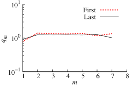
(a) Case A

(b) Case C

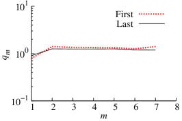
(c) Case G

Figure 6: Rate of convergence $q_{m}$, Eq. (36), for the shock tube, obtained with the dual-loop solution procedure and $\textup{Co}=0.1$, of the first and last time-steps for different linearisation strategies (see Table 3).

(a) Case A

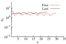
(b) Case C

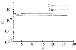
(c) Case G

Figure 7: Rate of convergence $q_{n}$, Eq. (35), for the shock tube, obtained with the dual-loop solution procedure and $\textup{Co}=0.1$, of the first and last time-steps for different linearisation strategies (see Table 3).

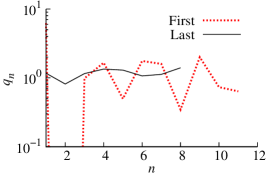
(a) Case D

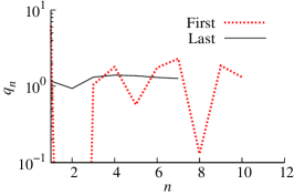
(b) Case E

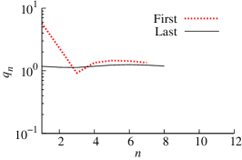
(c) Case F

Figure 8: Rate of convergence $q_{n}$, Eq. (35), for the shock tube, obtained with the single-loop solution procedure and $\textup{Co}=0.1$, of the first and last time-steps for different linearisation strategies (see Table 3).

5.3 Supersonic flow over a forward-facing step

The two-dimensional supersonic flow over a forward-facing step is frequently used to test new numerical methods and algorithms. Following Woodward and Colella [39], the computational domain is $3\,\textup{m}\times 1\,\textup{m}$ with a step of height $0.2\,\textup{m}$, positioned at $x=0.6\,\textup{m}$. The flow entering the domain has a Mach number of $M=u/a_{0}=3$. The mesh spacing of the applied equidistant Cartesian mesh is $\Delta x=0.01\,\textup{m}$, the applied time-steps $\Delta t$ correspond to $\textup{Co}=u\Delta t/\Delta x\in\{0.3,0.9\}$, and the applied solution tolerance is $\eta=10^{-7}$. The particular challenge of this test-case is the spatiotemporally evolving shock waves and the associated development of a transonic flow, as well as large pressure gradients. Figures 10 and 10 show the Mach number and pressure contours of the evolving transonic flow at $t=2\,\textup{s}$ and $t=4\,\textup{s}$, respectively, which are in good agreement with previously reported results [39, 40]. The simulations are conducted on a single compute node equipped with two Intel Xeon processors (Haswell architecture) containing $10$ cores each.

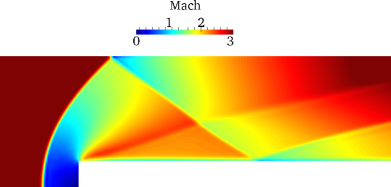
(a) Mach number $M$

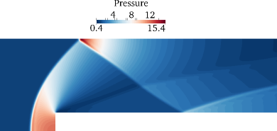
(b) Pressure $p$

Figure 9: Mach number and pressure contours of the supersonic flow over a forward-facing step at $t=2\,\textup{s}$, with $\textup{Co}=0.9$.

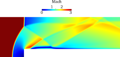
(a) Mach number $M$

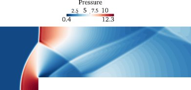
(b) Pressure $p$

Figure 10: Mach number and pressure contours of the supersonic flow over a forward-facing step at $t=4\,\textup{s}$, with $\textup{Co}=0.9$.

The execution times $\tau$ for $\textup{Co}=0.3$ are given in Table 4, using both the single- and dual-loop solution procedures. Note that applying a fixed-coefficient linearisation to the advection term of the continuity equation does not yield a converged solution for the considered Courant numbers with either of the applied solution procedures. In conjunction with the dual-loop solution procedure, the reduction in execution time as a result of applying the Newton linearisation to the transient terms of the momentum and energy equations, instead of the fixed-coefficient linearisation, is similar to the cases discussed in the previous sections. Although the linearisation of the advection terms has no substantial impact with respect to the solution time, the convergence rate $q_{n}$ of the inner loop is less oscillatory applying a Newton linearisation to the transient or advection terms, as seen in Fig. 11. If the time-step is increased to $\textup{Co}=0.9$, the $\rho$-Newton linearisation of the advection terms in the momentum and energy equations turns out to be crucial with respect to the performance and stability of the solution algorithm, as seen in Table 4. In fact, a converged result is obtained only with the $\rho$-Newton linearisation when the single-loop solution procedure is applied. The fully implicit treatment of density, through the Newton linearisation of the transient terms together with the $\rho$-Newton linearisation of the advection terms, provides a strong implicit pressure-density coupling, which is particularly significant in the transonic flow regime. Nevertheless, applying the full-Newton linearisation by adding the $\vartheta$-Newton linearisation further improves the convergence behaviour and circumvents negative convergence rates, as seen in Fig. 12, albeit with only a small reduction of the execution time.

Table 4: Execution time $\tau$ for the flow over a forward-facing step with $\textup{Co}\in\{0.3,0.9\}$, using different linearisation and solution strategies.

Case	Continuity	Momentum and energy		$\tau\,[\textup{s}]$ for $\textup{Co}=0.3$		$\tau\,[\textup{s}]$ for $\textup{Co}=0.9$
	Advection	Transient	Advection	Dual-loop	Single-loop	Dual-loop	Single-loop
B	Newton	fixed-coeff.	fixed-coeff.	$4966$	–	$5846$	–
D	Newton	Newton	fixed-coeff.	$2689$	$1818$	$2886$	–
E	Newton	Newton	$\rho$-Newton	$2763$	$1841$	$1769$	$1035$
F	Newton	Newton	$\vartheta$-Newton	$2967$	$1925$	$3079$	–
G	Newton	Newton	full-Newton	$2860$	$1940$	$1711$	$921$

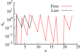
(a) Case B

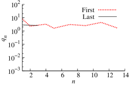
(b) Case D

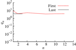
(c) Case G

Figure 11: Rate of convergence $q_{n}$, Eq. (35), for the flow over a forward-facing step, obtained with the dual-loop solution procedure and $\textup{Co}=0.3$, of the first and last time-steps for different linearisation strategies (see Table 4).

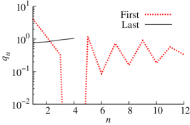
(a) Case E

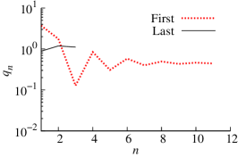
(b) Case G

Figure 12: Rate of convergence $q_{n}$, Eq. (35), for the flow over a forward-facing step, obtained with the single-loop solution procedure and $\textup{Co}=0.9$, of the first and last time-steps for different linearisation strategies (see Table 4).

5.4 Supersonic flow over a cone

As a final test-case, the three-dimensional supersonic flow over a circular cone is simulated. The cone, schematically shown in Fig. 13a, has a radius of $r=0.05\,\textup{m}$, a length of $l=0.1\,\textup{m}$ and the cone angle is $\beta=10^{\circ}$. The flow with $M=2$ is oriented with an angle of attack of $\psi=10^{\circ}$ to the primary axis of the cone. Because of the symmetry of the flow, only half of the cone is simulated, in a computational domain represented by a tetrahedral mesh with approximately $7.41\times 10^{5}$ cells, shown in Fig. 13b together with the Mach number contours at steady state. The applied time-step corresponds to $\textup{Co}=0.54$ and the solution tolerance is $\eta=10^{-7}$. Following Xiao et al. [24], the domain is initialised with uniform pressure $p_{0}=10^{5}\,\textup{Pa}$, temperature $T_{0}=300\,\textup{K}$ and velocity $u_{0}=695.59\,\textup{m}\,\textup{s}^{-1}$, corresponding to $M=2$. Xiao et al. [24] compared the results obtained with the applied numerical framework for supersonic flows over different circular cones favourably against previous studies [41, 42]. The presented simulations are stopped at $t=7.5\times 10^{-5}\,\textup{s}$, at which point the flow has assumed a steady state. The simulations are conducted on a single compute node equipped with two Intel Xeon processors (Haswell architecture) containing $10$ cores each.

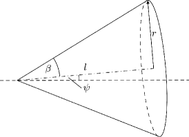
(a) Schematic illustration

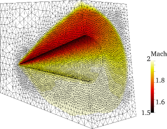
(b) Mach number contours with computational mesh

Figure 13: Schematic illustration of the circular cone with radius $r$, length $l$, cone angle $\beta$ and angle of attack $\psi$ and steady-state Mach number contours with the applied computational mesh of the flow with $M=2$ over the considered circular cone ($r=0.05\,\textup{m}$, $l=0.1\,\textup{m}$, $\beta=10^{\circ}$, $\psi=10^{\circ}$).

The execution times $\tau$ of the simulation with both the single- and dual-loop solution procedures are given in Table 5. Similar to the flow over the forward-facing step in Section 5.3, simulations without Newton linearisation of the advection term of the continuity equation do not yield a converged solution for the considered Courant number. In addition, even for the dual-loop solution procedure, a Newton linearisation of the transient terms of the momentum and energy equations is required for convergence. The $\rho$-Newton linearisation of the advection terms in the momentum and energy equations is found to be critical for the performance and stability of the solution algorithm, as similarly observed in Section 5.3, in particular using the single-loop solution procedure. The difference in execution time between the dual-loop and the single-loop solution procedures is noticeably smaller than in all other considered cases, which may be attributed to the strong coupling of pressure and density in the supersonic regime. In particular, with the Newton linearisation of the transient terms and the $\rho$-Newton linearisation of the advection terms, pressure and density are coupled implicitly in both the single-loop and the dual-loop solution procedures; the implicit coupling of the equation system, thus, closely represents the nature of the flow. At the same time, the influence of changes of the fluxes, i.e. the advecting velocity $\vartheta_{f}$, are less significant in the supersonic regime, which explains the small impact of the $\vartheta$-Newton linearisation of the advection terms. This can also be observed in Fig. 14, which shows the residual norms obtained with both solution procedures; a clear difference in convergence behaviour can be seen between cases with and without $\rho$-Newton linearisation, whereas the $\vartheta$-Newton linearisation has an almost negligible influence on the convergence.

Table 5: Execution time $\tau$ for the supersonic flow over a cone with $M=2$ and $\textup{Co}=0.54$, using different linearisation and solution strategies.

Case	Continuity	Momentum and energy		$\tau\,[\textup{s}]$
	Advection	Transient	Advection	Dual-loop	Single-loop
B	Newton	fixed-coeff.	fixed-coeff.	–	–
D	Newton	Newton	fixed-coeff.	$19517$	–
E	Newton	Newton	$\rho$-Newton	$12117$	$10616$
F	Newton	Newton	$\vartheta$-Newton	$17130$	–
G	Newton	Newton	full-Newton	$12137$	$10485$

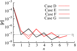
(a) Dual-loop solution procedure

(b) Single-loop solution procedure

Figure 14: $L_{2}$-norm of the residual vector $\boldsymbol{r}$, Eq. (33), of the first-time step for the supersonic flow over a circular cone, using a) the dual-loop solution procedure and b) the single-loop solution procedure, with different linearisation strategies. Black (red) lines are used for cases with (without) $\rho$-Newton linearisation of the advection terms. Note that for the shown cases using the dual-loop solution procedure, every maximum in $\|\boldsymbol{r}\|$ is associated with an increment of the outer loop, $m\leftarrow m+1$, see Fig. 2b, i.e. it follows a density update based on pressure $p$ and the updated temperature $T$.

6 Conclusions

Different linearisation and iterative solution strategies have been analysed and compared in the context of a fully-coupled pressure-based algorithm for compressible flows at all speeds, with the aim of elucidating their impact on performance and stability of the algorithm. To this end, the analysis has focused on test-cases with compression and expansion waves in all Mach number regimes. The presented results highlight a substantial influence of the chosen linearisation and provide new insight into the design of efficient and robust pressure-based algorithms for compressible flows. The discussed single-loop and dual-loop solution algorithms do not feature underrelaxation procedures or other tuning parameters, and are, therefore, straightforward in their application; although the reduction of nonlinearity through a barotropic density update in the inner loop of the dual-loop solution procedure is perhaps somewhat akin to an underrelaxation.

The strong implicit coupling of pressure, density and velocity through a Newton linearisation of the transient terms of the momentum and energy equations was found to be the primary performance driver in all Mach number regimes, providing a speedup of up to factor $2.2$ for the considered test-cases. The linearisation of the transient term was further observed to be a prerequisite for the application of the single-loop solution procedure, resulting in a further reduction of the execution time for flows in all Mach number regimes. The reason for this improved performance and stability is attributed to the smoother and less oscillatory convergence behaviour of the iterative solution algorithm, in particular with respect to the nonlinear residual. Even though, applying the dual-loop solution procedure, the peak convergence rates of the inner loop are similarly high for the considered test-cases, the convergence rate quickly drops below $1$ without the Newton linearisation of the transient terms.

The Newton linearisation of the advection terms of the continuity, momentum and energy equations was found to have a negligible influence on the performance and stability at low Mach numbers, in conjunction with low Courant numbers. In fact, due to the increase in the number of non-zero coefficients of the sparse coefficient matrix of the linear system of governing equations, the $\vartheta$-Newton linearisation of the advection terms was found to slightly increase the execution time for low Mach number flows, e.g. the propagation of acoustic waves. However, the Newton linearisation of the advection term of the continuity equation becomes essential for the stability of the solution algorithm for high Mach number flows. With regards to the linearisation of the advection terms of the momentum and energy equations, the $\rho$-Newton linearisation was also found to be important for the performance and stability for flows with large Mach numbers. The $\vartheta$-Newton linearisation of the advection terms improves the convergence and stability for flows in all Mach number regimes when the Courant number is large, with both the single-loop and dual-loop solution procedures. In fact, the only linearisation strategy that yields a stable convergence for all considered test-cases, irrespective of the considered Mach number, Courant number and solution strategy, is the full-Newton linearisation of all advection terms in conjunction with the Newton linearisation of the transient terms.

The dual-loop solution procedure has been shown to be, in general, more stable than the single-loop solution procedure, owing to the reduction in nonlinearity through the barotropic density update in the inner loop. This surplus in stability comes at the cost of longer execution times. Hence, when the single-loop solution procedure converges, it yields a significant reduction in execution time; for the considered shock-tube, for instance, switching from the dual-loop to the single-loop solution procedure reduces the execution time by factor $2.3$.

In summary, the presented study highlights the importance of a careful linearisation of the governing nonlinear equations for compressible flows. To this end, a full Newton linearisation of all transient and advection terms of the governing equations is found to be overall beneficial, improving the performance and stability of the solution algorithm, and fully exploits the implicit coupling via the simultaneous solution of the governing equations in the applied fully-coupled pressure-based algorithm. The accelerated convergence and improved stability of the solution algorithm, in conjunction with the elimination of all underrelaxation measures and increase in the applied Courant number, has been shown to speedup the simulations by several times compared to a simple but widely applied fixed-coefficient linearisation, for flows in all Mach number regimes.

References

- Tannehill et al. [1997] J. Tannehill, R. Pletcher, D. Anderson, Computational Fluid Mechanics and Heat Transfer, Taylor & Francis, second edition, 1997.
- Wesseling [2001] P. Wesseling, Principles of Computational Fluid Dynamics, Springer, 2001.
- Beam and Warming [1978] R. M. Beam, R. F. Warming, An Implicit Factored Scheme for the Compressible Navier-Stokes Equations, AIAA Journal 16 (1978) 393–402.
- MacCormack [1982] R. W. MacCormack, A Numerical Method for Solving the Equations of Compressible Viscous Flow, AIAA Journal 20 (1982) 1275–1281.
- Turkel et al. [1997] E. Turkel, R. Radespiel, N. Kroll, Assessment of preconditioning methods for multidimensional aerodynamics, Computers & Fluids 26 (1997) 613–634.
- van der Heul et al. [2003] D. van der Heul, C. Vuik, P. Wesseling, A conservative pressure-correction method for flow at all speeds, Computers & Fluids 32 (2003) 1113–1132.
- Cordier et al. [2012] F. Cordier, P. Degond, A. Kumbaro, An Asymptotic-Preserving all-speed scheme for the Euler and Navier–Stokes equations, Journal of Computational Physics 231 (2012) 5685–5704.
- Miettinen and Siikonen [2015] A. Miettinen, T. Siikonen, Application of pressure- and density-based methods for different flow speeds: Application of pressure- and density-based methods for different flow speeds, International Journal for Numerical Methods in Fluids 79 (2015) 243–267.
- Harlow and Amsden [1971] F. H. Harlow, A. A. Amsden, A numerical fluid dynamics calculation method for all flow speeds, Journal of Computational Physics 8 (1971) 197–213.
- Van Doormaal et al. [1987] J. Van Doormaal, G. Raithby, B. McDonald, The Segregated Approach to Predicting Viscous Compressible Fluid Flows, ASME Journal of Turbomachinery 109 (1987) 268–277.
- Chen and Pletcher [1991] K.-H. Chen, R. Pletcher, Primitive Variable, Strongly Implicit Calculation Procedure for Viscous Flows at All Speeds, AIAA Journal 29 (1991) 1241–1249.
- Acharya et al. [2007] S. Acharya, B. R. Baliga, K. Karki, J. Y. Murthy, C. Prakash, S. P. Vanka, Pressure-Based Finite-Volume Methods in Computational Fluid Dynamics, Journal of Heat Transfer 129 (2007) 407.
- Moukalled et al. [2016] F. Moukalled, L. Mangani, M. Darwish, The Finite Volume Method in Computational Fluid Dynamics: An Advanced Introduction with OpenFOAM and Matlab, Springer, 2016.
- Harlow and Amsden [1968] F. H. Harlow, A. A. Amsden, Numerical calculation of almost incompressible flow, Journal of Computational Physics 3 (1968) 80–93.
- Issa et al. [1986] R. Issa, A. Gosman, A. Watkins, The computation of compressible and incompressible recirculating flows by a non-iterative implicit scheme, Journal of Computational Physics 62 (1986) 66–82.
- Karki and Patankar [1989] K. C. Karki, S. V. Patankar, Pressure based calculation procedure for viscous flows at all speeds in arbitrary configurations, AIAA Journal 27 (1989) 1167–1174.
- Issa and Javareshkian [1998] R. I. Issa, M. H. Javareshkian, Pressure-Based Compressible Calculation Method Utilizing Total Variation Diminishing Schemes, AIAA Journal 36 (1998) 1652–1657.
- Moukalled and Darwish [2000] F. Moukalled, M. Darwish, A unified formulation of the segregated class of algorithms for fluid flow at all speeds, Numerical heat transfer, Part B. 37 (2000) 103–139.
- Demirďzić et al. [1993] I. Demirďzić, v. Lilek, M. Perić, A collocated finite volume method for predicting flows at all speeds, International Journal for Numerical Methods in Fluids 16 (1993) 1029–1050.
- Karimian and Schneider [1994] S. M. H. Karimian, G. E. Schneider, Pressure-based computational method for compressible and incompressible flows, Journal of Thermophysics and Heat Transfer 8 (1994) 267–274.
- Karimian and Schneider [1995] S. M. H. Karimian, G. E. Schneider, Pressure-based control-volume finite element method for flow at all speeds, AIAA Journal 33 (1995) 1611–1618.
- Chen and Przekwas [2010] Z. Chen, A. J. Przekwas, A coupled pressure-based computational method for incompressible/compressible flows, Journal of Computational Physics 229 (2010) 9150–9165.
- Darwish and Moukalled [2014] M. Darwish, F. Moukalled, A fully coupled navier-stokes solver for fluid flow at all speeds, Numerical Heat Transfer, Part B: Fundamentals 65 (2014) 410–444.
- Xiao et al. [2017] C.-N. Xiao, F. Denner, B. van Wachem, Fully-coupled pressure-based finite-volume framework for the simulation of fluid flows at all speeds in complex geometries, Journal of Computational Physics 346 (2017) 91–130.
- Kunz et al. [1999] R. Kunz, W. Cope, S. Venkateswaran, Development of an implicit method for multi-fluid flow simulations, Journal of Computational Physics 152 (1999) 78–101.
- Dennis and Schnabel [1996] J. E. Dennis, R. B. Schnabel, Numerical Methods for Unconstrained Optimization and Nonlinear Equations, Society for Industrial and Applied Mathematics, 1996.
- Darbandi et al. [2008] M. Darbandi, E. Roohi, V. Mokarizadeh, Conceptual linearization of Euler governing equations to solve high speed compressible flow using a pressure-based method, Numerical Methods for Partial Differential Equations 24 (2008) 583–604.
- Darbandi and Mokarizadeh [2004] M. Darbandi, V. Mokarizadeh, A modified pressure-based algorithm to solve flow fields with shock and expansion waves, Numerical Heat Transfer, Part B: Fundamentals 46 (2004) 497–504.
- Ferziger and Perić [2002] J. Ferziger, M. Perić, Computational Methods for Fluid Dynamics, Springer Verlag, Berlin Heidelberg New York, 3. edition, 2002.
- Roe [1986] P. Roe, Characteristic-based schemes for the euler equations, Annual Review of Fluid Mechanics 18 (1986) 337–365.
- Denner et al. [2018] F. Denner, C.-N. Xiao, B. van Wachem, Pressure-based algorithm for compressible interfacial flows with acoustically-conservative interface discretisation, Journal of Computational Physics 367 (2018) 192–234.
- Demirďzić and Muzaferija [1995] I. Demirďzić, S. Muzaferija, Numerical method for coupled fluid flow, heat transfer and stress analysis using unstructured moving meshes with cells of arbitrary topology, Computer Methods in Applied Mechanics and Engineering 125 (1995) 235–255.
- Balay et al. [1997] S. Balay, W. Gropp, L. C. McInnes, B. F. Smith, Efficient Management of Parallelism in Object Oriented Numerical Software Libraries, in: E. Arge, A. Bruasat, H. Langtangen (Eds.), Modern Software Tools in Scientific Computing, Birkhaeuser Press, 1997, pp. 163–202.
- Balay et al. [2017a] S. Balay, S. Abhyankar, M. F. Adams, J. Brown, P. Brune, K. Buschelman, L. Dalcin, V. Eijkhout, W. D. Gropp, D. Kaushik, M. G. Knepley, L. C. McInnes, K. Rupp, B. F. Smith, S. Zampini, H. Zhang, H. Zhang, PETSc Web page, http://www.mcs.anl.gov/petsc, 2017a.
- Balay et al. [2017b] S. Balay, S. Abhyankar, M. F. Adams, J. Brown, P. Brune, K. Buschelman, L. Dalcin, V. Eijkhout, D. Kaushik, M. G. Knepley, D. A. May, L. C. McInnes, W. D. Gropp, K. Rupp, P. Sanan, B. F. Smith, S. Zampini, H. Zhang, H. Zhang, PETSc Users Manual, Technical Report ANL-95/11 - Revision 3.8, Argonne National Laboratory, 2017b.
- Dembo et al. [1982] R. Dembo, S. Eisenstat, T. Steihaug, Inexact newton methods, SIAM Journal on Numerical Analysis 19 (1982) 400–408.
- Anderson [2003] J. D. Anderson, Modern Compressible Flow: With a Historical Perspective, McGraw-Hill New York, 2003.
- Sod [1978] G. A. Sod, A survey of several finite difference methods for systems of nonlinear hyperbolic conservation laws, Journal of Computational Physics 27 (1978) 1–31.
- Woodward and Colella [1984] P. Woodward, P. Colella, The Numerical Simulation of Two-Dimensional Fluid Flow with Strong Shocks, Journal of Computational Physics 173 (1984) 115–173.
- Jasak [1996] H. Jasak, Error Analysis and Estimation for the Finite Volume Method with Applications to Fluid Flow, Ph.D. thesis, Imperial College London, 1996.
- Sims [1964] J. Sims, Tables for Supersonic Flow around Right Circular Cones at Zero Angle of Attack, Technical Report NASA-SP-3004, NASA Marshall Space Flight Center, Huntsville, AL, USA, 1964.
- Kutler and Lomax [1971] P. Kutler, H. Lomax, A systematic development of the supersonic flow fields over and behind wings and wing-body configurations using a shock-capturing finite-difference approach, AIAA 9th Aerospace Science Meeting, AIAA Paper No. 71-99, 1971.