Effective tunnel conductance and effective ac conductivity of randomly strained graphene

Abstract

We consider a single-layer graphene with high ripples, so that the pseudo-magnetic fields due to these ripples are strong. If the magnetic length corresponding to a typical pseudo-magnetic field is smaller than the ripple size, the resulting Landau levels are local. Then the effective properties of the macroscopic sample can be calculated by averaging the local properties over the distribution of ripples. We find that this averaging does not wash out the Landau quantization completely. Average density of states (DOS) contains a feature (inflection point) at energy corresponding to the first Landau level in a typical field. Moreover, the frequency dependence of the ac conductivity contains a maximum at a frequency corresponding to the first Landau level in a typical field. This nontrivial behavior of the effective characteristics of randomly strained graphene is a consequence of non-equidistance of the Landau levels in the Dirac spectrum.

I Introduction

It is known that graphene deposited on different substrates, such as SiO₂, exhibits ripples.deposition1 These ripples essentially follow the corrugation of the substrate.

Already in the early days of the research on graphene it was predicteddeposition2 ; deposition2' (for review see Refs. deposition3, ; Maria1, ) that random strain, caused by ripples, can play the role of random magnetic field affecting the orbital motion of electrons and having opposite signs in different valleys.

Later, a direct evidence of the substrate-induced ripples was reported in Refs. HeinzSTMimage, ; FuhrerTopography1, ; TopographySiO2, ; FuhrerTopographySi02, ; Zhitenev, , where the topography of the surface was revealed via the STM (scanning tunneling microscopy) images. The fact that the ripples indeed give rise to the pseudo-magnetic fields was directly confirmed in the experiments Refs. BerkleyBubble, ; MosesChan, ; AnotherTunneling, . In Refs. BerkleyBubble, ; MosesChan, ; AnotherTunneling, the staircases of the Landau levels were observed in the bias dependence of the local tunnel conductance. Another physical manifestation of the curvature-induced magnetic field is the sensitivity of transport to the external magnetic field applied parallel to the surface. This sensitivity was demonstrated experimentally in Refs. Folk1, ; Folk2, . Due to strain, a parallel magnetic field generates a pseudo-magnetic field normal to the surface which causes the electron dephasing.Maria ; Lewenkopf ; Lewenkopf1 Alternative explanationBaranger is common for electron motion along the rough interface: in course of this motion electron trajectory can enclose a finite flux even if the field is parallel to the graphene sheet on average.

The motivation for the current studies of the strained grapheneExperiment ; Andrei is a promise to manipulate the electron spectrum by tailoring the strain.Experiment1 For a review on “strain engineering” see Ref. FengLiuReview, .

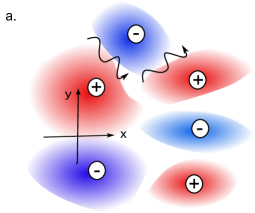
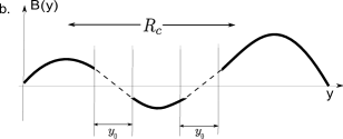
Figure 1: (Color online) (a) Schematic illustration of random pseudo-magnetic field induced by strain. In the red and blue regions the field has opposite signs. Typical size, $R_{c}$, of the regions is assumed to be much bigger than the typical magnetic length. Low-energy states originate from the white regions where magnetic field passes through zero. For these “snake”-like states electron propagates along the boundary $B=0$ and decays into both red and blue regions. (b) Since the extension, $y_{0}$, of the electron wave-function in the $y$-direction, which is normal to the direction of propagation, is much smaller than $R_{c}$, the magnetic field within $y_{0}$ can be linearized.

In the present paper we address one peculiar property of graphene with pseudo-magnetic fields. These fields create position-dependent staircases of Landau levels. Randomness in the “steps” of these staircases tends to smear the average density of states (DOS). It is not obvious whether or not this smearing is complete. Specifics of graphene with linear dispersion spectrum is that Landau levels are not equidistant in a constant magnetic field. We demonstrate that, as a consequence of this non-equidistance, the average DOS retains the memory about the Landau quantization.

If the random field changes smoothly along the plane, local Landau levels are formed in the strained regions. They manifest themselves in the local tunnel conductance.BerkleyBubble ; MosesChan We demonstrate that the average (over the surface area) tunnel conductance, $G$, still contains a feature reflecting the first Landau level in a typical field. Naturally, this feature is more pronounced in the derivative, $\frac{dG}{dV}$, of the conductance with respect to the bias voltage, $V$. This derivative saturates at high bias. Together with the average tunnel conductance, we calculate the average frequency-dependent ac conductivity, $\sigma(\Omega)$. It appears that a feature at $\Omega$ corresponding to the first Landau level in a typical field not only survives the averaging, but manifests itself stronger than in the tunnel conductance.

The bigger is the correlation length, $R_{c}$, of the random magnetic field, see Fig. 1, the more pronounced is the Landau quantization in the average DOS, or, in other words, the stronger is the depletion of the DOS near zero energy. Finite $R_{c}$ smears the quantization due to the emergence of the low-energy states. These states, which we study in the present paper, originate from the spatial regions where the random magnetic field passes through zero, as illustrated in Fig. 1.

II Average DOS

If the magnetic field does not change in space, then the DOS is given by

$$\rho(E,B)=\frac{1}{2\pi\ell_{B}^{2}}\sum_{n=-\infty}^{\infty}\delta\left(E-E_{n}\right),$$ (1)

where the energies, $E_{n}$, are the Landau levels in graphene

$$E_{n}={\text{s}gn}(n)\left(2e\hbar v_{F}^{2}|n|B\right)^{1/2}.$$ (2)

Here $v_{F}\approx 10^{6}$m/s is the Fermi velocity, and

$$\ell_{B}=\left(\frac{\hbar}{eB}\right)^{1/2}$$ (3)

is the magnetic length.

Actual shape, $\langle\rho(E,B)\rangle$, of the average DOS depends on the relation between the correlation radius, $R_{c}$, of the random field and the magnetic length, $\ell_{B}$, in the characteristic field, $B_{0}$. For $R_{c}\gg\ell_{B}$ adiabatic description applies. Within this description, the local DOS is given by Eq. (1) at every point, with $E_{n}$ being the levels in the field, $B$, at this point. Then $\langle\rho(E)\rangle$ is obtained by averaging of Eq. (1) over the distribution of $B$, i.e.

$$\langle\rho(E)\rangle=\frac{1}{B_{0}}\int\limits_{-\infty}^{\infty}dB\rho(E,B)F\Big{(}\frac{B}{B_{0}}\Big{)},$$ (4)

where the distribution function, $F$, is normalized, so that $\int_{-\infty}^{\infty}dxF(x)=1$.

The integration in Eq. (4) is performed with the help of the $\delta$-functions. Prior to the averaging, it is convenient to rewrite the DOS Eq. (1) in the form

$$\rho(E,B)=\frac{e|B|}{2\pi\hbar}\delta(E)+\frac{|E|}{\hbar^{2}v_{F}^{2}}\sum_{n=1}^{\infty}\frac{|B|}{n}\delta\left(|B|-\frac{E^{2}}{2\pi e\hbar v_{F}^{2}n}\right).$$ (5)

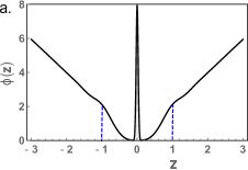
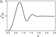
Figure 2: (Color online) (a) Average DOS in randomly strained graphene is plotted from Eq. (5) versus the dimensionless energy $z=E/w$, where $w$ is the Landau quantization energy in a typical pseudo-magnetic field. For demonstration purpose the $\delta$-peak at $E=0$ is broadened into a gaussian with a width $0.04$. Note that the first Landau level in a typical field survives the averaging and manifests itself as a feature near $z=1$. To elucidate this feature the derivative of average DOS is plotted in (b). It reveals not only the first but also the second Landau level.

Obviously, the $n=0$ Landau level is not smeared by averaging. However, the magnitude of the $\delta(E)$-term contains the magnetic field via $\ell_{B}$ and, thus, should be averaged. Equally, in $n\neq 0$ terms, the values of $B$ at which the arguments of the $\delta$-functions turn to zero, should be substituted into the prefactor $\frac{1}{\ell_{B}^{2}}$.

It follows from Eq. (4) that the characteristic scale of change of the average DOS is related to $B_{0}$ as

$$w=\Bigg{(}\frac{2ev_{\scriptscriptstyle F}^{2}B_{0}}{\hbar}\Bigg{)}^{1/2},$$ (6)

so that $\langle\rho(E)\rangle$ is a function of the dimensionless ratio

$$z=\frac{E}{w}.$$ (7)

We cast the result of averaging into the form

$$\langle\rho(E)\rangle=\frac{1}{2\pi\ell_{B_{0}}^{2}w}\phi\left(\frac{E}{w}\right).$$ (8)

where the dimensionless function $\phi(z)$ is given by

$$\phi(z)=2\overline{F}\delta(z)+4|z|^{3}\sum_{n=1}^{\infty}\frac{1}{n^{2}}F\Big{(}\frac{z^{2}}{n}\Big{)},$$ (9)

where $\overline{F}=\int_{0}^{\infty}dzzF(z)$.

For Gaussian $F(x)=\frac{1}{\pi^{1/2}}\exp(-x^{2})$ we have ${\overline{F}}=\frac{1}{2\pi^{1/2}}$. The small-$z$ asymptote of $\phi(z)$ follows from Eq. (9) upon setting $F(z)=\frac{1}{\pi^{1/2}}$

$$\phi(z)|_{|z|\ll 1}\approx\frac{4|z|^{3}}{\pi^{1/2}}\sum_{n=1}^{\infty}\frac{1}{n^{2}}=\frac{2\pi^{3/2}}{3}|z|^{3}.$$ (10)

This behavior reflects the depletion of the average DOS at small energies due to the formation of the Landau levels. The large-$z$ asymptote, $\phi(z)\approx 2|z|$, is determined by the terms $n\sim z^{2}\gg 1$, when the summation can be replaced by integration. Naturally, it recovers the DOS in a zero field. Our main finding is that, at intermediate $z$, the function $\phi(z)$ exhibits a feature (inflection point) near $z=1$ as shown in Fig. 2a. Presence of this feature indicates that the first Landau level survives the averaging. The feature becomes even more pronounced in the derivative $\phi^{\prime}(z)$ plotted in Fig. 2b. Actually, as seen in Fig. 2b, the derivative $\phi^{\prime}(z)$ contains an additional feature which corresponds to the second Landau level, so that it also survives the averaging in some form.

III Average ac conductivity

A standard expression for the ac conductivity, $\sigma(\Omega)$, in a constant magnetic field, see e.g. Ref. Magnetooptic, , reads

$$\sigma(\Omega)=\frac{e^{2}v_{F}^{2}|eB|}{\Omega}\sum_{n=0}^{\infty}\delta\Big{(}|E_{n}|+|E_{n+1}|-\Omega\Big{)}\\ {\small\times}\Big{\{}\big{[}n_{F}(-|E_{n}|)-n_{F}(|E_{n+1}|)\big{]}+\big{[}n_{F}(-|E_{n+1}|)-n_{F}(|E_{n}|)\big{]}\Big{\}}.$$ (11)

Here $n_{F}(E)=\left[\exp(E/T)+1\right]^{-1}$ is the Fermi distribution. The first term in the square brackets describes the transitions from the occupied hole level $(n+1)$ to the empty electron level $n$, while the second term describes the transitions from the occupied hole level $n$ to the empty electron level $(n+1)$.

In the limit $\Omega\gg w$, Eq. (11) yields $\sigma=\frac{e^{2}}{4\hbar}$, which is a standard result. Averaging over the distribution of pseudo-magnetic fields in Eq. (11) is quite similar to the averaging of the DOS. The result is expressed through a dimensionless function, $\Upsilon({\tilde{z}})$, of the dimensionless frequency ${\tilde{z}}=\Omega/w$. This result reads

$$\sigma(\Omega)=\frac{e^{2}}{4\hbar}\Upsilon({\tilde{z}}).$$ (12)

The form of the function $\Upsilon({\tilde{z}})$ is the following

$$\Upsilon({\tilde{z}})=8{\tilde{z}}^{2}\sum_{n=0}^{\infty}\frac{f_{n}({\tilde{z}},T)}{\left(\sqrt{n}+\sqrt{n+1}\right)^{4}}F\Bigg{(}\frac{{\tilde{z}}^{2}}{\left(\sqrt{n}+\sqrt{n+1}\right)^{2}}\Bigg{)},$$ (13)

where the temperature factor, $f_{n}({\tilde{z}},T)$, is defined as

$$f_{n}({\tilde{z}},T)=\frac{\exp(\lambda_{T}{\tilde{z}})}{4\cosh\left(\frac{\lambda_{T}{\tilde{z}}\sqrt{n}}{\sqrt{n}+\sqrt{n+1}}\right)\cosh\left(\frac{\lambda_{T}{\tilde{z}}\sqrt{n+1}}{\sqrt{n}+\sqrt{n+1}}\right)},$$ (14)

with $\lambda_{T}=\frac{w}{2T}$.

Note that there is an important difference between Eqs. (9) and (13). Namely, the summation in $\Upsilon({\tilde{z}})$ includes the term $n=0$. Due to this term, a peak in the average ac conductivity is present even without taking derivative, as shown in Fig. 3. This peak corresponds to the virtual transitions $0\rightarrow 1$ and $-1\rightarrow 0$ in the Kubo formula. It is seen from Fig. 3 that the peak remains pronounced up to high temperatures.

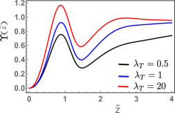
Figure 3: (Color online) The average ac conductivity is plotted from Eq. 13 versus the dimensionless frequency ${\tilde{z}}=\Omega/w$, where the characteristic frequency, $w$, is defined by Eq. (6). Unlike the DOS, the feature corresponding to the transition $0\rightarrow 1$ emerges even without taking the derivative. Black, blue, and red curves correspond to the temperatures $T=w$, $T=\frac{w}{2}$, and $T=\frac{w}{40}$, respectively.

IV Finite-$R_{c}$ correction

As it was mentioned above, the adiabatic description applies when the correlation length $R_{c}$ exceeds the magnetic length in a typical field. Even when this condition is met, there are low-energy states in a random magnetic field for which adiabatic description is inapplicable. These states originate from the regions where the random field passes through zero. As illustrated in Fig. 1a, the contours $B=0$ form a percolation network. As a result of the smallness of $B$, the corresponding local magnetic length is big and exceeds $R_{c}$. To establish the portion of these regions and their contribution to the DOS a full quantum mechanical description is required. The simplification which allows one to develop this description comes from the fact that the motion along the network $B=0$ has a one-dimensional character.Chalker1994

We start from the effective-mass Hamiltonian for an electron in the presence of an arbitrary magnetic field

$$\hat{H}=v_{F}\begin{pmatrix}0&&\hat{\pi}_{x}-i\hat{\pi}_{y}\\ \\ \hat{\pi}_{x}+i\hat{\pi}_{y}&&0\end{pmatrix},$$ (15)

where $\hat{\pi}={\bf\hat{k}}+\frac{e}{c}{\bf A}$, with ${\bf\hat{k}}$ being the momentum operator and ${\bf A}$ being the vector potential. The Hamiltonian Eq. (15) describes the states in a single valley.

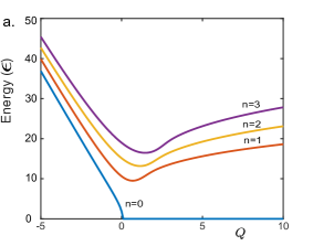
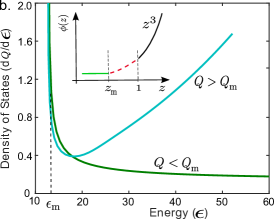
Figure 4: (Color online) (a) First four branches of the dispersion of the snake states obtained by the numerical solution of Eq. (20). (b) Two contributions to the dimensionless DOS, $\frac{dQ}{d\epsilon}$, are plotted from (a) for the branch $n=1$. Inset: schematic behavior of the dimensionless DOS plotted in Fig. 2 in the low-energy domain. The dependence $\phi(z)\propto z^{3}$ extends down to $z=z_{m}=\left(\frac{\ell_{B}}{R_{c}}\right)^{1/3}$ and is terminated as $z<z_{m}$, where the main contribution to the DOS comes from the snake states.

The crucial assumption, which will be justified later, is that, near the contour $B=0$, see Fig. 1a, the magnetic field can be linearized, see Fig. 1b, as $B=\frac{2B_{0}y}{R_{c}}$, so that the vector potential in the Landau gauge is given by ${\bf A}=(-\frac{B_{0}y^{2}}{R_{c}},0)$. This form of the vector potential allows the separation of variables in the Dirac equation, namely

$$\Psi=e^{ik_{x}x}\begin{pmatrix}\psi_{1}(y)\\ \\ \psi_{2}(y)\end{pmatrix},$$ (16)

where the components $\psi_{1}(y)$ and $\psi_{2}(y)$ satisfy the system of equations

$$\frac{E}{v_{F}}\psi_{1}=\left(k_{x}-\frac{eB_{0}y^{2}}{cR_{c}}\right)\psi_{2}+\frac{d\psi_{2}(y)}{dy},$$

$$\frac{E}{v_{F}}\psi_{2}=\left(k_{x}-\frac{eB_{0}y^{2}}{2R_{c}}\right)\psi_{1}-\frac{d\psi_{1}(y)}{dy}.$$ (17)

We can now introduce the dimensionless variables

$$y=y_{0}s,~{}~{}k_{x}=\frac{Q}{y_{0}},~{}~{}\epsilon=y_{0}\frac{E}{v_{F}},$$ (18)

where $y_{0}$ is given by

$$y_{0}=\left(\ell_{B}^{2}R_{c}\right)^{1/3},$$ (19)

and reduce the system Eq. (IV) to a single second-order differential equation for $\psi_{2}$

$$\frac{d^{2}\psi_{2}}{ds^{2}}+\Big{[}\left(Q-s^{2}\right)^{2}+2s\Big{]}\psi_{2}=\epsilon^{2}\psi_{2}.$$ (20)

This equation has the form of the Schrödinger equation with potential $U(s)=\left[\left(Q-s^{2}\right)^{2}+2s\right]$. Note that the term $2s$ in the potential is specific for the Dirac electron. For the Schrödinger electron in a magnetic fieldChalker1994 $B(y)\propto y$ this term is absent. It is this term which ensures that the level $\epsilon=0$ is robust.

From the expression Eq. (19) for $y_{0}$ we conclude that, by virtue of the condition $R_{c}\gg\ell_{B}$, the length $y_{0}$ lies in the interval

$$R_{c}\gg y_{0}\gg\ell_{B}.$$ (21)

First relation justifies linearizing of the magnetic field performed above. Second relation indicates that the energies of the snake states, described by the system Eq. (IV), are much smaller than the characteristic energy, $w$.

Consider a ripple of a size $\sim R_{c}$. Its area is $\sim R_{c}^{2}$. Snake states are confined along the perimeter, within a strip of a width $\sim y_{0}$, see Fig. 1. The area of the strip is $\sim y_{0}R_{c}$. Thus, for energies of the order of $w$, the relative correction, $\rho_{sn}(w)$, to the DOS due to finite $R_{c}$ is of the order of

$$\frac{\rho_{sn}(w)}{\langle\rho(w)\rangle}\sim\frac{y_{0}}{R_{c}}\sim\left(\frac{\ell_{B}}{R_{c}}\right)^{1/3}.$$ (22)

We now turn to the low-energy domain $E\ll w$, where the DOS is dominated by the snake states. The dispersion law, $\epsilon(Q)$, of the snake states, drifting along the contour $B=0$, can be found analytically in the limits of large negative and large positive $Q$. For negative $Q$, such that $|Q|\gg 1$, the potential can be replaced by $U(s)=Q^{2}+2|Q|s^{2}$. Then the Schrödinger equation Eq. (20) reduces to the harmonic oscillator equation yielding

$$\epsilon_{n}^{2}=Q^{2}+(2n+1)|2Q|^{1/2},~{}~{}~{}~{}~{}Q<0,~{}~{}|Q|\gg 1.$$ (23)

At large positive $Q$ the potential should be expanded near $s=Q^{1/2}$. Upon setting $s=\pm Q^{1/2}+s_{1}$, and assuming that $s_{1}\ll Q^{1/2}$, the potential takes the form $U(s)\approx 2Q^{1/2}+4Qs_{1}^{2}$, which is again the harmonic oscillator potential with frequency $2Q^{1/2}$. This leads to the following dispersion laws of the branches

$$\epsilon_{n}^{2}=4nQ^{1/2},~{}~{}~{}~{}~{}Q\gg 1.$$ (24)

Integer $n$ in Eqs. (23), (24) starts from $n=0$. Dispersion laws of the first four branches calculated numerically are shown in Fig. 4a. The asymptotes Eqs. (23), (24) are clearly seen in the plots. At large positive $Q$ the branches approach asymptotically the Landau levels in the bulk. The branch $n=0$ approaches $\epsilon=0$. However, with numerical accuracy, it merges with horizontal axis at $Q=0$. In Fig. 4b the dimensionless DOS, $\frac{dQ}{d\epsilon}$, is plotted for the branch $n=1$. This DOS contains two contributions from positive and from negative $Q$. It is seen that the first contribution dominates for dimensionless energies $\epsilon>\epsilon_{m}$, where $\epsilon_{m}$ is the minimal energy of the branch, see Fig. 4a.

To find the energy dependence of the DOS in the domain $\epsilon\gg 1$, we can use the asymptote (24) and cast it into the form

$$Q=\frac{\epsilon^{4}}{16n^{2}}.$$ (25)

In dimensional units Eq. (26) has the form

$$k_{x}=\frac{y_{0}^{3}E^{4}}{16n^{2}v_{F}^{4}}.$$ (26)

It is important that $\frac{dk_{x}}{dE}$ yields a one-dimensional DOS. To recalculate it into a real 2D DOS, we have to divide $\frac{dk_{x}}{dE}$ by $R_{c}$. This leads to the result

$$\rho_{sn}^{(n)}(E)=\frac{1}{R_{c}}\frac{dk_{x}}{dE}=\frac{y_{0}^{3}E^{3}}{4n^{2}R_{c}v_{F}^{4}}=\frac{\ell_{B}^{2}E^{3}}{4n^{2}v_{F}^{4}}.$$ (27)

Now it is easy to realize that, upon summation over $n$, Eq. (27) restores, within a factor, the behavior $\phi(z)\propto z^{3}$ derived above without accounting for the snake states. From this we conclude that the true behavior of $\phi(z)$ at small $z$ is the one shown schematically in the inset of Fig. 4b. Namely, the $z^{3}$-dependence extends down to minimal $z=z_{m}$ and saturates below $z=z_{m}$. The value of $z_{m}$ can be found from Eq. (18)

$$z_{m}=\frac{1}{w}\left(\frac{v_{F}}{y_{0}}\right)\sim\left(\frac{\ell_{B}}{R_{c}}\right)^{1/3}.$$ (28)

V Discussion

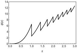
Figure 5: (Color online) Average DOS is plotted from Eq. (5) versus the dimensionless energy $z=E/E_{{\text{m}ax}}$ for the homogeneous distribution of pseudo-magnetic fields in the interval $\left(-B_{{\text{m}ax}},B_{{\text{m}ax}}\right)$. The energy $E_{{\text{m}ax}}$ is the Landau quantization energy in the field $B_{{\text{m}ax}}$. Multiple features originate from the sharp boundaries of the distribution. These boundaries are generic for the periodic arrangement of ripples.

(i) With regard to the observables, a pronounced peak in Fig. 2b should manifest itself in the derivative of the average differential conductance with respect to the bias voltage. In other words, not only the zero-bias peak, seen in differential conductanceBerkleyBubble , but also $n=\pm 1$ peaks survive the averaging over the ripples due to the substrate topography.

A peak in the average ac conductivity, $\sigma(\Omega)$, in Fig. 3 might manifest itself in the infrared characteristics of the rippled graphene sample. For example, for a typical field $1$T, the maximum in $\sigma(\Omega)$ corresponds to the frequency $\Omega=120$K and to the wavelength $100$$\mu m$. This frequency can be probed by photoconductivityGeim or by the measurement of the infrared transmission.Stormer In the latter case, the shape of transmission profile is determined by $\frac{d\sigma\left(\Omega\right)}{d\Omega}$.

(ii) From the STM images of graphene on different substrates,HeinzSTMimage ; FuhrerTopography1 ; TopographySiO2 ; FuhrerTopographySi02 ; Zhitenev it can be concluded that the realistic profile, $h(x,y)$, resembles a periodic structure. Such a quasi-periodicity implies that the distribution of $B({\bf r})$ has a sharp cutoff at some $B=B_{{\text{m}ax}}$. This is because $B({\bf r})$ is, essentially, the radius of curvature at the point ${\bf r}$.Maria ; Lewenkopf1 The consequence of this cutoff is a presence of numerous features in the average DOS corresponding to the Landau levels in the field $B=B_{{\text{m}ax}}$. To illustrate this point, we chose a homogeneous distribution of pseudo-magnetic fields which translates into $F(z)=\frac{1}{2}\theta(1-|z|)$. The resulting DOS calculated from Eq. (9) is shown in Fig. 5. We see that $\phi(z)$ exhibits a sawtooth structure as it approaches the bare DOS. More specifically, a microscopic treatmentMaria ; Lewenkopf1 of pseudo-magnetic fields induced by a bubble of concrete shape and with angular symmetry indicates that the maximum of pseudo-magnetic field corresponds to the points away from the center. Then the distribution, $F(B)$, diverges near $B_{{\text{m}ax}}$ as $(B_{{\text{m}ax}}-|B|)^{-1/2}$.

(iii) We emphasize that the inflection point in Fig. 2 is the consequence of Landau levels in the Dirac spectrum being non-equidistant. If they were equidistant, the function $\phi(z)$ would take the form $\phi(z)=z\sum_{n}\frac{1}{n^{2}}\exp\left(-\frac{z^{2}}{n^{2}}\right)$ instead of Eq. (9). Plotting this function indicates that the feature near $z=1$ is pronounced very weakly.

(iv) To explore the applicability of the adiabatic description we use the expressionExpressionForB for pseudo-vector potential in terms of the surface profile, $h(\bf r)$,

$$A_{x}({\bf r}) = \nu\frac{\Phi_{0}}{a}\Bigg{[}\left(\frac{\partial h}{\partial x}({\bf r})\right)^{2}-\left(\frac{\partial h}{\partial y}({\bf r})\right)^{2}\Bigg{]},$$

$$A_{y}({\bf r}) = -2\nu\frac{\Phi_{0}}{a}\Bigg{(}\frac{\partial h}{\partial x}({\bf r})\Bigg{)}\Bigg{(}\frac{\partial h}{\partial y}({\bf r})\Bigg{)},$$ (29)

where $\Phi_{0}=\frac{\hbar c}{e}$ is the flux quantum, and $a=1.42{\AA}$ is the lattice constant. Parameter $\nu\approx 0.6$ is expressed via the rate of change of the overlap intergralExpressionForB with $a$. From Eq. (V) we find the following general expression for the pseudo-magnetic field

$$B({\bf r})=2\nu\frac{\Phi_{0}}{a}\left[2\frac{\partial h}{\partial x}\frac{\partial^{2}h}{{\partial x}{\partial y}}-\frac{\partial h}{\partial y}\left(\frac{\partial^{2}h}{\partial y^{2}}-\frac{\partial^{2}h}{\partial x^{2}}\right)\right].$$ (30)

To calculate the average $\langle B^{2}({\bf r})\rangle$ it is convenient to switch in Eq. (30) to the Fourier transform, $h({\bm{r}})=\sum_{\bm{q}}h_{\bm{q}}\exp\left(i{\bm{q}}\cdot{\bm{r}}\right)$

$$B^{2}({\bf r})=4\nu^{2}\frac{\Phi_{0}^{2}}{a^{2}}|h_{\bm{q}}|^{2}|h_{\bm{Q}}|^{2}\\ \times\Big{[}4(q_{x}^{2}-q_{y}^{2})Q_{x}^{2}Q_{y}^{2}+4q_{x}q_{y}Q_{x}Q_{y}(Q_{x}^{2}-Q_{y}^{2})+q_{y}^{2}(Q_{x}^{2}+Q_{y}^{2})^{2}\Big{]}.$$ (31)

Only the last term contributes to $\langle B^{2}({\bf r})\rangle$. For the Gaussian correlator,

$$\langle h({\bf r}_{1})h({\bf r}_{2})\rangle=h_{0}^{2}\exp\left[-\frac{\left({\bf r}_{1}-{\bf r}_{2}\right)^{2}}{R_{c}^{2}}\right],$$ (32)

evaluation of Eq. (31) yields

$$\langle B^{2}({\bf r})\rangle=\left(\frac{16\nu\Phi_{0}h_{0}^{2}}{R_{c}^{3}a}\right)^{2}.$$ (33)

The latter expression can be rewritten in the form

$$\frac{\ell_{B}}{R_{c}}=\left(\frac{R_{c}a}{16\nu h_{0}^{2}}\right)^{1/2}.$$ (34)

For adiabatic description to apply the right-hand side should be small. It requires strong corrugation amplitude $h_{0}$, while, somewhat counterintuitively, the this corrugation cannot be too smooth for Landau levels to form within $R_{c}$. (the case opposite to Ref. OneBubbleNancySandler, ). Using the parameters $R_{c}=4$nm and $h_{0}=0.5$nm from Ref. BerkleyBubble, we get for the right-hand side the value $0.47$. Similar parameters $R_{c}=4\pm 2$nm and $h_{0}=0.6\pm 0.1$ were extracted in Ref. Folk2, from the transport measurements. Concerning the STM measurements, the parameters $R_{c}\approx 10$nm and $h_{0}\approx 0.5$nm reported in different papers HeinzSTMimage, ; FuhrerTopography1, ; TopographySiO2, ; FuhrerTopographySi02, are consistent with each other and correspond to the value $0.74$ in the right-hand side.

VI Acknowledgements

We are grateful to R. K. Morris who participated in this work at the early stage. The work was supported by the Department of Energy, Office of Basic Energy Sciences, Grant No. DE- FG02- 06ER46313.

References

- (1) S. V. Morozov, K. S. Novoselov, M. I. Katsnelson, F. Schedin, L. A. Ponomarenko, D. Jiang, and A. K. Geim, “Strong Suppression of Weak Localization in Graphene”, Phys. Rev. Lett. 97, 016801 (2006).
- (2) A. F. Morpurgo and F. Guinea, “Intervalley Scattering, Long-Range Disorder, and Effective Time-Reversal Symmetry Breaking in Graphene”, Phys. Rev. Lett. 97, 196804 (2006).
- (3) F. Guinea, M. I. Katsnelson, and A. H. Vozmediano, “ Midgap states and charge inhomogeneities in corrugated graphene”, Phys. Rev. B 77, 075422 (2008).
- (4) A. H. Castro Neto, F. Guinea, N. M. R. Peres, K. S. Novoselov, and A. K. Geim, “The electronic properties of graphene”, Rev. Mod. Phys. 81, 109 (2009).
- (5) M. A. H. Vozmediano, M. I. Katsnelson, and F. Guinea, “Gauge fields in graphene”, Phys. Rep. 496, 109 (2010).
- (6) E. Stolyarova, K. T. Rim, S. Ryu, J. Maultzsch, P. Kim, L. E. Brus, T. F. Heinz, M. S. Hybertsen, and G. W. Flynn, “High-resolution scanning tunneling microscopy imaging of mesoscopic graphene sheets on an insulating surface”, Proc. Natl. Acad. Sci. U.S.A. 104, 9209 (2007).
- (7) M. Ishigami, J. H. Chen, W. G. Cullen, M. S. Fuhrer, and E. D. Williams, “Atomic Structure of Graphene on SiO2”, Nano Lett. 7, 1643 (2007).
- (8) V. Geringer, M. Liebmann, T. Echtermeyer, S. Runte, M. Schmidt, R. Rückamp, M. C. Lemme, and M. Morgenstern, “Intrinsic and extrinsic corrugation of monolayer graphene deposited on SiO2”, Phys. Rev. Lett. 102, 076102 (2009).
- (9) W. G. Cullen, M. Yamamoto, K. M. Burson, J. H. Chen, C. Jang, L. Li, M. S. Fuhrer, and E. D. Williams, “High-fidelity conformation of graphene to SiO2 topographic features”, Phys. Rev. Lett. 105, 215504 (2010).
- (10) N. N. Klimov, S. Jung, S. Zhu, T. Li, C. A. Wright, S. D. Solares, D. B. Newell, N. B. Zhitenev, and J. A. Stroscio, “Electromechanical Properties of Graphene Drumheads”, Science 336, 1557 (2012).
- (11) N. Levy, S. A. Burke, K. L. Meaker, M. Panlasigui, A. Zettl, F. Guinea, A. H. Castro Neto, and M. F. Crommie, “Strain-Induced Pseudo Magnetic Fields Greater Than 300 Tesla in Graphene Nanobubbles”, Science 329, 1191700 (2010).
- (12) H. Yan, Y. Sun, L. He, J.-C. Nie, and M. H. W. Chan, “Observation of Landau-level-like quantization at 77 K along a strained-induced graphene ridge”, Phys. Rev. B 85, 035422 (2012).
- (13) S.-Y. Li, K.-K. Bai, L.-J. Yin, J.-B. Qiao, W.-X. Wang, and L. He, “Observation of unconventional splitting of Landau levels in strained graphene”, Phys. Rev. B 92, 245302 (2015).
- (14) M. B. Lundeberg and J. A. Folk, “Spin-resolved quantum interference in graphene”, Nature Phys. 5, 894 (2009).
- (15) M. B. Lundeberg and J. A. Folk, “Rippled Graphene in an In-Plane Magnetic Field: Effects of a Random Vector Potential”, Phys. Rev. Lett. 105, 146804 (2010).
- (16) F. de Juan, A. Cortijo, and M. A. H. Vozmediano, “Charge inhomogeneities due to smooth ripples in graphene sheets”, Phys. Rev. B 76, 165409 (2007).
- (17) R. Burgos, J. Warnes, L. R. F. Lima, and C. Lewenkopf, “Effects of a random gauge field on the conductivity of graphene sheets with disordered ripples”, Phys. Rev. B 91, 115403 (2015).
- (18) E. Arias, A. R. Hernández, and C. Lewenkopf, “Gauge fields in graphene with nonuniform elastic deformations: A quantum field theory approach”, Phys. Rev. B 92, 245110 (2015).
- (19) H. Mathur and H. U. Baranger, “Random Berry phase magnetoresistance as a probe of interface roughness in Si MOSFET s”, Phys. Rev. B 64, 235325 (2001).
- (20) K.-K. Bai, Y. Zhou, H. Zheng, L. Meng, H. Peng, Z. Liu, J.-C. Nie, and L. He, “Creating One-Dimensional Nanoscale Periodic Ripples in a Continuous Mosaic Graphene Monolayer”, Phys. Rev. Lett. 113, 086102 (2014).
- (21) Y. Jiang, J. Mao, J. Duan, X. Lai, K. Watanabe, T. Taniguchi, and E. Y. Andrei, “Visualizing Strain-Induced Pseudomagnetic Fields in Graphene through an hBN Magnifying Glass”, Nano Lett. 17, 2839 (2017).
- (22) T. Low, F. Guinea, and M. I. Katsnelson, “Gaps tunable by electrostatic gates in strained graphene”, Phys. Rev. B 83, 195436 (2011).
- (23) C. Si, Z. Suna, and F. Liu, “Strain engineering of graphene: a review”, Nanoscale 8, 3207 (2016).
- (24) V. P. Gusynin, S. G. Sharapov, and J. P. Carbotte, “Magneto-optical conductivity in graphene”, J. Phys.: Condens. Matter 19 026222 (2007).
- (25) D. K. K. Lee, J. T. Chalker, and D. Y. K. Ko, “Localization in a random magnetic field: The semiclassical limit”, Phys. Rev. B 50, 5272 (1994).
- (26) R. S. Deacon, K. C. Chuang, R. J. Nicholas, K. S. Novoselov, and A. K. Geim, “Cyclotron resonance study of the electron and hole velocity in graphene monolayers”, Phys. Rev. B 76, 081406(R) (2007).
- (27) Z. Jiang, E. A. Henriksen, L. C. Tung, Y.-J. Wang, M. E. Schwartz, M. Y. Han, P. Kim, and H. L. Stormer, “Infrared Spectroscopy of Landau Levels of Graphene”, Phys. Rev. Lett. 98, 197403 (2007).
- (28) N. J. G. Couto, D. Costanzo, S. Engels, D.-K. Ki, K. Watanabe, T. Taniguchi, C. Stampfer, F. Guinea, and A. F. Morpurgo, “Random Strain Fluctuations as Dominant Disorder Source for High-Quality On-Substrate Graphene Devices”, Phys. Rev. X 4, 041019 (2014).
- (29) F. Guinea, B. Horovitz, and P. Le Doussal, “Gauge field induced by ripples in graphene”, Phys. Rev. B 77, 205421 (2008).
- (30) M. Schneider, D. Faria, S. V. Kusminskiy, and N. Sandler, “Local sublattice symmetry breaking for graphene with a centrosymmetric deformation”, Phys. Rev. B 91, 161407(R) (2015).