Propagation of gravitational waves in teleparallel gravity theories

Abstract

We investigate the propagation of gravitational waves in the most general teleparallel gravity model with second order field equations as perturbations around the Minkowski background. We argue that in this case the most general Lagrangian at the first non-vanishing order of the perturbations is given by a linear combination of quadratic invariants and hence coincides with the well-known new general relativity model. We derive the linearized field equations and analyze them using the principal polynomial and the Newman-Penrose formalism. We demonstrate that all gravitational wave modes propagate at the speed of light and there are up to six possible polarizations. We show that two tensorial modes of general relativity are always present and the number of extra polarizations depends on the free parameters of the new general relativity model.

I Introduction

Modified gravity theories are a viable alternative to dark energy in addressing the problem of accelerated expansion of the Universe Nojiri:2006ri ; Capozziello:2011et . A novel class of modified gravity models that caught a lot of attention recently are the so-called modified teleparallel theories. These theories are motivated by the fact that the ordinary general relativity (GR) can be reformulated using the teleparallel geometry resulting in a theory known as the teleparallel equivalent of general relativity (TEGR) or shortly just teleparallel gravity Einstein1928 ; Sauer:2004hj ; Moller1961 ; Hayashi:1967se ; Cho:1975dh ; Hayashi:1977jd ; AP ; Maluf:2013gaa .

While TEGR is equivalent to the ordinary formulation of GR in terms of curvature in all physical predictions, this equivalence is lost when we consider modified gravity theories based on these different underlying geometries. The most well-known example is the case of $f(T)$ gravity, constructed in analogy with $f(R)$ gravity, where the Lagrangian is taken to be an arbitrary function of the so-called torsion scalar, which defines the TEGR action Ferraro:2006jd ; Ferraro:2008ey ; Bengochea:2008gz ; Linder:2010py . When a non-linear function $f$ is considered, the resulting $f(T)$ theory represents a novel gravity model with rich dynamics distinctive from $f(R)$ gravity. See Cai:2015emx for an extensive overview.

The recent discovery of gravitational waves Abbott:2016blz ; Abbott:2017oio opened a new way to test various modified theories of gravity Lombriser:2015sxa ; Lombriser:2016yzn ; Chakraborty:2017qve ; Sakstein:2017xjx ; Ezquiaga:2017ekz ; Baker:2017hug ; Akrami:2018yjz . This motivates a study of gravitational waves in modified gravity theories and proper understanding of their fundamental properties. Particularly interesting are the questions about the number of polarization modes of gravitational waves and their corresponding propagation velocities. The case of $f(R)$ gravity is well-understood and it has been shown that these theories all possess an additional massive scalar gravitational wave mode Chiba:2003ir ; Corda:2007hi ; Naf:2011za ; Yang:2011cp compared to GR.

In the case of modified teleparallel theories, gravitational waves have been studied first in the case of $f(T)$ gravity Bamba:2013ooa ; Cai:2018rzd , where, in contrast to the $f(R)$ case, it was shown there are no extra propagating gravitational modes compared to GR. As we will argue later, this follows from a simple observation that $f(T)$ gravity effectively reduces to TEGR at the perturbative level and hence we obtain only the usual two GR polarizations. Only very recently Abedi:2017jqx ; Farrugia:2018gyz , it was shown that new polarization modes appear if we extend $f(T)$ gravity by introducing scalar fields or higher-derivative terms of the torsion in the case of so called $f(T,B)$ Bahamonde:2015zma and $f(T,T_{G})$ Kofinas:2014owa theories, where $B$ is the boundary term relating the Riemannian curvature scalar with the torsion scalar and $T_{G}$ is the teleparallel equivalent of the Gauss-Bonnet term.

In this paper we follow another approach and study gravitational waves propagating around the Minkowski background in the model known as new general relativity (NGR) PhysRevD.19.3524 , where the Lagrangian is taken to be a most general linear combination of quadratic parity preserving torsion invariants. Our study is motivated by a simple observation that, unless we introduce higher derivatives or scalar fields, the most general teleparallel gravity Lagrangian at the perturbative level is given by the linear combination of quadratic invariants of the torsion, i.e., NGR. For example, recently proposed $f(T_{\text{ax}},T_{\text{ten}},T_{\text{vec}})$ gravity Bahamonde:2017wwk and the so-called axiomatic electrodynamics inspired models Hohmann:2017duq , which are both very general frameworks designed to include all previously studied teleparallel models as special instances, reduce to the case of NGR at the perturbative level.

We analyze the gravitational waves in the NGR model using two methods. Firstly, we consider a perturbative analysis of the NGR model following the example of Shirafuji:1996im ; Obukhov:2002hy and analyze the resulting linearized field equations by the method of the principal symbol. Secondly, we use the Newman-Penrose formalism Newman:1961qr and classify the resulting polarizations according to the classification scheme introduced in Eardley:1973br ; Eardley:1974nw . We show that all gravitational modes propagate at the speed of light and derive how the number of polarization modes depends on the free parameters of the NGR Lagrangian.

The outline of this paper is as follows. In section II we briefly introduce teleparallel geometry and the NGR model as the most general teleparallel gravity at the perturbative level. In section III we introduce the principal symbol and derive that all gravitational wave modes propagate at the speed of light. In section IV we use the Newman-Penrose formalism to analyze the possible polarizations of gravitational waves and show how they depend on the free parameters of the NGR Lagrangian. We conclude this paper with a brief discussion and outlook in section V.

In this article we use the following notation. Latin letters $a,b,\ldots$ are Lorentz indices and Greek letters $\mu,\nu,\ldots$ are spacetime coordinate indices. The Minkowski metric is denoted by $\eta$ and has components $\eta_{ab}=\textrm{diag}(-1,1,1,1)$.

II Linearized Teleparallel Gravity

We begin this article with a short review of the required geometric notions in teleparallel gravity in section II.1. We then recall the NGR Lagrangian in section II.2, where we also derive the corresponding linearized field equations.

II.1 Teleparallel geometry

The fundamental variables in theories of gravity formulated in terms of teleparallelism are the tetrad $1$-forms $\theta^{a}$, their dual vector fields $e_{a}$ and the curvature free spin connection $\omega^{a}{}_{b}$ generated by local Lorentz transformations $\Lambda^{a}{}_{b}$. In local coordinates on spacetime they can be expressed as

$$\theta^{a}=\theta^{a}{}_{\mu}\mathrm{d}x^{\mu},\quad e_{a}=e_{a}{}^{\mu}\partial_{\mu},\quad\omega^{a}{}_{b}(\Lambda)=\omega^{a}{}_{b\mu}(\Lambda)\mathrm{d}x^{\mu}=\Lambda^{a}{}_{q}\mathrm{d}(\Lambda^{-1})^{q}{}_{b}=\Lambda^{a}{}_{q}\partial_{\mu}(\Lambda^{-1})^{q}{}_{b}\mathrm{d}x^{\mu}\,.$$ (1)

Moreover the tetrad $1$-forms and their duals satisfy

$$\theta^{a}(e_{b})=\theta^{a}{}_{\mu}e_{b}{}^{\mu}=\delta^{a}_{b},\quad\theta^{a}{}_{\mu}e_{a}{}^{\nu}=\delta^{\nu}_{\mu}\,,$$ (2)

and define a Lorentzian spacetime metric via

$$g_{\mu\nu}=\eta_{ab}\theta^{a}{}_{\mu}\theta^{b}{}_{\nu},\quad g^{\mu\nu}=\eta^{ab}e_{a}{}^{\mu}e_{b}{}^{\nu}\,.$$ (3)

Tensor fields can be expressed either in coordinate or tetrad basis. For a $(1,1)$-tensor $Z$ we may for example write

$$Z=Z^{\mu}{}_{\nu}\ \mathrm{d}x^{\nu}\otimes\partial_{\mu}=Z^{a}{}_{b}\ \theta^{b}\otimes e_{a}\,.$$ (4)

Thus when we change an index from Latin to Greek, this operation is done via multiplication with $\theta^{a}{}_{\mu}$ or $e_{a}{}^{\mu}$ respectively.

The building block of Lagrange densities is the torsion of the spin-connection given by

$$T^{a}=\mathrm{D}\theta^{a}=(\partial_{\mu}\theta^{a}{}_{\nu}+\omega^{a}{}_{b\mu}\theta^{b}{}_{\nu})\mathrm{d}x^{\mu}\wedge\mathrm{d}x^{\nu}\,,$$ (5)

where the spin covariant derivative $\mathrm{D}$ ensures a covariant transformation behaviour under local Lorentz transformations of the tetrad Krssak:2015rqa ; Krssak:2015oua . More precisely, consider a tetrad $\hat{\theta}^{a}$ which is related to the original tetrad by a local Lorentz transformation $\tilde{\Lambda}^{a}{}_{b}$, i.e., $\hat{\theta}^{a}=\tilde{\Lambda}^{a}{}_{b}\theta^{b}$. Then, the torsion tensor of the tetrads are related by $\hat{T}^{a}=\tilde{\Lambda}^{a}{}_{b}T^{b}$, where the connections are given in terms of two further Lorentz transformations $\hat{\Lambda}$ and $\Lambda$

$$\hat{\omega}^{a}{}_{b}=\hat{\Lambda}^{a}{}_{c}\mathrm{d}(\hat{\Lambda}^{-1})^{c}{}_{b},\quad\omega^{a}{}_{b}=(\tilde{\Lambda}^{-1})^{a}{}_{c}\hat{\Lambda}^{c}{}_{d}\mathrm{d}(\tilde{\Lambda}^{e}{}_{b}(\hat{\Lambda}^{-1})^{d}{}_{e})=\Lambda^{a}{}_{d}\mathrm{d}(\Lambda^{-1})^{d}{}_{b}\,.$$ (6)

In particular when one considers $\tilde{\Lambda}=\hat{\Lambda}$ one chooses the so-called proper tetrad or a tetrad in the Weitzenbock gauge, for which $\omega^{a}{}_{b}=0$ Krssak:2015oua .

The components of the torsion in local coordinates are therefore canonically labelled by $T^{a}=\frac{1}{2}T^{a}{}_{\mu\nu}\mathrm{d}x^{\mu}\wedge\mathrm{d}x^{\nu}$. In the following we will use the torsion components with spacetime indices only obtained via $T^{\alpha}{}_{\mu\nu}=T^{a}{}_{\mu\nu}e_{a}{}^{\alpha}$.

II.2 Lagrange density and field equations

We consider here the new general relativity (NGR) PhysRevD.19.3524 model given by the action

$$L_{\text{tot}}(\theta,\partial\theta,\Lambda,\partial\Lambda,\Phi^{I}) =L(\theta,\partial\theta,\Lambda,\partial\Lambda)+L_{\text{M}}(\theta,\Phi^{I})$$ (7)

where $L_{\text{M}}(\theta,\Phi^{I})$ is the matter Lagrangian, which is constructed via the usual minimal coupling principle. The spacetime metrics appearing during that procedure are understood as functions of the tetrads. The gravitational Lagrangian is the most general Lagrange density quadratic in the torsion tensor

$$L(\theta,\partial\theta,\Lambda,\partial\Lambda) =|\theta|\big{(}c_{1}T^{\rho}{}_{\mu\nu}T_{\rho}{}^{\mu\nu}+c_{2}T^{\rho}{}_{\mu\nu}T^{\nu\mu}{}_{\rho}+c_{3}T^{\rho}{}_{\mu\rho}T^{\sigma\mu}{}_{\sigma}\big{)}=|\theta|G_{\alpha\beta}{}^{\mu\nu\rho\sigma}T^{\alpha}{}_{\mu\nu}T^{\beta}{}_{\rho\sigma}\,,$$ (8)

where three real parameters $c_{1},c_{2}$ and $c_{3}$ define different NGR theories. In the last equality we introduced the supermetric Ferraro:2016wht or constitutive tensor Itin:2016nxk ; Hohmann:2017duq

$$G_{\alpha\beta}{}^{\mu\nu\rho\sigma}=c_{1}g_{\alpha\beta}g^{\rho[\mu}g^{\nu]\sigma}-c_{2}\delta_{\beta}^{[\mu}g^{\nu][\rho}\delta^{\sigma]}_{\alpha}-c_{3}\delta_{\alpha}^{[\mu}g^{\nu][\rho}\delta^{\sigma]}_{\beta}\,,$$ (9)

which will turn out to be convenient for the following analysis. The appearing spacetime metric $g$ is understood as function of the tetrads (3). The teleparallel equivalent of general relativity (TEGR) is included in the NGR class of gravity theories for the choice $c_{1}=\frac{1}{4},c_{2}=\frac{1}{2}$ and $c_{3}=-1$.

To analyse the propagation of gravitational waves for NGR gravity around the Minkowski background we derive the linearized field equations of the theory. To do so we fix Cartesian coordinates $(x^{\mu},\mu=0,\ldots,3)$ and make the following perturbative ansatz for the tetrad and the Lorentz transformation defining the spin connection

$$\theta^{a}{}_{\mu} =\delta^{a}_{\mu}+\varepsilon\ \mathrm{u}^{a}{}_{\mu}$$ (10a)

$$e_{a}{}^{\mu} =\delta_{a}^{\mu}+\varepsilon\ \mathrm{v}_{a}{}^{\mu}$$ (10b)

$$\Lambda^{a}{}_{b} =\delta^{a}_{b}+\varepsilon\ \mathrm{w}^{a}{}_{b}\,,$$ (10c)

where $\varepsilon$ is a perturbation parameter. The duality between $\theta^{a}$ and $e_{a}$ implies to first order in $\varepsilon$ that $\mathrm{v}_{a}{}^{\mu}\delta_{\mu}^{b}=-\mathrm{u}^{b}{}_{\nu}\delta^{\nu}_{a}$ and $\Lambda$ being a local Lorentz transformation implies that $\mathrm{w}_{ab}=-\mathrm{w}_{ba}$. The perturbative gauge transformations are

$$\begin{split}\hat{\theta}^{a}=\tilde{\Lambda}^{a}{}_{b}\theta^{b}&\Rightarrow\hat{\mathrm{u}}^{a}{}_{\mu}=\tilde{\mathrm{w}}^{a}{}_{\mu}+\mathrm{u}^{a}{}_{\mu}\\ \Lambda^{a}{}_{d}=(\tilde{\Lambda}^{-1})^{a}{}_{c}\hat{\Lambda}^{c}{}_{d}&\Rightarrow\hat{\mathrm{w}}^{a}{}_{b}=\tilde{\mathrm{w}}^{a}{}_{b}+\mathrm{w}^{a}{}_{b}\,.\end{split}$$ (11)

Moreover changing the index type from Lorentz to spacetime, to first order in the perturbation, is done with a $\delta^{a}{}_{\mu}$ resp. $\delta^{\mu}{}_{a}$ and raising and lowering any kind of index is done with the Minkowski metric $\eta_{ab}$ res. $\eta_{\mu\nu}$ or its inverse.

The torsion tensor can be expanded into the first order fields as

$$T^{a}{}_{\mu\nu}=2\partial_{[\mu}\theta^{a}{}_{\nu]}+2\omega^{a}{}_{b[\mu}\theta^{b}{}_{\nu]}=2\varepsilon\big{(}\partial_{[\mu}\mathrm{u}^{a}{}_{\nu]}-\partial_{[\mu}\mathrm{w}^{a}{}_{\nu]}\big{)}+\mathcal{O}(\varepsilon^{2})\,.$$ (12)

In this order of the perturbation theory we transform the torsion components $T^{a}{}_{\mu\nu}$ to the purely spacetime index components $T^{\alpha}{}_{\mu\nu}$, which are used in the Lagrangian and find the lowest order non-vanishing term in NGR Lagrangian (8)

$$\varepsilon^{2}\mathcal{G}_{\alpha\beta}{}^{\mu\nu\rho\sigma}\big{(}\partial_{\mu}\mathrm{u}^{\alpha}{}_{\nu}-\partial_{\mu}\mathrm{w}^{\alpha}{}_{\nu}\big{)}\big{(}\partial_{\rho}\mathrm{u}^{\beta}{}_{\sigma}-\partial_{\rho}\mathrm{w}^{\beta}{}_{\sigma}\big{)}+\mathcal{O}(\varepsilon^{3})\,.$$ (13)

The expression $\mathcal{G}_{\alpha\beta}{}^{\mu\nu\rho\sigma}$ is the zeroth order of $G_{\alpha\beta}{}^{\mu\nu\rho\sigma}$, i.e., all metric components $g_{\mu\nu}$ in (9) are replaced by components of the Minkowski metric $\eta_{\mu\nu}$. Observe that the Lagrangian of every teleparallel theory of gravity, which is constructed from the torsion and the tetrad alone without involving higher derivatives of the tetrad, has a lowest order term of the kind (13).

The field equations to lowest non-trivial order are now easily obtained from the Euler-Lagrange equations. The Lagrangian only depends on the derivative of the fundamental variables $\mathrm{u}$ and $\mathrm{w}$ and thus we find

$$0 =\partial_{\lambda}\frac{\partial L}{\partial\partial_{\lambda}\mathrm{u}^{\tau}{}_{\kappa}}\Leftrightarrow 0=\mathcal{G}_{\tau\beta}{}^{\lambda\kappa\rho\sigma}\partial_{\lambda}\big{(}\partial_{\rho}\mathrm{u}^{\beta}{}_{\sigma}-\partial_{\rho}\mathrm{w}^{\beta}{}_{\sigma}\big{)}\,,$$ (14)

$$0 =\partial_{\lambda}\frac{\partial L}{\partial\partial_{\lambda}\mathrm{w}^{\tau}{}_{\kappa}}\Leftrightarrow 0=(\mathcal{G}_{\tau\beta}{}^{\lambda\kappa\rho\sigma}-\eta_{\gamma\tau}\eta^{\xi\kappa}\mathcal{G}_{\xi\beta}{}^{\lambda\gamma\rho\sigma})\partial_{\lambda}\big{(}\partial_{\rho}\mathrm{u}^{\beta}{}_{\sigma}-\partial_{\rho}\mathrm{w}^{\beta}{}_{\sigma}\big{)}\,,$$ (15)

where we use the antisymmetry of $\mathrm{w}_{\mu\nu}$ in its indices to derive the second equation, or, in other words, allowed only antisymmetric variations of $\mathrm{w}$; note that due to our restriction (6) to flat spin connections this is essentially the linearized version of the restricted variation method introduced in Golovnev:2017dox . Raising the index $\tau$ the equations can be written as

$$0 =\mathcal{G}^{\tau\beta\lambda\kappa\rho\sigma}\partial_{\lambda}\partial_{\rho}(\mathrm{u}_{\beta\sigma}-\mathrm{w}_{\beta\sigma})\,,$$ (16)

$$0 =\mathcal{G}^{[\tau|\beta\lambda|\kappa]\rho\sigma}\partial_{\lambda}\partial_{\rho}(\mathrm{u}_{\beta\sigma}-\mathrm{w}_{\beta\sigma})\,.$$ (17)

It is clear that these two sets of equations are not independent of each other, but the latter is the antisymmetric part of the former, a feature that has been discussed in the context of the covariant formulation of teleparallel theories of gravity Krssak:2015oua ; Hohmann:2017duq . Moreover it is clear that $\mathrm{u}$ and $\mathrm{w}$ are not independent variables of the theory.

To proceed we introduce the new gauge invariant (compare (11)) variable $\mathrm{x}_{\beta\sigma}=\mathrm{u}_{\beta\sigma}-\mathrm{w}_{\beta\sigma}$ which must satisfy the field equations

$$0 =\mathcal{G}^{\tau\beta\lambda\kappa\rho\sigma}\partial_{\lambda}\partial_{\rho}\mathrm{x}_{\beta\sigma}\,.$$ (18)

For further simplification we decompose $\mathrm{x}_{\beta\sigma}$ into its symmetric and antisymmetric part $\mathrm{x}_{\beta\sigma}=s_{\beta\sigma}+a_{\beta\sigma}$ which allows us to analyse the field equations further. Using this decomposition and the explicit form of $\mathcal{G}$, see (9), they take the form

$$0=E^{\tau\kappa} =\partial_{\rho}\big{[}(2c_{1}-c_{2})\partial^{\rho}a^{\tau\kappa}-(2c_{1}-c_{2})\partial^{\kappa}a^{\tau\rho}+(2c_{2}+c_{3})\partial^{\tau}a^{\rho\kappa}\big{]}$$

$$+\partial_{\rho}\big{[}(2c_{1}+c_{2})\partial^{\rho}s^{\tau\kappa}-(2c_{1}+c_{2})\partial^{\kappa}s^{\tau\rho}+c_{3}\big{(}\eta^{\tau\kappa}(\partial^{\rho}s^{\beta}{}_{\beta}-\partial_{\beta}s^{\rho\beta})-\eta^{\tau\rho}(\partial^{\kappa}s^{\beta}{}_{\beta}-\partial_{\beta}s^{\kappa\beta})\big{)}\big{]}\,.$$ (19)

These equations can further be decomposed into a symmetric and into an anti-symmetric part, which are independent and given by

$$0 =\partial_{\rho}\big{[}-(2c_{1}+c_{2}+c_{3})\partial^{(\tau}a^{\kappa)\rho}\big{]}$$

$$+\partial_{\rho}\big{[}(2c_{1}+c_{2})\partial^{\rho}s^{\tau\kappa}-(2c_{1}+c_{2}+c_{3})\partial^{(\tau}s^{\kappa)\rho}+c_{3}\big{(}\eta^{\tau\kappa}(\partial^{\rho}s^{\beta}{}_{\beta}-\partial_{\lambda}s^{\rho\lambda})-\eta^{\rho(\tau}\partial^{\kappa)}s^{\beta}{}_{\beta}\big{)}\big{]}\,,$$ (20)

$$0 =\partial_{\rho}\big{[}(2c_{1}-c_{2})\partial^{\rho}a^{\tau\kappa}+(2c_{1}-3c_{2}-c_{3})\partial^{[\tau}a^{\kappa]\rho}\big{]}+\partial_{\rho}\big{[}(2c_{1}+c_{2}+c_{3})\partial^{[\tau}s^{\kappa]\rho})\big{)}\big{]}\,.$$ (21)

Observe that for $(2c_{1}+c_{2}+c_{3})=0$ the symmetric and the antisymmetric field equations decouple. If one further demands that (21) vanishes identically, in addition $(2c_{1}-c_{2})=0$ and $(2c_{1}-3c_{2}-c_{3})=0$ have to be satisfied, which implies $c_{1}=-\frac{1}{4}c_{3}$ and $c_{2}=-\frac{1}{2}c_{3}$. Hence for all theories, whose Lagrangian is a multiple of the TEGR Lagrangian, the antisymmetric part of the field equations is satisfied trivially, and only for those. We like to point out that linearized field equations in the case of TEGR has been studied in Obukhov:2002hy and the fully general case, albeit in a different representation, in MHN ; Kuhfuss1986 .

In the following we will deduce the propagation velocity and the polarization modes of the perturbations from these field equations.

III Principal polynomial and speed of propagation

The propagation of waves satisfying a partial differential equation is determined by the principal symbol and principal polynomial of the field equations Hoermander1 ; Hoermander2 . The vanishing of the principal polynomial defines the wave covectors $k$ of the propagating degrees of freedom of the theory, and thus their propagation velocity.

The principal symbol is the highest derivative term of the field equations where the partial derivatives are replaced by wave covectors $\partial\to ik$. Here this corresponds to considering the field equations in Fourier space. From (18) we find

$$0=\mathcal{G}^{\tau\beta\lambda\kappa\rho\sigma}k_{\lambda}k_{\rho}\hat{x}_{\beta\sigma}=P^{\tau\beta\kappa\sigma}(k)\hat{x}_{\beta\sigma}\,,$$ (22)

where $\hat{x}_{\beta\sigma}$ is the Fourier transform of our original field variable $x_{\beta\sigma}$ and

$$P^{\tau\beta\kappa\sigma}(k)=\frac{c1}{2}\eta^{\tau\beta}(\eta(k,k)\eta^{\kappa\sigma}-k^{\kappa}k^{\sigma}) -\frac{c2}{4}(k^{\beta}k^{\kappa}\eta^{\sigma\tau}-k^{\beta}k^{\tau}\eta^{\kappa\sigma}+k^{\sigma}k^{\tau}\eta^{\beta\kappa}-\eta(k,k)\eta^{\beta\kappa}\eta^{\sigma\tau})$$

$$-\frac{c3}{4}(k^{\tau}k^{\kappa}\eta^{\sigma\beta}-k^{\beta}k^{\tau}\eta^{\kappa\sigma}+k^{\sigma}k^{\beta}\eta^{\tau\kappa}-\eta(k,k)\eta^{\tau\kappa}\eta^{\sigma\beta})\,.$$ (23)

The principal polynomial $P(k)$ is given by the determinant of the principal symbol, which is interpreted as a metric on the space of fields $y^{\tau\kappa}=P^{\tau\beta\kappa\sigma}(k)\hat{x}_{\beta\sigma}$.

From the antisymmetry of the field equations in the indices ^λκ and ^ρσ it is immediately clear that the principal symbol is degenerate, since fields of the form $\hat{x}_{\beta\sigma}=k_{\sigma}V_{\beta}(k)$ solve the field equations trivially. This is a clear sign of the presence of gauge degrees of freedom in the theory. In order to derive the principal symbol we must restrict the field equations to the subspace of fields, on which they are non-degenerate. This feature is common in field theories with gauge degrees of freedom and appears also in general premetric theories of electrodynamics Pfeifer:2016har for example.

The field equations can be seen as a map from the space of $4\times 4$ matrices $\hat{x}_{\beta\sigma}$ to its duals. To identify the subspace $\mathcal{V}$ of all $4\times 4$ matrices on which the field equations are non-degenerate we employ the following decomposition

$$\hat{x}_{\beta\sigma}=k_{\beta}k_{\sigma}U+V_{\beta}k_{\sigma}+k_{\beta}W_{\sigma}+Q_{\beta\sigma}\,,$$ (24)

where the scalar $U$, the $1$-form components $V_{\alpha}$ and $W_{\alpha}$ and the $(0,2)$-tensor $Q_{\beta\sigma}$ satisfy the constraints

$$k_{\alpha}V^{\alpha}=0,\quad k_{\alpha}W^{\alpha}=0,\quad k_{\alpha}Q^{\alpha}{}_{\beta}=0\,,\quad k_{\alpha}Q_{\beta}{}^{\alpha}=0\,.$$ (25)

The $4$ degrees of freedom $U$ and $V^{\alpha}$ cannot be dynamical, since they trivially solve the field equations. Remaining are $12$ degrees of freedom, $4-1=3$ encoded in $W_{\alpha}$ and $16-7=9$ in $Q_{\alpha\beta}$, which span the subspace $\mathcal{V}$. Expanding $Q^{\tau\kappa}$ further into its symmetric traceless and antisymmetric part as well as its trace by writing $Q^{\tau\kappa}=S^{\tau\kappa}+A^{\tau\kappa}+\frac{1}{3}(\eta^{\tau\kappa}-\frac{k^{\tau}k^{\kappa}}{\eta(k,k)})Q^{\sigma}{}_{\sigma}$, and using (9), the Fourier space field equations become

$$0=\hat{E}^{\tau\kappa}=(2c_{1}+c_{2}+c_{3})\eta(k,k)k^{\tau}W^{\kappa} +(2c_{1}+c_{2})\eta(k,k)S^{\tau\kappa}+(2c_{1}-c_{2})\eta(k,k)A^{\tau\kappa}$$

$$+\tfrac{1}{3}Q^{\sigma}{}_{\sigma}\eta(k,k)\big{(}2c_{1}+c_{2}+3c_{3}\big{)}\big{(}\eta^{\kappa\tau}-\tfrac{k^{\tau}k^{\kappa}}{\eta(k,k)}\big{)}\,,$$ (26)

where we use, for the sake of readability, the notation $\eta(k,k)=\eta^{\mu\nu}k_{\mu}k_{\nu}$. To analyse them further we observe that they decompose into their contractions with $k$, their trace, their symmetric traceless and antisymmetric part

$$0 =\hat{E}^{\tau\kappa}k_{\tau}k_{\kappa},\quad 0=\hat{E}^{\tau\kappa}k_{\kappa}\,,$$ (27a)

$$0 =\hat{E}^{\tau\kappa}k_{\tau}=(2c_{1}+c_{2}+c_{3})\eta(k,k)^{2}W^{\kappa}\,,$$ (27b)

$$0 =\hat{E}^{\tau}{}_{\tau}=(2c_{1}+c_{2}+3c_{3})\eta(k,k)Q^{\tau}{}_{\tau}\,,$$ (27c)

$$0 =\hat{E}^{[\tau\kappa]}-\tfrac{k^{[\tau}\hat{E}^{|\sigma|\kappa]}k_{\sigma}}{\eta(k,k)}=(2c_{1}-c_{2})\eta(k,k)A^{\tau\kappa}\,,$$ (27d)

$$0 =\hat{E}^{(\tau\kappa)}-k^{(\tau}\hat{E}^{|\sigma|\kappa)}k_{\sigma}-\tfrac{1}{3}\big{(}\eta^{\tau\kappa}-\tfrac{k^{\tau}k^{\kappa}}{\eta(k,k)}\big{)}\hat{E}^{\sigma}{}_{\sigma}=(2c_{1}+c_{2})\eta(k,k)S^{\tau\kappa}\,.$$ (27e)

The first two equations are satisfied trivially for any choice of parameters $c_{1},c_{2}$ and $c_{3}$. The remaining four non-trivial field equations can be represented by a block diagonal matrix acting on a field space vector which is an element of $\mathcal{V}$

$$\eta(k,k)\left(\begin{array}[]{cccc}(2c_{1}+c_{2}+c_{3})\eta(k,k)&0&0&0\\ 0&(2c_{1}+c_{2}+3c_{3})&0&0\\ 0&0&(2c_{1}-c_{2})&0\\ 0&0&0&(2c_{1}+c_{2})\\ \end{array}\right)\left(\begin{array}[]{c}W^{\kappa}\\ Q^{\tau}{}_{\tau}\\ \hat{A}^{\tau\kappa}\\ \hat{S}^{\tau\kappa}\\ \end{array}\right)=\left(\begin{array}[]{c}0\\ 0\\ 0\\ 0\end{array}\right)\,.$$ (40)

Due to their simple nature the principal polynomial is now easily obtained as determinant of the above matrix

$$P(k)=(2c_{1}+c_{2}+c_{3})^{3}(2c_{1}+c_{2}+3c_{3})(2c_{1}-c_{2})^{3}(2c_{1}+c_{2})^{5}(\eta(k,k))^{15}\,.$$ (41)

A necessary non-trivial solution of the field equations have to satisfy, is, that their wave covectors $k$ are such that $P(k)=0$. From the above equation (41) it is evident that only null covectors of the Minkowski metric $\eta(k,k)=0$ realize this condition. Hence we find that for NGR theories of gravity, perturbations propagate with the speed of light determined by Maxwell electrodynamics on Minkowski spacetime.

We would like to remark that this feature can also already be seen from the decomposed Fourier space field equations (27b) to (27e). For all field equations there can only exist non-trivial solution of the field $W^{\kappa},Q^{\tau}{}_{\tau},S^{\tau\kappa}$ or $A^{\tau\kappa}$ if and only if $\eta(k,k)$ vanishes, so all field modes in the theory are massless. For the $W^{\kappa}$ mode we find a double pole in its propagator, which is consistent with Kuhfuss1986 ; VanNieuwenhuizen:1973fi . For $\eta(k,k)\neq 0$ the only solution of the field equations is that the fields themselves vanish identically.

IV Newman-Penrose formalism and polarizations

We now focus on the polarization of gravitational waves. As we have seen in the previous section, gravitational waves in New General Relativity are described by Minkowski null waves, independently of the choice of the parameters $c_{1},c_{2},c_{3}$. This allows us to make use of the well-known Newman-Penrose formalism Newman:1961qr in order to decompose the linearized field equations into components, which directly correspond to particular polarizations. We then employ the classification scheme detailed in Eardley:1973br ; Eardley:1974nw , which characterizes the allowed polarizations of gravitational waves in a given gravity theory by a representation of the little group, which is the two-dimensional Euclidean group $\mathrm{E}(2)$ in case of null waves. In this section we determine the $\mathrm{E}(2)$ class of New General Relativity for all possible values of the parameters $c_{1},c_{2},c_{3}$.

The main ingredient of the Newman-Penrose formalism is the choice of a particular complex double null basis of the tangent space. In the following, we will use the notation of Will:1993ns and denote the basis vectors by $l^{\mu},n^{\mu},m^{\mu},\bar{m}^{\mu}$. In terms of the canonical basis vectors of the Cartesian coordinate system they are defined as

$$l=\partial_{0}+\partial_{3}\,,\quad n=\frac{1}{2}(\partial_{0}-\partial_{3})\,,\quad m=\frac{1}{\sqrt{2}}(\partial_{1}+i\partial_{2})\,,\quad\bar{m}=\frac{1}{\sqrt{2}}(\partial_{1}-i\partial_{2})\,.$$ (42)

We now consider a plane wave propagating in the positive $x^{3}$ direction, which corresponds to a single Fourier mode. The wave covector then takes the form $k_{\mu}=-\omega l_{\mu}$ and the symmetric and antisymmetric parts of the tetrad perturbations can be written in the form

$$s_{\mu\nu}=S_{\mu\nu}e^{i\omega u}\,,\quad a_{\mu\nu}=A_{\mu\nu}e^{i\omega u}\,,$$ (43)

where we introduced the retarded time $u=x^{0}-x^{3}$ and the wave amplitudes are denoted $S_{\mu\nu}$ and $A_{\mu\nu}$.

Recall that we consider minimal coupling between gravity and matter, i.e., coupling only through the metric seen as function of the tetrad, but not through the flat spin connection. This is the usual coupling prescription for non-spinning matter, which we will henceforth assume. It follows from this choice of the matter coupling that test particles follow the geodesics of the metric, and hence the autoparallel curves of its Levi-Civita connection. The effect of a gravitational wave on an ensemble of test particles, or any other type of gravitational wave detector, such as the mirrors of an interferometer, is therefore described by the corresponding geodesic deviation equation. The observed gravitational wave signal hence depends only on the Riemann tensor derived from the Levi-Civita connection. As shown in Eardley:1974nw , the Riemann tensor of a plane wave is determined completely by the six so-called electric components. For the wave (43), these can be written as

$$\Psi_{2}=-\frac{1}{6}R_{nlnl}=\frac{1}{12}\ddot{h}_{ll}\,,\quad\Psi_{3}=-\frac{1}{2}R_{nln\bar{m}}=-\frac{1}{2}\overline{R_{nlnm}}=\frac{1}{4}\ddot{h}_{l\bar{m}}=\frac{1}{4}\overline{\ddot{h}_{lm}}\,,$$

$$\Psi_{4}=-R_{n\bar{m}n\bar{m}}=-\overline{R_{nmnm}}=\frac{1}{2}\ddot{h}_{\bar{m}\bar{m}}=\frac{1}{2}\overline{\ddot{h}_{mm}}\,,\quad\Phi_{22}=-R_{nmn\bar{m}}=\frac{1}{2}\ddot{h}_{m\bar{m}}\,,$$ (44)

where dots denote derivatives with respect to $u$ and the metric perturbation components $h_{\mu\nu}$ are derived from the perturbation ansatz (10) as

$$g_{\mu\nu}=\eta_{\mu\nu}+h_{\mu\nu}=\eta_{\mu\nu}+\varepsilon(\eta_{\mu\rho}u^{\rho}{}_{\nu}+\eta_{\nu\rho}u^{\rho}{}_{\mu})=\eta_{\mu\nu}+2\varepsilon s_{\mu\nu}\,.$$ (45)

Note that they depend only on the symmetric perturbation of the tetrad, so that these are the only components whose presence or absence we must determine. We now examine which of the components (44) may occur for gravitational waves satisfying the linearized field equations (19).

Inserting the wave ansatz (43) and writing the gravitational Euler-Lagrange tensor $E_{\mu\nu}$ in the Newman-Penrose basis, we find that the eight component equations

$$E_{ll}=E_{lm}=E_{ml}=E_{nl}=E_{mm}=E_{\bar{m}\bar{m}}=E_{l\bar{m}}=E_{\bar{m}l}=0$$ (46)

are satisfied identically, while the remaining eight component equations take the form

$$0 =E_{nn}=(2c_{1}+c_{2}+c_{3})\ddot{s}_{nl}+2c_{3}\ddot{s}_{m\bar{m}}+(2c_{1}+c_{2}+c_{3})\ddot{a}_{nl}\,,$$ (47a)

$$0 =E_{mn}=(2c_{1}+c_{2})\ddot{s}_{ml}+(2c_{1}-c_{2})\ddot{a}_{ml}\,,$$ (47b)

$$0 =E_{\bar{m}n}=(2c_{1}+c_{2})\ddot{s}_{\bar{m}l}+(2c_{1}-c_{2})\ddot{a}_{\bar{m}l}\,,$$ (47c)

$$0 =E_{nm}=-c_{3}\ddot{s}_{ml}+(2c_{2}+c_{3})\ddot{a}_{ml}\,,$$ (47d)

$$0 =E_{n\bar{m}}=-c_{3}\ddot{s}_{\bar{m}l}+(2c_{2}+c_{3})\ddot{a}_{\bar{m}l}\,,$$ (47e)

$$0 =E_{m\bar{m}}=E_{\bar{m}m}=-c_{3}\ddot{s}_{ll}\,,$$ (47f)

$$0 =E_{ln}=(2c_{1}+c_{2})\ddot{s}_{ll}\,.$$ (47g)

We now distinguish the following cases, which are also visualized in the diagram in figure 1 which we explain later in this section:

• $2c_{1}+c_{2}=c_{3}=0$: In this case equations (47f) and (47g) are satisfied identically for arbitrary amplitudes $S_{ll}$. For waves of this type the corresponding component $R_{nlnl}=-6\Psi_{2}$ of the Riemann tensor, which describes a longitudinally polarized wave mode, is allowed to be nonzero. Following the classification detailed in Eardley:1974nw , they belong to the $\mathrm{E}(2)$ class $\mathrm{II}_{6}$ with six polarizations. This case corresponds to the two blue points in figure 1, which is actually a line in the three-dimensional parameter space, and hence a single point in the projected parameter space shown in the diagram, which happens to lie on the cut $c_{3}=0$ and hence appears twice on the circular perimeter.

• $2c_{1}(c_{2}+c_{3})+c_{2}^{2}=0$ and $2c_{1}+c_{2}+c_{3}\neq 0$: It follows from the second condition that at least one of $2c_{1}+c_{2}$ or $c_{3}$ must be nonzero. Hence, either equation (47f) or (47g) imposes the condition $S_{ll}=0$, so that there is no longitudinal mode $\Psi_{2}$. The first condition is equivalent to a vanishing determinant of the matrix

  $$\begin{pmatrix}2c_{1}+c_{2}&2c_{1}-c_{2}\\ -c_{3}&2c_{2}+c_{3}\end{pmatrix}\,,$$ (48)

  so that the equations (47b), (47c), (47d) and (47e) allow for non-vanishing solutions. This further implies that the two columns of this matrix are linearly dependent, and hence proportional to each other. However, from the second condition further follows that neither column vanishes. Hence, at least one of the pairs (47b), (47c) and (47d), (47e) of equations must be non-trivial, with the coefficients of both the symmetric and the antisymmetric tetrad perturbation non-vanishing. Hence, non-vanishing solutions of these equations have both symmetric and antisymmetric contributions, and therefore in particular non-vanishing $S_{lm}$ and $S_{l\bar{m}}$; however, recall that the antisymmetric part does not contribute to the geodesic deviation equation, and so we do not discuss it here. It then follows that $R_{nln\bar{m}}=-2\Psi_{3}$, whose complex components describe two vector polarizations, is allowed to be nonzero. Waves of this type belong to the $\mathrm{E}(2)$ class $\mathrm{III}_{5}$ encompassing five polarizations. This case is represented by the green line in figure 1.

• $2c_{1}(c_{2}+c_{3})+c_{2}^{2}\neq 0$ and $2c_{1}+c_{2}+c_{3}\neq 0$: In this case the only linearized field equation which allows for non-vanishing solutions is equation (47a). Here the only relevant component for the geodesic deviation is $S_{m\bar{m}}$, so that we can neglect the other terms. This component is allowed to be non-vanishing, and hence allows a non-vanishing component $R_{nmn\bar{m}}=-\Phi_{22}$ of the Riemann tensor. The corresponding scalar wave mode is called the breathing mode. The remaining equations impose the condition $\Psi_{2}=\Psi_{3}=0$, so that the longitudinal and vector modes are prohibited. This wave has the $\mathrm{E}(2)$ class $\mathrm{N}_{3}$, and thus three polarizations. Almost all points of the parameter space, shown in white in figure 1, belong to this class.

• $2c_{1}+c_{2}+c_{3}=0$ and $c_{3}\neq 0$: It follows immediately from equation (47f) that $S_{ll}=0$, so that the longitudinal mode $\Psi_{2}$ is prohibited. Taking the sum of the pairs (47b), (47c) and (47d), (47e) of equations and replacing $c_{2}$ by $-2c_{1}-c_{3}$ one further finds that also $S_{lm}=S_{l\bar{m}}=0$, and hence also the vector modes $\Psi_{3}$ must vanish. Finally, equation (47a) imposes the condition $S_{m\bar{m}}=0$, so that also the breathing mode $\Phi_{22}$ is prohibited. It thus follows that the only unrestricted electric components of the Riemann tensor are $R_{nmnm}=-\bar{\Psi}_{4}$ and its complex conjugate, corresponding to two tensor modes. The $\mathrm{E}(2)$ class of this wave is $\mathrm{N}_{2}$, with two polarizations. This case is shown as a red line in figure 1. Note in particular that TEGR, marked as a red point, belongs to this class, as one would expect. This subclass corresponds to the so-called one parameter family of teleparallel models and has received particular attention in previous studies MHN . It has been argued that this condition is necessary to avoid ghosts VanNieuwenhuizen:1973fi ; Kuhfuss1986 . However, we will not address the question of ghosts in this article, and leave this discussion for a separate study.

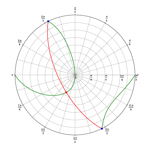
Figure 1: (Color online.) Visualization of the parameter space using polar coordinates. The radial axis shows the zenith angle $\theta$, while the (circular) polar axis shows the azimuth angle $\phi$, following the definition (50). Blue Points: $2c_{1}+c_{2}=c_{3}=0$, class $\mathrm{II}_{6}$, 6 polarizations; green line: $2c_{1}+c_{2}+c_{3}\neq 0,2c_{1}(c_{2}+c_{3})+c_{2}^{2}=0$, class $\mathrm{III}_{5}$, 5 polarizations; white area: $2c_{1}(c_{2}+c_{3})+c_{2}^{2}\neq 0,2c_{1}+c_{2}+c_{3}\neq 0$, class $\mathrm{N}_{3}$, 3 polarizations; red line: $2c_{1}+c_{2}+c_{3}=0,c_{3}\neq 0$, class $\mathrm{N}_{2}$, 2 polarizations.

We have visualized the aforementioned cases in figure 1, which we constructed as follows. We first made use of our assumption that at least one of the parameters $c_{1},c_{2},c_{3}$ is non-vanishing and introduced normalized parameters

$$\tilde{c}_{i}=\frac{c_{i}}{\sqrt{c_{1}^{2}+c_{2}^{2}+c_{3}^{2}}}$$ (49)

for $i=1,2,3$. One easily checks that the $\mathrm{E}(2)$ classes we found only depend on these normalized parameters. We then introduced polar coordinates $(\theta,\phi)$ on the unit sphere to express the parameters as

$$\tilde{c}_{1}=\sin\theta\cos\phi\,,\quad\tilde{c}_{2}=\sin\theta\sin\phi\,,\quad\tilde{c}_{3}=\cos\theta\,.$$ (50)

Since the $\mathrm{E}(2)$ class is the same for antipodal points on the parameter sphere, we restrict ourselves to the hemisphere $\tilde{c}_{3}\geq 0$, and hence $0\leq\theta\leq\frac{\pi}{2}$; this is equivalent to identifying antipodal points on the sphere and working with the projective sphere instead, provided that we also identify antipodal points on the equator $\tilde{c}_{3}=0$. We then considered $(\theta,\phi)$ as polar coordinates on the plane in order to draw the diagram shown in figure 1. Note that antipodal points on the perimeter, such as the two blue points, are identified with each other, since they describe the same class of theories.

This concludes our discussion of gravitational wave polarizations. We have seen that depending on the parameters $c_{1},c_{2},c_{3}$ we obtain the $\mathrm{E}_{2}$ class $\mathrm{II}_{6}$, $\mathrm{III}_{5}$, $\mathrm{N}_{3}$ or $\mathrm{N}_{2}$, with $\mathrm{N}_{3}$ filling most of the parameter space. We have also seen that there exists a family of theories besides TEGR which is of class $\mathrm{N}_{2}$ and thus exhibits the same two tensor modes as in general relativity. Theories in this class therefore cannot be distinguished from general relativity by observing the polarizations of gravitational waves alone.

V Conclusion

We studied the propagation of gravitational waves in the most general class of teleparallel gravity theories whose action is quadratic in the torsion tensor, known as new general relativity. The wave we considered is modeled as a linear perturbation of a diagonal tetrad corresponding to a Minkowski background metric. We derived the principal polynomial of the linearized field equations and found that gravitational waves propagate at the speed of light, i.e., their wave covector must be given by a null vector of the Minkowski background. Further, we made use of the Newman-Penrose formalism to derive the possible polarizations of gravitational waves. Our results show that the two tensor polarizations, which are present also in general relativity, are allowed for the whole class of theories we considered, while additional modes - two vector modes and up to two scalar modes - may be present for particular models within this class. We found that the teleparallel equivalent of general relativity is not the unique theory exhibiting exactly two polarizations, but there is a one-parameter family of theories with the same property. It thus follows that observations of gravitational wave polarizations may only give partial results on the parameter space of these theories.

We remark that although we restricted our analysis to theories whose action is quadratic in the torsion tensor, our results are valid for a significantly larger class of theories. This is due to the fact that the torsion is linear in the tetrad perturbations, so that the action is already quadratic in the perturbations. Hence, any higher order correction terms would have no influence on the linearized field equations. This observation agrees with previous results that there are no additional gravitational polarizations in $f(T)$ gravity compared to general relativity Bamba:2013ooa , since up to the required perturbation order the Lagrangian can be approximated as $f(T)=f(0)+f^{\prime}(0)T+\mathcal{O}(T^{2})$, which is equivalent to general relativity with a cosmological constant. An extension to the class of theories discussed in Bahamonde:2017wwk is shown in Hohmann:2018xnb .

Although higher order terms in the action do not influence the linear perturbations around a Minkowski background, they certainly have an influence on the cosmological dynamics of the theory, and therefore on the expansion history of the Universe. This modified expansion history might thus also leave an imprint on the observed gravitational waves propagating in a cosmological background. An interesting extension of our work would be to study gravitational waves as a perturbation to a tetrad corresponding to a Friedmann-Lemaitre-Robertson-Walker metric, taking into account modifications of the background dynamics arising from higher order torsion terms. Note that such modifications do not show up in the quadratic action we considered in this article, since all terms in the gravitational action become proportional to the square of the Hubble parameter in the case of cosmological symmetry, and so the action reduces to the teleparallel equivalent of general relativity, up to a constant factor.

Another possible class of extensions is to consider additional fields non-minimally coupled to torsion and to study their influence both on the speed and the polarization of gravitational waves. A canonical example is given by scalar-torsion theories Hohmann:2018rwf ; Hohmann:2018vle ; Hohmann:2018dqh ; Hohmann:2018ijr constructed from the TEGR torsion scalar and an additional scalar field, where one would expect the presence of an additional scalar mode compared to general relativity as it is also the case for scalar-curvature gravity. These theories can be extended by replacing the TEGR torsion scalar with the NGR torsion scalar which defined the Lagrangian considered in this article.

- (1) S. Nojiri and S. D. Odintsov, “Introduction to modified gravity and gravitational alternative for dark energy,” eConf C0602061 (2006) 06, arXiv:hep-th/0601213 [hep-th]. [Int. J. Geom. Meth. Mod. Phys.4,115(2007)].
- (2) S. Capozziello and M. De Laurentis, “Extended Theories of Gravity,” Phys. Rept. 509 (2011) 167–321, arXiv:1108.6266 [gr-qc].
- (3) A. Einstein, “Riemann-Geometrie mit Aufrechterhaltung des Begriffes des Fernparallelismus,” Sitzber. Preuss. Akad. Wiss. 17 (1928) 217–221.
- (4) T. Sauer, “Field equations in teleparallel spacetime: Einstein’s fernparallelismus approach towards unified field theory,” Historia Math. 33 (2006) 399–439, arXiv:physics/0405142 [physics].
- (5) C. Møller, “Conservation Laws and Absolute Parallelism in General Relativity,” K. Dan. Vidensk. Selsk. Mat. Fys. Skr. 1 (1961) no. 10, 1–50.
- (6) K. Hayashi and T. Nakano, “Extended translation invariance and associated gauge fields,” Prog. Theor. Phys. 38 (1967) 491–507.
- (7) Y. M. Cho, “Einstein Lagrangian as the Translational Yang-Mills Lagrangian,” Phys. Rev. D14 (1976) 2521.
- (8) K. Hayashi, “The Gauge Theory of the Translation Group and Underlying Geometry,” Phys. Lett. B69 (1977) 441.
- (9) R. Aldrovandi and J. G. Pereira, Teleparallel Gravity: An Introduction. Springer, Dordrechts, 2012.
- (10) J. W. Maluf, “The teleparallel equivalent of general relativity,” Annalen Phys. 525 (2013) 339–357, arXiv:1303.3897 [gr-qc].
- (11) R. Ferraro and F. Fiorini, “Modified teleparallel gravity: Inflation without inflaton,” Phys. Rev. D75 (2007) 084031, arXiv:gr-qc/0610067 [gr-qc].
- (12) R. Ferraro and F. Fiorini, “On Born-Infeld Gravity in Weitzenbock spacetime,” Phys. Rev. D78 (2008) 124019, arXiv:0812.1981 [gr-qc].
- (13) G. R. Bengochea and R. Ferraro, “Dark torsion as the cosmic speed-up,” Phys. Rev. D79 (2009) 124019, arXiv:0812.1205 [astro-ph].
- (14) E. V. Linder, “Einstein’s Other Gravity and the Acceleration of the Universe,” Phys. Rev. D81 (2010) 127301, arXiv:1005.3039 [astro-ph.CO]. [Erratum: Phys. Rev.D82,109902(2010)].
- (15) Y.-F. Cai, S. Capozziello, M. De Laurentis, and E. N. Saridakis, “f(T) teleparallel gravity and cosmology,” Rept. Prog. Phys. 79 (2016) no. 10, 106901, arXiv:1511.07586 [gr-qc].
- (16) Virgo, LIGO Scientific Collaboration, B. P. Abbott et al., “Observation of Gravitational Waves from a Binary Black Hole Merger,” Phys. Rev. Lett. 116 (2016) no. 6, 061102, arXiv:1602.03837 [gr-qc].
- (17) Virgo, LIGO Scientific Collaboration, B. P. Abbott et al., “GW170814: A Three-Detector Observation of Gravitational Waves from a Binary Black Hole Coalescence,” Phys. Rev. Lett. 119 (2017) no. 14, 141101, arXiv:1709.09660 [gr-qc].
- (18) L. Lombriser and A. Taylor, “Breaking a Dark Degeneracy with Gravitational Waves,” JCAP 1603 (2016) no. 03, 031, arXiv:1509.08458 [astro-ph.CO].
- (19) L. Lombriser and N. A. Lima, “Challenges to Self-Acceleration in Modified Gravity from Gravitational Waves and Large-Scale Structure,” Phys. Lett. B765 (2017) 382–385, arXiv:1602.07670 [astro-ph.CO].
- (20) S. Chakraborty, K. Chakravarti, S. Bose, and S. SenGupta, “Signatures of extra dimensions in gravitational waves from black hole quasinormal modes,” Phys. Rev. D97 (2018) no. 10, 104053, arXiv:1710.05188 [gr-qc].
- (21) J. Sakstein and B. Jain, “Implications of the Neutron Star Merger GW170817 for Cosmological Scalar-Tensor Theories,” Phys. Rev. Lett. 119 (2017) no. 25, 251303, arXiv:1710.05893 [astro-ph.CO].
- (22) J. M. Ezquiaga and M. Zumalacárregui, “Dark Energy After GW170817: Dead Ends and the Road Ahead,” Phys. Rev. Lett. 119 (2017) no. 25, 251304, arXiv:1710.05901 [astro-ph.CO].
- (23) T. Baker, E. Bellini, P. G. Ferreira, M. Lagos, J. Noller, and I. Sawicki, “Strong constraints on cosmological gravity from GW170817 and GRB 170817A,” Phys. Rev. Lett. 119 (2017) no. 25, 251301, arXiv:1710.06394 [astro-ph.CO].
- (24) Y. Akrami, P. Brax, A.-C. Davis, and V. Vardanyan, “Neutron star merger GW170817 strongly constrains doubly coupled bigravity,” Phys. Rev. D97 (2018) no. 12, 124010, arXiv:1803.09726 [astro-ph.CO].
- (25) T. Chiba, “1/R gravity and scalar - tensor gravity,” Phys. Lett. B575 (2003) 1–3, arXiv:astro-ph/0307338 [astro-ph].
- (26) C. Corda, “The production of matter from curvature in a particular linearized high order theory of gravity and the longitudinal response function of interferometers,” JCAP 0704 (2007) 009, arXiv:astro-ph/0703644 [astro-ph].
- (27) J. Naf and P. Jetzer, “On Gravitational Radiation in Quadratic Gravity,” Phys. Rev. D84 (2011) 024027, arXiv:1104.2200 [gr-qc].
- (28) L. Yang, C.-C. Lee, and C.-Q. Geng, “Gravitational Waves in Viable f(R) Models,” JCAP 1108 (2011) 029, arXiv:1106.5582 [astro-ph.CO].
- (29) K. Bamba, S. Capozziello, M. De Laurentis, S. Nojiri, and D. Sáez-Gómez, “No further gravitational wave modes in gravity,” Phys. Lett. B727 (2013) 194–198, arXiv:1309.2698 [gr-qc].
- (30) Y.-F. Cai, C. Li, E. N. Saridakis, and L. Xue, “ gravity after GW170817 and GRB170817A,” Phys. Rev. D97 (2018) no. 10, 103513, arXiv:1801.05827 [gr-qc].
- (31) H. Abedi and S. Capozziello, “Gravitational waves in modified teleparallel theories of gravity,” Eur. Phys. J. C78 (2018) no. 6, 474, arXiv:1712.05933 [gr-qc].
- (32) G. Farrugia, J. L. Said, V. Gakis, and E. N. Saridakis, “Gravitational Waves in Modified Teleparallel Theories,” Phys. Rev. D97 (2018) no. 12, 124064, arXiv:1804.07365 [gr-qc].
- (33) S. Bahamonde, C. G. Böhmer, and M. Wright, “Modified teleparallel theories of gravity,” Phys. Rev. D92 (2015) no. 10, 104042, arXiv:1508.05120 [gr-qc].
- (34) G. Kofinas and E. N. Saridakis, “Teleparallel equivalent of Gauss-Bonnet gravity and its modifications,” Phys. Rev. D90 (2014) 084044, arXiv:1404.2249 [gr-qc].
- (35) K. Hayashi and T. Shirafuji, “New general relativity,” Phys. Rev. D 19 (1979) 3524–3553. https://link.aps.org/doi/10.1103/PhysRevD.19.3524.
- (36) S. Bahamonde, C. G. Böhmer, and M. Krššák, “New classes of modified teleparallel gravity models,” Phys. Lett. B775 (2017) 37–43, arXiv:1706.04920 [gr-qc].
- (37) M. Hohmann, L. Järv, M. Krššák, and C. Pfeifer, “Teleparallel theories of gravity as analogue of non-linear electrodynamics,” Phys. Rev. D97 (2018) 104042, arXiv:1711.09930 [gr-qc].
- (38) T. Shirafuji, G. G. L. Nashed, and Y. Kobayashi, “Equivalence principle in the new general relativity,” Prog. Theor. Phys. 96 (1996) 933–948, arXiv:gr-qc/9609060 [gr-qc].
- (39) Yu. N. Obukhov and J. G. Pereira, “Teleparallel origin of the Fierz picture for spin-2 particle,” Phys. Rev. D67 (2003) 044008, arXiv:gr-qc/0212078 [gr-qc].
- (40) E. Newman and R. Penrose, “An Approach to gravitational radiation by a method of spin coefficients,” J. Math. Phys. 3 (1962) 566–578.
- (41) D. M. Eardley, D. L. Lee, A. P. Lightman, R. V. Wagoner, and C. M. Will, “Gravitational-wave observations as a tool for testing relativistic gravity,” Phys. Rev. Lett. 30 (1973) 884–886.
- (42) D. M. Eardley, D. L. Lee, and A. P. Lightman, “Gravitational-wave observations as a tool for testing relativistic gravity,” Phys. Rev. D8 (1973) 3308–3321.
- (43) M. Krššák and J. G. Pereira, “Spin Connection and Renormalization of Teleparallel Action,” Eur. Phys. J. C75 (2015) no. 11, 519, arXiv:1504.07683 [gr-qc].
- (44) M. Krššák and E. N. Saridakis, “The covariant formulation of f(T) gravity,” Class. Quant. Grav. 33 (2016) no. 11, 115009, arXiv:1510.08432 [gr-qc].
- (45) R. Ferraro and M. J. Guzmán, “Hamiltonian formulation of teleparallel gravity,” Phys. Rev. D94 (2016) no. 10, 104045, arXiv:1609.06766 [gr-qc].
- (46) Y. Itin, F. W. Hehl, and Y. N. Obukhov, “Premetric equivalent of general relativity: Teleparallelism,” Phys. Rev. D95 (2017) no. 8, 084020, arXiv:1611.05759 [gr-qc].
- (47) A. Golovnev, T. Koivisto, and M. Sandstad, “On the covariance of teleparallel gravity theories,” Class. Quant. Grav. 34 (2017) no. 14, 145013, arXiv:1701.06271 [gr-qc].
- (48) F. Müller-Hoissen and J. Nitsch, “Teleparallelism—a viable theory of gravity?,” Phys. Rev. D 28 (1983) 718–728. https://link.aps.org/doi/10.1103/PhysRevD.28.718.
- (49) J. Kuhfuss, R.and Nitsch, “Propagating modes in gauge field theories of gravity,” General Relativity and Gravitation 18 (1986) no. 12, 1207–1227. https://doi.org/10.1007/BF00763447.
- (50) L. Hörmander, The Analysis of Linear Partial Differential Operators I: Distribution Theory and Fourier Analysis. No. 256 in Grundlehren der mathematischen Wissenschaften. Springer, 1983.
- (51) L. Hörmander, The Analysis of Linear Partial Differential Operators II: Differential Operators with Constant Coefficients. No. 257 in Grundlehren der mathematischen Wissenschaften. Springer, 1983.
- (52) C. Pfeifer and D. Siemssen, “Electromagnetic potential in pre-metric electrodynamics: Causal structure, propagators and quantization,” Phys. Rev. D93 (2016) no. 10, 105046, arXiv:1602.00946 [math-ph].
- (53) P. Van Nieuwenhuizen, “On ghost-free tensor lagrangians and linearized gravitation,” Nucl. Phys. B60 (1973) 478–492.
- (54) C. M. Will, Theory and experiment in gravitational physics. 1993.
- (55) M. Hohmann, “Polarization of gravitational waves in general teleparallel theories of gravity,” Astron. Rep. 62 (2018) no. 12, 890–897, arXiv:1806.10429 [gr-qc].
- (56) M. Hohmann, L. Järv, and U. Ualikhanova, “Covariant formulation of scalar-torsion gravity,” Phys. Rev. D97 (2018) no. 10, 104011, arXiv:1801.05786 [gr-qc].
- (57) M. Hohmann, “Scalar-torsion theories of gravity I: general formalism and conformal transformations,” Phys. Rev. D98 (2018) no. 6, 064002, arXiv:1801.06528 [gr-qc].
- (58) M. Hohmann and C. Pfeifer, “Scalar-torsion theories of gravity II: theory,” Phys. Rev. D98 (2018) no. 6, 064003, arXiv:1801.06536 [gr-qc].
- (59) M. Hohmann, “Scalar-torsion theories of gravity III: analogue of scalar-tensor gravity and conformal invariants,” Phys. Rev. D98 (2018) no. 6, 064004, arXiv:1801.06531 [gr-qc].