Abstract

Modeling how individuals evolve over time is a fundamental problem in the natural and social sciences. However, existing datasets are often cross-sectional with each individual observed only once, making it impossible to apply traditional time-series methods. Motivated by the study of human aging, we present an interpretable latent-variable model that learns temporal dynamics from cross-sectional data. Our model represents each individual’s features over time as a nonlinear function of a low-dimensional, linearly-evolving latent state. We prove that when this nonlinear function is constrained to be order-isomorphic, the model family is identifiable solely from cross-sectional data provided the distribution of time-independent variation is known. On the UK Biobank human health dataset, our model reconstructs the observed data while learning interpretable rates of aging associated with diseases, mortality, and aging risk factors.

1 Introduction

Understanding how individuals evolve over time is an important problem in fields such as aging [Belsky et al., 2015], developmental biology [Waddington, 1940], cancer biology [Nowell, 1976], ecology [Jonsen et al., 2005], and economics [Ram, 1986]. However, observing large-scale temporal measurements of individuals is expensive and sometimes even impossible due to destructive measurements—e.g., in sequencing-based assays [Campbell and Yau, 2017]. As a result, we often only have cross-sectional data—each individual is only measured at one point in time (though different individuals can be measured at different points in time). From this data, we wish to learn longitudinal models that allow us to make inferences about how individuals change over time.

This paper is motivated by the problem of studying human aging using data from the UK Biobank, which contains extensive health data for half a million participants of ages 40–69 [Sudlow et al., 2015]. As an individual ages, many phenotypes change in correlated ways [McClearn, 1997]. Our goal is to find a low-dimensional latent representation of the phenotype feature space that captures the rates at which individuals change along each dimension as they age. To be scientifically useful—for instance, in understanding the genetic determinants of aging—these aging dimensions and rates should be interpretable (e.g., grouping phenotypically-related features together) and provably recoverable given some assumptions on the data.

The UK Biobank is unique among health datasets in its breadth and scale. However, most of its data is cross-sectional: 95% of its participants are measured at a single time point. Can we learn how individuals change over time purely from such cross-sectional data? While impossible in general [Hashimoto et al., 2016], this inference has been carried out in restricted settings, e.g., in single-cell RNA-seq studies [Campbell and Yau, 2017, Trapnell et al., 2014, Bendall et al., 2014]. However, those methods assume that individuals travel along the same single-dimensional trajectory, whereas human aging is a multi-dimensional process [McClearn, 1997]: someone might stay relatively physically fit but experience cognitive decline or vice versa (Figure 1). Other methods handle multi-dimensional latent processes (e.g., Wang et al. [2018]) but are concerned with inferring how the population evolves as a whole rather than with individual trajectories, and they do not provide guarantees on the interpretability or identifiability of the latent state.

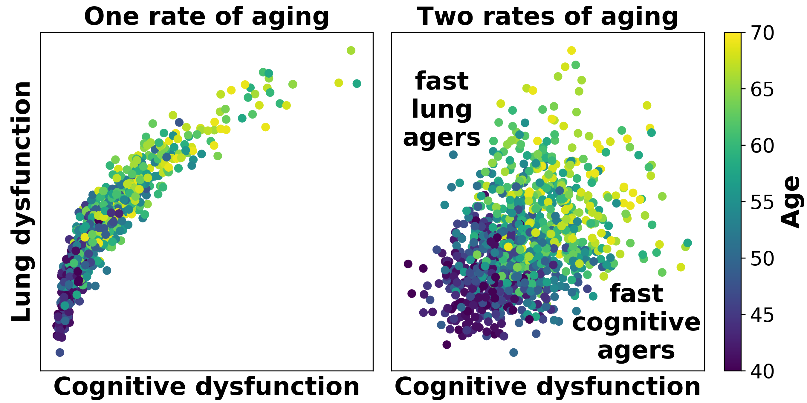
Figure 1: A toy example displaying multiple rates of aging (right) which allows individuals to progress rapidly in one aging dimension but not another.

In this paper, we introduce a method to learn a generative model of a multi-dimensional temporal process from cross-sectional data. We represent each individual by a low-dimensional latent state comprising a vector $rt$ that evolves linearly with time $t$ and a static bias vector $b$ that encodes time-independent variation. An individual’s observations are modeled as a non-linear function of their latent state $rt$ and $b$. In the aging context, each component of $r$ captures the age-dependent progression of different groups of phenotypes (e.g., muscle strength vs. cognitive ability), while $b$ captures age-independent individual variation.

We first study identifiability: under what conditions is it possible to learn the above model from the cross-sectional data that it generates? The key structure we leverage is the monotonicity of the mapping from the time-evolving state $rt$ to a subset of the observed features. This captures the intuition that aging is a gradual process where many systems show a generally-monotone decline after the age of 40, e.g., weight [Mozaffarian et al., 2011], red blood cells [Hoffmann et al., 2015], lung function [Stanojevic et al., 2008], and lean muscle mass [Goodpaster et al., 2006]. We prove that if the distribution of time-independent variation $b$ is known, a stronger version of monotonicity known as order isomorphism implies model identifiability (Section 3). Our work improves upon known identifiability results [Hashimoto et al., 2016] by giving identifiability results for the latent and non-ergodic cases. We also discuss how to optimize over monotone functions and check for order isomorphisms in our class of models, which is a computationally difficult question of independent interest (Section 4).

We assess our model using data from a subset of the UK Biobank: specifically, 52 phenotypes measured for more than 250,000 individuals with ages 40–69 (Section 7). Using this data, we learn an interpretable, low-dimensional representation of how human phenotypes change with age. This representation accurately reconstructs the observed data and predicts age-related changes in each phenotype. Through posterior inference on the rate vector $r$, we recover different dimensions of aging corresponding to different coordinates of $r$; these have natural interpretations as belonging to different body systems (e.g., cognitive performance and lung health). Consistent with biological knowledge, higher inferred rates of aging are associated with disease, mortality, and known risk factors (e.g., smoking).

2 Model

Let $x_{t}^{(i)}\in\mathbb{R}^{d}$ be the observed features of the $i$-th individual at time $t$. A classic approach to modeling temporal progression is to assume that $x_{t}^{(i)}$ depends linearly on some scalar, latent measure of progression $z_{t}^{(i)}\in\mathbb{R}$ (e.g., Klemera and Doubal [2006], Levine [2012], and Campbell and Yau [2017]). In the context of human aging, this scalar $z_{t}^{(i)}$ is often called biological age. We extend this approach in three ways: we allow $x_{t}^{(i)}$ to depend non-linearly on $z_{t}^{(i)}$ and a bias term; we constrain some components of $x_{t}^{(i)}$ to depend monotonically on $z_{t}^{(i)}$; and we allow $z_{t}^{(i)}$ to have multiple dimensions. Specifically, we characterize the $i$-th individual by two latent vectors:

1. A rate vector $r^{(i)}\in\mathbb{R}^{k_{\text{r}}}$ that determines how rapidly the $i$-th individual is changing over time.

2. A bias vector $b^{(i)}\in\mathbb{R}^{k_{\text{b}}}$ that encodes time-independent variation.

Each individual has their own values of $r^{(i)}$ and $b^{(i)}$ which do not change over time. For brevity, we will omit the $(i)$ superscript in the sequel unless explicitly comparing individuals.

We model each individual as evolving linearly in latent space at a rate proportional to $r$, i.e., $z_{t}=rt$, and we model $x_{t}$ as the sum of a time-dependent term $f(rt)$ and time-independent term $g(b)$:

$$x_{t}=f(rt)+g(b)+\epsilon.$$ (1)

Here, $f\colon\mathbb{R}^{k_{\text{r}}}\to\mathbb{R}^{d}$ is a non-linear function capturing time-dependent variation; $g\colon\mathbb{R}^{k_{\text{b}}}\to\mathbb{R}^{d}$ is a non-linear function capturing time-independent variation; and $\epsilon$ is measurement noise sampled i.i.d. at each time point. ${k_{\text{r}}}$ and ${k_{\text{b}}}$ are model hyperparameters. We assume that $r$, $b$, and $\epsilon$ are independently drawn from known priors, and that the rates $r$ are always positive.

Interpretation.

We interpret $z_{t}=rt$ as an individual’s ‘biological age’. In contrast to previous work, $z_{t}$ and $r$ are vector-valued quantities, capturing the intuition that aging is a multi-dimensional process (as discussed in Section 1). The function $f$ links the biological age $z_{t}$ with the observed features (phenotypes) $x_{t}$. The rate $r$ describes how quickly an individual ages along each latent dimension and differs between individuals, since different individuals experience age-related decline at different rates [McClearn, 1997]. The bias $b$ captures non-age-related variation like intrinsic differences in height, and also differs between individuals.

Monotonicity.

To ensure that the model is identifiable from cross-sectional data, we assume that some coordinates of $f$ are monotone. Roughly speaking, as $t$ increases, those coordinates of $f(rt)$ also increase on average; we defer a precise definition to Section 3. The monotonicity of $f$ is a reasonable assumption in the setting of human aging, as many features vary monotonically with age after the age of 40 [Mozaffarian et al., 2011, Hoffmann et al., 2015, Stanojevic et al., 2008, Goodpaster et al., 2006]. Monotonicity does not imply that, e.g., an individual’s strength has to strictly decrease with age (due to $\epsilon$) or that an older individual is always weaker than a younger one (because $g$ allows for age-independent variation between people).

For simplicity, we assume that the monotone phenotypes are known in advance. To streamline notation, we define $f$ to be monotone and have all non-monotone features modeled by some other unconstrained $\tilde{f}$, i.e., $x_{t}=[f(rt);\tilde{f}(rt)]+g(b)+\epsilon$.

Learning.

Our goal is to estimate $f$, $\tilde{f}$, $g$, and $\epsilon$ from cross-sectional data $\{(t^{(i)},x_{t^{(i)}}^{(i)})\}_{i=1}^{n}$. We parametrize the functions with neural networks and use a variational autoencoder to optimize a standard lower bound on the likelihood of the observed data [Kingma and Welling, 2014]; see Section 5 for more details.

3 Identifiability

We first study the basic question of identifiability: is it possible to recover $f$ (and thereby estimate temporal dynamics and rates of aging $r$) from cross-sectional data that is generated by $f$? In other words, do different $f$ give rise to different observed data?

Without loss of generality, we make two simplifications in our analysis. First, we only consider features $x$ that correspond to the monotone $f$, and disregard those which correspond to $\tilde{f}$; if the model is well-specified and can be identified just by considering $f$, then it will remain identifiable when additionally considering the non-monotone part $\tilde{f}$. Second, we consider a single noise term $\epsilon^{\prime}\stackrel{{\scriptstyle\rm def}}{{=}}g(b)+\epsilon$ which combines age independent variation $g(b)$ and the measurement noise $\epsilon$, since this does not affect the rate of aging. Together, these give the simplified model

$$x_{t} =f(rt)+\epsilon^{\prime},$$ (2)

where $x_{t}\in\mathbb{R}^{d}$ are the observed features, $r\in\mathbb{R}^{k_{r}}$ is the rate vector, and $t\in\mathbb{R}_{+}$ and $\epsilon^{\prime}\in\mathbb{R}$ are scalars. If $f$ is a general differentiable function without any monotonicity constraints, there exist functions that are unidentifiable from observations of the distribution of $x_{t}$. As an example, consider $\epsilon^{\prime}=0$ and $r\sim\text{lognormal}(0,1)$. Let $M$ be any matrix that preserves the all-ones vector $\mathbf{1}$ (i.e., $M\mathbf{1}=\mathbf{1}$) and is an orthogonal transform on the orthogonal subspace to $\mathbf{1}$. Since $\log(rt)\sim\mathcal{N}(\log t\mathbf{1},1)$, $M\log(rt)\overset{d}{=}\log(rt)$ due to the rotational invariance of the Gaussian (where $\overset{d}{=}$ means equality in distribution). This implies that $f(\exp(M\log(rt)))\overset{d}{=}f(rt)\overset{d}{=}x_{t}$. Since $f(\exp(M\log(\cdot)))$ and $f(\cdot)$ have the same observed distribution, they are indistinguishable from each other.

Therefore, we need to make additional assumptions on $f$ to ensure identifiability. Here, we will show that $f$ is identifiable up to permutation whenever the distribution of $\epsilon^{\prime}$ is known and both $f$ and $f^{-1}$ are monotone—that is, $f$ is an order isomorphism.

Definition 1.

A function $f$ is monotone if $u\preceq v\implies f(u)\preceq f(v)$ for all $u,v\in\text{dom}(f)$, where ordering is taken with respect to the positive orthant (i.e., $u\preceq v$ means $u_{i}\leq v_{i}$ for all $i$).

Definition 2.

An injective function $f$ is an order isomorphism if $f$ and $f^{-1}$ restricted to the image of $f$ are both monotone, that is, $u\preceq v\iff f(u)\preceq f(v)$.

3.1 Noiseless setting ($\epsilon^{\prime}=0$)

We begin by considering the case where $\epsilon^{\prime}=0$. Our main identifiability result is the following:

Proposition 1.

Let $x_{t}$ and $rt$ be the random variables defined in (2). If $f_{1}$ and $f_{2}$ and their inverses are twice continuously differentiable and are order-isomorphic functions such that $f_{1}(rt)\overset{d}{=}f_{2}(rt)\overset{d}{=}x_{t}$ for some $t>0$, then $f_{1}$ and $f_{2}$ are identical up to permutation.

We defer full proofs to Appendix A, but provide a short sketch here. The proof consists of two parts: we first show that all bijective order isomorphisms are permutations followed by component-wise monotone transforms. Then we show that any two maps $f_{1}$ and $f_{2}$ matching the observed data must be identical up to permutation.

Lemma 1.

If $q\colon\mathbb{R}^{k_{\text{r}}}\to\mathbb{R}^{k_{\text{r}}}$ is twice continuously differentiable and an order isomorphism, $q$ must be expressible as a permutation followed by a component-wise monotone transform.

We then consider the difference map $q\stackrel{{\scriptstyle\rm def}}{{=}}f_{2}^{-1}\circ f_{1}$, which maps the latent state implied by $f_{1}$ to that of $f_{2}$. $q$ is also an order isomorphism, so by Lemma 1 it is the composition of a permutation and monotone map. Since $f_{1}(rt)\overset{d}{=}f_{2}(rt)\overset{d}{=}x_{t}$, $q$ is measure preserving for $rt$. As the only monotone measure preserving map is the identity, $q$ must be a permutation.

3.2 Noisy setting ($\epsilon^{\prime}\neq 0$)

Identifiability in the noisy setting is more challenging. If the noise distribution $\epsilon^{\prime}$ is known, we can reduce the noisy setting to the noiseless setting by first taking the observed distribution of $x_{t}$ and then deconvolving $\epsilon^{\prime}$. This gives us the distribution of $f(x_{t})$, to which we can apply Proposition 1. The uniqueness of this procedure follows from the uniqueness of Fourier transforms and inverses over $L^{1}$ functions [Stein and Shakarchi, 2011]. This corresponds to the setting where we can characterize the distribution of the time-independent variation $g(b)$ and the measurement noise $\epsilon$, either through prior knowledge or measurement (e.g., in a controlled setting where we observe the starting point $x$ of all individuals). Importantly, we do not need to know the exact value of $b$ and $\epsilon$ for any individual, just their distributions.

If the noise distribution $\epsilon^{\prime}$ is unknown, then the characterization we provide here no longer holds, and we cannot simply deconvolve the noise. Nevertheless, we conjecture that the strong structure induced by monotonicity is sufficient for identifiability, and in simulations we are able to recover known ground-truth parameters (Section 6).

4 Learning order isomorphisms

Our identifiability results suggest that we should optimize for $f$ within the class of order isomorphisms. However, that optimization is difficult in practice, as it requires constraints on $f^{-1}$ that hold over the entire image of $f$. Instead, we take the following approach:

1. We relax the order isomorphism constraint and optimize for $f$ within a class of monotone transformations $\mathcal{M}$ that have a particular parametrization.

2. We check, post-hoc, if the learned $f\in\mathcal{M}$ is approximately order-isomorphic. (In real-world optimization settings, $f$ will not be exactly order-isomorphic for reasons we discuss below.) While not all functions in $\mathcal{M}$ are order-isomorphic, we choose $\mathcal{M}$ such that we can quickly verify if a given $f\in\mathcal{M}$ is approximately order-isomorphic.

While we do not have any prior expectation that the learned $f$ would be order-isomorphic, surprisingly, we find in our experiments (Section 5) that we do in fact learn an approximately order-isomorphic $f\in\mathcal{M}$. This suggests that we do not lose any representational power by moving from monotone functions to order-isomorphic functions, and that the assumption of order isomorphism (on top on monotonicity) is reasonable.

We choose $\mathcal{M}$ to be the set of functions that can be written as $f\colon\mathbb{R}^{k}\to\mathbb{R}^{d}=s_{2}\circ a\circ s_{1}$, where $s_{1}\colon\mathbb{R}^{k}\to\mathbb{R}^{k}$ and $s_{2}\colon\mathbb{R}^{d}\to\mathbb{R}^{d}$ are continuous, component-wise monotone transformations, and $a\colon\mathbb{R}^{k}\to\mathbb{R}^{d}$ is a linear transform. All $f\in\mathcal{M}$ are monotone by construction, due to the compositionality of monotone functions.

The following results show that we can check if some $f\in\mathcal{M}$ is order-isomorphic, i.e., $f^{-1}$ is also monotone, by examining only the linear transform $a$:

Lemma 2.

Let $a(v)=Av$ be a linear transform, where $A\in\mathbb{R}^{d\times k}$. If we can write $A=P\left[\begin{matrix}B\\ C\end{matrix}\right]$ where $P$ is a permutation matrix, $B$ is a non-negative monomial matrix, and $C$ is a non-negative matrix, then $a(\cdot)$ is an order isomorphism.

Proposition 2.

Let $f\colon\mathbb{R}^{k}\to\mathbb{R}^{d}=s_{2}\circ a\circ s_{1}$, where $s_{1}\colon\mathbb{R}^{k}\to\mathbb{R}^{k}$ and $s_{2}\colon\mathbb{R}^{d}\to\mathbb{R}^{d}$ are continuous, component-wise monotone transformations, and $a\colon\mathbb{R}^{k}\to\mathbb{R}^{d}$ is a linear transform. If $a$ satisfies Lemma 2, then $f$ is an order isomorphism.

See Appendix A.5 for proofs. Correspondingly, during training, we can restrict $f$ to the form $s_{2}\circ a\circ s_{1}$, where $s_{1}$ and $s_{2}$ are component-wise monotone transforms and $a$ is a linear transformation parametrized by $A$, a non-negative matrix. To check if the learned $f$ is order-isomorphic, Proposition 2 tells us that it suffices to check if $A$ satisfies the conditions of Lemma 2. Equivalently, each column of $A$ must have a non-zero element in a row where every other column has a zero.

Implementation.

The results above apply to linear transforms $a$ with pre- and post-transformations $s_{1}$ and $s_{2}$. In our experiments (Section 5), however, we found that using a single monotone component-wise transform ($f=s\circ a$) did not significantly harm performance. To help interpretability, we thus only use a single component-wise transform $s$. We parametrized $s$ as a polynomial with non-negative coefficients; this can be swapped for other differentiable parametrizations of monotone functions [Gupta et al., 2016]. This $f$ can be optimized during training by applying gradient descent to $A$ and the coefficients of $s$.

In our fitted model (Section 7), the learned $A$ was close to satisfying Lemma 2: each column $j$ contained at least one row $i$ where $A_{ij}\gg A_{ik}$ for all $k\neq j$ (specifically, $A_{ij}>50A_{ik}$). Thus, learning a monotone $f$ gave us an approximately monotone $f^{-1}$ without further constraints. This empirical finding was surprising to us and warrants future study, since learning an order-isomorphic $f$ would otherwise be computationally hard.

5 Experimental setup

Data processing.

Appendix B describes the full processing procedure. In brief, we selected features that were measured for a large proportion of participants, resulting in 52 phenotypes which we categorized by visual inspection into monotone (45/52) and non-monotone phenotypes (7/52). For convenience, we pre-processed the monotone phenotypes to all be monotone increasing with age by negating them if necessary. We use a train/development set of 213,510 individuals with measurements at a single time point, and report all results on a separate test set of 53,174 individuals not used in model development or selection. We also have longitudinal data from a single follow-up visit for an additional 8,470 individuals.

Model details.

We used a variational autoencoder to learn and perform inference in our model [Kingma and Welling, 2014]. Figure G.4 illustrates the model architecture. We parametrize the monotone function $f=s\circ a$ as the composition of a monotone elementwise transformation $s\colon\mathbb{R}^{d^{\prime}}\to\mathbb{R}^{d^{\prime}}$ with a monotone linear transform $a\colon\mathbb{R}^{k_{\text{r}}}\to\mathbb{R}^{d^{\prime}}$. As described in Section 4, we parametrized the linear transformation $a$ using a matrix $A$ constrained to have non-negative entries, and implemented each component $s_{i}(v)\colon\mathbb{R}_{+}\to\mathbb{R}_{+}$ of $s$ as the sum of positive powers of $v\in\mathbb{R}_{+}$ with non-negative coefficients $s_{i}(v)=\sum_{p_{j}\in S}w_{j}v^{p_{ij}}$, where $w_{ij}$ are learned non-negative weights, and $S$ is a hyperparameter. We verified that the learned model’s $A$ matrix can be row-permuted into a combination of an approximately monomial matrix and positive matrix, indicating that we learned an $f$ that was order-isomorphic (Section 4). For full details, see Appendix C. Our model implementation is publicly available: https://github.com/epierson9/multiphenotype_methods.

Hyperparameter selection.

We selected all hyperparameters other than the size of the latent states $k_{\text{r}}$ and $k_{\text{b}}$ (e.g., network architecture and the set of polynomials $S$) through random search evaluated on a development set (Appendix C). Increasing $k_{\text{r}}$ and $k_{\text{b}}$ gives the model more representational power; indeed, test ELBO increased uniformly with increasing $k_{\text{b}}$ and $k_{\text{r}}$ in the range we tested ($k_{\text{b}}+k_{\text{r}}\leq 20$). We chose $k_{\text{b}}=10$ and $k_{\text{r}}=5$ to balance modeling accuracy with dimensionality reduction for interpretability, since the test ELBO begins to level off at $k_{\text{r}}=5$; we chose a higher $k_{\text{b}}$ since we are not concerned with compressing the time-independent variation. Our results were similar with other values of $k_{\text{r}}$ and $k_{\text{b}}$ (Appendix F).

6 Results on synthetic data

To check if we could correctly recover the rates of aging $r$ in the well-specified setting, we generated synthetic data from a model and tried to recover the model parameters from that data.

We measured the quality of recovery by comparing the correlation between ground truth rates of aging $r_{\text{true}}$ and predicted individual rates of aging $r_{\text{fitted}}$. To generate realistic synthetic data, we fit the model described in Section 5 to data from the UK Biobank and then sampled from it (using the stated priors on $r$, $b$, and $\epsilon$). We verified that this synthetic data matched the properties of UK Biobank data, such as the age trends for each feature (Section 7 provides details). We ran this check for models with different values of $k_{\text{r}}=1,2,\dots,10$ and found good concordance across all values of $k_{\text{r}}$: the mean correlation between $r_{\text{fitted}}$ and $r_{\text{true}}$ was $0.91$ (averaged across values of $k_{\text{r}}$ and dimensions of $r$), and the slopes of the regressions of $r_{\text{fitted}}$ on $r_{\text{true}}$ were very close to one (mean absolute difference from 1 of 0.09), indicating good calibration.

These results suggest that if the model is well-specified, then it is identifiable even though the distribution of $g(b)+\epsilon$ is not known a priori. Moreover, our training procedure is able to recover the ground truth parameters quite closely.

7 Results on UK Biobank data

We first verify that our model fits the data (Section 7.1), before showing, as our main result, that it yields interpretable and biologically plausible rates of aging (Section 7.2). We compare to four baselines: principal components analysis (PCA); mixed-criterion PCA (mcPCA) [Bair et al., 2006]; contrastive PCA (cPCA) [Abid et al., 2018]; and our model with the monotone constraints removed and the same hyperparameter settings. We evaluate PCA, mcPCA, and cPCA using the same number of latent states as the original model ($k_{\text{r}}+k_{\text{b}}=15$); Appendix D provides full implementation details. (We discuss other potential baselines, and why they cannot be applied in our setting, in Section 8).

7.1 Reconstruction and extrapolation

We first show that our model can reconstruct each individual’s features from their low-dimensional latent state and extrapolate to future timepoints. The goal of these evaluations is not to demonstrate state-of-the-art predictive performance; rather, we want to verify that our model accurately reconstructs individual datapoints and captures aging trends.

Reconstruction.

We assessed whether our model was able to reconstruct observed datapoints from their latent space projections. Given an observation $(t,x_{t})$, we computed the approximate posterior mean of the latent variables $(\hat{r},\hat{b})$ using the encoder, and compared $x_{t}$ against the reconstructed posterior mean of $x_{t}$ given $(\hat{r},\hat{b})$. On a held-out test set, reconstruction was largely accurate, with a mean correlation between true and reconstructed feature values of 0.88 ( Figure G.6). The other baselines performed similarly: PCA, mcPCA, and cPCA did slightly worse, with mean correlations of 0.86, 0.86, and 0.84 respectively. The non-monotone model did slightly better (mean correlation 0.89); the small difference demonstrates that our monotone assumption does not undermine model fit.

Extrapolation to future timepoints.

To assess how accurately the model captures the dynamics of aging, we evaluate its ability to ‘fast-forward’ people through time: that is, to predict their phenotype $x_{t_{1}}$ at a future age $t_{1}$ given their current phenotype $x_{t_{0}}$ at age $t_{0}$. As above, we compute the posterior means $(\hat{r},\hat{b})$ using $x_{t_{0}}$ and $t_{0}$; we then predict $x_{t_{1}}=f(t_{1}\ \hat{r})+g(\hat{b})$. We do not compare to PCA, mcPCA, and cPCA on this task because they do not provide dynamics models, making it impossible to perform fast-forwarding.

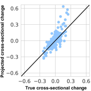
Figure 2: True and predicted changes are well-correlated ($r=0.77$) in cross-sectional data when fast-forwarding 5 years. Each point represents difference in one feature for one 5-year age bin: e.g., difference in heart rate between 40–45 and 45–50 year olds.

We assess the accuracy of fast-forwarding on both cross-sectional and longitudinal data. On cross-sectional data, we do not have follow-up data $x_{t_{1}}$ for each person, so we evaluate the model by age group: for example, we fast-forward all 40–45 year olds by 5 years, compute how much the model predicts each feature will change on average, and compare that to the true average feature change between 40–45 year olds and 45–50 year olds. (Although we bucket age in this analysis to reduce noise, the model uses the person’s exact age.) Predictions are highly correlated with the true values ($r=0.77$ for 5-year follow-ups, Figure 2; $r=0.88$ for 10 years, and $0.94$ for 15 years. This is similar to the performance of the non-monotone baseline, which achieves correlations of $0.77,0.90$, and $0.96$ for 5, 10, and 15 years.

On longitudinal data, we observe both $x_{t_{0}}$ and $x_{t_{1}}$ for a single person, and can therefore use reconstruction accuracy of $x_{t_{1}}$ as a metric. This task is difficult because longitudinal follow-up times are very short in our dataset (2–6 years), so aging-related changes may be swamped by the inherent noise in the task and sampling biases in the longitudinal cohort. We compare to three additional baselines on this task: predicting no change, $x_{t_{1}}=x_{t_{0}}$; reconstructing $x_{t_{0}}$ without fast-forwarding, $x_{t_{1}}=f(t_{0}\ \hat{r})+g(\hat{b})$; and fast forwarding according to the average rate of change in the cross-sectional data. Our evaluation metric is the fraction of people for which our model yields lower reconstruction error than each baseline. For follow-up times long enough to allow for substantial age-related change (${\geq 5}$ years), our model predicts $x_{t_{1}}$ more accurately than all three benchmarks on most individuals (Table 1, top row), and performs comparably, though slightly worse, than the non-monotone model (Table 1, bottom row). Appendix E describes a natural extension of our model which allows both longitudinal and cross-sectional data to be used in model fitting, which significantly improves performance on this task.

Table 1: % of people for which the rate-of-aging models predict $x_{t_{1}}$ more accurately than do benchmarks.

Benchmark methods:	$x_{t_{0}}$	Recons. $x_{t_{0}}$	avg $\Delta$
Monotone	66%	61%	60%
Non-monotone	71%	63%	65%

The results above show that our model reconstructs the observed data slightly more accurately than linear methods (PCA, cPCA, and mcPCA) while providing an accurate dynamics model, which these linear methods do not. Moreover, the monotonicity assumption does not hurt our model’s performance too much.

7.2 Model interpretation

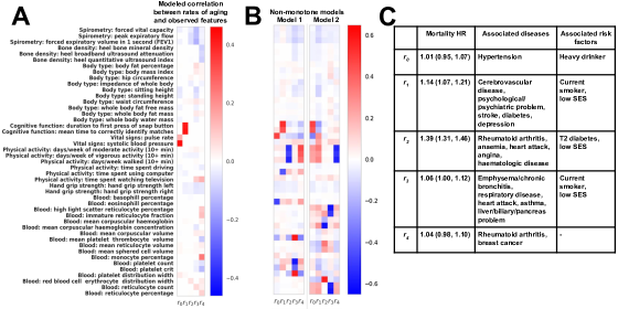
Figure 3: A: Model-learned correlations between rates of aging $r$ (columns) and observed features $x$ (rows) for monotone features. Each cell displays the correlation between one rate of aging and one observed feature in data sampled from the model. Learned rates of aging are sparse and stable across runs and hyperparameter settings; in contrast, without monotone constraints (B) the rates of aging are not sparse or stable. C: Associations with mortality, diseases, and rate-of-aging risk factors. Mortality HR is the hazard ratio for a one-std-dev increase in rate of aging in a Cox proportional hazards model. The final two columns list the diseases and risk factors most strongly positively associated with higher rates of aging. We list up to five significant ($p<0.05$ after Bonferroni correction) and strong (effect size $>$ 1% increase in the rate of aging) associations for each rate.

Our main experimental result is that we obtain interpretable rates of aging from our monotone model. In particular, we found that enforcing monotonicity in $f$ encouraged sparsity. To interpret the rates of aging $r$, we simply associated each component of $r$ with the sparse set of features that it correlated with (Figure 3A). These rates were more interpretable than those learned by the four baselines: the model without monotone constraints and PCA, cPCA, and mcPCA. Without the monotone constraints (Figure 3B) the rates are not associated with sparse sets of features and are less interpretable. Further, because the rates of aging $r$ in the non-monotone model can be rotated without affecting model fit, the model is unstable, learning different rates $r^{(i)}$ for the same individual $i$ when trained with different random seeds. Figure 3B shows that the top two non-monotone models (by test ELBO) learn very different $r$’s. To compare two models, we defined $\rho_{r}$ as the correlation between the $r^{(i)}$’s learned by the two models, averaged over each component of $r$, and maximized over permutations of components. For the top two non-monotone models, $\rho_{r}$ was only 0.44, vs. $\rho_{r}=0.94$ for the top two monotone models. The monotone model was also stable over changes to the number of non-monotone features, random subsets of the training data, and the dimensions $k_{r}$ and $k_{b}$ of the time-dependent and bias latent variables (Appendix F). This demonstrates empirically that, consistent with our theoretical results, monotonicity is essential to learning stable and interpretable rates of aging.

Similarly, the latent factors learned by the three linear baselines (PCA, cPCA, and mcPCA) were difficult to interpret because they did not clearly distinguish between time-dependent and time-independent variation and were not sparse (Appendix Figure G.7). For example, the first principal component learned by PCA was most strongly associated with body type (e.g., height and weight), but this mostly captures the variation in body type within age groups, and is only weakly correlated ($\rho=0.13$) with age. None of the top 5 principal components learned by any of the three methods had an absolute correlation with age of greater than 0.3.

To assess the biological plausibility of our learned rates of aging, we examined associations between each rate of aging and three external sets of covariates not used in fitting the model: mortality; 91 diseases; and 5 risk factors which are known to accelerate aging processes, such as being a current smoker. We show these associations in Figure 3C (see Appendix B for details). Rates of aging were positively associated with all three sets of covariates: of the 88 statistically significant associations with diseases ($p<0.05$ after Bonferroni correction), 78% were positive; 73% of the 15 statistically associations with risk factors were positive, and all associations with mortality were positive although—interestingly—to widely varying degrees.

Based on these associations, we interpret the rates of aging $r$ as follows: $r_{0}$, a ‘blood pressure rate of aging’, associates with blood pressure; $r_{1}$, a ‘cognitive rate of aging’, associates with the two cognitive function phenotypes and with cognitive diseases (e.g., psychiatric problems and strokes); $r_{2}$ associates with heart conditions including heart attacks and angina and is the most strongly associated with mortality; $r_{3}$, a ‘lung rate of aging’, associates with pulmonary function and lung diseases (e.g., bronchitis and asthma), and is elevated in smokers; and $r_{4}$, a ‘blood and bone rate of aging’, correlates with blood phenotypes (e.g., monocyte percentage) and rheumatoid arthritis, an autoimmune disorder associated with changes in monocyte and platelet levels [Milovanovic et al., 2004, Rossol et al., 2012]. Interestingly, $r_{4}$ also correlates with the bone density phenotypes, a direction for future study.

8 Related work

Biological age.

In our work, we interpreted the vector $rt$ as the ‘biological age’ of an individual. The notion of biological age as a measurable quantity that tracks chronological age on average but captures an individual’s ‘true age’ dates back 50 years [Comfort, 1969]. It is common to regress chronological age against a set of phenotypes and call the predicted quantity biological age [Furukawa et al., 1975, Borkan and Norris, 1980, Klemera and Doubal, 2006, Levine, 2012, Horvath, 2013, Chen et al., 2016, Putin et al., 2016]. These methods estimate a single-dimensional biological age and do not allow for longitudinal inferences. Belsky et al. [2015] estimates a single-dimensional rate of aging, but requires longitudinal data.

Pseudotime methods in molecular biology.

These methods order biological samples (for example, microarray data [Magwene et al., 2003, Gupta and Bar-Joseph, 2008] or RNA-seq data [Reid and Wernisch, 2016, Kumar et al., 2017]) using their gene expression levels; the imputed temporal order is referred to as pseudotime. These methods typically use either some form of minimum spanning tree [Qiu et al., 2011, Trapnell et al., 2014, Bendall et al., 2014] or a Bayesian approach [Campbell and Yau, 2017, Äijö et al., 2014], under the assumption of a single-dimensional temporal trajectory (with discrete branching points). Gupta and Bar-Joseph [2008] showed recoverability of such methods under similar assumptions.

Dimensionality reduction.

Others have studied aging on cross-sectional data using dimensionality reduction (DR) methods such as PCA [Nakamura et al., 1988] and factor analysis [MacDonald et al., 2004], using the first factor as the ‘aging dimension’. These methods do not explicitly take temporal information into account, and therefore do not cleanly factor out time-dependent changes from time-independent changes. DR methods specific to time-series data, such as functional PCA, have been used to study clinically-relevant changes over time [Di et al., 2009, Greven et al., 2011] but require longitudinal data.

Recovery of individual dynamics from cross-sectional data.

Recovering the behavior of individuals from population data has been studied as ‘ecological inference’ [King, 2013] or ‘repeated cross-section’ analysis [Moffitt, 1993, Collado, 1997, Kalbfleisch and Lawless, 1984, Plas, 1983, Hawkins and Han, 2000, Bernstein and Sheldon, 2016]. These works focus on models without latent variables and are restricted to linear or discrete time-series. Hashimoto et al. [2016] consider learning dynamics from cross-sectional data in more general settings, but do not consider latent variable inference; moreover, their method relies on observing nearly-stationary data, which is inapplicable to our setting. Wang et al. [2018] uses a latent-variable model to infer population evolution, and can also be applied to modeling individuals. However, because their main goal is population dynamics, their latent variables are not designed to be interpretable or identifiable.

Monotone function learning.

The task of learning partial monotone functions has been well-studied [Gupta et al., 2016, Daniels and Velikova, 2010, Qu and Hu, 2011, You et al., 2017]. The difficulty in applying these to our setting is that we need $f$ to have a specific parametric form for efficient order-isomorphism checking (Section 4), which these methods do not satisfy. It is an open question if these methods can be adapted to learning order isomorphisms.

9 Discussion

We have presented a method to learn, from cross-sectional data, a low-dimensional latent representation of how people change as they age. Empirically, this representation is interpretable and biologically plausible, allowing us to infer an individual’s rates of aging along each dimension of the latent space. Theoretically, we leverage the order isomorphism of the mapping between the latent space and the observed phenotypes to show that our model family is identifiable. To learn an order-isomorphic mapping—which is computationally intractable in general—we introduce a parametric mapping that is easily verifiable as order-isomorphic, and show through experiments that this parametrization automatically learns an order isomorphism on our data.

Our model opens up many directions for future work. We could extend it to incorporate more complexities of real-world data, including survivorship bias [Fry et al., 2017, Louis et al., 1986] or discontinuous changes in latent state (e.g, damage caused by a heart attack). Powerful previous ideas in latent variable models—for example, discrete latent variables [Jang et al., 2017, Maddison et al., 2016] that capture phenomena like sex differences—could be used to relax the model’s parametric assumptions. Incorporating genetic information also represents a promising direction for future work. For example, genotype information could be used to learn rates of aging with a stronger genetic basis.

We anticipate that our learned rates of aging will be useful in downstream tasks like genome-wide association studies, where combining multiple phenotypes can increase power [O’Reilly et al., 2012]. Finally, we hope that our model, by offering an interpretable multi-dimensional characterization of temporal progression, can be applied to longitudinal inference in other domains, like single-cell analysis and disease progression.

Acknowledgments

We thank Zhenghao Chen, Jean Feng, Adam Freund, Noah Goodman, Mitchell Gordon, Steve Meadows, Baharan Mirzasoleiman, Chris Olah, Nat Roth, Camilo Ruiz, Christopher Yau, and the Calico UK Biobank team for helpful discussion. EP was supported by the Hertz and NDSEG Fellowships and PWK was supported by the Facebook Fellowship.

Appendix A Proofs

A.1 Non-negative and monomial matrices

In this section, we show that if the inverse of a non-negative matrix $A$ exists and is itself non-negative, then $A$ has to be a monomial matrix. This is a known linear algebra fact; we provide a proof for completeness, adapted from [EuYu, 2012].

Definition 3.

A matrix $A$ is called a non-negative matrix if all of its elements are ${\geq 0}$, and a positive matrix if all of its elements are ${>0}$.

Definition 4.

A matrix $A$ is called a monomial matrix if it has exactly one non-zero entry in each row and each column. In other words, it has the same sparsity pattern as a permutation matrix, though the non-zero elements are allowed to differ from one.

Lemma 3.

If $A$ is an invertible non-negative matrix and $A^{-1}$ is also non-negative, then $A$ must be a non-negative monomial matrix.

Proof.

Since $A$ is invertible, every row of $A$ must have at least one non-zero element. Consider the $i$-th row of $A$, and pick $j$ such that $A_{ij}\neq 0$. Since $AA^{-1}=I$, we have that the dot product of the $i$-th row of $A$ with the $k$-th column of $A^{-1}$ must be 0 for all $i\neq k$. As $A$ and $A^{-1}$ are both non-negative, this dot product can only be 0 if every term in it is 0, including the product of $A_{ij}$ with $A^{-1}_{jk}$. However, $A_{ij}\neq 0$ by construction, so $A^{-1}_{jk}$ must be 0 for all $i\neq k$. In other words, the $j$-row of $A^{-1}$ must be all 0 except for $A^{-1}_{ji}$.

Applying a symmetric argument, we conclude that the $i$-th row of $A$ must be all 0 except for $A_{ij}$. Since this holds for all $i$, we have that $A$ must have exactly one non-zero in each row. Moreover, these non-zeros must appear in distinct columns, else $A$ would be singular. We thus conclude that $A$ must be a monomial matrix. ∎

A.2 The Jacobians of monotone and order isomorphic functions

We recall the definition of monotone and order isomorphic functions from the main text:

Definition 1.

A function $f$ is monotone if $u\preceq v\implies f(u)\preceq f(v)$ for all $u,v\in\text{dom}(f)$, where ordering is taken with respect to the positive orthant (i.e., $u\preceq v$ means $u_{i}\leq v_{i}$ for all $i$).

Definition 2.

An injective function $f$ is an order isomorphism if $f$ and $f^{-1}$ restricted to the image of $f$ are both monotone, that is, $u\preceq v\iff f(u)\preceq f(v)$.

In this section, we establish that monotonicity and order isomorphism impose strong constraints on the function Jacobians.

Lemma 4.

If a function $f\colon\mathbb{R}^{k_{\text{r}}}\to\mathbb{R}^{k_{\text{r}}}$ is twice differentiable and monotone, then the Jacobian of $f$ evaluated at any $z\in\mathbb{R}^{k_{\text{r}}}$ is a non-negative matrix.

Proof.

Assume for contradiction that $f$ is differentiable and monotone, but that there exists some $z\in\mathbb{R}^{k_{\text{r}}}$ such that the Jacobian $J_{f}(z)$ is not a non-negative matrix. By definition, this implies that we can find $i$ and $j$ such that the $ij$-th entry of $J_{f}(z)$ is negative.

Let $e_{j}$ represent the $j$-th unit vector. By the remainder bound for Taylor approximations, twice differentiability implies that for any compact ball around $z$, we can find some constant $M$ such that we can write $f(z+\delta e_{j})\leq f(z)+\delta J_{f}(z)e_{j}+\frac{M}{2}\delta^{2}$. If we pick $\delta<2|J_{f}(z)_{ij}|/M$, the first order term dominates. Since the $ij$-th entry is negative, this means that $f_{i}(z+\delta e_{j})<f_{i}(z)$ even though $z+\delta e_{j}\succeq z$, contradicting the monotonicity of $f$. ∎

Lemma 5.

If $q\colon\mathbb{R}^{k_{\text{r}}}\to\mathbb{R}^{k_{\text{r}}}$ is twice continuously differentiable and an order isomorphism, then the Jacobian matrix $J_{h}(z)$ is a non-negative monomial matrix for all $z\in\mathbb{R}^{k_{\text{r}}}$.

Proof.

If $q$ is an order isomorphism, then $q$ and $q^{-1}$ are both monotone. By Lemma 4, their respective Jacobian matrices are non-negative everywhere.

Now, for any $z\in\mathbb{R}^{k_{\text{r}}}$, the inverse function theorem tells us that ${[J_{q}(z)]}^{-1}=J_{q^{-1}}(q(z))$, so both $J_{q}(z)$ and its inverse ${[J_{q}(z)]}^{-1}$ are non-negative. Applying Lemma 3 gives us that $J_{q}(z)$ is a non-negative monomial matrix. ∎

A.3 Component-wise monotonicity of order isomorphisms

The conditions on the Jacobian of a twice differentiable order isomorphic function $q$ imply a constrained form.

Lemma 1 (restated).

If $q\colon\mathbb{R}^{k_{\text{r}}}\to\mathbb{R}^{k_{\text{r}}}$ is an order isomorphism and twice continuously differentiable, $q$ must be expressible as a permutation followed by a component-wise strictly monotone transform.

Proof.

Since $q$ is bijective, $q^{-1}$ exists everywhere, which implies that $J_{q}(r)$ must have full rank everywhere. Since $J_{q}(r)$ is a monomial matrix by Lemma 5, this means that the sparsity pattern of $J_{q}(r)$ cannot vary with $r$; otherwise, by the intermediate value theorem, there will be some $r$ where $J_{q}(r)$ where a row has greater than one nonzero or no nonzeros and thus is not monomial. By definition, a monomial matrix can be decomposed into a positive diagonal matrix and a permutation. Applying the fundamental theorem of calculus to each diagonal entry recovers the strictly monotone tranform, and the permutation matrix defines the permutation. The existence of the antiderivative is guaranteed by construction of $J_{q}$ as the derivative of $q$. ∎

A.4 Identifiability in the noiseless setting

We start by establishing two helpful lemmas:

Lemma 6.

If functions $f_{1}$ and $f_{2}$ are both monotone, then $f_{1}\circ f_{2}$ is also monotone.

If $f_{1}$ and $f_{2}$ are both bijective order isomorphisms, then $q\stackrel{{\scriptstyle\rm def}}{{=}}f_{2}^{-1}\circ f_{1}$ is also a bijective order isomorphism.

Proof.

The first part of the lemma follows from the transitivity of partial orders: $x\prec y\implies f_{1}(x)\prec f_{1}(y)\implies f_{2}(f_{1}(x))\prec f_{2}(f_{1}(x))$.

For the second part, note that $q$ is bijective because it is the composition of two bijective functions. Now, since $f_{1}$ and $f_{2}$ are both order isomorphisms, we know that $f_{1},f_{1}^{-1},f_{2}$, and $f_{2}^{-1}$ are all monotone. By the first part of the lemma, we conclude that $q=f_{2}^{-1}\circ f_{1}$ and $q^{-1}=f_{1}^{-1}\circ f_{2}$ are both monotone, implying that $q$ is an order isomorphism. ∎

Lemma 7.

If a continuous, univariate, strictly monotone function $q_{i}$ is measure preserving for a random variable $x$, $q_{i}$ must be the identity map (on the support of $x$).

Proof.

By strict monotonicity, $c_{1}<c_{2}$ implies $q(c_{1})<q(c_{2})$ and thus the CDF is preserved implying that $P(x<c)=P(q(x)<q(c))=P(x<q(c))$. The last step follows from measure preservation of $q$.

Now assume for contradiction that $q_{i}$ is not the identity map. We can then pick some $c$ such that $q(c)\neq c$ and $P(c)>0$. This implies that $P(x<q(c))\neq P(x<c)$ which is a contradiction. ∎

We can now state and prove identifiability in the noiseless setting:

Proposition 1 (restated).

If $f_{1}$ and $f_{2}$ and their inverses are twice continuously differentiable and order-isomorphic functions such that $f_{1}(tr)\overset{d}{=}f_{2}(tr)\overset{d}{=}x_{t}$ for some $t>0$, then $f_{1}$ and $f_{2}$ are identical up to a permutation.

Proof.

We consider the difference map $q\stackrel{{\scriptstyle\rm def}}{{=}}f_{2}^{-1}\circ f_{1}$, which maps latent rates of aging implied by $f_{1}$ to that of $f_{2}$. Our aim is to show that $q$ must be a permutation, which will give the desired result.

From Lemma 6, we know that $q$ is itself an order isomorphism. Thus, by Lemma 1, it must be expressible as the composition of a component-wise strictly monotone map and a permutation.

We can further show that this component-wise strictly monotone transformation has to be the identity transformation. Since both $f_{1}$ and $f_{2}$ map $rt\mapsto x_{t}$, $q$ is measure preserving on $rt$. In other words, it maps the probability distribution of $rt$ to itself. We can therefore apply Lemma 7 to conclude that $q$ can only be a permutation.

Applying $f_{2}$ to both sides of $q=f_{2}^{-1}\circ f_{1}$, we get that $f_{1}$ and $f_{2}$ have to be permutations of each other, as desired. ∎

A.5 Checking order isomorphisms

Lemma 2 (restated).

Let $a(x)=Ax$, where $A\in\mathbb{R}^{d\times k}$. If we can write $A=P\left[\begin{matrix}B\\ C\end{matrix}\right]$ where $P$ is a permutation matrix, $B$ is a non-negative monomial matrix, and $C$ is a non-negative matrix, then $a$ is an order isomorphism.

Proof.

$a$ is monotone since $A$ is non-negative. To verify that the inverse of $a$ over its image is monotone, let $I_{k}=[I;0]\in\mathbb{R}^{k\times d}$ be the matrix selecting the first $k$ coordinates. If $Ax\prec Ay$, every coordinate of $Ax$ is smaller than the corresponding coordinate of $Ay$, so we can jointly permute the rows (i.e., left-multiplying by a permutation matrix) or select a subset of coordinates while preserving ordering. Thus, $Ax\prec Ay\implies I_{k}P^{-1}Ax\prec I_{k}P^{-1}Ay$. By construction, $I_{k}P^{-1}A=B$ is a non-negative monomial matrix. Applying a similar permutation argument, we have that $I_{k}P^{-1}Ax\prec I_{k}P^{-1}Ay\implies x\prec y$. ∎

Proposition 2 (restated).

Let $f\colon\mathbb{R}^{k}\to\mathbb{R}^{d}=s_{2}\circ a\circ s_{1}$, where $s_{1}\colon\mathbb{R}^{k}\to\mathbb{R}^{k}$ and $s_{2}\colon\mathbb{R}^{d}\to\mathbb{R}^{d}$ are continuous, component-wise monotone transformations, and $a\colon\mathbb{R}^{k}\to\mathbb{R}^{d}$ is a linear transform. If $a$ satisfies Lemma 2, then $f$ is an order isomorphism.

Proof.

The proof follows from the fact that order preservation is transitive. $a\circ s_{1}$ is an order isomorphism onto its image, since $s_{1}$ is an order isomorphism on the entire $\mathbb{R}^{k}$ and $a$ is order isomorphic onto its image by Lemma 2. Thus for any $x\prec y\iff a(s_{1}(x))\prec a(s_{1}(y))$. Since $s_{2}$ is an order isomorphism on $\mathbb{R}^{d}$, we have $x\prec y\iff a(s_{1}(x))\prec a(s_{1}(y))\iff s_{2}(a(s_{1}(x)))\prec s_{2}(a(s_{1}(y)))$. ∎

Appendix B UK Biobank dataset and processing

Phenotype filtering.

We selected Biobank phenotypes that were measured for a large proportion of the dataset and that captured diverse and important dimensions of aging and general health. After removing phenotypes which were missing data for many people, redundant (e.g., there are multiple measurements of BMI), or discrete (e.g., categorical responses from a survey question), we were left with 52 phenotypes (Table 2) across the following categories: spirometry (a measure of lung function), bone density, body type/anthropometry, cognitive function, vital signs (blood pressure and heart rate), physical activity, hand grip strength, and blood test results. By visual inspection, we categorized the 52 phenotypes into monotone features (45/52) and non-monotone features (7/52) for the cross-sectional model. In the combined longitudinal/cross-sectional model, we modeled an additional 8 features as non-monotone because they increased in the longitudinal data but not in the cross-sectional data, or vice versa.

Sample filtering.

We removed individuals with non-European ancestry, as identified from their genetic principal components, as is commonly done in studies of the UK Biobank to minimize spurious correlations with ancestry particularly in genetic analysis [Lane et al., 2016, Wain et al., 2015]. (The vast majority of individuals in UK Biobank are of European ancestry.) We also removed individuals who were missing data in any of our selected phenotypes.

After filtering, we were left with a train/development set of 213,510 individuals; we report all results on a test set of 53,174 individuals not used in model development or selection. While these samples are cross-sectional (with a measurement at only a single timepoint), we have a single longitudinal followup visit for an additional 8,470 individuals, on which we assess longitudinal progression. UK Biobank data contains two followup visits; we use only longitudinal data from the first followup visit (2-6 years after the initial visit), not the second, because some of the phenotypes we use in model fitting were not measured at the second followup.

Phenotype processing.

We normalized each phenotype to have mean 0 and variance 1. In fitting the model, we first transformed all phenotypes so they were positively correlated with age, by multiplying all phenotypes which were not by negative one, so we could assume that monotone features were monotone increasing. However, all results in the paper are shown with the original phenotype signs.

Diseases, mortality, and risk factors.

We examined associations with 91 diseases which were reported by at least 5,000 individuals in the entire UKBB dataset. Diseases were retrospectively assessed via interview (i.e., subjects developed the disease prior to the measurement of $x_{t_{0}}$). Second, we examined associations between rates of aging and mortality. In contrast to disease status, mortality was measured after $x_{t_{0}}$ (all subjects were obviously alive when $x_{t_{0}}$ was measured); thus, examining associations with mortality serves as an indication that rates of aging predict future outcomes. Finally, we examined 5 binary risk factors: whether the individual currently smokes, if they are a heavy drinker, if they are above the 90th percentile in Townsend deprivation index (a measure of low socioeconomic status), if they have type 2 diabetes, and if they report no days of moderate or vigorous exercise in a typical week.

We examined associations between rates of aging and mortality using a Cox proportional hazards model which controlled for age, sex, and the first five genetic principal components. We report the hazard ratios for a one standard-deviation increase in rate of aging. For the 5 binary risk factors and the 91 diseases, we examined associations using a linear regression model, where the dependent variable was the rate of aging and the independent variable was the risk factor or disease. We controlled for age, sex, and the first five genetic principal components. We filtered for associations which passed a statistical significance threshold of $p=0.05$, with Bonferroni correction for the number of tests performed. Figure 3 reports the diseases/risk factors with the largest positive associations and an effect size of a greater than 1% increase in the rate of aging; if more than five diseases or risk factors pass this threshold, we report the top five.

Table 2: UK Biobank features used in model fitting. * denotes features which are modeled as non-monotone in age when fitting the cross-sectional model. ** denotes additional features which are modeled as non-monotone in age when fitting the model which uses both longitudinal and cross-sectional data. All features which are modeled as non-monotone in the cross-sectional analysis are also modeled as non-monotone in the combined longitudinal/cross-sectional model.

Feature
Spirometry: forced vital capacity
Spirometry: peak expiratory flow
Spirometry: forced expiratory volume in 1 second (FEV1)
Bone density: heel bone mineral density
Bone density: heel broadband ultrasound attenuation
Bone density: heel quantitative ultrasound index
Body type: body fat percentage
Body type: body mass index
Body type: hip circumference
Body type: impedance of whole body**
Body type: sitting height
Body type: standing height
Body type: waist circumference
Body type: whole body fat free mass
Body type: whole body fat mass
Body type: whole body water mass
Cognitive function: duration to first press of snap button
Cognitive function: mean time to correctly identify matches
Vital signs: diastolic blood pressure*
Vital signs: pulse rate**
Vital signs: systolic blood pressure
Physical activity: days/week of moderate activity (10+ min)
Physical activity: days/week of vigorous activity (10+ min)
Physical activity: days/week walked (10+ min)
Physical activity: time spent driving
Physical activity: time spent using computer**
Physical activity: time spent watching television
Hand grip strength: hand grip strength left
Hand grip strength: hand grip strength right
Blood: basophil percentage
Blood: eosinophil percentage
Blood: haematocrit percentage*
Blood: haemoglobin concentration*
Blood: high light scatter reticulocyte percentage
Blood: immature reticulocyte fraction
Blood: lymphocyte percentage*
Blood: mean corpuscular haemoglobin
Blood: mean corpuscular haemoglobin concentration**
Blood: mean corpuscular volume**
Blood: mean platelet thrombocyte volume
Blood: mean reticulocyte volume
Blood: mean sphered cell volume
Blood: monocyte percentage**
Blood: neutrophil percentage*
Blood: platelet count
Blood: platelet crit
Blood: platelet distribution width
Blood: red blood cell erythrocyte count*
Blood: red blood cell erythrocyte distribution width
Blood: reticulocyte count**
Blood: reticulocyte percentage**
Blood: white blood cell leukocyte count*

Appendix C Model architecture and hyperparameters

Model architecture.

Figure G.4 illustrates our model architecture. The monotone function $f=s\circ a$ is parametrized as the composition of a monotone elementwise transformation $s\colon\mathbb{R}^{d^{\prime}}\to\mathbb{R}^{d^{\prime}}$ with a monotone linear transform $a\colon\mathbb{R}^{k_{\text{r}}}\to\mathbb{R}^{d^{\prime}}$. We parametrize the linear transformation $a$ using a matrix $A$ constrained to have non-negative entries, and implement each component $s_{i}(v)\colon\mathbb{R}_{+}\to\mathbb{R}_{+}$ of $s$ as the sum of positive powers of $v\in\mathbb{R}_{+}$ with non-negative coefficients $s_{i}(v)=\sum_{p_{j}\in S}w_{j}v^{p_{ij}}$, where $w_{ij}$ are learned non-negative weights, and $S$ is a hyperparameter. (For example, $S=[\frac{1}{2},1,2]$ yields the function class $s(v)=w_{0}v^{\frac{1}{2}}+w_{1}v+w_{2}v^{2}$. We illustrate some of the learned $S$ in Appendix Figure G.5). We verified that the learned model’s $A$ matrix (part of the monotone function $f$) can be row-permuted into a combination of an approximately monomial matrix and positive matrix, indicating that we learned an $f$ that was order-isomorphic.

We use neural networks to parametrize the non-monotone functions $\tilde{f}$ and $g$ as well as the encoder (which approximates the posterior over the latent variables $r$ and $b$). We adopt the following priors: $r\sim\mathrm{lognormal}(0,\sigma_{r}^{2}I)$; $b\sim\mathcal{N}(0,I)$; and $\epsilon\sim\mathcal{N}(0,\sigma_{\epsilon}^{2}I)$. We use a lognormal distribution for $r$ to ensure positivity; set $\sigma_{r}=0.1$ to reflect a realistic distribution of the rates of biological aging [Belsky et al., 2015]; and optimize over $\sigma_{\epsilon}$. Finally, we simply take $t$ to be an individual’s age, although we could also have optimized over some constant $t_{0}$ and taken $t=\text{age}-t_{0}$.

Hyperparameter selection.

We conducted a random search over the encoder architecture, decoder architecture, learning rate, elementwise nonlinearity, and whether there was an elementwise nonlinearity prior to the linear transformation matrix. We selected a configuration which performed well (as measured by low reconstruction error/high out-of-sample evidence lower bound (ELBO)) across a range of latent state sizes. Our final architecture uses a learning rate of 0.0005, encoder layer sizes of [50, 20] prior to the latent state, and decoder layer sizes of [20, 50]. Our elementwise nonlinearity is parametrized by $s(y)=\sum_{p_{i}\in S}w_{i}y^{p_{i}}$, where $S=[\frac{1}{5},\frac{1}{4},\frac{1}{3},\frac{1}{2},1,2,3,4,5]$. We found that using an elementwise nonlinearity prior to the linear transformation was not necessary in our dataset, so we only used a nonlinearity after the linearity transformation for interpretability and ease in training. We used Adam for optimization [Kingma and Ba, 2014] and ReLUs as the nonlinearity.

Appendix D Baselines

Linear baselines.

We compare to three linear baselines (PCA, contrastive PCA, and mixed criterion PCA), using the same number of dimensions as in the original model ($k_{\text{r}}+k_{\text{b}}=15$). We compare to PCA because it is commonly used in biological studies [Relethford et al., 1978] and serves as a good baseline for reconstruction performance. (We evaluate PCA reconstruction loss both when PCA is provided age as an input, and when it is not; its reconstruction loss is virtually identical regardless). However, because PCA does not naturally isolate age-related variation, a key goal of our analysis, we also compare to two linear baselines which naturally incorporate age information: contrastive PCA [Abid et al., 2018] and mixed-criterion PCA [Bair et al., 2006].

Contrastive PCA takes as input a foreground dataset and a background dataset, and finds a set of latent components which maximize variance in the foreground space while minimizing variance in the background space (trading off between the two objectives using a weighting $\alpha$). The latent components $v$ optimize

$$\max_{||v||=1}v^{T}C_{\text{foreground}}v-\alpha v^{T}C_{\text{background}}v$$ (3)

where $C_{\text{foreground}}$ and $C_{\text{background}}$ are the empirical covariance matrices of the foreground and background datasets, respectively. This corresponds to taking the eigenvectors of the matrix $C_{\text{foreground}}-\alpha C_{\text{background}}$. Because we seek to isolate age-related variation, we use as our foreground dataset the entire dataset of Biobank participants (aged 40-69), and as the background set participants aged 40-49. Contrastive PCA will thus identify components which explain variation in the population as a whole but not within participants of similar ages (40-49). Following the original authors, we experiment with a set of weightings $\alpha$ logarithmically spaced between 0.1 and 1,000. We report results with $\alpha=10$ because this weighting reconstructs the data almost as well as PCA but does not learn identical latent dimensions, indicating that the weighting is having an effect; however, the patterns we report in the main text hold with other $\alpha$ as well.

Mixed-criterion PCA, like contrastive PCA, uses a two-term objective: the PCA objective (weighted by $1-\alpha$), and a second term (weighted by $\alpha$) which encourages the learned components to correlate with age:

$$\max_{||v||=1}(1-\alpha)\text{Var}(Xv)+\alpha\text{Cov}(Xv,t)$$ (4)

where $X$ is the matrix of observed features and $t$ is age. When $\alpha=0$, mixed-criterion PCA reduces to standard PCA; when $\alpha=1$, it learns a single component which is the linear combination of observed features which correlates most strongly with age. We experiment with a range of $\alpha$ and report results with $\alpha=0.99$, because this yields several top principal components which correlate with age; using a significantly smaller $\alpha$ produces results very similar to PCA, and using a significantly larger $\alpha$ produces only a single meaningful component which is strongly correlated with age, severely harming reconstruction performance.

Non-linear baseline: non-monotone model.

We use the same hyperparameter settings as for the monotone model but remove the constraint that the age decoder must be linear. Thus, all observed features are represented as an arbitrary function of the age latent state $rt$ plus an arbitrary function of the bias latent state $b$.

Appendix E Learning from both cross-sectional and longitudinal data

Our model can naturally incorporate any available longitudinal data by optimizing the joint likelihood of the cross-sectional and longitudinal data. As cross-sectional and longitudinal data can display different biases [Fry et al., 2017, Louis et al., 1986, Kraemer et al., 2000], this can produce models that are less affected by the biases in a particular dataset.

We handle longitudinal data similarly to cross-sectional data, but with an additional term in the model objective that captures the expected log-likelihood of observing the longitudinal follow-up $x_{t_{1}}$ given our posterior of $r$ and $b$. We control the relative weighting between cross-sectional and longitudinal data with a single parameter $\lambda_{\text{lon}}$; when $\lambda_{\text{lon}}=1$, the longitudinal and cross-sectional losses per sample are equally weighted; when $\lambda_{\text{lon}}=0$, the model tries to fit only the cross-sectional data, and when $\lambda_{\text{lon}}\gg 1$, the model tries to fit only the longitudinal data. We fit the longitudinal model using the same model architecture and hyperparameters as the cross-sectional experiments (Appendix C), varying only the longitudinal loss weighting $\lambda_{\text{lon}}$. The loss for cross-sectional samples is the negative evidence lower bound (ELBO), as before. The loss for longitudinal samples has an additional term that captures the expected log-likelihood of observing the longitudinal follow-up $x_{t_{1}}$ given our posterior of $r$ and $b$. We use the same model architecture as for the cross-sectional model. In particular, to avoid overfitting on the small number of longitudinal samples, we share the same encoder; this means that the approximate posterior over $r$ and $b$ for a longitudinal sample is calculated only using $x_{t_{0}}$. Because we have far more cross-sectional samples than longitudinal samples, we train the model by sampling longitudinal batches with replacement, with one longitudinal batch for every cross-sectional batch. In addition to the 7 non-monotonic features used in the cross-sectional experiments, we add an additional 8 features to the non-monotonic list because they increase in longitudinal data and not in cross-sectional data, or vice versa (Table 2).

We search over a range of values of $\lambda_{\text{lon}}$ and find that test longitudinal loss (i.e., the negative evidence lower bound on the likelihood of $x_{t_{0}}$ and $x_{t_{1}}$) is minimized when $\lambda_{\text{lon}}=1$. This indicates that the model achieves the best longitudinal generalization performance by using cross-sectional data and the small amount of available longitudinal data. With higher $\lambda_{\text{lon}}$, the model overfits to the small longitudinal dataset. Repeating our longitudinal extrapolation task (Section 7.1) on a held-out test set of 1687 participants with longitudinal data and comparing to the same three benchmarks, we found that the model with $\lambda_{\text{lon}}=1$ outperforms just predicting $x_{t_{0}}$ on 83% of people with followups $>5$ years (compared to 66% with purely cross-sectional data, as in Section 7.1); pure reconstruction on 79% (vs 61%); and the average-cross-sectional-change baseline on 80% (vs. 60%). The longitudinal model also outperforms benchmarks on the full longitudinal dataset (as opposed to just individuals with followups $>5$ years) by similarly large margins. These results illustrate the benefits of methods which exploit both cross-sectional and longitudinal data.

Appendix F Model stability

We evaluated the stability of the learned rates of aging in response to various model and data perturbations. To compare the rates of aging learned by two different models, we defined $\rho_{r}$ as the correlation between the $r^{(i)}$’s learned by the 2 models, averaged over each component of $r$, and maximized over permutations of components We found that learned rates of aging were stable over random seeds and changes to:

1. The number of non-monotone features. $\rho_{r}$ with the original model remained high even as we tripled the number of non-monotone features from the original 7, to 25 (for which $\rho_{r}=0.84$). (We did this by removing monotone constraints on randomly chosen features.)

2. Random subsets of training data. Models trained on different subsets, each containing 70% of the overall data, learned similar rates $r$ (average $\rho_{r}$ of 0.82 between models).

3. The dimensions $k_{r}$ and $k_{b}$ of the time-dependent and bias latent variables. When we altered $k_{r}$, the model learned many of the same rates of aging: e.g., for $k_{r}=4$, $\rho_{r}$ with the original model ($k_{r}=5$) was 0.89, and for $k_{r}=6$ it was 0.92. Results were also stable when we altered $k_{b}$ and compared to the original $k_{b}=10$: $\rho_{r}>0.8$ for $8\leq k_{b}\leq 12$.

Appendix G Supplementary Figures

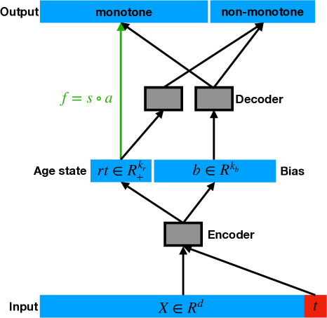
Figure G.4: The model structure. The features $X$ and age $t$ are fed into the encoder to approximate the posterior over the rates of aging $r$ and bias $b$. The grey boxes indicate functions parametrized by neural networks. While both the monotone and non-monotone outputs are a function of both the age state $rt$ and the bias $b$, only the relationship between $rt$ and the monotone outputs (green arrow) is constrained to be monotone and parametrized by $f=s\circ a$.

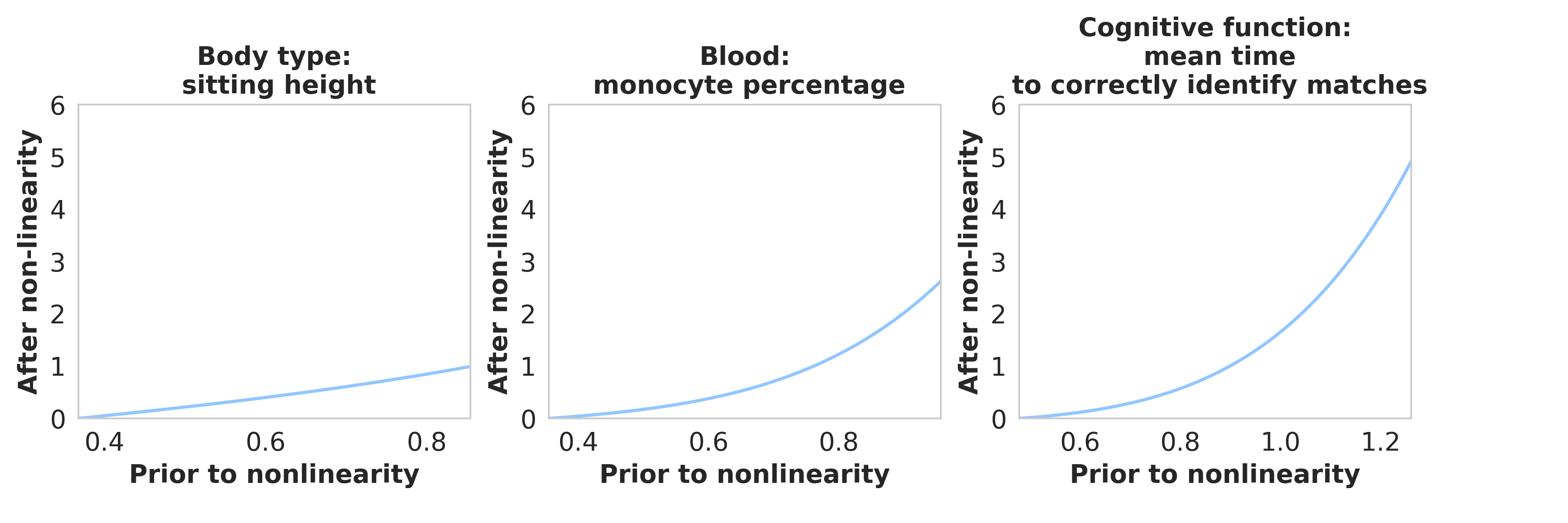
Figure G.5: Representative elementwise transformations $s$. Most elementwise transformations are close to linear, like the left plot, but some are not (right two plots). To determine the relevant domain for each elementwise transformation, we sample latent $rt$ from the fitted cross-sectional model (for $t$ = 40-69), feed it through the linear transformation $a$, and compute the 0.1th and 99.9th percentiles of the resulting distribution for each monotonic feature. This yields the relevant domain over which each elementwise transformation operates.

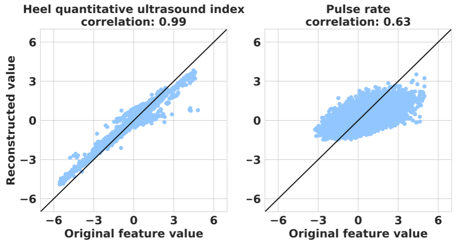
Figure G.6: Reconstructed vs. actual features. The figure plots the reconstructed $f(rt)+g(b)$ against the actual $x_{t}$ for the 2 features with the highest ($\rho=0.99$, left) and lowest correlation ($\rho=0.63$, right). Overall, the model fits the data well: reconstructed features are highly correlated with actual features (mean $\rho=0.88$), with most resembling the left plot.

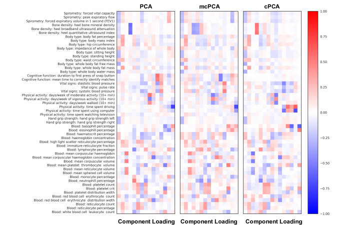
Figure G.7: Loadings for the three linear baselines (with 15 latent dimensions) reveal non-sparse latent dimensions which are difficult to interpret and do not clearly differentiate between age and non-age variation. Each cell shows the loading for one component (horizontal axis) and observed feature (vertical axis).

References

- Abid et al. [2018] A. Abid, M. J. Zhang, V. K. Bagaria, and J. Zou. Exploring patterns enriched in a dataset with contrastive principal component analysis. Nature Communications, 9(1), 2018.
- Äijö et al. [2014] T. Äijö, V. Butty, Z. Chen, V. Salo, S. Tripathi, C. B. Burge, R. Lahesmaa, and H. Lähdesmäki. Methods for time series analysis of RNA-seq data with application to human Th17 cell differentiation. Bioinformatics, 30(12), 2014.
- Bair et al. [2006] E. Bair, T. Hastie, D. Paul, and R. Tibshirani. Prediction by supervised principal components. Journal of the American Statistical Association (JASA), 101(473):119–137, 2006.
- Belsky et al. [2015] D. W. Belsky, A. Caspi, R. Houts, H. J. Cohen, D. L. Corcoran, A. Danese, H. Harrington, S. Israel, M. E. Levine, J. D. Schaefer, et al. Quantification of biological aging in young adults. Proceedings of the National Academy of Sciences, 112(30), 2015.
- Bendall et al. [2014] S. C. Bendall, K. L. Davis, E. D. Amir, M. D. Tadmor, E. F. Simonds, T. J. Chen, D. K. Shenfeld, G. P. Nolan, and D. Pe’er. Single-cell trajectory detection uncovers progression and regulatory coordination in human B cell development. Cell, 157(3):714–725, 2014.
- Bernstein and Sheldon [2016] G. Bernstein and D. Sheldon. Consistently estimating Markov chains with noisy aggregate data. In Artificial Intelligence and Statistics (AISTATS), pages 1142–1150, 2016.
- Borkan and Norris [1980] G. A. Borkan and A. H. Norris. Assessment of biological age using a profile of physical parameters. Journal of Gerontology, 35(2):177–184, 1980.
- Campbell and Yau [2017] K. Campbell and C. Yau. Uncovering genomic trajectories with heterogeneous genetic and environmental backgrounds across single-cells and populations. bioRxiv, 2017.
- Chen et al. [2016] B. H. Chen, R. E. Marioni, E. Colicino, M. J. Peters, C. K. Ward-Caviness, P. Tsai, N. S. Roetker, A. C. Just, E. W. Demerath, W. Guan, et al. DNA methylation-based measures of biological age: meta-analysis predicting time to death. Aging (Albany NY), 8(9), 2016.
- Collado [1997] M. D. Collado. Estimating dynamic models from time series of independent cross-sections. Journal of Econometrics, 82(1):37–62, 1997.
- Comfort [1969] A. Comfort. Test-battery to measure ageing-rate in man. The Lancet, 294(7635):1411–1415, 1969.
- Daniels and Velikova [2010] H. Daniels and M. Velikova. Monotone and partially monotone neural networks. IEEE Transactions on Neural Networks, 21(6):906–917, 2010.
- Di et al. [2009] C. Di, C. M. Crainiceanu, B. S. Caffo, and N. M. Punjabi. Multilevel functional principal component analysis. The Annals of Applied Statistics, 3(1), 2009.
- EuYu [2012] EuYu. A non-negative matrix has a non-negative inverse. What other properties does it have? https://math.stackexchange.com/q/214401, 2012.
- Fry et al. [2017] A. Fry, T. J. Littlejohns, C. Sudlow, N. Doherty, L. Adamska, T. Sprosen, R. Collins, and N. E. Allen. Comparison of sociodemographic and health-related characteristics of UK Biobank participants with those of the general population. American Journal of Epidemiology, 186(9):1026–1034, 2017.
- Furukawa et al. [1975] T. Furukawa, M. Inoue, F. Kajiya, H. Inada, S. Takasugi, S. Fukui, H. Takeda, and H. Abe. Assessment of biological age by multiple regression analysis. Journal of Gerontology, 30(4):422–434, 1975.
- Goodpaster et al. [2006] B. H. Goodpaster, S. W. Park, T. B. Harris, S. B. Kritchevsky, M. Nevitt, A. V. Schwartz, E. M. Simonsick, F. A. Tylavsky, M. Visser, and A. B. Newman. The loss of skeletal muscle strength, mass, and quality in older adults: the health, aging and body composition study. The Journals of Gerontology Series A: Biological Sciences and Medical Sciences, 61(10):1059–1064, 2006.
- Greven et al. [2011] S. Greven, C. Crainiceanu, B. Caffo, and D. Reich. Longitudinal functional principal component analysis. Recent Advances in Functional Data Analysis and Related Topics, 2011.
- Gupta and Bar-Joseph [2008] A. Gupta and Z. Bar-Joseph. Extracting dynamics from static cancer expression data. IEEE/ACM Transactions on Computational Biology and Bioinformatics (TCBB), 5(2):172–182, 2008.
- Gupta et al. [2016] M. Gupta, A. Cotter, J. Pfeifer, K. Voevodski, K. Canini, A. Mangylov, W. Moczydlowski, and A. V. Esbroeck. Monotonic calibrated interpolated look-up tables. Journal of Machine Learning Research (JMLR), 17(1):3790–3836, 2016.
- Hashimoto et al. [2016] T. Hashimoto, D. Gifford, and T. Jaakkola. Learning population-level diffusions with generative RNNs. In International Conference on Machine Learning (ICML), pages 2417–2426, 2016.
- Hawkins and Han [2000] D. Hawkins and C. Han. Estimating transition probabilities from aggregate samples plus partial transition data. Biometrics, 56(3):848–854, 2000.
- Hoffmann et al. [2015] J. J. Hoffmann, K. C. Nabbe, and N. M. van den Broek. Effect of age and gender on reference intervals of red blood cell distribution width (RDW) and mean red cell volume (MCV). Clinical Chemistry and Laboratory Medicine (CCLM), 53(12), 2015.
- Horvath [2013] S. Horvath. DNA methylation age of human tissues and cell types. Genome Biology, 14(10), 2013.
- Jang et al. [2017] E. Jang, S. Gu, and B. Poole. Categorical reparameterization with Gumbel-softmax. arXiv preprint arXiv:1611.01144, 2017.
- Jonsen et al. [2005] I. D. Jonsen, J. M. Flemming, and R. A. Myers. Robust state–space modeling of animal movement data. Ecology, 86(11):2874–2880, 2005.
- Kalbfleisch and Lawless [1984] J. D. Kalbfleisch and J. F. Lawless. Least-squares estimation of transition probabilities from aggregate data. Canadian Journal of Statistics, 12(3):169–182, 1984.
- King [2013] G. King. A Solution to the Ecological Inference Problem: Reconstructing Individual Behavior from Aggregate Data. Princeton University Press, 2013.
- Kingma and Ba [2014] D. Kingma and J. Ba. Adam: A method for stochastic optimization. arXiv preprint arXiv:1412.6980, 2014.
- Kingma and Welling [2014] D. P. Kingma and M. Welling. Auto-encoding variational Bayes. arXiv preprint arXiv:1312.6114, 2014.
- Klemera and Doubal [2006] P. Klemera and S. Doubal. A new approach to the concept and computation of biological age. Mechanisms of Ageing and Development, 127(3):240–248, 2006.
- Kraemer et al. [2000] H. C. Kraemer, J. A. Yesavage, J. L. Taylor, and D. Kupfer. How can we learn about developmental processes from cross-sectional studies, or can we? American Journal of Psychiatry, 157(2):163–171, 2000.
- Kumar et al. [2017] P. Kumar, Y. Tan, and P. Cahan. Understanding development and stem cells using single cell-based analyses of gene expression. Development, 144(1):17–32, 2017.
- Lane et al. [2016] J. M. Lane, I. Vlasac, S. G. Anderson, S. D. Kyle, W. G. Dixon, D. A. Bechtold, S. Gill, M. A. Little, A. Luik, A. Loudon, et al. Genome-wide association analysis identifies novel loci for chronotype in 100,420 individuals from the UK biobank. Nature Communications, 7, 2016.
- Levine [2012] M. E. Levine. Modeling the rate of senescence: can estimated biological age predict mortality more accurately than chronological age? Journals of Gerontology Series A: Biomedical Sciences and Medical Sciences, 68(6):667–674, 2012.
- Louis et al. [1986] T. A. Louis, J. Robins, D. W. Dockery, A. Spiro, and J. H. Ware. Explaining discrepancies between longitudinal and cross-sectional models. Journal of Clinical Epidemiology, 39(10):831–839, 1986.
- MacDonald et al. [2004] S. W. MacDonald, R. A. Dixon, A. Cohen, and J. E. Hazlitt. Biological age and 12-year cognitive change in older adults: findings from the victoria longitudinal study. Gerontology, 50(2):64–81, 2004.
- Maddison et al. [2016] C. J. Maddison, A. Mnih, and Y. W. Teh. The concrete distribution: A continuous relaxation of discrete random variables. arXiv preprint arXiv:1611.00712, 2016.
- Magwene et al. [2003] P. M. Magwene, P. Lizardi, and J. Kim. Reconstructing the temporal ordering of biological samples using microarray data. Bioinformatics, 19(7):842–850, 2003.
- McClearn [1997] G. E. McClearn. Biogerontologic theories. Experimental Gerontology, 32(1):3–10, 1997.
- Milovanovic et al. [2004] M. Milovanovic, E. Nilsson, and P. Järemo. Relationships between platelets and inflammatory markers in rheumatoid arthritis. Clinica Chimica Acta, 343(1):237–240, 2004.
- Moffitt [1993] R. Moffitt. Identification and estimation of dynamic models with a time series of repeated cross-sections. Journal of Econometrics, 59(1):99–123, 1993.
- Mozaffarian et al. [2011] D. Mozaffarian, T. Hao, E. B. Rimm, W. C. Willett, and F. B. Hu. Changes in diet and lifestyle and long-term weight gain in women and men. New England Journal of Medicine, 364(25):2392–2404, 2011.
- Nakamura et al. [1988] E. Nakamura, K. Miyao, and T. Ozeki. Assessment of biological age by principal component analysis. Mechanisms of Ageing and Development, 46(1):1–18, 1988.
- Nowell [1976] P. C. Nowell. The clonal evolution of tumor cell populations. Science, 194(4260):23–28, 1976.
- O’Reilly et al. [2012] P. F. O’Reilly, C. J. Hoggart, Y. Pomyen, F. C. Calboli, P. Elliott, M. Jarvelin, and L. J. Coin. MultiPhen: joint model of multiple phenotypes can increase discovery in GWAS. PloS One, 7(5), 2012.
- Plas [1983] A. P. V. D. Plas. On the estimation of the parameters of Markov probability models using macro data. Annals of Statistics, 1:78–85, 1983.
- Putin et al. [2016] E. Putin, P. Mamoshina, A. Aliper, M. Korzinkin, A. Moskalev, A. Kolosov, A. Ostrovskiy, C. Cantor, J. Vijg, and A. Zhavoronkov. Deep biomarkers of human aging: application of deep neural networks to biomarker development. Aging, 8(5), 2016.
- Qiu et al. [2011] P. Qiu, A. J. Gentles, and S. K. Plevritis. Discovering biological progression underlying microarray samples. PLoS Computational Biology, 7(4), 2011.
- Qu and Hu [2011] Y. Qu and B. Hu. Generalized constraint neural network regression model subject to linear priors. IEEE Transactions on Neural Networks, 22(12):2447–2459, 2011.
- Ram [1986] R. Ram. Government size and economic growth: A new framework and some evidence from cross-section and time-series data. The American Economic Review, 76(1):191–203, 1986.
- Reid and Wernisch [2016] J. E. Reid and L. Wernisch. Pseudotime estimation: deconfounding single cell time series. Bioinformatics, 32(19):2973–2980, 2016.
- Relethford et al. [1978] J. H. Relethford, F. C. Lees, and P. J. Byard. The use of principal components in the analysis of cross-sectional growth data. Human Biology, pages 461–475, 1978.
- Rossol et al. [2012] M. Rossol, S. Kraus, M. Pierer, C. Baerwald, and U. Wagner. The CD14brightCD16+ monocyte subset is expanded in rheumatoid arthritis and promotes expansion of the Th17 cell population. Arthritis & Rheumatology, 64(3):671–677, 2012.
- Stanojevic et al. [2008] S. Stanojevic, A. Wade, J. Stocks, J. Hankinson, A. L. Coates, H. Pan, M. Rosenthal, M. Corey, P. Lebecque, and T. J. Cole. Reference ranges for spirometry across all ages: a new approach. American Journal of Respiratory and Critical Care Medicine, 177(3):253–260, 2008.
- Stein and Shakarchi [2011] E. M. Stein and R. Shakarchi. Fourier Analysis: an Introduction, volume 1. Princeton University Press, 2011.
- Sudlow et al. [2015] C. Sudlow, J. Gallacher, N. Allen, V. Beral, P. Burton, J. Danesh, P. Downey, P. Elliott, J. Green, M. Landray, et al. UK Biobank: an open access resource for identifying the causes of a wide range of complex diseases of middle and old age. PLoS Medicine, 12(3), 2015.
- Trapnell et al. [2014] C. Trapnell, D. Cacchiarelli, J. Grimsby, P. Pokharel, S. Li, M. Morse, N. J. Lennon, K. J. Livak, T. S. Mikkelsen, and J. L. Rinn. The dynamics and regulators of cell fate decisions are revealed by pseudotemporal ordering of single cells. Nature Biotechnology, 32(4), 2014.
- Waddington [1940] C. H. Waddington. Organisers and Genes. University Press; Cambridge, 1940.
- Wain et al. [2015] L. V. Wain, N. Shrine, S. Miller, V. E. Jackson, I. Ntalla, M. S. Artigas, C. K. Billington, A. K. Kheirallah, R. Allen, J. P. Cook, et al. Novel insights into the genetics of smoking behaviour, lung function, and chronic obstructive pulmonary disease (UK Bileve): a genetic association study in UK Biobank. The Lancet Respiratory Medicine, 3(10):769–781, 2015.
- Wang et al. [2018] Y. Wang, B. Dai, L. Kong, X. Ma, S. M. Erfani, J. Bailey, S. Xia, L. Song, and H. Zha. Learning deep hidden nonlinear dynamics from aggregate data. In Uncertainty in Artificial Intelligence (UAI), 2018.
- You et al. [2017] S. You, D. Ding, K. Canini, J. Pfeifer, and M. Gupta. Deep lattice networks and partial monotonic functions. In Advances in Neural Information Processing Systems (NeurIPS), pages 2985–2993, 2017.