Group Invariance and Computational Sufficiency

Abstract

Statistical sufficiency formalizes the notion of data reduction. In the decision theoretic interpretation, once a model is chosen all inferences should be based on a sufficient statistic. However, suppose we start with a set of procedures rather than a specific model. Is it possible to reduce the data and yet still be able to compute all of the procedures? In other words, what functions of the data contain all of the information sufficient for computing these procedures? This article presents some progress towards a theory of “computational sufficiency” and shows that strong reductions can be made for large classes of penalized $M$-estimators by exploiting hidden symmetries in the underlying optimization problems. These reductions can (1) reveal hidden connections between seemingly disparate methods, (2) enable efficient computation, (3) give a different perspective on understanding procedures in a model-free setting. As a main example, the theory provides a surprising answer to the following question: “What do the Graphical Lasso, sparse PCA, single-linkage clustering, and L1 penalized Ising model selection all have in common?”

1 Introduction

The extraction of information and the reduction of data are central concerns of statistics. One formalization of these notions is the concept of statistical sufficiency introduced by [10] in his seminal article “On the Mathematical Foundations of Theoretical Statistics”:

“A statistic satisfies the criterion of sufficiency when no other statistic which can be calculated from the same sample provides any additional information as to the value of the parameter to be estimated.”

Implicit in Fisher’s definition is the specification of a statistical model and the sense in which a sufficient statistic “contains all of the information in the sample.” In the decision theoretic interpretation, once a model is specified all inferences should (or might as well) be based on a sufficient statistic—for any procedure based on the data there is an equivalent randomized procedure based on a sufficient statistic [15, see, e.g.,]. However, actual data analysis does not always begin with the specification of a model, and it may not even make explicit use of a statistical model. [4] famously described two cultural perspectives on data analysis:

“One assumes that the data are generated by a given stochastic data model. The other uses algorithmic models and treats the data mechanism as unknown.”

In the former case, the statistical model gives context to “information” and statistical sufficiency can be seen as a criterion for separating the “relevant information” from the “irrelevant information.” In the latter case, a statistical model is absent and statistical sufficiency is of no use. Rather than positing a collection of probability distributions (a statistical model), the data analyst might instead consider a collection of procedures or algorithms. So how should we formalize data reduction and what is the proper context for defining “relevant information” from an algorithmic perspective? This article proposes a concept called computational sufficiency.

Computational sufficiency defines information in the context of a collection of procedures that share a common input domain. It is motivated in part by the following questions.

1. Are there hidden commonalities between the procedures?

2. Are there parts of the data that are irrelevant to all of the procedures?

3. Can we reduce the data by removing the irrelevant parts?

4. Can we exploit this reduction for computation?

5. What is the most relevant core of the data?

Precise definitions will be given in Section 3, but the basic idea is simple: a statistic (or reduction) is computationally sufficient if every procedure in the collection is essentially a function of the statistic. The data itself is computationally sufficient, because every procedure is already a function of the data. So the definition is only really useful if there are nontrivial reductions. The main point of this article is to show that nontrivial reductions do exist for large classes of procedures, and that by studying reductions within the framework of computational sufficiency, interesting and insightful answers can be made to the above questions. This provides a different perspective on understanding data analysis procedures when a statistical model may not be present.

The article proceeds in a manner roughly paralleling the author’s own process of discovery. Section 2 presents the main motivating example, where a commonality between three seemingly disparate methods is demonstrated empirically on a real dataset. The connection between two of those is already known and discussed in Section 2.3, but what is surprising (at least to me) is that the phenomenon generalizes to a large classes of procedures. Section 3 gives precise definitions for computational sufficiency and related concepts, and attempts to explain the parallels and differences with statistical sufficiency. The section also begins the main arc of the paper, which is a theoretical framework for the construction of computationally sufficient reductions. This includes defining a class of procedures that generalize penalized maximum likelihood for exponential families (Section 4). Within this class, the primary mathematical tool for finding commonalities is the exploitation of symmetries via group invariance (Section 5). This allows us, in Section 6, to construct nontrivial reductions that are computationally sufficient, and to return to the main example in Section 7 with deeper insight. Additional extensions and discussion are given in Section 8.

2 A motivating example

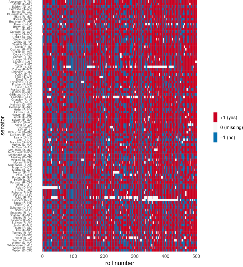
Figure 1: Senate roll call votes from the 114^th U.S. Congress. Each row is the voting record of a senator, arranged from earliest (left) to latest (right). Horizontal white stripes indicate consecutively missed votes. The longest of these correspond to senators who campaigned for the 2016 U.S. Presidential election.

Political polarization is a defining feature of 21^st century American politics [22]. One manifestation of this is in the clustering of voting patterns of political representatives in the United States government. Figure 1 displays $n=502$ senate roll call votes from the 114^th United States Congress (January, 2015 – January, 2017) for each of the $p=100$ senators. The votes are coded numerically as $+1$ for “yes”, $-1$ for “no”, and $0$ if the vote was missed.

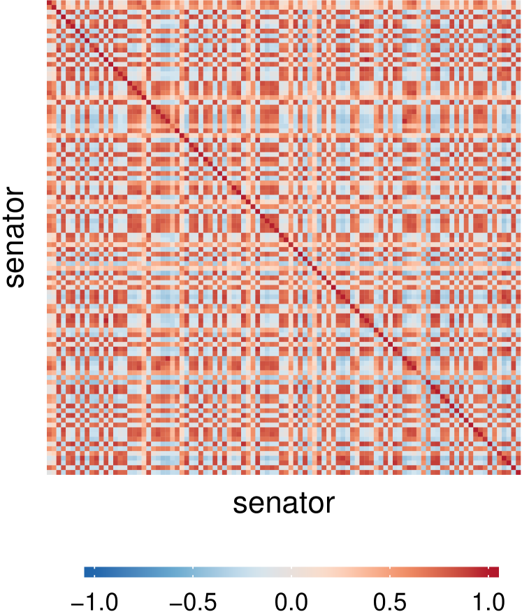
(a) Sorted by name

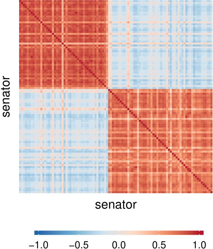
(b) Sorted by political party

Figure 2: The sample covariance matrix of senators’ roll call votes. Positive entries indicate relative agreement, while negative entries indicate relative disagreement. (2(a)) Senators sorted by name. (2(b)) Senators sorted by political party affiliation (Democrat, Independent, or Republican) with ties broken by name. The two diagonal blocks correspond to Democrats (upper-left) and Republicans (lower-right). Two Independent senators are placed in the middle at positions 45–46; they essentially vote with the Democrats.

Relative agreement or disagreement between voting patterns of pairs of senators can be summarized by taking the average of the product of the entries of their corresponding vectors, i.e. we form a matrix $X\in\mathbb{R}^{p\times p}$ with entries

$$x_{ij}=\frac{1}{n}\sum_{t=1}^{n}v_{ti}v_{tj}=\frac{(\text{\# of agreements})-(\text{\# of disagreements})}{n}\,,$$ (2.1)

where $v_{ti}$ is the vote of senator $i$ on roll call $t$. This can be viewed as an uncentered sample covariance: it is positive when the pair of senators tend to vote together, and it is negative when they tend to vote against each other. The resulting matrix $X$ is displayed in Figure 2. There is no easily discernible pattern when the senators are sorted alphabetically by name (Figure 2(a)), but when sorted by political party affiliation—all but 2 senators are affiliated with either the Republican Party or Democrat Party—a clear pattern emerges: the voting pattern of the senators appears to cluster according to political party (Figure 2(b)).

2.1 Single-linkage cluster analysis

(a) Single-linkage dendrogram

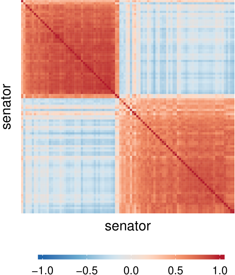
(b) Sample covariance matrix sorted by single-linkage

Figure 3: Single-linkage clustering applied to the roll call vote data with similarity measure $\lvert x_{ij}\rvert$, i.e. magnitude of the sample covariance. (3(a)) The leaves of the dendrogram are labeled by political party affiliation. Note that the value of $\lambda$ decreases with increasing height in the tree. The main right branch of the tree consists only of Republicans, while the left branch contains all of the Democrats and two Independents. (3(b)) The sample covariance matrix is sorted according to the left-to-right ordering of leaves in the single-linkage dendrogram. The two diagonal blocks again correspond to Democrats (upper-left) and Republicans (lower-right). Two independent senators are mixed together with the Democrats.

To contrast with the nominal clustering provided by political party affiliation, the data analyst might instead employ an intrinsic cluster analysis using the roll call votes alone. One well-known technique is single-linkage clustering [39], which is a hierarchical clustering procedure that takes a similarity measure as input. The algorithm starts from the finest clustering, where each senator is placed in his/her own cluster, and iteratively merges the most similar pairs of clusters until a single cluster remains. The similarity between a pair of clusters is defined to be the maximum of the pairwise similarities between their respective constituents, so with each merge there is always a “single link” that binds the clusters together. The results of the process are encoded in a dendrogram: a tree whose leaves are senators and internal vertices are merges. The height of a vertex corresponds to the similarity between a pair of clusters just before merging. Cutting the dendrogram at different heights induces different, but hierarchically arranged, clusterings. (See Appendix A for a graph-theoretic description of single-linkage.)

Figure 3 shows the result of single-linkage clustering applied to the roll call data with similarity measure $\lvert x_{ij}\rvert$. Though the choice of absolute sample covariance may seem odd, the rationale for this choice will become clear later. Looking at the dendrogram (Figure 3(a)), we see that the large gap between the merge heights of the Democrats (in the left branch of the dendrogram) and the Republicans (in the right branch of the dendrogram) reflects the polarization of their voting patterns. Comparing the sample covariance matrix sorted by political party (Figure 2(b)) and by single-linkage (Figure 3(b)), we see that single-linkage not only recovers the party affiliation, but the relative smoothness of the gradients of diagonal blocks suggests that single-linkage may have also discovered some finer structure in the data.

2.2 Sparse multivariate methods

Continuing with a progression of technique, the data analyst may find himself enticed by more recent and potentially more powerful multivariate methods employing sparsity. Two such methods are sparse inverse covariance estimation and sparse principal components analysis (or sparse PCA). [17, Chapters 8.2 and 9 ] give an excellent overview and bibliographic notes. These methods can be viewed as sparse estimators of functionals of a population covariance matrix $\Sigma$. In one case, the functional is simply the inverse $\Sigma^{-1}$, while for PCA the functional is the projection matrix of the subspace spanned by the $k$ leading eigenvectors (or principal component directions). There are many different formulations of these methods; here we consider two formulations based on convex programming: Graphical Lasso  [51, 12, 1] and Sparse PCA via Fantope Projection [6, 45].

Graphical Lasso is a penalized maximum likelihood method based on the convex optimization problem,

minimize $$-\log\det(\theta)+\langle X,\theta\rangle+\lambda\lVert\theta\rVert_{1}\,,$$ (2.2)

where $\langle,\rangle$ denotes the trace inner product, $\lambda\geq 0$ is a tuning parameter, and $\lVert\>\cdot\>\rVert_{1}$ is the $\ell_{1}$ norm–the sum of the absolute values of the coordinates of its argument. 2.2 is a penalized Gaussian log-likelihood. The $\ell_{1}$ penalty encourages sparsity in the solution, with larger values of $\lambda$ yielding solutions with more zero entries. If $\theta$ is the inverse covariance matrix of a multivariate Gaussian distribution, then the interpretation is that $\theta_{ij}$ is $0$ if and only if variables $i$ and $j$ are conditionally independent, given the other variables.

Sparse PCA via Fantope Projection is also based on convex optimization, but more specifically, it is based the semidefinite optimization problem,

maximize $$\langle X,\theta\rangle-\lambda\lVert\theta\rVert_{1}$$ (2.3)

subject to $$\theta\in\mathcal{F}^{k}\,,$$

where

$$\mathcal{F}^{k}\coloneqq\{\theta\nonscript\>|\allowbreak\nonscript\>\mathopen{}0\preceq\theta\preceq I,\operatorname{trace}(\theta)=k\}\,.$$ (2.4)

This can be viewed as an $\ell_{1}$ penalized convex relaxation of the variance maximization problem. The constraint set $\mathcal{F}^{k}$ consists of symmetric matrices with eigenvalues between $0$ and $1$ and whose trace is equal to $k$. This is called the Fantope and it is the convex hull of rank-$k$ projection matrices [45]. The interpretation of $\lambda$ and the $\ell_{1}$ penalty are similar to the Graphical Lasso—they influence the sparsity of the solution. Sparsity of a projection implies that the principal components depend on a small number of variables. There is, however, an additional user-chosen parameter $k$ that specifies the desired rank of estimated projection matrix and hence the number of principal components.

(a) Single-linkage clustering

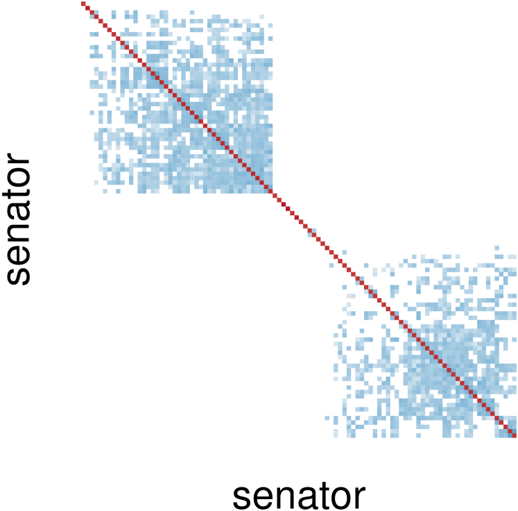
(b) Graphical Lasso

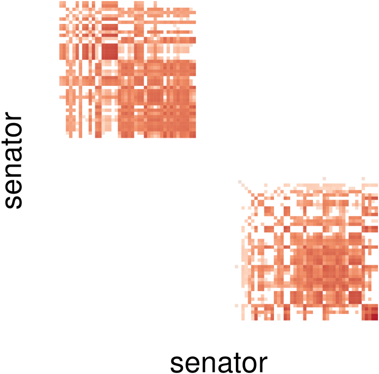
(c) Sparse PCA via Fantope Projection

Figure 4: (4(a)) The single-linkage clustering matrix and estimates of the (4(b)) inverse covariance matrix and (4(c)) principal components projection matrix. These are all based on the senator-senator sample covariance matrix, and in all three cases the tuning parameters and dendrogram cut height are set to $\lambda=0.7$.

Figure 4 shows the results of Graphical Lasso and Sparse PCA via Fantope Projection applied to the senator-senator sample covariance matrix 2.1. The tuning parameter for both procedures was set to $\lambda=0.7$ and $k=5$ was chosen for Sparse PCA. Figure 4(a) shows the result of cutting single-linkage dendrogram at $\lambda=0.7$ as a clustering matrix—a binary matrix with $1$ in entry $i,j$ if and only if $i$ and $j$ are in the same cluster. Remarkably, the block-diagonal structure is very similar across all three methods, and all three methods capture large chunks of the two major political parties. In fact, the supports of both the Graphical Lasso and Sparse PCA estimates are contained in the support of the single-linkage clustering matrix, and this continues to hold for other choices of $\lambda$. One possible summary of this phenomenon is that the Graphical Lasso and Sparse PCA seem to be refinements of single-linkage. While single-linkage easily discovers the two big blocks, the more sophisticated techniques reveal finer structure within the blocks.

2.3 Exact thresholding, the Graphical Lasso, and more

The similarity between Graphical Lasso and single-linkage clustering shown in Figure 4 is an instance of the “exact thresholding” phenomenon first observed by [31, 48]. In brief, they proved that the graph formed by thresholding the entries of $X$ at level $\lambda$—by setting to zero any entry with $\lvert x_{ij}\rvert\leq\lambda$—and the estimated inverse covariance graph produced by the Graphical Lasso with tuning parameter $\lambda$ have exactly the same connected components. In other words, the thresholded matrix $X$ and the Graphical Lasso estimate have exactly the same block-diagonal structure. The proofs of [31, 48] are similar; they are based on direct examination of the Karush–Kuhn–Tucker (KKT) optimality conditions for 2.2 and exploit special properties of the log-determinant. Building on the exact thresholding phenomenon, [41] later observed that the connected components of the Graphical Lasso correspond to the clusters of single-linkage with similarity measure $\lvert x_{ij}\rvert$.

The connection between exact thresholding, the Graphical Lasso, and single-linkage clustering has several implications, and two perspectives have emerged in the literature: algorithmic and methodological. [48, 31] showed that exact thresholding leads to faster algorithms for the Graphical Lasso. For a $p\times p$ input $X$, generic solvers for the Graphical Lasso optimization problem 2.2 have $O(p^{3})$ time complexity per iteration. On the other hand, thresholding and identifying the connected components has worst case time complexity $O(p^{2})$. Once the connected components are identified, the parameter space, i.e. the feasible set, of the optimization problem can be reduced and decomposed to smaller, separate blocks. This reduces the Graphical Lasso optimization problem into separate smaller problems that can be solved in parallel and more quickly than the original problem. This algorithmic aspect of phenomenon has been extended on a case-by-case basis to various generalizations of the Graphical Lasso [5, 32, 34, 40, 53].

On the methodological side, [14] used the monotonicity property implied by the exact thresholding phenomenon to develop adaptive sequential hypothesis tests based on examining “knots” in the Graphical Lasso solution path—these knots correspond to the merge events in single-linkage. [41] took a critical perspective by using the connection to motivate alternative estimators of the inverse covariance matrix. They noted that Graphical Lasso could be viewed as a two-step procedure. In the first step, it performs single-linkage clustering with similarity measure $\lvert x_{ij}\rvert$. In the second step, it performs penalized maximum likelihood estimation on each connected component. Focusing on the first step, they argue that single-linkage clustering has an undesirable “chaining” effect [16, see, e.g.,], and propose to replace it with an alternative clustering algorithm. They call the resulting two-step estimator “Cluster Graphical Lasso,” and demonstrate empirically some of its advantages over the Graphical Lasso.

The implications of exact thresholding discussed above add insight to our collective understanding of the Graphical Lasso. Recalling the questions posed in the introduction, we see that the exact thresholding phenomenon explains that there are hidden commonalities between single-linkage clustering and the Graphical Lasso, and that this can be exploited for reduction in computation. Yet there is much more to the phenomenon. In Section 7, we will see that not only can the parameter space of the Graphical Lasso problem be reduced, but that the input $X$ to the Graphical Lasso optimization problem can essentially be replaced by $\operatorname{SLT}_{\lambda}(X)$, the single-linkage thresholding operator:

$$[\operatorname{SLT}_{\lambda}(X)]_{ij}=\begin{cases}x_{ij}&\text{ if $i\sim_{\lambda}j$, and}\\ 0&\text{otherwise,}\end{cases}$$

where $i\sim_{\lambda}j$ means that $i$ and $j$ are in the same single-linkage cluster at level $\leq\lambda$. This will demonstrate that there are irrelevant parts of the data that can be removed, and perhaps more surprisingly, Sections 6 and 7 will show that this type of phenomenon extends beyond the Graphical Lasso and holds simultaneously for many other procedures.

3 Computational sufficiency

Given a collection of procedures that share a common input domain $\mathcal{X}$, we would like to be able to reduce the input and yet still be able to compute each procedure. So our goal is to define concepts that identify the information that is sufficient and necessary for computing all of the procedures. Some of the procedures considered in Section 2 are based on optimization. Such estimators may not always be uniquely defined and they may not even exist for some inputs. For example, optimization problem 2.3 may have more than one solution, and 2.2 may not even have a solution if $\lambda=0$. With these complications in mind, we define a procedure to be a set-valued function on $\mathcal{X}$. For example, let $T(x)$ denote the set of solutions of 2.3 when $X=x$. Then every element of $T(x)$ achieves the same value of the objective function. Defining a procedure to be a set-valued function provides a convenient way to describe equivalent and/or possibly void results.

3.1 Definitions

Let $\mathcal{M}$ be a collection of set-valued functions on $\mathcal{X}$. This is our collection of procedures. The effective domain of a set-valued function $T$ is defined to be

$$\operatorname{dom}T\coloneqq\{x\in\mathcal{X}\nonscript\>|\allowbreak\nonscript\>\mathopen{}T(x)\neq\emptyset\}\,.$$

If the data analyst is content to obtain any singleton from $T(x)$, whenever $x\in\operatorname{dom}T$, then

Definition 1.

A function $R$ on $\mathcal{X}$ is computationally sufficient for $\mathcal{M}$ if for each $T\in\mathcal{M}$, there exists a set-valued function $f$ such that $f(T,R(x))\neq\emptyset$ for all $x\in\operatorname{dom}T$ and

$$f(T,R(x))\subseteq T(x)\quad\text{for all}\quad x\in\mathcal{X}\,.$$ (3.1)

When this is the case, we may refer to $R$ as being a reduction.

Criterion 3.1 says that every $T\in\mathcal{M}$ is essentially a function of $R$—up to the equivalence implied by the set-valuedness of $T$. If $T$ is singleton-valued, then 3.1 becomes an equality. The identity map is trivially computationally sufficient, but clearly provides no reduction. So in the pursuit of reduction without loss of information, there is an obvious interest in finding a maximal reduction. The following definitions parallel the definitions of necessary and minimal sufficient statistics.

Definition 2.

A function $U$ is computationally necessary for $\mathcal{M}$ if for each $R$ that is computationally sufficient for $\mathcal{M}$, there exists $h$ such that

$$U(x)=h(R(x))\quad\text{for all}\quad x\in\mathcal{X}\,.$$

If $U$ is computationally necessary and computationally sufficient, then we say that $U$ is computationally minimal.

By definition, every singleton-valued $T\in\mathcal{M}$ is computationally necessary for $\mathcal{M}$. This simple observation leads to the following result and needs no proof.

Lemma 1.

If $R\in\mathcal{M}$ is singleton-valued and computationally sufficient for $\mathcal{M}$, then $R$ is computationally minimal.

This seemingly trivial statement will turn out to be a useful device for establishing computational minimality. An immediate consequence is that if any $T\in\mathcal{M}$ is a bijection, then the identity map is computationally minimal and no further reduction is possible. So in order for a nontrivial reduction to exist, it is necessary that all of the procedures in $\mathcal{M}$ be noninvertible.

3.2 Reductions and partitions

Nontrivial computationally sufficient reductions are only possible when the procedures under consideration are themselves nontrivial reductions. Heuristically, this means that the preimages of the results of different procedures should be large and coincide with one another. If every $T\in\mathcal{M}$ is singleton-valued, then the criterion of computational sufficiency can be expressed more simply as

$$T(x)=f(T,R(x))\quad\text{for all}\quad x\in\operatorname{dom}T\,.$$ (3.2)

When this is the case, computational sufficiency can be stated in terms of the partitions of $\mathcal{X}$. For a function $h$ on $\mathcal{X}$, let

$$\sigma(h)\coloneqq\bigcup_{x\in\mathcal{X}}\big{\{}\{u\nonscript\>|\allowbreak\nonscript\>\mathopen{}T(u)=T(x)\}\}\,,$$

i.e. $\sigma(h)$ is the the partition of $\mathcal{X}$ induced by $h$. We can order the set of all partitions of $\mathcal{X}$ by refinement, writing $\alpha\preceq\beta$ if $\alpha$ refines $\beta$. Then $R$ is computationally sufficient for $\mathcal{M}$ if and only if

$$\sigma(R)\preceq\sigma(T)\quad\text{for all}\quad T\in\mathcal{M}\,.$$

A function $U$ on $\mathcal{X}$ is computationally necessary for $\mathcal{M}$ if and only if

$$\sigma(R)\preceq\sigma(U)$$

for all computationally sufficient $R$. Since ordering by refinement turns the set of all partitions of $\mathcal{X}$ into a complete lattice, there exists a coarsest partition that refines all of the partitions $\sigma(T)$ induced by $T\in\mathcal{M}$. That greatest lower bound is the partition induced by a computationally minimal reduction for $\mathcal{M}$. This description of computational sufficiency in terms of partitions is conceptually useful, but it seems practically impossible to reason about specific procedures in terms of the partitions that they induce.

3.3 Computational sufficiency versus statistical sufficiency

Expression 3.2 bears a strong resemblance to the factorization criterion of the Fisher–Neyman Theorem for statistical sufficiency. Suppose that $\mathcal{P}$ is a family of positive densities on $\mathcal{X}$. Then a statistic $R$ is sufficient for $\mathcal{P}$ if and only if there exist $g$ and $h$ such that for all $q\in\mathcal{P}$

$$q(x)=g(q,R(x))h(x)\quad\text{for all}\quad x\in\mathcal{X}\,.$$

Fixing any $q_{0}\in\mathcal{P}$ and dividing both sides, the above criterion is equivalent to the existence of $f$ such that for all $q\in\mathcal{P}$,

$$\frac{q(x)}{q_{0}(x)}=f(q/q_{0},R(x))\quad\text{for all}\quad x\in\mathcal{X}$$

[15, c.f.]. Letting $\mathcal{Q}=\{q/q_{0}\nonscript\>|\allowbreak\nonscript\>\mathopen{}q\in\mathcal{P}\}$ we see immediately that there is a clear computational interpretation of statistical sufficiency: $R$ is statistically sufficient for $\mathcal{P}$ if and only if it is computationally sufficient for the likelihood ratios $q/q_{0}$. The connection goes further. The following result is a straightforward consequence of definitions.

Lemma 2.

Let $\Lambda$ be a function on $\mathcal{X}$ with values taking the form of a function on $\mathcal{M}$. For each $x\in\mathcal{X}$ define

$$\lparen\Lambda(x)\rparen(T)=T(x)\quad\text{for all}\quad T\in\mathcal{M}.$$

Then $\Lambda$ is computationally minimal for $\mathcal{M}$.

Applying this to $\mathcal{Q}$, we see that that the likelihood ratios are computationally minimal, and hence statistically sufficient. We can also deduce that they are statistically minimal sufficient.

One way to view the philosophical difference between computational sufficiency and statistical sufficiency is that definition of statistical sufficiency starts from conditional probability and is in essence about isolating the information that is sufficient for computing conditional expectation for any distribution in the model. In the measure-theoretic setting this, unfortunately, entails substantial technical complications that preclude the conclusion of the Fisher–Neyman factorization theorem from always being true. Computational sufficiency, on the other hand, starts from a definition that is analogous to the factorization criterion, and that directly isolates the information that is sufficient for computing either the procedures or the likelihood.

4 Expofam-type estimators

To demonstrate the general existence and feasibility of computationally sufficient reductions we introduce a framework for procedures that are generalizations of penalized maximum likelihood for exponential family models. Let $\mathcal{X}$ be a Euclidean space equipped with an inner product $\langle,\rangle$ which induces a norm $\lVert\>\cdot\>\rVert$. We say that a set-valued function $T$ on $\mathcal{X}$ is an expofam-type estimator if it has the form

$$T(x)=\operatornamewithlimits{arg\,min}_{\theta}A(\theta)-\langle x,\theta\rangle+h_{C}(\theta)\,,$$ (4.1)

where $A:\mathcal{X}\to\mathbb{R}\cup\{+\infty\}$ is the called the generator of $T$ and and $h_{C}:\mathcal{X}\to\mathbb{R}\cup\{+\infty\}$ is the support function,

$$h_{C}(\theta)=\max_{z\in C}\langle z,\theta\rangle\,,$$

of a nonempty, closed and convex set $C$. We will assume that $A$ is closed (lower semicontinuous), convex and proper (finite for at least one value in $\mathcal{X}$). The optimization problem in 4.1 may possibly have multiple or no solutions depending on $x$, so it is important that we view $T$ as being a set-valued function on $\mathcal{X}$.

There are several important features of this formulation. The objective function in 4.1 should be viewed as being the sum of two parts: a loss, $A(\theta)-\langle x,\theta\rangle$, and a penalty, $h_{C}(\theta)$. Both parts are closed convex functions and so their sum is also a closed convex function. The loss strictly generalizes the negative log-likelihood of an exponential family. We only require that $A$ be a closed, convex and proper function, so in general it may not be the log-partition function of an exponential family of distributions. The penalty generalizes seminorms, and in fact any closed sublinear function can be viewed as the support function of some closed convex set [18, e.g.]. The importance of viewing the penalty in this way is that it establishes a link between functions and sets.

Many existing procedures fit into the framework of 4.1, and it is useful to organize them according to their generator $A$ and penalty support set $C$. Tables 1 and 2 gives some examples. There are numerous others, but our main focus in this article will be on the examples that follow.

Method	$A(\theta)$
Least squares	$\frac{1}{2}\lVert\theta\rVert^{2}$
Constrained least squares	$\frac{1}{2}\lVert\theta\rVert^{2}+\iota_{K}(\theta)$
Inverse covariance	$-\log\det(-\theta)$
PCA	$\iota_{\mathcal{F}^{k}}(\theta)$
Ising model	$\log\sum_{u\in\{-1,+1\}^{p}}\exp(\langle uu^{T},\theta\rangle)$

Table 1: Examples of generators $A$

Penalty	$C$
Lasso ($\ell_{1}$)	$\{z\nonscript\>|\allowbreak\nonscript\>\mathopen{}\lVert z\rVert_{\infty}\leq\lambda\}$
Group Lasso ($\ell_{1,2}$)	$\{z\nonscript\>|\allowbreak\nonscript\>\mathopen{}\max_{i}\lVert z_{i}\rVert\leq\lambda\}$
General norms ($\nu$)	$\{z\nonscript\>|\allowbreak\nonscript\>\mathopen{}\nu_{*}(z)\leq\lambda\}$
Cone constraint ($\iota_{K}$)	$K^{\circ}=\{z\nonscript\>|\allowbreak\nonscript\>\mathopen{}h_{K}(z)\leq 0\}$

Table 2: Examples of penalty support sets $C$

4.1 Penalized least squares with constraints

The most basic example is obtained by taking

$$A(\theta)=\frac{1}{2}\lVert\theta\rVert^{2}\,,$$

so that 4.1 becomes equivalent to penalized least squares:

$$T(x)=\operatornamewithlimits{arg\,min}_{\theta}\frac{1}{2}\lVert x-\theta\rVert^{2}+h_{C}(\theta)\,.$$

Sometimes it can be useful to put constraints on $\theta$, say $\theta\in K$ for some closed convex set $K$. We can incorporate this constraint into $A$ by adding the convex indicator function

$$\iota_{K}(\theta)=\begin{cases}0&\text{if $\theta\in K$, and}\\ +\infty&\text{otherwise.}\end{cases}$$

Then with

$$A(\theta)=\frac{1}{2}\lVert\theta\rVert^{2}+\iota_{K}(\theta)\,,$$

4.1 becomes

$$T(x)=\operatornamewithlimits{arg\,min}_{\theta\in K}\frac{1}{2}\lVert x-\theta\rVert^{2}+h_{C}(\theta)\,.$$

4.2 L1 penalized estimators of symmetric matrices

Penalization by the $\ell_{1}$ norm is a well-known method for inducing sparsity in estimates. It corresponds to taking the penalty support set to be an $\ell_{\infty}$ ball, i.e.

$$C=\{z\nonscript\>|\allowbreak\nonscript\>\mathopen{}\lVert z\rVert_{\infty}\leq\lambda\}\,,$$

with $\lambda\geq 0$. Combining this with the least squares leads to a special case of the estimator known as the Lasso [42]. Here we give four further examples that involve estimating a symmetric matrix from a symmetric matrix input:

$$X\in\mathcal{X}=\mathrm{Sym}_{p}\coloneqq\{x\in\mathbb{R}^{p\times p}\nonscript\>|\allowbreak\nonscript\>\mathopen{}x=x^{T}\}\,.$$

In all four cases, the set $C$ is taken to be

$$C=\{z\in\mathrm{Sym}_{p}\nonscript\>|\allowbreak\nonscript\>\mathopen{}\lVert z\rVert_{\infty}\leq\lambda\}\,,$$

which makes $h_{C}=\lVert\>\cdot\>\rVert_{1}$ the entrywise $\ell_{1}$ norm of a symmetric matrix. Alternatively, we could consider a weighted version

$$C=\{z\in\mathrm{Sym}_{p}\nonscript\>|\allowbreak\nonscript\>\mathopen{}\lvert z_{ij}\rvert\leq\lambda_{ij}\text{ for all $i,j$}\}\,,$$

with $\lambda_{ij}\geq 0$. For example, this could be used to avoid penalizing the diagonal by setting $\lambda_{ii}=0$.

Example 1 (Graphical Lasso).

The Graphical Lasso 2.2 corresponds to selecting

$$A(\theta)=\begin{cases}-\log\det(-\theta)&\text{if $-\theta\succeq 0$}\\ +\infty&\text{otherwise.}\end{cases}$$

Note that we have reversed the sign of $\theta$ in this formulation so that

$$T(X)=\operatornamewithlimits{arg\,min}_{\theta}-\log\det(-\theta)-\langle X,\theta\rangle+\lambda\lVert\theta\rVert_{1}\,,$$

but we could have instead replaced $X$ by $-X$ in 2.2.

Example 2 (Sparse PCA via Fantope Projection).

Sparse PCA via Fantope Projection 2.3 corresponds to choosing $A$ to be the convex indicator function of the Fantope,

$$A(\theta)=\iota_{\mathcal{F}^{k}}(\theta)=\begin{cases}0&\text{if $0\preceq\theta\preceq I$ and $\operatorname{trace}(\theta)=k$,}\\ +\infty&\text{otherwise.}\end{cases}$$

As mentioned in Section 2, $\mathcal{F}^{k}$ is the convex hull of rank-$k$ projection matrices and the optimization problem can be viewed as a convex relaxation of $\ell_{1}$ penalized variance maximization.

Example 3 (Sparse covariance estimation with eigenvalue constraints).

Sparse covariance estimation by minimizing an $\ell_{1}$ penalized Gaussian log-likelihood does not lead to a convex optimization problem. As an alternative, [49, 29] have proposed using least squares with a constraint on the smallest eigenvalue to ensure positive definiteness. Their estimator fits into our framework by taking

$$A(\theta)=\frac{1}{2}\lVert\theta\rVert^{2}+\begin{cases}0&\text{if $\theta\succeq\epsilon I$, and}\\ +\infty&\text{otherwise,}\end{cases}$$

were $\epsilon>0$ is a lower bound on the smallest eigenvalue of the estimate to ensure positive definiteness. The resulting procedure takes a sample covariance matrix $X$ as input and is equivalent to

$$T(X)=\operatornamewithlimits{arg\,min}_{\theta\succeq\epsilon I}\frac{1}{2}\lVert X-\theta\rVert^{2}+\lambda\lVert\theta\rVert_{1}\,.$$

This is a special case of Section 4.1, and can be viewed as an $\ell_{1}$ penalized projection of $X$ onto a closed subset of the positive semidefinite cone.

Example 4 ($\ell_{1}$ penalized Ising model selection).

The Ising model is an attractive exponential family model for multivariate binary data, but the $\ell_{1}$ penalized likelihood approach has largely been avoided due to the computational intractability of its log-partition function,

$$A(\theta)=\log\sum_{u\in\{-1,+1\}^{p}}\exp(\langle uu^{T},\theta\rangle)\,.$$

Instead, there have been proposals of alternative methods such as pseudo-likelihood [19], composite conditional-likelihood [50], and local conditional-likelihood [35]. Leaving aside the computational issue for now, we recognize that the penalized maximum likelihood estimator based on the above $A$ falls into our framework.

4.3 Group Lasso and other norms

The group Lasso [52] is a block-structured generalization of the Lasso. It imposes sparsity on blocks of entries of $\theta$ rather than on individual entries. For example, suppose that the entries of $\theta$ are partitioned into $m$ blocks as $\theta=(\theta_{B_{1}},\theta_{B_{2}},\ldots,\theta_{B_{m}})$. The group Lasso penalty is defined as

$$\sum_{j=1}^{m}\lambda_{j}\lVert\theta_{B_{j}}\rVert\,.$$

This corresponds to the penalty support set

$$C=\Big{\{}z\nonscript\>\Big{|}\allowbreak\nonscript\>\mathopen{}\lVert z_{B_{j}}\rVert\leq\lambda_{j}\text{ for all $j$}\Big{\}}\,.$$ (4.2)

The group Lasso penalty is itself a norm and more generally, if $\nu$ is a norm, then

$$\nu(\theta)=\max\{\langle z,\theta\rangle\nonscript\>|\allowbreak\nonscript\>\mathopen{}\nu_{*}(z)\leq 1\}\,,$$

where

$$\nu_{*}(z)=\max\{\langle y,z\rangle\nonscript\>|\allowbreak\nonscript\>\mathopen{}\nu(y)\leq 1\}$$

is the dual norm. So $\nu$ is the support function of the unit ball of its dual norm.

4.4 Cone constraints

Methods that employ order restrictions such as isotonic regression [2] or those that employ positivity constraints can be viewed as special cases of requiring that $\theta$ lie in a closed convex cone $K$. For example, [38, 26] studied the estimation of the inverse covariance matrix of a multivariate Gaussian under the assumption that its off-diagonal elements are all nonnegative. This corresponds to the cone of symmetric matrices with nonnegative off-diagonal entries:

$$K_{\geq 0}=\{u\in\mathrm{Sym}_{p}\nonscript\>|\allowbreak\nonscript\>\mathopen{}u_{ij}\geq 0\text{ for all $i\neq j$}\}\,.$$

To incorporate a closed convex cone constraint into 4.1, we could add the convex indicator of the cone to $A$. For the inverse covariance estimator with the Gaussian log-likelihood, we reverse the sign of $\theta$ as in Example 1, take $K=-K_{\geq 0}$ and

$$A(\theta)=-\log\det(-\theta)+\iota_{K}(\theta)\,,$$

This induces a nonnegativity constraint on the off-diagonals of $-\theta$. We could also incorporate this constraint into $C$. In general, the convex indicator of a closed convex cone $K$ is equal to the support function of its polar,

$$K^{\circ}=\{u\nonscript\>|\allowbreak\nonscript\>\mathopen{}\langle u,v\rangle\leq 0\text{ for all }v\in K\}\,,$$

i.e. $\iota_{K}=h_{K^{\circ}}$ [18, Example C.2.3.1]. Then using the fact that the sum of support functions is the support function of the sum of the sets [18, Proposition C.2.2.1,Theorem C.3.3.2],

$$\iota_{K}(\theta)+h_{C}(\theta)=h_{K^{\circ}}(\theta)+h_{C}(\theta)=h_{K^{\circ}+C}(\theta)\,.$$

So there is some flexibility in how constraints are represented in this framework.

5 Group invariance and convexity

The generators of expofam-type estimators often have symmetries. For example, Graphical Lasso (Example 1), Sparse PCA via Fantope Projection (Example 2), and the sparse covariance estimator in Example 3 all satisfy

$$A(\theta)=A(U\theta U^{-1})$$

whenever $U$ is an orthogonal matrix. Least squares satisfies

$$A(\theta)=A(U\theta)$$

for all orthogonal matrices $U$. The generator of the Ising model (Example 4) is invariant under conjugation by diagonal sign matrices:

$$A(\theta)=A(D\theta D^{-1})$$

for all diagonal matrices $D$ with entries $\pm 1$ along their diagonal. Since these matrices are orthogonal, this invariance holds for the previously mentioned examples as well. These symmetries are important, because they tell us about the contours of $A$. We can express such symmetries in terms of a group of transformations. Let $\mathcal{G}$ be a compact subgroup of the orthogonal group $\mathcal{O}(\mathcal{X})$ of $\mathcal{X}$ acting linearly on $\mathcal{X}$. A function $f$ on $\mathcal{X}$ is $\mathcal{G}$-invariant if it is invariant under the action of $\mathcal{G}$ on $\mathcal{X}$, i.e. $f(g\cdot x)=f(x)$ for all $x\in\mathcal{X}$ and $g\in\mathcal{G}$.

5.1 Lower level sets, orbitopes, and group majorization

An expofam-type estimator $T$ with generator $A$ and penalty support set $C$ can be computed by minimizing the sum of three terms: $A(\cdot)$, $-\langle x,\cdot\rangle$, and $h_{C}(\cdot)$. Let us focus temporarily on the first term and suppose that $A$ is $\mathcal{G}$-invariant. Fix any $u\in\mathcal{X}$; think of it as a candidate for the optimization problem. Note that the lower level sets of $A$ are also $\mathcal{G}$-invariant:

$$\{v\nonscript\>|\allowbreak\nonscript\>\mathopen{}A(v)\leq A(u)\}=\{v\nonscript\>|\allowbreak\nonscript\>\mathopen{}A(g\cdot v)\leq A(u)\}=g^{-1}\cdot\{v\nonscript\>|\allowbreak\nonscript\>\mathopen{}A(v)\leq A(u)\}$$

for all $g\in\mathcal{G}$. In particular, the orbit of $u$ under $\mathcal{G}$ satisfies

$$\mathcal{G}\cdot u\subseteq\{v\nonscript\>|\allowbreak\nonscript\>\mathopen{}A(v)\leq A(u)\}\,.$$

Since $A$ is closed and convex, its lower level sets are also closed and convex, and hence

$$\operatorname{conv}(\mathcal{G}\cdot u)\subseteq\{v\nonscript\>|\allowbreak\nonscript\>\mathopen{}A(v)\leq A(u)\}\,.$$ (5.1)

The left-hand side of 5.1 is the convex hull of the orbit of $\theta$ under $\mathcal{G}$, and is called the orbitope of $\mathcal{G}$ with respect to $\theta$ [36]. It is compact, because $\mathcal{G}$ is compact. The inclusion 5.1 is remarkable, because the orbitope depends only on $\mathcal{G}$ and $\theta$, so 5.1 holds simultaneously for all $\mathcal{G}$-invariant $A$.

We can improve the value of $A$ by moving from $u$ to any point in the orbitope, but to do this we need to be able to identify elements of the orbitope. That is, given $u,v\in\mathcal{X}$, we need to be able to determine if

$$v\in\operatorname{conv}(\mathcal{G}\cdot u)\,.$$

This relation is known as $\mathcal{G}$-majorization [8] and it induces a preorder (reflexive and transitive) on $\mathcal{X}$:

$$v\preceq_{\mathcal{G}}u\iff v\in\operatorname{conv}(\mathcal{G}\cdot u)\iff\operatorname{conv}(\mathcal{G}\cdot v)\in\operatorname{conv}(\mathcal{G}\cdot u)\,.$$

The rightmost equivalence follows from the $G$-invariance and convexity of the orbitope. When the above holds, we say that $u$ $\mathcal{G}$-majorizes $v$. Consequently, 5.1 implies that $A$ is $\mathcal{G}$-monotone:

$$v\preceq_{\mathcal{G}}u\implies A(v)\leq A(u)\,.$$

To find a point in the orbitope, suppose that there is a map $Q:\mathcal{X}\to\mathcal{X}$ satisfying

$$Qu\preceq_{\mathcal{G}}u\quad\text{for all}\quad u\in\mathcal{X}\,.$$ (5.2)

Then $A(Qu)\leq A(u)$. So if we have such a map, then it “solves” the problem of improving the value of $A$, but to apply $Q$ to 4.1 we will need to consider the other terms.

5.2 Reduction of the parameter space

Expressing 4.1 in saddle point form,

$$\min_{\theta}A(\theta)-\langle x,\theta\rangle+h_{C}(\theta)=\min_{\theta}\max_{z\in C}A(\theta)-\langle x-z,\theta\rangle\,,$$ (5.3)

we would like to replace $\theta$ by $Q\theta$ but in such a way that the objective does not increase. With this foresight, suppose that $Q$ is linear and that its adjoint satisfies

$$Q^{*}(x-C)\subseteq x-C\,.$$ (5.4)

Then by 5.2 and 5.4,

$$\max_{z\in C}A(\theta)-\langle x-z,\theta\rangle \geq\max_{z\in C}A(Q\theta)-\langle Q^{*}(x-z),\theta\rangle$$

$$=\max_{z\in C}A(Q\theta)-\langle x-z,Q\theta\rangle$$

$$\geq\min_{\theta}\max_{z\in C}A(\theta)-\langle x-z,\theta\rangle\,,$$

because $Q\mathcal{X}\subseteq\mathcal{X}$. Now if $\theta_{*}\in T(x)$, then we can substitute it for $\theta$ above to obtain an equality,

$$\min_{\theta}\max_{z\in C}A(\theta)-\langle x-z,\theta\rangle=\max_{z\in C}A(Q\theta_{*})-\langle x-z,Q\theta_{*}\rangle\,.$$

This implies that $Q\theta_{*}\in T(x)$, and we have proven the following theorem.

Theorem 1.

Let $T$ be an expofam-type estimator with a generator $A$ that is closed, convex, proper and $\mathcal{G}$-invariant and penalty support set $C$. Fix $x\in\mathcal{X}$. If $Q:\mathcal{X}\to\mathcal{X}$ is a linear map satisfying

1. (averaging) $Qu\preceq_{G}u$ for all $u\in\mathcal{X}$, and

2. (dual feasibility) $Q^{*}(x-C)\subseteq x-C$,

then $QT(x)\subseteq T(x)$. Moreover, if $T$ is at most singleton-valued, then $QT(x)=T(x)$.

5.3 Consequences

The power of Theorem 1 is that it applies generically to expofam-type estimators—it depends only on symmetries of their generator and the penalty support set. So rather than starting from a specific $T$, we could instead start from a compact subgroup $\mathcal{G}$ of the orthogonal group and a closed convex set $C$. Then Theorem 1 immediately leads to the following corollary.

Corollary 1.

Let $\mathcal{G}\subset\mathcal{O}(\mathcal{X})$ be a compact subgroup, $C\subseteq\mathcal{X}$ be a nonempty closed convex set, and consider the collection $\mathcal{M}$ of all expofam-type estimators with a $\mathcal{G}$-invariant generator and penalty support set $C$. Fix $x\in\mathcal{X}$. If $Q:\mathcal{X}\to\mathcal{X}$ is a linear map satisfying the averaging and dual feasibility conditions of Theorem 1, then for all $T\in\mathcal{M}$ we have that $QT(x)\subseteq T(x)$ and with equality if $T(x)$ is a singleton.

Corollary 1 has several consequences. A practical consequence is that given an input $x$, if we can construct a $Q$ satisfying the conditions above, then we can reduce the optimization problem underlying every $T\in\mathcal{M}$. Each such $T$ has a solution in the range of $Q$, so we can construct $Q$ once and then optimize over its range rather than the entirety of $\mathcal{X}$ for each $T\in\mathcal{M}$. A theoretical consequence of Corollary 1 is that it provides a new way to reason about the solutions of an optimization problem. For example, it is often of interest to determine conditions on $x$ that ensure $T(x)$ lies in some subspace, e.g. model selection consistency. This perspective relates Corollary 1 to the primal-dual witness technique [46] which has been succesfully applied to the analysis of a large variety of sparse estimators. The advantage of Corollary 1 is that it relies only on symmetry properties of the generator and so it holds simultaneously for all $T\in\mathcal{M}$.

6 Computationally sufficient reductions

The previous section shows that it may be possible to reduce the parameter space of procedures that are expofam-type estimators. In this section we will show how to build on Theorem 1 to reduce the input space as well. The main results are Theorem 2 and its corollary below; the theorem gives additional conditions for strengthening the result of the previous section to

$$QT(x)=QT(Qx)\subseteq T(x)\cap T(Qx)\,.$$

The result reveals a sort of duality between reducing the parameter space and reducing the input space for expofam-type estimators. Corollary 2 then shows how to exploit this to construct a computationally sufficient reduction. As with Theorem 1, this hinges on being able to construct suitable maps $Q$. So the last part of the section is devoted to discussing a strategy and some examples.

Theorem 2 (Reduction by projection).

Let $T$ be an expofam-type estimator with penalty support set $C$, and a generator $A$ that is closed, convex, proper and $\mathcal{G}$-invariant. Fix $x\in\mathcal{X}$. If $Q:\mathcal{X}\to\mathcal{X}$ is an orthogonal projection satisfying

1. (averaging) $Qu\preceq_{G}u$ for all $u\in\mathcal{X}$,

2. (dual feasibility) $Q(x-C)\subseteq x-C$, and

3. (dual invariance) $Q(x-C)\subseteq Qx-C$,

then

$$QT(x)=QT(Qx)\subseteq T(x)\cap T(Qx)$$

In particular, if $T(x)$ is a singleton, then

$$QT(x)=QT(Qx)=T(x)=T(Qx)\,.$$

The proof is contained in Appendix B, but to give some motivation, let us go completely through the saddle point formulation 5.3 from the primal problem to the (Fenchel) dual problem,

$$\min_{\theta}A(\theta)-\langle x,\theta\rangle+h_{C}(\theta)=-\min_{w\in x-C}A^{*}(w)\,.$$

$A^{*}$ is the convex conjugate of $A$. If $A$ is $\mathcal{G}$-invariant, then so is $A^{*}$. So we can try to exploit $\mathcal{G}$-monotonicity. Although the proof of the theorem does not explicitly use the dual, the gist of it is that we want to ensure that feasible set, $x-C$, of the dual problem can be replaced by $Qx-C$. That is the rationale behind the dual invariance condition. The next lemma gives some simpler conditions to ensure that dual invariance holds. Its proof is in Appendix B.

Lemma 3.

In Theorem 2, if $QC\subseteq C$, then dual invariance is satisfied. If $C$ is $\mathcal{G}$-invariant, then dual invariance is implied by averaging.

6.1 A computationally sufficient reduction

Theorem 2 guarantees that for each fixed $x$, if we can construct an orthogonal projection $Q_{x}$ satisfying the conditions of the theorem, then $Q_{x}T(x)=Q_{x}T(Q_{x}x)\subseteq T(x)$. If we let $S(x)=(Q_{x},Q_{x}x)$, then $S$ is clearly computationally sufficient. However, this is not too useful, because $Q_{x}$ can depend on $x$ in a nontrivial way and it is not clear if $Q_{x}$ is a meaningful reduction of $x$. We would rather have that $R(x)=Q_{x}x$ alone be computationally sufficient. The main difficulty with applying Theorem 2 is that $Q_{x}T(R(x))\subseteq T(x)$, but given $T(R(x))$ how do we find an element of $Q_{x}T(R(x))$ without relying on $Q_{x}$? The following proposition shows that this can be done by finding the minimum norm element.

Proposition 1.

Let $B$ be a nonempty closed convex set and $P$ be an orthogonal projection that leaves $B$ invariant. Then $B$ has a unique minimum norm element $\theta_{*}$ and $P\theta_{*}=\theta_{*}$.

Proof.

Since $B$ is a nonempty closed convex set, it has a unique minimum norm element $\theta_{*}$—this is the metric projection of $0$ onto $B$ [3, see, e.g.,]. Now $P\theta_{*}\in B$ and $\lVert P\theta_{*}\rVert\leq\lVert\theta_{*}\rVert$, because $P$ is an orthogonal projection. Since $\theta_{*}$ is the unique minimum norm element of $B$, it follows that $P\theta_{*}=\theta_{*}$. ∎

Corollary 2.

Let $\mathcal{G}\subset\mathcal{O}(\mathcal{X})$ be a compact subgroup, $C\subseteq\mathcal{X}$ be a nonempty closed convex set, and consider the collection $\mathcal{M}$ of all expofam-type estimators with a $\mathcal{G}$-invariant generator and penalty support set $C$. For each $x\in\mathcal{X}$, suppose that $Q_{x}:\mathcal{X}\to\mathcal{X}$ is an orthogonal projection satisfying the conditions of Theorem 2. Then the function $R(x)=Q_{x}x$ is computationally sufficient for $\mathcal{M}$.

Proof.

Let $T\in\mathcal{M}$. Note that $T(y)$ is closed and convex for each $y\in\mathcal{X}$, because $T(y)$ is the set of minimizers of a closed convex function. So the set-valued function

$$f(T,y)=\operatornamewithlimits{arg\,min}_{\theta\in T(y)}\lVert\theta\rVert$$

is at most singleton-valued. For each $x\in\mathcal{X}$, $Q_{x}$ satisifies the conditions of Theorem 2. Thus,

$$Q_{x}T(R(x))=Q_{x}T(x)\subseteq T(x)\cap T(R(x))\,.$$

$T(R(x))$ is nonempty if and only if $T(x)$ is nonempty, so

$$f(T,R(x))\neq\emptyset\iff T(x)\neq\emptyset\,.$$

Moreover, $T(R(x))$ is closed convex and invariant under $Q_{x}$, so Proposition 1 implies that

$$f(T,R(x))=Q_{x}f(T,R(x))\subseteq Q_{x}T(R(x))\subseteq T(x)\,.$$

Thus, $R$ is computationally sufficient for $\mathcal{M}$. ∎

6.2 Constructing a reduction

Corollary 2 gives sufficient conditions for constructing a computationally sufficient reduction. We first need to identify a group $\mathcal{G}$ and penalty support set $C$. Then there are three conditions: averaging, dual feasibility, and dual invariance. Lemma 3 gives cases where dual invariance is automatically satisfied. So given a collection of expofam-type estimators $\mathcal{M}$, we take the following steps.

1. Identify the orbitopes of $\mathcal{G}$. This will help us determine when averaging holds and may suggest the form of the projections $Q_{x}$.

2. For each $x$, determine projections $Q_{x}$ such that $Q_{x}u\in\operatorname{conv}(\mathcal{G}\cdot u)$ for all $u$. This is averaging.

3. Verify that $Q_{x}(x-C)\subseteq x-C$. This is dual feasibility.

4. Dual invariance is automatically satisfied if $C$ is $\mathcal{G}$-invariant or if $Q_{x}C\subseteq C$. Otherwise, verify that $Q_{x}(x-C)\subseteq Q_{x}x-C$.

Each of these steps can be very involved and may require luck. Even the first step of identifying the orbitopes can be challenging. Many orbitopes are known, but due to limitations of space and scope we will not list any beyond those used in the examples. The existing literature on $\mathcal{G}$-majorization [8, see] and [36] are good starting points for further exploration. See also [33].

6.3 Examples

In this section we will work through three simple examples to demonstrate the strategy enumerated above. In all three cases we will keep the group $\mathcal{G}$ fixed to be the group of sign symmetries. The application of the machinery developed in the preceding sections may seem like overkill for these examples, but the main point is to understand how different penalties interact with the group, because we will see similar patterns return in a more sophisticated form when we work on our main example in Section 7.

Example 5 (L1 penalties).

Let $\mathcal{X}=\mathbb{R}^{n}$ and $\mathcal{M}$ be the collection of expofam-type estimators with generators $A$ satisfying

$$A(D\theta)=A(\theta)$$

for all diagonal sign matrices $D$ and with penalty support set

$$C=\{z\in\mathbb{R}^{n}\nonscript\>|\allowbreak\nonscript\>\mathopen{}\lvert z_{i}\rvert\leq\lambda_{i},\text{ for }i=1,\ldots,n\}$$

with $\lambda_{i}\geq 0$ for all $i$. In this case, $h_{C}$ is a weighted $\ell_{1}$ norm, and $\mathcal{M}$ includes the Lasso:

$$\operatornamewithlimits{arg\,min}_{\theta}\frac{1}{2}\lVert x-\theta\rVert^{2}+\sum_{i}\lambda_{i}\lvert\theta_{i}\rvert\,.$$ (6.1)

The group $\mathcal{G}$ acts on $u\in\mathcal{X}$ by multiplying each entry by $\pm 1$, e.g.

$$g\cdot u=g\circ u\,,$$

where $g\in\{-1,+1\}^{n}$ and $\circ$ denotes entrywise multiplication. The orbitope is easily seen to be

$$\operatorname{conv}(\mathcal{G}\cdot u)=\operatorname{conv}\{d\circ u\nonscript\>|\allowbreak\nonscript\>\mathopen{}\lVert d\rVert_{\infty}\leq 1\}\,.$$

So

$$v\preceq_{\mathcal{G}}u\iff v=d\circ u\quad\text{with}\quad\lVert d\rVert_{\infty}\leq 1\,.$$

The map $u\mapsto d\circ u$ is linear and self-adjoint. It is idempotent if and only if $d\in\{0,1\}^{n}$. So we will consider maps $Q$ of the form

$$Qu=d\circ u$$

with $d\in\{0,1\}^{n}$. For each coordinate $i$, the dual feasibility condition reduces to

$$d_{i}=0\implies\lvert x_{i}\rvert\leq\lambda_{i}\,.$$

There is some flexibility here. At one extreme we could take $d_{i}=1$ for all coordinates, but that would not provide any reduction. Instead, we make the dual feasibility condition tight by setting $d_{i}=0\iff\lvert x_{i}\rvert\leq\lambda_{i}$. The resulting map is the hard-thresholding operator,

$$[R(x)]_{i}=\begin{cases}x_{i}&\text{if $\lvert x_{i}\rvert>\lambda_{i}$}\\ 0&\text{otherwise.}\end{cases}$$

The last condition to check is dual invariance. Since $C$ is $\mathcal{G}$-invariant, dual invariance is automatically satisfied (Lemma 3. So we have successfully shown that $R$ is computationally sufficient for $\mathcal{M}$.

We can also establish computational minimality of $R$. Let $U$ be computationally sufficient for $\mathcal{M}$ and let $T$ be the Lasso 6.1. Since $T\in\mathcal{M}$, $T(x)$ is essentially a function of $U(x)$. So it is enough for us to show that $R(x)$ can be computed from $T(x)$. In this simple setting, the Lasso is actually the same as the soft-thresholding operator:

$$[T(x)]_{i}=\begin{cases}x_{i}-\lambda_{i}\operatorname{sign}(x_{i})&\text{if $\lvert x_{i}\rvert>\lambda_{i}$}\\ 0&\text{otherwise.}\end{cases}$$

Then clearly,

$$[R(x)]_{i}=\begin{cases}[T(x)]_{i}+\lambda_{i}\operatorname{sign}([T(x)]_{i})&\text{if $[T(x)]_{i}\neq 0$}\\ 0&\text{otherwise.}\end{cases}$$

So $R$ is computationally minimal for $\mathcal{M}$. Notice however that this argument also shows that $T$ is computationally sufficient. Since $T\in\mathcal{M}$, it follows from Lemma 1 that $T$ must also be computationally minimal. So every procedure in $\mathcal{M}$ can simply be viewed as a refinement of hard-thresholding or, equivalently, soft-thresholding.

Example 6 (Group Lasso).

This next example extends the previous by considering expofam-type estimators on $\mathcal{X}=\mathbb{R}^{n}$ with the Group Lasso penalty. Let $B_{1},\ldots,B_{m}$ be a partition of $[n]=\{1,\ldots,n\}$. We continue to assume that the generators of $\mathcal{M}$ satisfy

$$A(D\theta)=A(\theta)$$

for diagonal sign matrices, but now we take the penalty support set to be

$$C=\{z\in\mathbb{R}^{n}\nonscript\>|\allowbreak\nonscript\>\mathopen{}\lVert z_{B_{i}}\rVert\leq\lambda_{i},\text{ for }i=1,\ldots,m\}$$

with $\lambda_{i}\geq 0$. This corresponds to the Group Lasso penalty. We have already discussed the group $\mathcal{G}$ and orbtiope in Example 5. We will again consider maps of the form

$$Qu=d\circ u\,,$$

with $d\in\{0,1\}^{n}$. For a block of indices $B_{i}$, the dual feasibility condition holds if

$$d_{B_{i}}=0\implies\lVert x_{B_{i}}\rVert\leq\lambda_{i}\,.$$

To make this tight, we set

$$d_{B_{i}}=0\iff\lVert x_{B_{i}}\rVert\leq\lambda_{i}\,.$$

Since the penalty support set $C$ for the Group Lasso is also $\mathcal{G}$-invariant, dual invariance holds automatically. Thus, the blockwise hard-thresholding operator

$$[R(x)]_{B_{i}}=\begin{cases}x_{B_{i}}&\text{if $\lVert x_{B_{i}}\rVert>\lambda_{B_{i}}$}\\ 0&\text{otherwise}\end{cases}$$

is computationally sufficient. This is essentially the same as the previous example. Using exactly the same technique as before, it can be shown that $R$ is computationally minimal.

Example 7 (Positivity constraints).

In this final example consider expofam-type estimators on $\mathcal{X}=\mathbb{R}^{n}$ with positivity constraints. We will incorporate this by taking the penalty support set to be the polar of the nonnegative cone, i.e.

$$C=\{z\in\mathbb{R}^{n}\nonscript\>|\allowbreak\nonscript\>\mathopen{}z_{i}\leq 0\text{ for }i=1,\ldots,n\}$$

so that

$$h_{C}(\theta)=\begin{cases}0&\text{if $\theta_{i}\geq 0$ for all $i$}\\ +\infty&\text{otherwise.}\end{cases}$$ (6.2)

We will once again assume that the generators $A$ are sign symmetric, i.e. $A(D\theta)=A(\theta)$ for all diagonal sign matrices. Note that in this example, the penalty support set $C$ is not $\mathcal{G}$-invariant. That is the main point of this example. We have already determined the orbitope and the form of the projection $Qu=d\circ u$ in the previous two examples. The dual feasibility condition reduces to

$$d_{i}=0\implies x_{i}\leq 0\,.$$

To make it tight we will choose $d_{i}=0\iff x_{i}\leq 0$. To verify dual invariance, note that $d\in\{0,1\}^{n}$ and

$$d\circ C\subseteq C\,.$$

Then dual invariance holds, and the computationally sufficient reduction that we have found is the positive part operator:

$$[R(x)]_{i}=\max(x_{i},0)\,.$$

We can easily demonstrate the minimality of $R$ by considering the nonnegative least squares estimator,

$$T(x)=\operatornamewithlimits{arg\,min}_{\theta\geq 0}\frac{1}{2}\lVert x-\theta\rVert^{2}\,.$$

This is an expofam-type estimator with a sign symmetric generator. Since $T$ is singleton-valued, Theorem 2 tells us that $T(x)=T(R(x))$, i.e.

$$\operatornamewithlimits{arg\,min}_{\theta\geq 0}\frac{1}{2}\lVert x-\theta\rVert^{2}=\operatornamewithlimits{arg\,min}_{\theta\geq 0}\frac{1}{2}\lVert R(x)-\theta\rVert^{2}\,.$$

Since $R(x)\geq 0$, it follows that $T(x)=R(x)$. Then Lemma 1 implies that $T$ is computationally minimal.

7 Single-linkage and switch symmetry

Equipped with the tools from Sections 4, 5 and 6, we are finally ready to return to our main example: the hidden connection between single-linkage clustering and the sparse multivariate methods shown in Section 2. Let $\mathcal{X}=\mathrm{Sym}_{p}$. The first step is to identify a group. In analogy with the examples from the previous section, consider the group $\mathcal{G}$ of diagonal sign matrices acting on $\mathcal{X}$ by conjugation. Then let $\mathcal{M}$ be the collection of expofam-type estimators on $\mathcal{X}$ with generators $A$ satisfying

$$A(D\theta D^{-1})=A(\theta)$$

for all diagonal sign matrices and with penalty support set

$$C=\{Z\in\mathrm{Sym}_{p}\nonscript\>|\allowbreak\nonscript\>\mathopen{}\lvert Z_{ij}\rvert\leq\lambda\text{ for all }i,j\}\,,$$

such that $\lambda\geq 0$. This includes all of the $\ell_{1}$ penalized symmetric matrix estimators presented in the earlier sections: Graphical Lasso, Sparse PCA via Fantope Projection, the sparse covariance estimator with eigenvalue constraints, and $\ell_{1}$ penalized Ising model selection. We will show that using the computational sufficiency reduction techniques developed earlier, we inevitably arrive at single-linkage clustering.

7.1 Cut orbitope

The first step is to identify the orbitopes and the $\mathcal{G}$-majorization. This is related to the following set,

$$\mathrm{Cut}_{p}=\operatorname{conv}(\{yy^{T}\nonscript\>|\allowbreak\nonscript\>\mathopen{}y\in\{-1,+1\}^{p}\})$$

which is called the cut polytope [25]. The following lemma describes the orbitope. Its proof is in Appendix B.

Lemma 4.

Let $\mathcal{G}$ be the group of diagonal sign matrices acting on $U,V\in\mathrm{Sym}_{p}$ by conjugation, i.e.

$$g\cdot U=DUD^{-1}$$

with $g\in\mathcal{G}$ represented by a diagonal matrix $D$ whose diagonal entries are $\pm 1$. Then

$$\operatorname{conv}(\mathcal{G}\cdot U)=\{B\circ U\nonscript\>|\allowbreak\nonscript\>\mathopen{}B\in\mathrm{Cut}_{p}\}\,,$$

and hence $V\prec_{\mathcal{G}}U$ if and only if $V=B\circ U$ for some $B\in\mathrm{Cut}_{p}$.

For any $B\in\mathrm{Cut}_{p}$, the map $U\mapsto B\circ U$ is linear and self-adjoint and, by Lemma 4,

$$U\preceq_{\mathcal{G}}B\circ U\,.$$

So it satisfies the averaging condition of Theorem 2. To ensure it is an orthogonal projection we will also require idempotence: $B\circ(B\circ U)=B\circ U$ for all $U$. This holds if and only if $B$ is a binary matrix. The following proposition helps us identify such $B$. Its proof is also in Appendix B.

Proposition 2.

Let

$$K=\big{\{}(2/\pi)\arcsin[\Sigma]\nonscript\>\big{|}\allowbreak\nonscript\>\mathopen{}\Sigma\succeq 0,\operatorname{diag}(\Sigma)=\mathbf{1}\big{\}}\,,$$

where $\arcsin[\cdot]$ means that the function is applied entrywise. Then $\operatorname{conv}(K)=\mathrm{Cut}_{p}$.

Note that if $\Sigma$ is a binary correlation matrix, then so is $\arcsin[\Sigma]$. Then it follows from Proposition 2 that $\mathrm{Cut}_{p}$ contains all $p\times p$ binary correlation matrices. This leads us to consider projections of the form $U\mapsto B\circ U$ for $B$ that is a binary correlation matrix.

7.2 Dual feasibility, ultrametrics, and single-linkage

Dual invariance is automatically satisfied by Lemma 3, since $C$ is invariant under conjugation by diagonal sign matrices (Lemma 3). So all that remains is for us to verify dual feasibility. For a fixed input $X\in\mathrm{Sym}_{p}$, the dual feasibility condition is

$$\lvert X_{ij}\rvert>\lambda\implies B_{ij}=1\,.$$ (7.1)

Setting $B_{ij}$ to $0$ everywhere else is not possible, because that could result in $B$ that is not a binary correlation matrix. To maximize the reduction we should minimize the number of nonzero entries of $B$ subject to the dual feasibility condition 7.1 and the constraint that $B$ is a binary correlation matrix. This turns out to be related to ultrametric matrices [7]. These are symmetric matrices $U$ that satisfy the ultrametric inequality

$$U_{ij}\geq\min(U_{ik},U_{jk})\quad\text{for all}\quad i,j,k\,.$$

The connection with symmetric binary correlation matrices is established in the following lemma, which is proved in Appendix B.

Lemma 5.

A symmetric binary matrix $B$ with ones along the diagonal is positive semidefinite if and only if it satisfies the ultrametric inequality.

In other words, a symmetric binary matrix with ones along the diagonal is a correlation matrix if and only if it is ultrametric. Therefore, to maximize the reduction we should minimize the number of nonzeroes among all $B$ that are ultrametric binary matrices with ones along the diagonal and that satisfy the dual feasibility criterion 7.1:

minimize $$\sum_{ij}B_{ij}$$ (7.2)

subject to $$B B_{ii}=1$$ is a binary ultrametric matrix, , and

$$\lvert X_{ij}\rvert>\lambda\implies B_{ij}=1\text{ for all }i,j\,.$$

This is related to the problem of finding a maximal subdominant ultrametric distance, which is well-studied in the fields of numerical taxonomy [20] and phylogenetics [37, Theorem 7.2.9]. The solution is given by single-linkage clustering which can be interpreted as producing both an ultrametric distance [21] and a binary ultrametric matrix—the clustering matrix. The latter point of view will be established below. First, let us define single-linkage in a more convenient way. For a symmetric matrix $W$ and $\tau\in\mathbb{R}$, let

$$[\operatorname{SLC}_{\tau}(W)]_{ij}\coloneqq\begin{cases}1&\text{if $i=j$ or $\max_{P}\min_{uv\in P}W_{uv}>\tau$, and}\\ 0&\text{otherwise,}\end{cases}$$

where the maximum is taken over all paths between $i$ and $j$ in the complete undirected graph on $[n]$. This is equivalent to the procedure described in Section 2. To see this, the maxi-min criterion puts $i$ and $j$ in the same cluster if and only if there exists a sequence of links between $i$ and $j$ with weights $\lvert X_{ij}\rvert$ all larger than $\tau$. So the pair are connected by single links.

Proposition 3.

$\operatorname{SLC}_{\lambda}(\lvert X\rvert)$ is the unique solution of 7.2.

Proof.

Let $Y=\operatorname{SLC}_{\lambda}(\lvert X\rvert)$. Clearly, $Y$ is dual feasible, symmetric and binary. To establish that $Y$ is a binary ultrametric, we only need to check the ultrametric inequality. Say that a path is admissible if the weights $\lvert X_{ij}\rvert$ of the edges along the path are all strictly larger than $\lambda$. Suppose that the ultrametric inequality is violated for a triplet $i,j,k$. Then $Y_{ij}=0$ and $Y_{ik}=Y_{jk}=1$. So there are admissible paths from $i$ to $k$ and from $j$ to $k$ and hence there is an admissible path from $i$ to $j$. This contradicts the assumption that $Y_{ij}=0$. So $\operatorname{SLC}_{\lambda}(\lvert X\rvert)$ must be an ultrametric matrix.

Next, let $U$ be any other binary ultrametric matrix satisfying the constraints of 7.2 and suppose that there is $i,j$ such that $U_{ij}=0$, but $Y_{ij}=1$. If this is the case, then there must be an admissible path between $i$ and $j$, say $i=i_{1},i_{2},\ldots,i_{m}=j$. Those corresponding entries of $U$ must be $1$ (by the constraints of 7.2) and if $U_{ij}=0$, then by repeatedly applying the ultrametric inequality,

$$0 =U_{ij}$$

$$\geq\min(U_{i_{1}i_{2}},U_{i_{2}i_{m}})$$

$$\geq\min(U_{i_{1}i_{2}},U_{i_{2},i_{3}},U_{i_{3}i_{m}})$$

$$\vdots$$

$$\geq\min(U_{i_{1}i_{2}},\ldots,U_{i_{m-1}i_{m}})=1\,,$$

which is a contradiction. So $U_{ij}=1$ whenever $Y_{ij}=1$, and hence

$$\sum_{ij}U_{ij}\geq\sum_{ij}Y_{ij}\,.$$

If equality is attained then we must have that $U=Y$. ∎

Now let

$$\operatorname{SLT}_{\tau}(W)=\operatorname{SLC}_{\tau}(\lvert W\rvert)\circ W\,.$$

This is the single-linkage thresholding operator and we have shown in the above discussion that it is computationally sufficient. Thus, the phenomenon illustrated in Section 2 is explained completely by the following theorem.

Theorem 3.

Let $\mathcal{M}$ be a collection of expofam-type estimators on $X\in\mathrm{Sym}_{p}$ with generators $A$ that are invariant under conjugation by a diagonal matrix and suppose that their penalties are $h_{C}=\lambda\lVert\>\cdot\>\rVert_{1}$. Then $\operatorname{SLT}_{\lambda}(X)$ is computationally sufficient for $\mathcal{M}$, and moreover every $T\in\mathcal{M}$ satisfies

$$\operatorname{SLC}_{\lambda}(\lvert X\rvert)\circ T(X)\subseteq T(X)\,.$$

The “moreover” part of the theorem is Theorem 1. The rest follows from our preceding discussion and Corollary 2. We have thus far not been able to determine whether or not $\operatorname{SLT}_{\lambda}(X)$ is computationally minimality. The only result towards the direction of minimality is Proposition 3.

7.3 Single-linkage and positivity constraints

There is one more connection between symmetric matrix estimation and single-linkage clustering that we can point out. [26] studied maximum likelihood estimation of the inverse covariance matrix of a multivariate Gaussian distribution under a positivity restriction on its off-diagonal entries. They pointed out numerous connections with single-linkage clustering. Their use of ultrametrics inspired this author to do the same, but the most relevant connection to this article is their Proposition 3.6, which essentially establishes an exact thresholding phenomenon for their MLE. Here we try to explain this connection in a more general setting.

We continue the setup from the first part of the section, but replace the penalty support set by the cone

$$C=\{Z\in\mathrm{Sym}_{p}\nonscript\>|\allowbreak\nonscript\>\mathopen{}Z_{ii}=0,Z_{ij}\leq 0\text{ for all }i,j\}\,.$$

Let $\mathcal{M}$ be a collection of expofam-type estimators on $\mathrm{Sym}_{p}$ with generators invariant to conjugation by diagonal sign matrices and penalty set $C$ as above. This induces a positivity constraint on the off-diagonal entries of $T\in\mathcal{M}$. The group and orbitope remain the same as before: diagonal sign matrices and cut orbitope. The only difference is that we will need to construct some different projections, then re-establish dual feasibility and dual invariance. Since the orbitope remains the same, we continue examining projections of the form $U\mapsto B\circ U$ for $B$ a binary correlation matrix. Note that the cone $C$ is invariant under this map, so dual invariance holds (Lemma 3). This leaves us to verify dual feasibility, which for the positivity constraint becomes

$$X_{ij}>0\implies B_{ij}=1\,.$$

Arguing as before, $B$ must be a binary ultrametric metrix with ones along its diagonal, so $B=\operatorname{SLC}_{0}(X)$ is the best possible choice. Thus,

$$\operatorname{SLT}_{+}(X)\coloneqq\operatorname{SLC}_{0}(X)\circ X$$

is computationally sufficient for $\mathcal{M}$. Moreover, we can also conclude that

$$\operatorname{SLC}_{0}(X)\circ T(X)\subseteq T(X)\,.$$

So for any $T\in\mathcal{M}$, the set $T(X)$ has elements that are supported on $\operatorname{SLC}_{0}(X)$. The positive constrained Gaussian MLE studied by lauritzen.uhler.ea:maximum is unique and so there is actually equality for that particular $T$ above.

8 Discussion

There is much that has been left out and not covered by this article. Here we point out some of those things, open problems, and previews of work that may closely follow.

We have only discussed a relatively small number of examples in terms of groups and penalty support sets. However, any single collection of expofam-type estimators with generators obeying such group invariances must be fairly large and seemingly diverse—the main example in Section 7 includes PCA and the Ising model in the same collection. There may also be some criticism about the focus on sparsity. We would argue that sparsity or at least nondifferentiability of $h_{C}$ is an important contributor to the existence of nontrivial reductions.

There are, however, immediate and important extensions of the examples given. For example, the extension of Section 7 to the case of asymmetric matrix estimators is fairly straightforward, but involved. It has implications for methods such as sparse singular value decomposition and biclustering. This will be addressed in a follow-up paper.

Linear modeling procedures such as ordinary least squares regression and generalized linear models also fit into the expofam-type framework, but it so far seems unlikely that considerations of group invariance will be useful in obtaining computationally sufficient reductions. There is already a large body of literature on so-called “safe screening rules” for regression procedures such as the Lasso [9, 43, 30, 47, see, e.g.,]. This area is highly relevant, but it has focused exclusively on reducing the parameter space rather than the input space.

The main example showed a deep connection between single-linkage clustering and estimators of symmetric matrices. There is clearly a monotonicity phenomenon in the the tuning parameter $\lambda$. This can be seen by direct examination, but it is not part of the general machinery. This article establishes a fair amount of machinery, and much of it remains to be exploited. The concept of computational minimality is appealing, but so far has been elusive to prove. A deep and interesting question that is left by Section 7 is whether or not single-linkage thresholding is computationally necessary.

Acknowledgments

This work was supported by the National Science Foundation under Grant No. DMS-1513621. Parts of this research were completed and inspired by visits of the author to different institutions. The author would like to thank Kei Kobayashi and the statistics group in the Mathematics Department at Keio University for their hospitality, conversations, and pointers. The author would also like to thank the Isaac Newton Institute for Mathematical Sciences for its hospitality during the Statical Scalability programme. Thanks also to Jing Lei and Yoonkyung Lee for comments and encouragement.

Appendix A More on single-linkage

Let $K$ be the complete undirected graph on vertices $\{1,\ldots,p\}$ with weights given by $\lvert x_{ij}\rvert$. [13] showed that the single-linkage dendrogram can be recovered from any maximal spanning tree (MST) of $K$—a subgraph of maximum weight connecting all of the vertices. Indeed, the steps of the single-linkage clustering algorithm, as described in Section 2.1, are equivalent to Kruskal’s algorithm for finding an MST [23]. The algorithm proceeds by maintaining a forest to which it iteratively adds edges of maximum weight such that a cycle is not formed. The connected components of the intermediate forests correspond to cutting the dendrogram at successively smaller values of $\lambda$. Thus,

$$i j \leq\lambda$$ and are in the same single-linkage cluster at level (A.1)

$$\iff\text{there is a path from $i$ to $j$ consisting of edges with weights $>\lambda$,}$$

and the connected components induced by thresholding $X$ at level $\lambda$ correspond exactly to cutting the single-linkage dendrogram at height $\lambda$. Given an MST of $K$, we can reconstruct the single-linkage dendrogram from top to bottom by successively removing the smallest weight edges from the MST.

Appendix B Additional proofs

B.1 Proof of Theorem 2

Proof.

$Q$ is an orthogonal projection so it is self-adjoint and idempotent. We will use this fact repeatedly in the proof. The dual invariance condition and $\mathcal{G}$-invariance of $A$ imply that

$$A(\theta)-\langle Qx,\theta\rangle+h_{C}(\theta) =\max_{z\in C}A(\theta)-\langle Qx-z,\theta\rangle$$ (B.1)

$$\geq\max_{z\in C}A(\theta)-\langle Q(x-z),\theta\rangle$$

$$\geq\max_{z\in C}A(Q\theta)-\langle x-z,Q\theta\rangle$$

$$=A(Q\theta)-\langle x,Q\theta\rangle+h_{C}(Q\theta)$$

for all $\theta$ and hence

$$\min_{\theta}A(\theta)-\langle Qx,\theta\rangle+h_{C}(\theta) \geq\min_{\theta}A(Q\theta)-\langle x,Q\theta\rangle+h_{C}(Q\theta)$$ (B.2)

$$\geq\min_{\theta}A(\theta)-\langle x,\theta\rangle+h_{C}(\theta)\,.$$ (B.3)

We will use these chains of inequalities for each direction of the proof. Let $\theta_{*}\in T(x)$. Theorem 1 guarantees that $Q\theta_{*}\in T(x)$ and so

$$\min_{\theta}A(\theta)-\langle x,\theta\rangle+h_{C}(\theta) =A(Q\theta_{*})-\langle x,Q\theta_{*}\rangle+h_{C}(Q\theta_{*})$$

$$=A(Q\theta_{*})-\langle Qx,Q\theta_{*}\rangle+h_{C}(Q\theta_{*})$$

$$\geq\min_{\theta}A(\theta)-\langle Qx,\theta\rangle+h_{C}(\theta)\,.$$

Appending B.2 and B.3 to this chain yields the equality,

$$\min_{\theta}A(\theta)-\langle Qx,\theta\rangle+h_{C}(\theta)=A(Q\theta_{*})-\langle Qx,Q\theta_{*}\rangle+h_{C}(Q\theta_{*})\,,$$

and hence $Q\theta_{*}\in T(Qx)$. This proves that

$$QT(x)\subseteq T(Qx)\,.$$ (B.4)

Now let $\theta_{*}\in T(Qx)$. Theorem 1 implies that

$$\min_{\theta}A(\theta)-\langle x,\theta\rangle+h_{C}(\theta) =\min_{\theta}A(Q\theta)-\langle x,Q\theta\rangle+h_{C}(Q\theta)$$

$$=\min_{\theta}A(Q\theta)-\langle Qx,Q\theta\rangle+h_{C}(Q\theta)$$

$$\geq A(\theta_{*})-\langle Qx,\theta_{*}\rangle+h_{C}(\theta_{*})\,.$$

Now we apply B.1 and then B.3 to conclude that

$$\min_{\theta}A(\theta)-\langle x,\theta\rangle+h_{C}(\theta)=A(Q\theta_{*})-\langle x,Q\theta_{*}\rangle+h_{C}(Q\theta_{*})$$

and hence $Q\theta_{*}\in T(x)$. This proves that $QT(Qx)\subseteq T(x)$. Now apply $Q$ to both sides of B.4 to conclude that

$$QT(x)\subset QT(Qx)\subseteq T(x)\,.$$ (B.5)

Applying $Q$ to both sides above once more yields

$$QT(x)=QT(Qx)\,.$$

Combining this equality with B.4 and B.5, we have that

$$QT(x)=QT(Qx)\subseteq T(x)\cap T(Qx)\,.$$

If $T(x)$ is a singleton, then clearly $QT(x)=T(x)$ and $QT(Qx)=T(Qx)$ so

$$QT(x)=QT(Qx)=T(x)=T(Qx)\,.\qed$$

B.2 Proof of Lemma 3

Proof.

Let $z\in C$. Suppose that $QC\subset C$. Then

$$Q(x-z)=Qx-Qz\in Qx-C\,.$$

So dual invariance holds. Now suppose that $C$ is $\mathcal{G}$-invariant. Averaging implies that $Qz\preceq_{\mathcal{G}}z$ and so

$$Qz\in\operatorname{conv}(\mathcal{G}\cdot z)\subseteq C\,.$$

Then $QC\subseteq C$ and dual invariance holds. ∎

B.3 Proof of Lemma 4

Proof.

Since both $\operatorname{conv}(G\cdot u)$ and $\{I\circ B\nonscript\>|\allowbreak\nonscript\>\mathopen{}B\in\mathrm{Cut}_{p}\}$ are closed convex sets, it is enough to show that they have the same support function. Let $d$ be the vector of diagonal entries of $D$. Then $g\cdot U=U\circ dd^{T}$. So for any $Z\in\mathrm{Sym}_{p}$,

$$\max_{g\in G}\langle g\cdot U,Z\rangle =\max_{d\in\{-1,+1\}^{m}}\langle U\circ dd^{T},Z\rangle$$

$$=\max_{d\in\{-1,+1\}^{m}}\langle U\circ Z,dd^{T}\rangle$$

$$=\max_{B\in\mathrm{Cut}_{m}}\langle U\circ Z,B\rangle$$

$$=\max_{B\in\mathrm{Cut}_{m}}\langle U\circ B,Z\rangle\,.$$

Above we have used the fact that the support function of a set is the same as that of its closed convex hull [18, Proposition C.2.2.1]. Thus, $\operatorname{conv}(G\cdot U)=\{U\circ B\nonscript\>|\allowbreak\nonscript\>\mathopen{}B\in\mathrm{Cut}_{m}\}$. ∎

B.4 Proof of Proposition 2

Proof.

Since $\sin(\pi/2)=-\sin(-\pi/2)=1$, it follows that $K$ contains the rank-$1$ correlation matrices $\{xx^{T}\nonscript\>|\allowbreak\nonscript\>\mathopen{}x\in\{-1,+1\}^{p}\}$. Therefore,

$$\mathrm{Cut}_{p}=\operatorname{conv}\{xx^{T}\nonscript\>|\allowbreak\nonscript\>\mathopen{}x\in\{-1,+1\}^{p}\}\subseteq\operatorname{conv}(K)\,.$$

In order to show the reverse conclusion, it is enough for us to show that $K\subseteq\mathrm{Cut}_{p}$. Let $Z$ and $Y$ be i.i.d. Gaussian random vectors with correlation matrix $\Sigma$. For $i,j\in[p]$, it is well-known that

$$\operatorname{\mathbb{E}}\{\operatorname{sign}(Z_{i}-Y_{i})\operatorname{sign}(Z_{j}-Y_{j})\}$$

$$\quad=\mathbb{P}\{(Z_{i}-Y_{i})(Z_{j}-Y_{j})>0\}-\mathbb{P}\{(Z_{i}-Y_{i})(Z_{j}-Y_{j})<0\}$$

$$\quad=\frac{2}{\pi}\arcsin(\Sigma_{ij})$$

[24, see, e.g.,]. Since

$$\operatorname{sign}(Z-Y)\operatorname{sign}(Z-Y)^{T}\in\big{\{}yy^{T}\nonscript\>\big{|}\allowbreak\nonscript\>\mathopen{}y\in\{-1,+1\}^{p}\}$$

almost surely, it follows that

$$\frac{2}{\pi}\arcsin[\Sigma] =\operatorname{\mathbb{E}}\{\operatorname{sign}(Z-Y)\operatorname{sign}(Z-Y)^{T}\}$$

$$\in\operatorname{conv}\big{\lparen}\big{\{}yy^{T}\nonscript\>\big{|}\allowbreak\nonscript\>\mathopen{}y\in\{-1,+1\}^{p}\}\big{\rparen}$$

$$=\mathrm{Cut}_{p}\,.\qed$$

B.5 Proof of Lemma 5

Proof.

Suppose that the ultrametric inequality were violated so that

$$U_{ik}<\min(U_{ij},U_{jk})$$

for some $i,j,k$. Then $U_{ik}=0$ and $U_{ij}=U_{jk}=1$ and the corresponding principal submatrix

$$\begin{bmatrix}1&1&0\\ 1&1&1\\ 0&1&1\end{bmatrix}$$

is indeterminate, so $U$ cannot be positive semidefinite. Conversely, suppose that the ultrametric inequality is satisfied. Then $B$ is ultrametric and hence positive semidefinite [7, Theorem 3.5]. ∎

References

- [1] Onureena Banerjee, Laurent El Ghaoui and Alexandre d’Aspremont “Model Selection Through Sparse Maximum Likelihood Estimation for Multivariate Gaussian or Binary Data” In Journal of Machine Learning Research 9.3, 2008, pp. 485–516
- [2] Richard E Barlow, David J Bartholomew, JM Bremner and H Daniel Brunk “Statistical inference under order restrictions: The theory and application of isotonic regression”, 1972
- [3] Heinz H. Bauschke and Patrick L. Combettes “Convex Analysis and Monotone Operator Theory in Hilbert Spaces” Springer New York, 2017 DOI: 10.1007/978-3-319-48311-5
- [4] Leo Breiman “Statistical Modeling: The Two Cultures (with comments and a rejoinder by the author)” In Statistical science: a review journal of the Institute of Mathematical Statistics 16.3 Institute of Mathematical Statistics, 2001, pp. 199–231
- [5] Patrick Danaher, Pei Wang and Daniela M. Witten “The joint graphical lasso for inverse covariance estimation across multiple classes” In Journal of the Royal Statistical Society. Series B, Statistical methodology 76.2, 2014, pp. 373–397
- [6] A. d’Aspremont, L. El Ghaoui, M. Jordan and G. Lanckriet “A Direct Formulation for Sparse PCA Using Semidefinite Programming” In SIAM Review 49.3 Society for IndustrialApplied Mathematics, 2007, pp. 434–448
- [7] Claude Dellacherie, Servet Martinez and Jaime San Martin “Inverse M-Matrices and Ultrametric Matrices”, Lecture Notes in Mathematics Springer International Publishing, 2014 DOI: 10.1007/978-3-319-10298-6
- [8] Morris L. Eaton and Michael D. Perlman “Reflection Groups, Generalized Schur Functions, and the Geometry of Majorization” In Annals of probability 5.6 Institute of Mathematical Statistics, 1977, pp. 829–860 DOI: 10.1214/aop/1176995655
- [9] Laurent El Ghaoui, Vivian Viallon and Tarek Rabbani “Safe feature elimination for the lasso and sparse supervised learning problems” In arXiv preprint arXiv:1009.4219, 2010
- [10] Ronald A Fisher “On the Mathematical Foundations of Theoretical Statistics” In Philosophical Transactions of the Royal Society of London. Series A, Containing Papers of a Mathematical or Physical Character 222, 1922, pp. 309–368
- [11] Jerome Friedman, Trevor Hastie and Rob Tibshirani “glasso: Graphical lasso-estimation of Gaussian graphical models” R package version 1.8, 2014 URL: https://CRAN.R-project.org/package=glasso
- [12] Jerome Friedman, Trevor Hastie and Robert Tibshirani “Sparse inverse covariance estimation with the graphical lasso” In Biostatistics 9.3 academic.oup.com, 2008, pp. 432–441
- [13] J.. Gower and G… Ross “Minimum Spanning Trees and Single Linkage Cluster Analysis” In Journal of the Royal Statistical Society. Series C, Applied statistics 18.1 [Wiley, Royal Statistical Society], 1969, pp. 54–64
- [14] Max Grazier G’Sell, Jonathan Taylor and Robert Tibshirani “Adaptive testing for the graphical lasso” In arXiv [math.ST], 2013 URL: http://arxiv.org/abs/1307.4765
- [15] Paul R. Halmos and L.. Savage “Application of the Radon-Nikodym Theorem to the Theory of Sufficient Statistics” In Annals of Mathematical Statistics 20.2 Institute of Mathematical Statistics, 1949, pp. 225–241 DOI: 10.1214/aoms/1177730032
- [16] J.. Hartigan “Consistency of Single Linkage for High-Density Clusters” In Journal of the American Statistical Association 76.374 Taylor & Francis, 1981, pp. 388–394
- [17] Trevor Hastie, Robert Tibshirani and Martin Wainwright “Statistical learning with Sparsity : the lasso and generalizations” Boca Raton: CRC Press LLC, 2015
- [18] Jean-Baptiste Hiriart-Urruty and Claude Lemaréchal “Fundamentals of Convex Analysis” Springer-Verlag, 2001 DOI: 10.1007/978-3-642-56468-0
- [19] Holger Höfling and Robert Tibshirani “Estimation of Sparse Binary Pairwise Markov Networks using Pseudo-likelihoods” In Journal of Machine Learning Research 10, 2009, pp. 883–906 URL: https://www.ncbi.nlm.nih.gov/pubmed/21857799
- [20] C.. Jardine, N. Jardine and R. Sibson “The structure and construction of taxonomic hierarchies” In Mathematical biosciences 1.2, 1967, pp. 173–179
- [21] Stephen C. Johnson “Hierarchical clustering schemes” In Psychometrika 32.3, 1967, pp. 241–254 DOI: 10.1007/BF02289588
- [22] Andrew Kohut, Carroll Doherty, Michael Dimock and Scott Keeter “Partisan polarization surges in Bush, Obama years” In Pew Research Center 4, 2012 URL: http://www.people-press.org/2012/06/04/partisan-polarization-surges-in-bush-obama-years/
- [23] Joseph B. Kruskal “On the shortest spanning subtree of a graph and the traveling salesman problem” In Proceedings of the American Mathematical Society. American Mathematical Society 7.1, 1956, pp. 48–48
- [24] William H. Kruskal “Ordinal Measures of Association” In Journal of the American Statistical Association 53.284, 1958, pp. 814–861
- [25] Monique Laurent and Svatopluk Poljak “On a positive semidefinite relaxation of the cut polytope” In Linear algebra and its applications 223-224, 1995, pp. 439–461
- [26] Steffen Lauritzen, Caroline Uhler and Piotr Zwiernik “Maximum likelihood estimation in Gaussian models under total positivity” In arXiv [stat.ME], 2017 URL: http://arxiv.org/abs/1702.04031
- [27] Jeffrey B. Lewis “Rvoteview: Voteview Data in R”, 2015 URL: https://github.com/JeffreyBLewis/Rvoteview
- [28] Jeffrey B. Lewis, Keith Poole, Howard Rosenthal, Adam Boche, Aaron Rudkin and Luke Sonnet “Voteview: Congressional Roll-Call Votes Database”, 2017 URL: https://voteview.com/
- [29] Han Liu, Lie Wang and Tuo Zhao “Sparse Covariance Matrix Estimation With Eigenvalue Constraints” In Journal of Computational and Graphical Statistics 23.2, 2014, pp. 439–459 DOI: 10.1080/10618600.2013.782818
- [30] Jun Liu, Zheng Zhao, Jie Wang and Jieping Ye “Safe screening with variational inequalities and its application to lasso” In arXiv preprint arXiv:1307.7577, 2013
- [31] Rahul Mazumder and Trevor Hastie “Exact Covariance Thresholding into Connected Components for Large-Scale Graphical Lasso” In Journal of Machine Learning Research 13, 2012, pp. 781–794
- [32] Karthik Mohan, Palma London, Maryam Fazel, Daniela Witten and Su-In Lee “Node-Based Learning of Multiple Gaussian Graphical Models” In Journal of Machine Learning Research 15.1, 2014, pp. 445–488
- [33] Renato Negrinho and Andre Martins “Orbit Regularization” In Advances in Neural Information Processing Systems 27 Curran Associates, Inc., 2014, pp. 3221–3229 URL: http://papers.nips.cc/paper/5398-orbit-regularization.pdf
- [34] Xinghao Qiao, Shaojun Guo and Gareth M. James “Functional Graphical Models” In Journal of the American Statistical Association Taylor & Francis, 2017 DOI: 10.1080/01621459.2017.1390466
- [35] Pradeep Ravikumar, Martin J. Wainwright and John D. Lafferty “High-dimensional Ising model selection using -regularized logistic regression” In Annals of statistics 38.3 Institute of Mathematical Statistics, 2010, pp. 1287–1319 DOI: 10.1214/09-AOS691
- [36] Raman Sanyal, Frank Sottile and Bernd Sturmfels “Orbitopes” In Mathematika 57.02 Oxford University Press (OUP), 2011, pp. 275–314 DOI: 10.1112/s002557931100132x
- [37] Charles Semple, Mike A Steel, Mike Steel and Richard A Caplan “Phylogenetics” Oxford University Press on Demand, 2003
- [38] Martin Slawski and Matthias Hein “Estimation of positive definite -matrices and structure learning for attractive Gaussian Markov random fields” In Linear algebra and its applications 473, 2015, pp. 145–179 DOI: 10.1016/j.laa.2014.04.020
- [39] P.. Sneath “The application of computers to taxonomy” In Journal of general microbiology 17.1, 1957, pp. 201–226
- [40] Kean Ming Tan, Palma London, Karthik Mohan, Su-In Lee, Maryam Fazel and Daniela Witten “Learning Graphical Models With Hubs” In Journal of Machine Learning Research 15, 2014, pp. 3297–3331
- [41] Kean Ming Tan, Daniela Witten and Ali Shojaie “The cluster graphical lasso for improved estimation of Gaussian graphical models” In Computational statistics & data analysis 85, 2015, pp. 23–36
- [42] Robert Tibshirani “Regression Shrinkage and Selection via the Lasso” In Journal of the Royal Statistical Society. Series B, Statistical methodology 58.1 [Royal Statistical Society, Wiley], 1996, pp. 267–288 URL: http://www.jstor.org/stable/2346178
- [43] Robert Tibshirani, Jacob Bien, Jerome Friedman, Trevor Hastie, Noah Simon, Jonathan Taylor and Ryan J. Tibshirani “Strong rules for discarding predictors in lasso-type problems” In Journal of the Royal Statistical Society. Series B, Statistical methodology 74.2, 2012, pp. 245–266 DOI: 10.1111/j.1467-9868.2011.01004.x
- [44] Vincent Q. Vu “Fantope Projection and Selection” R package version 0.1, 2014 URL: https://github.com/vqv/fps
- [45] Vincent Q. Vu, Juhee Cho, Jing Lei and Karl Rohe “Fantope Projection and Selection: A near-optimal convex relaxation of sparse PCA” In Advances in Neural Information Processing Systems (NIPS) 26, 2013, pp. 2670–2678 URL: http://papers.nips.cc/paper/5136-fantope-projection-and-selection-a-near-optimal-convex-relaxation-of-sparse-pca
- [46] Martin J. Wainwright “Sharp Thresholds for High-Dimensional and Noisy Sparsity Recovery Using -Constrained Quadratic Programming (Lasso)” In IEEE Transactions on Information Theory 55.5, 2009, pp. 2183–2202 DOI: 10.1109/TIT.2009.2016018
- [47] Jie Wang, Jiayu Zhou, Peter Wonka and Jieping Ye “Lasso screening rules via dual polytope projection” In Advances in Neural Information Processing Systems, 2013, pp. 1070–1078
- [48] Daniela M. Witten, Jerome H. Friedman and Noah Simon “New Insights and Faster Computations for the Graphical Lasso” In Journal of computational and graphical statistics: a joint publication of American Statistical Association, Institute of Mathematical Statistics, Interface Foundation of North America 20.4 Taylor & Francis, 2011, pp. 892–900
- [49] Lingzhou Xue, Shiqian Ma and Hui Zou “Positive Definite L1 Penalized Estimation of Large Covariance Matrices” In Journal of the American Statistical Association 107.500, 2012, pp. 1480–1491 DOI: 10.1080/01621459.2012.725386
- [50] Lingzhou Xue, Hui Zou and Tianxi Cai “Nonconcave penalized composite conditional likelihood estimation of sparse Ising models” In Annals of statistics 40.3 Institute of Mathematical Statistics, 2012, pp. 1403–1429 DOI: 10.1214/12-AOS1017
- [51] Ming Yuan and Yi Lin “Model selection and estimation in regression with grouped variables” In Journal of the Royal Statistical Society. Series B, Statistical methodology 68.1, 2006, pp. 49–67 DOI: 10.1111/j.1467-9868.2005.00532.x
- [52] Ming Yuan and Yi Lin “Model selection and estimation in the Gaussian graphical model” In Biometrika 94.1 Oxford University Press, 2007, pp. 19–35
- [53] Yunzhang Zhu, Xiaotong Shen and Wei Pan “Structural pursuit over multiple undirected graphs” In Journal of the American Statistical Association 109.508, 2014, pp. 1683–1696