Stability and convergence of the string method for computing minimum energy paths

Abstract

We analyze the convergence of the string method of E, Ren, and Vanden-Eijnden [6] to a minimum energy path. Under some assumptions relating to the critical points on the minimum energy path, we show that the string method initialized in a neighborhood of the minimum energy path converges to an arbitrarily small neighborhood of the minimum energy path as the number of images is increased.

1 Introduction

Many systems in chemistry, materials science, and physics pass through sequences of metastable states, undergoing transitions between states very rarely. Often the best way to understand these systems is to catalog the states together with the rates and most probable mechanisms of the transitions. However, when transitions are rare events, the cost of calculating rates and mechanisms by direct simulation may be prohibitive. A less costly alternative is to compute Minimum Energy Paths (${\rm MEP}$s) connecting metastable states. Under some conditions, one may interpret a ${\rm MEP}$ as a representative transition mechanism [2, Section 1.3], and given a ${\rm MEP}$ one may estimate transition rates using approximations such as harmonic transition state theory [8, 21, 1]. Several algorithms exist for computing ${\rm MEP}$s, including the nudged elastic band method [10] and the string method [4, 6]; see [17, 9] for surveys. We analyze the simplified and improved string method [6], giving the first proof of convergence of a practical algorithm for computing ${\rm MEP}$s.

A ${\rm MEP}$ is a path connecting two local minima of the potential energy $V$ whose tangent is everywhere parallel to $\nabla V$, except at critical points where $\nabla V=0$; cf. equation (1). In the simplest case, a ${\rm MEP}$ follows a steepest ascent trajectory from one local minimum up to a saddle point and then a steepest descent trajectory down to the other local minimum; see Figure 1. Each local minimum corresponds to a metastable state, and a ${\rm MEP}$ yields information about transitions between the states which it connects. In particular, harmonic transition state theory provides approximations expressing transition rates in terms of $V$ and $D^{2}V$ evaluated at saddle points and local minima [21, 1, 8]. The relevant saddle for a given transition between metastable states is the highest energy point on a ${\rm MEP}$ connecting those states.

${\rm MEP}$s also yield insight into transition mechanisms. Suppose that the system evolves under the overdamped Langevin dynamics

$$dx_{t}=-\nabla V(x_{t})dt+\sqrt{2\beta^{-1}}dB_{t}$$

with inverse temperature $\beta$. This is perhaps the simplest model of a metastable system where thermal fluctuations drive transitions. If $V$ has exactly two minima and one saddle, then the unique ${\rm MEP}$ minimizes the Wentzell–Friedlin action, so trajectories passing between neighborhoods of the minima typically lie close to the ${\rm MEP}$ when $\beta$ is large [2, Section 1.3]. That is, the ${\rm MEP}$ is representative of typical transitions between the metastable states.

Many algorithms have been proposed to compute ${\rm MEP}$s [6, 10, 4, 7, 20]. Several of these, including the string method [4, 6] and the nudged elastic band method [10], discretize the gradient descent dynamics on curves (GDDC). Under GDDC, each point of a curve evolves independently by gradient descent for $V$, cf. equation (3). Any ${\rm MEP}$ is a fixed point of GDDC. This is because ${\rm MEP}$s consist of heteroclinic paths and stationary points of the gradient descent, and these sets are always invariant. Moreover, under some conditions, one can show that trajectories of GDDC converge to ${\rm MEP}$s; see [2, Corollary 4] and Theorem 3.14 below. These observations suggest that to calculate ${\rm MEP}$s, one might try to simulate GDDC until convergence. However, the results of [2] do not imply convergence of any discretization of GDDC.

We present the first convergence analysis of a practical, discretized method for calculating ${\rm MEP}$s. Our analysis assumes that the ${\rm MEP}$ passes alternately through local minima and saddles of index one as depicted in Figure 1 and that no degenerate critical points or critical points of higher index lie on the ${\rm MEP}$.  Under these conditions, we show in Theorem 4.7 that the ${\rm MEP}$ can be calculated to arbitrary precision using the simplified and improved string method [6]. We allow only minima and index one saddle points along the ${\rm MEP}$, since when saddles of index two or higher are present, GDDC need not converge to a path [2]. In that case, we do not expect discretizations of GDDC to converge either. Moreover, in most applications only saddles of index one are relevant. We discuss these issues at length in Remark 3.1.

Our convergence analysis relies on new stability results for GDDC. In particular, we show that any ${\rm MEP}$ alternating between minima and saddles of index one is uniformly and asymptotically stable under GDDC; cf. Theorem 3.14. Previous work was concerned primarily with $\omega$-limit sets of trajectories of GDDC or with global convergence to a ${\rm MEP}$ [2]; cf. Remark 3.20. As far as we are aware, Theorem 3.14 is the first result on local stability of individual ${\rm MEP}$s.

We do not address variations of the string method combining gradient descent dynamics with sampling, such as the string method in collective variables [14], the on-the-fly string method [15], or the finite temperature string method [5]. Neither do we address the nudged elastic band method [10] or methods combining gradient descent dynamics with minimum mode following such as the climbing image nudged elastic band method [11]. However, we hope that our results will facilitate the analysis of these and similar methods in future work.

2 Minimum Energy Paths and the String Method

The string method is a numerical algorithm for computing minimum energy paths. Let $\mathbb{R}^{d}$ be the state space of the system. Let $V:\mathbb{R}^{d}\rightarrow\mathbb{R}$ be a potential energy. Let $m,m^{\prime}\in\mathbb{R}^{d}$ be local minima of $V$. A minimum energy path (${\rm MEP}$) connecting $m$ to $m^{\prime}$ is a path $\phi:[a,b]\rightarrow\mathbb{R}^{d}$ so that $\phi(a)=m$, $\phi(b)=m^{\prime}$, and

(1) $$\nabla V(\phi(\alpha))-\left\langle\nabla V(\phi(\alpha)),\frac{\phi^{\prime}(\alpha)}{\lVert\phi^{\prime}(\alpha)\rVert}\right\rangle\frac{\phi^{\prime}(\alpha)}{\lVert\phi^{\prime}(\alpha)\rVert}=0$$

for all $\alpha\in[a,b]$ except those $\alpha$ so that $\phi(\alpha)$ is a critical point of $V$. We allow kinks in a ${\rm MEP}$ at critical points, so $\phi^{\prime}(\alpha)$ need not exist when $\phi(\alpha)$ is a critical point, and in that case the left hand side of (1) is undefined at $\alpha$. Equation (1) implies that either ${\nabla V(\phi(\alpha))=0}$ or ${\nabla V(\phi(\alpha))\parallel\phi^{\prime}(\alpha)}$. Therefore, ${\rm MEP}$s are composed of heteroclinics of the gradient descent dynamics

(2) $$\dot{x}=-\nabla V(x),$$

connecting $m$ to $m^{\prime}$ through a sequence of intermediate critical points of $V$; see Figure 1. In our analysis, we generally prefer to treat ${\rm MEP}$s as curves instead of paths, even though they are called paths. A curve $\Gamma$ is a set of the form $\Gamma=\gamma([a,b])$ parametrized by some continuous path $\gamma:[a,b]\rightarrow\mathbb{R}^{d}$. Each curve admits parametrization by many different paths.

Figure 1: A minimum energy path (${\rm MEP}$) consists of a sequence of heteroclinic trajectories of the gradient flow connecting critical points. We assume in our analysis that the ${\rm MEP}$ passes alternately through local minima $m_{1},m_{2},\dots,m_{k}$ and saddle points $s_{1},s_{2},\dots,s_{k-1}$, as pictured. However, in general, ${\rm MEP}$s may contain maxima, higher index saddles, or degenerate critical points. Moreover, saddles of index one may be connected directly by heteroclinics without a minimum in between as in Figure 2. We denote the heteroclinics connecting $m_{i}$ with $s_{i-1}$ and $s_{i}$ by $H_{i}^{-}$ and $H_{i}^{+}$, respectively. The arrow on each heteroclinic points in the gradient descent direction.

Several methods for finding ${\rm MEP}$s, including the string method [4, 6] and nudged elastic band method [10], are based on discretizations of the gradient descent dynamics on curves (GDDC). Under GDDC, every point of a curve evolves independently by gradient descent. To be precise, let $S_{t}:\mathbb{R}^{d}\rightarrow\mathbb{R}^{d}$ be the flow for (2). That is, for $t\geq 0$ and $x\in\mathbb{R}^{d}$, define $S_{t}(x):=z(t)$ for $z$ the solution of the initial value problem

$$z^{\prime}=-\nabla V(z)\text{ and }z(0)=x.$$

Let $\Gamma_{0}$ be a curve. Under GDDC, $\Gamma_{0}$ evolves by

(3) $$\Gamma_{t}=S_{t}(\Gamma_{0})\text{ for }t\geq 0.$$

Any ${\rm MEP}$ is a fixed point of GDDC. This is because ${\rm MEP}$s consist of stationary points and heteroclinics, and these sets are always invariant under the flow. (However, no parametrization $\phi$ of a ${\rm MEP}$ is invariant under the dynamics $\phi_{t}=S_{t}\circ\phi$ corresponding to GDDC. As $t$ increases, points on the heteroclinics fall towards the minima, so $\phi_{t}$ spends more and more time near minima, undergoing increasingly abrupt transitions through the saddle points.) Moreover, under some conditions, one can show that trajectories of GDDC converge to ${\rm MEP}$s; cf. Theorem 3.14 and [2]. Thus, to calculate ${\rm MEP}$s, one might try to simulate the GDDC until convergence. Both the string method and nudged elastic band method adopt this strategy.

We now introduce one particular variant of the string method, called the simplified and improved string method [6]. Our first task is to define a finite dimensional family of paths connecting the local minima $m$ and $m^{\prime}$. For $N\in\mathbb{N}$, we let

$$\mathbf{S}^{N+1}:=\left\{x\in(\mathbb{R}^{d})^{N+1}:x_{0}=m,x_{N}=m^{\prime}\right\}.$$

We call components $x_{i}$ of $x\in\mathbf{S}^{N+1}$ images, and we call $x\in\mathbf{S}^{N+1}$ a string of $N+1$ images connecting $m$ with $m^{\prime}$. By convention, we index all strings of $N+1$ images by $0,1,\dots,N$. For $x\in\mathbf{S}^{N+1}$, we define the length $\ell(x)\in\mathbb{R}^{N+1}$ and normalized length $\ell^{\ast}(x)\in\mathbb{R}^{N+1}$ of $x$ by

$$\ell(x)_{i}=\sum_{k=1}^{i}|x_{k}-x_{k-1}|\text{ and }\ell^{\ast}(x)_{i}:=\frac{\ell(x)_{i}}{\ell(x)_{N}},$$

respectively. We define

$$m(x):=\max_{i=1,\dots,N+1}|x_{i}-x_{i-1}|$$

to be the string spacing.

An interpolant is an operator $I$ which interpolates the images of a string to form a continuous path from $m$ to $m^{\prime}$. That is, for $\alpha\in\mathbb{R}^{N+1}$ with $\alpha_{i}>\alpha_{i-1}$ and $x\in\mathbf{S}^{N+1}$, $I(\alpha,x):[\alpha_{0},\alpha_{N}]\rightarrow\mathbb{R}^{d}$ is a continuous path with

$$I(\alpha,x)(\alpha_{i})=x_{i}\text{ for all }i=0,1,\dots,N.$$

Standard examples include the linear and cubic spline interpolants. The linear interpolant is defined piecewise by the formula

(4) $$I(\alpha,x)(\beta)=\frac{\alpha_{i+1}-\beta}{\alpha_{i+1}-\alpha_{i}}x_{i}+\frac{\beta-\alpha_{i}}{\alpha_{i+1}-\alpha_{i}}x_{i+1}\text{ for }\beta\in[\alpha_{i},\alpha_{i+1}].$$

For $x\in\mathbf{S}^{N+1}$, we let $Ix$ denote the curve parametrized by the path $I(\ell^{\ast}(x),x)$.

The novel difficulty in discretizing GDDC is that when the images $x_{i}$ evolve by gradient descent, they fall away from the saddle, converging to local minima. To counteract this effect, one must periodically equalize the spacing between images. We call this procedure reparametrization of the string. The reparametrization operator used in the simplified and improved string method is an easily computed analogue of parametrization by arc length for strings. Given $y\in\mathbf{S}^{N+1}$ and an interpolant $I$, we define $R:\mathbf{S}^{N+1}\rightarrow\mathbf{S}^{N+1}$ by

$$R(y)_{i}:=I(\ell^{\ast}(y),y)\left(\frac{i}{N}\right)\mbox{ for }i=0,\dots,N.$$

We show in Lemma 4.1 that if $I$ is the linear interpolant, then as long as $\frac{\ell(y)_{N}}{N}\leq h$, the reparametrized string has $m(R(y))\leq h$. Thus, the reparametrization operator moves the images close together if they are initially far apart.

Finally, to evolve strings by gradient descent, we require a numerical integrator for the gradient flow. We let $\bar{S}_{t}$ denote this integrator. One might take $\bar{S}_{t}$ to be a Euler’s method, for example.

We will analyze the following version of the string method: Pick $h>0$, $K>1$, and $\Delta t>0$. As the notation suggests, $h$ and $\Delta t$ are the spatial and temporal discretization parameters of the string method. Let $x^{0}\in\mathbf{S}^{N+1}$ be an initial guess for a string following the minimum energy path. Assume that

$$m(x^{0})=\leq h.$$

The simplified and improved string method iterates advancing the string by the numerical gradient flow $\bar{S}_{\Delta t}$ and reparametrizing the string when the distance between images exceeds $Kh$. To be precise, suppose that for some $n\in\mathbb{N}$, a string $x^{n}$ has been computed. To compute $x^{n+1}$, first let $y\in\mathbf{S}^{N+1}$ with

$$y_{i}:=\bar{S}_{\Delta t}(x^{n}_{i}).$$

Next, check whether $m(y)\leq Kh$. If so, let

$$x^{n+1}:=y.$$

If not, then check whether $\frac{\ell(y)_{N}}{N}\leq h$. If $\frac{\ell(y)_{N}}{N}\leq h$, let

$$x^{n+1}:=R(y).$$

As explained above, if $I$ is the linear interpolant, then as long as $\frac{\ell(y)_{N}}{N}\leq h$, the reinterpolated string has $m(x^{n+1})\leq h$. If $\frac{\ell(y)_{N}}{N}>h$, then more images must be added to the string to guarantee $m(x^{n+1})\leq h$: Let $N^{\prime}:=\left\lceil\frac{\ell(y)_{N}}{h}\right\rceil$ and define $x^{n+1}\in(\mathbb{R}^{d})^{N^{\prime}+1}$ by

$$x^{n+1}_{i}:=I(\ell^{\ast}(y),y)\left(\frac{i}{N^{\prime}}\right)\mbox{ for }i=0,\dots,N^{\prime}.$$

(For efficiency, it may also be desirable to reduce the number of points on the string if $\frac{\ell(x^{n})_{N}}{N}$ falls below a certain threshold, but we do not consider this possibility.)

3 Local Stability of Minimum Energy Paths

Our goal in this section is to analyze the local stability of minimum energy paths under the GDDC, providing a basis for a numerical analysis of the string method. Throughout the rest of this work, we restrict our attention to a single minimum energy path, denoted ${\rm M}$, and satisfying the following conditions:

${\rm M}$ is a minimum energy path passing through the local minima $m_{1},\dots,m_{k}$ and the saddles $s_{1},\dots,s_{k-1}$, as illustrated in Figure 1. The critical points $m_{1},\dots,m_{k}$ and $s_{1},\dots,s_{k-1}$ are distinct and isolated. No other critical points lie on ${\rm M}$. Each of the saddles has Morse index one, i.e. for all ${i=1,\dots,k-1}$, $D^{2}V(s_{i})$ has one negative eigenvalue and all its other eigenvalues are positive. Each local minimum is linearly stable, i.e. $D^{2}V(m_{i})$ is positive definite. No two of the saddles $s_{1},\dots,s_{k-1}$ are connected by a single heteroclinic along ${\rm M}$ without a minimum in between. That is, ${\rm M}$ passes through minima and saddles alternately. ${\rm M}$ does not intersect itself, so it is homeomorphic to an interval.

Remark 3.1.

We restrict our attention to ${\rm MEP}$s passing through critical points of index less than or equal to one for two reasons: First, the GDDC may not converge to a ${\rm MEP}$ if the initial curve lies near a saddle of index two or higher [2]. In that case, we cannot expect the string method to converge either. Second, in most applications, only saddles of index one are relevant. Typically, one is most interested in the lowest energy saddle separating two minima $m$ and $m^{\prime}$. To be precise, define the communication height between $m$ and $m^{\prime}$ to be

$$H(m,m^{\prime})=\min_{\phi\in{\rm C}(m,m^{\prime})}\max_{z\in\phi}V(z),$$

where ${\rm C}(m,m^{\prime})$ is the set of continuous curves connecting $m$ with $m^{\prime}$. In general, the maximizer $z^{\prime}$ of the energy along any minimizing curve is a critical point of $V$. In fact, if the Hessian $D^{2}V$ is continuous and invertible at $z^{\prime}$, then $z^{\prime}$ is a saddle of index one [16]. (There do exist molecular systems for which the communication height is attained at a critical point $z^{\prime}$ where $D^{2}V(z^{\prime})$ is degenerate or where $V$ is not twice continuously differentiable [23, 22]. However, these systems seem to be rare in practice.) Given the lowest energy saddle $z^{\prime}$, one can estimate the rate of transitions from $m$ to $m^{\prime}$ using transition state theory [8, 1, 21].

Although we assume that ${\rm M}$ alternates between minima and saddles, it is possible for a single heteroclinic to connect two saddles of index one with no local minimum in between. This occurs when the unstable manifold of the higher energy saddle under gradient descent lies within the stable manifold of the lower energy saddle. See [24] for examples of molecular systems with ${\rm MEP}$s of this type. These ${\rm MEP}$s are not in general stable under GDDC. For example, consider the ${\rm MEP}$ depicted in solid black in Figure 2. The limit sets under GDDC of small perturbations of this curve may include both the solid black and the dashed heteroclinics.

Figure 2: The solid black curve depicts a ${\rm MEP}$ which connects two saddles of index one directly without passing through a local minimum in between. Here, the unstable manifold $W^{u}(s_{1})$ at the saddle $s_{1}$ is contained within the stable manifold $W^{s}(s_{2})$ at $s_{2}$. The ${\rm MEP}$ might follow either of the two heteroclinics lying on $W^{u}(s_{2})$, leading to the two minima $m_{2}$ and $m_{3}$. The arrows on each heteroclinic point in the gradient descent direction.

In addition to our assumptions on the ${\rm MEP}$ ${\rm M}$, we impose the following assumptions on $V$:

The potential $V:\mathbb{R}^{d}\rightarrow\mathbb{R}$ is three times continuously differentiable. The gradient $\nabla V$ is globally Lipschitz with constant $L>0$ in the Euclidean norm; that is,

$$\lvert\nabla V(x)-\nabla V(y)\rvert\leq L\lvert x-y\rvert,$$

where $\lvert\cdot\rvert$ denotes the Euclidean norm. The third derivatives of $V$ are bounded, i.e., there exists $C_{3}>0$ so that

(5) $$\sup_{x\in\mathbb{R}^{d}}\left\lvert\frac{\partial^{3}V}{\partial x_{i}\partial x_{j}\partial x_{k}}(x)\right\rvert\leq C_{3}$$

for all $i,j,k=1,\dots,d$.

Before we can discuss stability of GDDC, we require a metric to measure discrepancies between curves. We choose the Hausdorff distance:

Definition 3.2.

For compact sets $X,Y\subset\mathbb{R}^{d}$, let

$$d(X,Y):=\sup_{x\in X}\inf_{y\in Y}|x-y|$$

be the (one-sided) distance from $X$ to $Y$. Now define the Hausdorff distance $d_{\rm H}(X,Y)$ between sets $X$ and $Y$ to be

$$d_{\rm H}(X,Y)=\max\{d(X,Y),d(Y,X)\}.$$

Our proof of convergence relies on the construction of a Lyapunov function for ${\rm M}$ in Hausdorff distance. We give a precise definition of Lyapunov function below, following the definitions given in [25, 19] for dynamical systems on $\mathbb{R}^{d}$.

Definition 3.3.

Let $B\subset\mathbb{R}^{d}$ be a set containing ${\rm M}$, and let $\mathbf{C}(m_{1},m_{k},B)$ denote the set of all continuous curves connecting $m_{1}$ and $m_{2}$ and contained in $B$. We say that $W$ is a Lyapunov function for ${\rm M}$ on $B$ if $W:\mathscr{W}\rightarrow[0,\infty)$ for some forward invariant set $\mathscr{W}\supset\mathbf{C}(m_{1},m_{k},B)$ and the following statements hold:

1. There exists a constant $c>0$ such that for any $\phi\in\mathscr{W}$,

   (6) $$W(S_{t}\phi)\leq e^{-ct}W(\phi)\mbox{ for all }t\geq 0.$$

2. For any $\phi,\psi\in\mathscr{W}$,

   (7) $$|W(\phi)-W(\psi)|\leq d_{\rm H}(\phi,\psi).$$

3. There exists a strictly increasing, continuous function $\alpha:[0,\infty)\rightarrow[0,\infty)$ with $\alpha(0)=0$ such that,

   (8) $$\alpha(d_{\rm H}({\rm M},\phi))\leq W(\phi)\leq d_{\rm H}({\rm M},\phi).$$

By [19, Theorem 2.7.6], an equilibrium point of a dynamical system on $\mathbb{R}^{d}$ has a Lyapunov function if and only if it is uniformly and asymptotically stable. (Such results are useful in control theory, where they are called converse Lyapunov theorems.) We will generalize this result to prove the existence of a Lyapunov function for ${\rm M}$. First, we give the appropriate definitions of uniform and asymptotic stability:

Definition 3.4 (Uniform stability).

We say that ${\rm M}$ is uniformly stable in Hausdorff distance if and only if for every ${\varepsilon>0}$, there exists a $\delta>0$ so that for $\phi\in\mathbf{C}(m_{1},m_{k})$, ${d_{\rm H}({\rm M},\phi)\leq\delta}$ implies $d_{\rm H}({\rm M},S_{t}\phi)\leq\varepsilon$ for all $t\geq 0$.

Definition 3.5 (Asymptotic stability with uniform convergence).

Let $B$ be a compact set with ${\rm M}\subset B\subset\mathbb{R}^{d}$, and let $\phi\in\mathbf{C}(m_{1},m_{k},B)$. We say that ${\rm M}$ is asymptotically stable on $B$ with uniform convergence if for any $\varepsilon>0$, there exists a time $T(\varepsilon,B)$ independent of $\phi$ so that $d_{\rm H}({\rm M},S_{t}\phi)<\varepsilon$ for all $t>T(\varepsilon,B)$.

In general, asymptotic stability with uniform convergence is stronger than asymptotic stability. Usually, one defines a point $x\in\mathbb{R}^{m}$ to be asymptotically stable on a set $U\subset\mathbb{R}^{m}$ under a flow $R_{t}:\mathbb{R}^{m}\times\mathbb{R}\rightarrow\mathbb{R}^{m}$ if and only if it is uniformly stable and $y\in U$ implies $\lim_{t\rightarrow\infty}R_{t}y=x$. Our definition additionally requires that the convergence of $R_{t}y$ to $x$ be uniform over all $y\in U$. When the set $U$ is compact, asymptotic stability with uniform convergence follows from asymptotic stability. But in our case, the set $\mathbf{C}(m_{1},m_{k},B)$ is not compact in the Hausdorff distance even if $B\subset\mathbb{R}^{d}$ is compact.

Our proofs of asymptotic and uniform stability require the following lemma relating the Hausdorff distance between a curve and ${\rm M}$ to a one-sided distance:

Lemma 3.6.

For every $\varepsilon>0$ there exists an $\eta>0$ such that if $\phi\in\mathbf{C}(m_{1},m_{k})$ with $d(\phi,{\rm M})<\eta$, then $d({\rm M},\phi)<\varepsilon$, hence $d_{\rm H}(\phi,{\rm M})<\varepsilon$.

Proof 3.7.

We present only a sketch of the proof here. The details appear in Appendix A. The existence of a tubular neighborhood of ${\rm M}$ would suffice: Given a tubular neighborhood $\mathscr{U}$ of radius $\varepsilon$, any path $\gamma\in\mathbf{C}(m_{1},m_{k},\mathscr{U})$ would pass through every normal disk in the neighborhood by the intermediate value theorem. Thus, for any $x$ on ${\rm M}$, there would be a point $y$ on $\gamma$ lying in the normal disk centered at $x$ with $\lVert y-x\rVert\leq\varepsilon$. This would prove the result, since for $\eta$ small enough, $d(\phi,{\rm M})\leq\eta$ would imply $\phi\subset\mathscr{U}$. Unfortunately, ${\rm M}$ may not have a tubular neighborhood, since ${\rm M}$ may not be differentiable at the local minima $m_{i}$. In Appendix A, we develop an argument based on an analogue of a tubular neighborhood consisting of balls surrounding the minima connected by tubes where ${\rm M}$ must be smooth.

By Lemma 3.6, to prove uniform and asymptotic stability in Hausdorff distance under GDDC, it suffices to prove the analogous properties for ${\rm M}$ under the gradient flow $S_{t}$ in a one-sided distance; see Lemma 3.10 and Lemma 3.12. Lemma 3.8 is our first step in proving these stability results.

Lemma 3.8.

For any point $p\in{\rm M}$ and any $\varepsilon>0$, there exists an open set $\mathscr{U}_{\varepsilon}(p)$ containing $p$ so that $x\in\mathscr{U}_{\varepsilon}(p)$ implies $d(S_{t}(x),{\rm M})\leq\varepsilon$ for all $t\geq 0$.

Proof 3.9.

We distinguish three cases: $p$ may be a local minimum, it may lie on a heteroclinic, or it may be a saddle.

Suppose that $p$ is a local minimum. Since we assume that each local minimum is linearly stable, there exists some $0<\delta\leq\varepsilon$ so that $x\in B_{\delta}(p)$ implies $S_{t}(x)\in B_{\delta}(p)$ for all $t\geq 0$. Thus, we may take $\mathscr{U}_{\varepsilon}(p)=B_{\delta}(p)$.

Now suppose that $p$ lies on the heteroclinic connecting the minimum $m$ with the saddle $s$. Let $0<\delta\leq\varepsilon$ be small enough that $x\in B_{\delta}(m)$ implies $S_{t}(x)\in B_{\delta}(m)$ for all $t\geq 0$. We have

$$\lim_{t\rightarrow\infty}S_{t}(p)=m,$$

so

$$t(p):=\inf\{t\geq 0:S_{t}(p)\in B_{\delta/2}(m)\}$$

is finite. Recall that we assume $-\nabla V$ is Lipschitz with constant $L$, and define

(9) $$\delta(p):=\frac{\delta}{2\exp(t(p)L)}.$$

If $x\in B_{\delta(p)}(p)$, then for all $t\leq t(p)$,

$$\lvert S_{t}(p)-S_{t}(x)\rvert\leq\exp(Lt)\delta(p)\leq\exp(Lt(p))\delta(p)\leq\frac{\delta}{2}<\varepsilon.$$

Therefore, since $S_{t}(p)\in{\rm M}$, $d(S_{t}(x),{\rm M})<\varepsilon$ when $0\leq t\leq t(p)$. Moreover,

$$\lvert S_{t(p)}(x)-m\rvert\leq\lvert S_{t(p)}(x)-S_{t(p)}(p)\rvert+\lvert S_{t(p)}(p)-m\rvert\leq\delta,$$

so $S_{t}(x)\in B_{\delta}(m)$ for all $t\geq t(p)$, hence $d(S_{t}(x),{\rm M})\leq\varepsilon$ for $t\geq t(p)$. Thus, we may take $\mathscr{U}_{\varepsilon}(p)=B_{\delta(p)}(p)$ when $p$ lies on a heteroclinic.

Finally, suppose that $p=s_{i}$ is the saddle point lying between the local minima $m_{i}$ and $m_{i+1}$. Let $\mathscr{L}_{t}$ be the flow for $\dot{v}=-D^{2}V(p)v$, and let $v_{1}$ be the eigenvector corresponding to the unique negative eigenvalue of $D^{2}V(p)$. By the Hartman–Grobman theorem, there exists an open ball $B_{r}(0)\subset\mathbb{R}^{d}$ and a homeomorphism $\Psi:B_{r}(0)\rightarrow\mathbb{R}^{d}$ so that

$$S_{t}\circ\Psi(y)=\Psi\circ\mathscr{L}_{t}(y)$$

for all $y\in B_{r}(0)$ and $t\geq 0$ so that $\mathscr{L}_{t}(y)\in B_{r}(0)$. See Figure 3 for an illustration of the mapping $\Psi$ and the relations between the various neighborhoods defined below. Choose $0<\rho<r$. Let $\mathscr{B}$ be the open cube inscribed in $\partial B_{\rho}(0)$ with edges parallel to the eigenvectors of $D^{2}V(p)$. We observe that $\Psi(\mathbb{R}v_{1}\cap\mathscr{B})$ is a subset of ${\rm M}$. In addition, $\mathbb{R}v_{1}\cap\partial\mathscr{B}=\{x_{1},x_{2}\}$, where $y_{1}:=\Psi(x_{1})$ lies on the heteroclinic connecting $p$ with $m_{i}$ and $y_{2}:=\Psi(x_{2})$ lies on the heteroclinic connecting $p$ with $m_{i+1}$. Since $\Psi$ is uniformly continuous on $\mathscr{B}$, there exists $\gamma>0$ such that for all $x,y\in\mathscr{B}$,

(10) $$\lvert x-y\rvert<\gamma\text{ implies }\lvert\Psi(x)-\Psi(y)\rvert<\min\{\delta(y_{1}),\delta(y_{2})\},$$

(Here, $\delta(y_{1})$ and $\delta(y_{2})$ are defined as in (9) above.) Now let

$$\mathscr{M}:=\{x\in\mathscr{B}:\lvert x-\operatorname{proj}_{v_{1}}x\rvert<\gamma\}.$$

We claim that

$$\mathscr{U}_{\varepsilon}(p):=\Psi(\mathscr{M})$$

has the desired property. To see this, observe that $\lvert\mathscr{L}_{t}x-\operatorname{proj}_{v_{1}}\mathscr{L}_{t}x\rvert$ decreases with $t$, since $\mathbb{R}v_{1}$ is the unstable subspace of $-D^{2}V(p)$. In particular, if $x\in\mathscr{M}$, then

(11) $$|\mathscr{L}_{t}x-\operatorname{proj}_{v_{1}}\mathscr{L}_{t}x|<\gamma$$

for all ${t\geq 0}$. Now let $y\in\mathscr{U}_{\varepsilon}(p)$, and write $x=\Psi^{-1}(y)$. For any $t\geq 0$ such that $S_{t}(y)\in\mathscr{U}_{\varepsilon}(p)$, we have

$$d(S_{t}(y),{\rm M}) \leq\lvert S_{t}(y)-S_{t}(\Psi(\operatorname{proj}_{v_{1}}(x)))\rvert$$

$$=\lvert\Psi(\mathscr{L}_{t}(x))-\Psi(\mathscr{L}_{t}(\operatorname{proj}_{v_{1}}(x)))\rvert$$

$$\leq\min\{\delta(y_{1}),\delta(y_{2})\}$$

$$\leq\varepsilon.$$

The first inequality follows since $\Psi(\operatorname{proj}_{v_{1}}x)\in{\rm M}$, and the second to last follows from (10) and (11).

We must now show that $d(S_{t}(y),{\rm M})\leq\varepsilon$ for all $t\geq 0$, not merely $t$ such that $S_{t}(y)\in\mathscr{U}_{\varepsilon}(p)$. If $y$ lies on the stable manifold $W^{s}(p)$ of $p$, then $S_{t}(y)\in\mathscr{U}_{\varepsilon}(p)$ for all $t\geq 0$, so suppose that ${y\notin W^{s}(p)}$. In that case, we claim that the trajectory $S_{t}(y)$ passes through either $B_{\delta(y_{1})}(y_{1})$ or $B_{\delta(y_{2})}(y_{2})$ as it exits $\mathscr{U}_{\varepsilon}(p)$. To see this, we observe that by (11), the trajectory $\mathscr{L}_{t}x$ passes through either $B_{\gamma}(x_{1})$ or $B_{\gamma}(x_{2})$ as it leaves $\mathscr{M}$. That is, for $T\geq 0$ the unique time such that $\mathscr{L}_{T}x\in\partial\mathscr{M}$, we have $\mathscr{L}_{T}x\in B_{\gamma}(x_{1})\cup B_{\gamma}(x_{2})$. Therefore, by (10),

$$S_{T}(y)=\Psi(\mathscr{L}_{T}x)\in B_{\delta(y_{1})}(y_{1})\cup B_{\delta(y_{2})}(y_{2}).$$

It follows that $d(S_{t}(y),{\rm M})\leq\varepsilon$ for all $t\geq T$. Thus, in fact, ${d(S_{t}(y),{\rm M})\leq\varepsilon}$ for all $t\geq 0$.

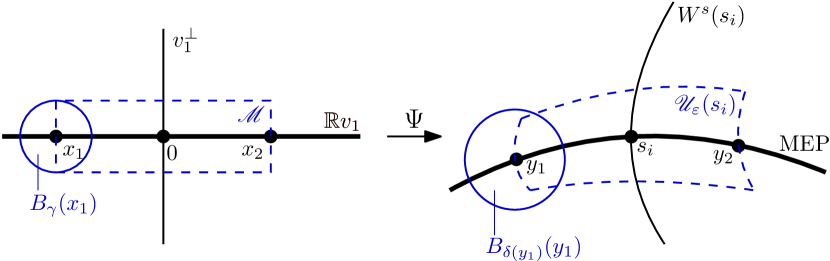
Figure 3: An illustration of the use of the Hartman–Grobman theorem in the proof of Lemma 3.8.

Uniform stability of ${\rm M}$ under gradient descent in a one-sided distance is an immediate corollary of Lemma 3.8:

Lemma 3.10.

For every $\varepsilon>0$, there exists a $\delta>0$ so that

$$d(x,{\rm M})\leq\delta\text{ implies }d(S_{t}(x),{\rm M})\leq\varepsilon\text{ for all }t\geq 0.$$

Proof 3.11.

Let $\mathscr{U}_{\varepsilon}(p)$ be defined as in Lemma 3.8. The open set

$$\mathscr{U}:=\cup_{p\in{\rm M}}\mathscr{U}_{\varepsilon}(p)$$

contains ${\rm M}$, and $x\in\mathscr{U}$ implies $d(S_{t}(x),{\rm M})\leq\varepsilon$ for all $t\geq 0$. Now for any $x\in{\rm M}$, define

$$r(x):=\sup\{\rho>0:B_{\rho}(x)\subset\mathscr{U}\}.$$

The function $r(x)$ is lower semicontinuous, and ${\rm M}$ is compact, so $r(x)$ attains a minimum $\delta$ on ${\rm M}$. We have $\delta>0$ since $\mathscr{U}$ is open. Moreover, $d(x,{\rm M})\leq\delta$ implies $x\in\mathscr{U}$, so $d(S_{t}(x),{\rm M})\leq\varepsilon$ for all $t\geq 0$, as desired.

Lemma 3.8 also implies asymptotic stability of ${\rm M}$ under gradient descent in a one-sided distance:

Lemma 3.12.

There exist an open set $B$ with ${\rm M}\subset B$ and a function ${T:(0,\infty)\rightarrow(0,\infty)}$ so that for any $\varepsilon>0$ and $x\in B$,

$$d(S_{t}(x),{\rm M})\leq\varepsilon\text{ whenever }t\geq T(\varepsilon).$$

Proof 3.13.

For each $p\in{\rm M}$, let $\mathscr{U}_{1}(p)$ be the set constructed in the proof of Lemma 3.8 with $\varepsilon=1$. Define

$$\mathscr{U}:=\cup_{p\in\{m_{1},\dots,m_{k},s_{1},\dots,s_{k-1}\}}\mathscr{U}_{1}(p).$$

We claim that for some time $T$ sufficiently large, the set

(12) $$B^{\prime}:=\cup_{t=0}^{T}S_{-t}(\mathscr{U})$$

contains ${\rm M}$. To see this, we observe that $\cup_{t=0}^{\infty}S_{-t}(\mathscr{U})$ is an open cover of ${\rm M}$. The sets $S_{-t}(\mathscr{U})$ are open, since $\mathscr{U}$ is open and the flow $S_{t}$ is a diffeomorphism. Moreover, these sets cover ${\rm M}$, since they contain the stationary points, and for each ${p\in{\rm M}}$, the trajectory $S_{t}(p)$ converges to a stationary point. Therefore, since ${\rm M}$ is compact it follows that $B^{\prime}$ contains ${\rm M}$ for some finite $T>0$.

Now fix $\varepsilon>0$. Let $B$ be an bounded open subset of $B^{\prime}$ with ${\rm M}\subset B$ and such that $\bar{B}$, the closure of $B$, is contained in $B^{\prime}$. By Lemma 3.10, there exists an open neighborhood $\mathcal{V}_{\varepsilon}$ of ${\rm M}$ so that $x\in\mathcal{V}_{\varepsilon}$ implies $d(S_{t}(x),{\rm M})<\varepsilon$ for all $t\geq 0$. For any $x\in B$, define

$$t(x;\varepsilon):=\inf\{t\geq 0:S_{t}(x)\in\mathcal{V}_{\varepsilon}\}.$$

Observe that $t(x;\varepsilon)$ is finite, since when $x\in B$, $S_{T}(x)\in\mathscr{U}$, and so the trajectory $S_{t}(x)$ converges to one of the stationary points. We claim that $t(x;\varepsilon)$ is upper semicontinuous (as a function of $x$) on $\bar{B}$. By definition of $t(x;\varepsilon)$, for any $\eta>0$, there exists $\eta^{\prime}\in[0,\eta)$ so that $S_{t(x;\varepsilon)+\eta^{\prime}}(x)\in\mathcal{V}_{\varepsilon}$. Moreover, since $\mathcal{V}_{\varepsilon}$ is open and $S_{t(x;\varepsilon)+\eta^{\prime}}$ is continuous, there exists some $\delta>0$ small enough that $S_{t(x;\varepsilon)+\eta^{\prime}}(B_{\delta}(x))\subset V_{\varepsilon}$. Thus, for any $y\in B_{\delta}(x)$,

$$t(y;\varepsilon)\leq t(x;\varepsilon)+\eta^{\prime}\leq t(x;\varepsilon)+\eta,$$

and so $t(x;\varepsilon)$ is upper semicontinuous. Therefore, $t(x;\varepsilon)$ attains a maximum $T(\varepsilon)$ on the compact set $\bar{B}$, hence

$$d(S_{t}(x),{\rm M})<\varepsilon\text{ whenever }t\geq T(\varepsilon),$$

which completes the proof.

Finally, by Lemma 3.6, uniform and asymptotic stability for gradient descent imply the analogous stability properties in Hausdorff distance for the dynamics on curves.

Theorem 3.14.

${\rm M}$ is uniformly stable in the Hausdorff distance under the gradient descent dynamics on curves. Moreover, ${\rm M}$ is asymptotically stable with uniform convergence on $B$ for some compact set $B$ containing an open neighborhood of ${\rm M}$.

Proof 3.15.

We prove only uniform stability; the proof of asymptotic stability is similar. Let $\varepsilon>0$. By Lemma 3.6, there exists $\eta>0$ so that $d(\phi,{\rm M})<\eta$ implies $d_{\rm H}(\phi,{\rm M})<\varepsilon$. Moreover, by Lemma 3.10, there exists $\delta>0$ so that $d(\phi,{\rm M})<\delta$ implies $d(S_{t}(\phi),{\rm M})<\eta$ for all $t\geq 0$. Therefore, if $\phi\in\mathbf{C}(m_{1},m_{k})$ and $d_{\rm H}(\phi,{\rm M})<\delta$, we have $d_{\rm H}(S_{t}(\phi),{\rm M})<\varepsilon$ for all $t\geq 0$. Thus, ${\rm M}$ is uniformly stable in Hausdorff distance under GDDC.

Our stability results guarantee the existence of a Lyapunov function. We begin by constructing an appropriate domain, $B$, for this Lyapunov function. The key property of this domain is forward invariance, i.e. that $x\in B$ implies $S_{t}(x)\in B$ for all $t\geq 0$.

Lemma 3.16.

For some $\delta>0$ there exists a compact, forward invariant set $B$ containing an open neighborhood of ${\rm M}$.

Proof 3.17.

By Lemma 3.10, for any $\varepsilon>0$ there exists a $\delta>0$ so that $d(x,{\rm M})<\delta$ implies $d(S_{t}(x),{\rm M})<\varepsilon$ for all $t\geq 0$. Define

$$\mathscr{N}_{\delta}({\rm M}):=\cup_{p\in{\rm M}}B_{\delta}(p),$$

and

$$B:=\overline{\cup_{\tau\geq 0}S_{\tau}(\mathscr{N}_{\delta}({\rm M}))}.$$

We have $B\supset\mathscr{N}_{\delta}({\rm M})$. Moreover,

$$B\subset\overline{\mathscr{N}_{\varepsilon}({\rm M})},$$

so $B$ is bounded.

To see that $B$ is forward invariant, let $x\in B$. We must show that for any $t\geq 0$, $S_{t}x$ is a limit point of $\cup_{\tau\geq 0}S_{\tau}(\mathscr{N}_{\delta}({\rm M}))$. We first observe that by definition, for any $\varepsilon>0$, there is some $x(\varepsilon)\in\cup_{\tau\geq 0}S_{\tau}(\mathscr{N}_{\delta}({\rm M}))$ with

$$\lvert x-x(\varepsilon)\rvert<\varepsilon.$$

Therefore, for any $\varepsilon>0$,

$$\lvert S_{t}x-S_{t}x(\varepsilon\exp(-tL))\rvert\leq\exp(tL)\lvert x-x(\varepsilon\exp(-tL))\rvert\leq\varepsilon.$$

Thus, since $S_{t}x(\varepsilon\exp(-tL))\in\cup_{\tau\geq 0}S_{\tau}(\mathscr{N}_{\delta}({\rm M}))$, $S_{t}x$ is a limit point, as desired.

We now construct a Lyapunov function for ${\rm M}$ in Hausdorff distance.

Theorem 3.18.

Let $B$ be a compact, forward invariant set containing an open neighborhood of ${\rm M}$. Assume that ${\rm M}$ is asymptotically stable with uniform convergence on $B$. There exists a Lyapunov function $V:\mathbf{C}(m_{1},m_{k},B)\rightarrow[0,\infty)$ for ${\rm M}$.

Proof 3.19.

We adapt the proof of [19, Theorem 1.7.6]. Details appear in Appendix B.

Remark 3.20.

Previous work has analyzed convergence of trajectories of GDDC to ${\rm MEP}$s [2]. It is known that if the limit set of a trajectory is a ${\rm MEP}$, then the trajectory converges to that ${\rm MEP}$ [2, Theorem 3]. This is the case if there are finitely many critical points of the potential $V$ and all are minima or saddles of index one [2, Corollary 4], or if both the potential and the initial curve are piecewise analytic [2, Corollary 7]. However, we are not aware of any results other than our Theorem 3.14 regarding the local asymptotic and uniform stability of individual ${\rm MEP}$s. It is these local stability results which imply that a given MEP can be computed using a discretization of GDDC.

4 Convergence of the String Method

Our main result in this section is Theorem 4.7, which implies that any ${\rm MEP}$ ${\rm M}$ passing alternately through minima and saddles of index one may be approximated to arbitrary accuracy by the string method. The proof uses the existence of a Lyapunov function to show that discretization errors in the string method do not accumulate. Thus, the string method follows the GDDC, converging to a neighborhood of ${\rm M}$ over long times.

For convenience, we analyze only the simplified and improved string method with the linear interpolant. Assume that $I$ is the linear interpolant defined in (4).

We also place consistency and stability assumptions on the numerical integrator:

For some $q\geq 2$ and $D>0$, we have

(13) $$\lvert S_{\Delta t}(x)-\bar{S}_{\Delta t}(x)\rvert\leq D\Delta t^{q}$$

for all $x\in\mathbb{R}^{d}$. In addition,

(14) $$\lvert\bar{S}_{\Delta t}^{n}(x)-\bar{S}_{\Delta t}^{n}(y)\rvert\leq\exp(Ln\Delta t)\lvert x-y\rvert.$$

We note that all commonly used integrators satisfy (13) with $q\geq 2$, and many integrators satisfy (14); see [19]. In particular, for Euler’s method,

$$\lvert\bar{S}_{\Delta t}(x)-\bar{S}_{\Delta t}(y)\rvert =x-y-\Delta t(-\nabla V(x)-\nabla V(y))\leq(1+\Delta tL)\lvert x-y\rvert.$$

Therefore, since $1+\Delta tL\leq\exp(\Delta tL)$,

$$\lvert\bar{S}_{\Delta t}^{n}(x)-\bar{S}_{\Delta t}^{n}(y)\rvert\leq(1+\Delta tL)^{n}\lvert x-y\rvert\leq\exp(Ln\Delta t)\lvert x-y\rvert.$$

We now estimate the error introduced when reparametrizing the string.

Lemma 4.1.

Let $x\in\mathbf{S}^{N+1}$. We have

$$d_{\rm H}(Ix,IRx)\leq\frac{m(x)}{2}.$$

Proof 4.2.

First, we observe that for any $x\in\mathbf{S}^{N+1}$, we have $m(Rx)\leq m(x)$. To see this, let $s(Ix,a,b)$ denote the arc-length along $Ix$ between $a$ and $b$. We have

$$|Rx_{i}-Rx_{i+1}|\leq s(Ix,Rx_{i},Rx_{i+1})=\frac{\ell(x)}{N}=\frac{\sum_{i=0}^{k-1}\lvert x_{i+1}-x_{i}\rvert}{N}\leq m(x).$$

Now let $y\in IRx$, and suppose that $y$ is between $Rx_{i}$ and $Rx_{i+1}$. We have

$$\min\{|Rx_{i}-y|,|Rx_{i+1}-y|\}\leq\frac{1}{2}|Rx_{i}-Rx_{i+1}|\leq\frac{m(Rx)}{2}\leq\frac{m(x)}{2}.$$

Therefore, since $Rx_{i}\in Ix$ and $Rx_{i+1}\in Ix$, $d(IRx,Ix)\leq\frac{m(x)}{2}$. Now let $y\in Ix$, and suppose that $y=I(\ell^{\ast}(x),x)(\alpha)$ for some $\alpha\in\left[\frac{i}{N},\frac{i+1}{N}\right]$. We have

$$\min\{|Rx_{i}-y|,|Rx_{i+1}-y|\}\leq\frac{1}{2}s(Ix,Rx_{i},Rx_{i+1})\leq\frac{m(x)}{2},$$

so $d(Ix,IRx)\leq\frac{Kh}{2}$. We conclude that $d_{\rm H}(Ix,IRx)\leq\frac{m(x)}{2}$.

We now show that reparametrization occurs only after each image has been advanced at least by a certain time $\tau>0$. This is crucial for the numerical analysis, since the upper bound on reparametrization error in Lemma 4.1 does not have a factor involving the time step $\Delta t$. This upper bound suffices because we do not consider whether the string method approximates GDDC in the limit as $\Delta t\rightarrow 0$. Instead, we are interested only in the convergence of strings to ${\rm M}$ over long times.

Lemma 4.3.

Let $x\in\mathbf{S}^{N+1}$. Define

$$\tau:=\frac{\log(K)}{L}$$

We have

$$m(\bar{S}^{n}_{\Delta t}(x))\leq Km(x)\text{ for all }0\leq n\leq\left\lfloor\frac{\tau}{\Delta t}\right\rfloor.$$

Proof 4.4.

By (14), we have

$$\lvert\bar{S}^{n}_{\Delta t}(x_{i+1})-\bar{S}^{n}_{\Delta t}(x_{i})\rvert\leq\exp(Ln\Delta t)\lvert x_{i+1}-x_{i}\rvert\leq\exp(L\tau)m(x)\leq Km(x)$$

for all $i=1,\dots,k$.

Finally, we estimate the error resulting from evolving only the images $x_{i}$ by gradient descent in each step, not the entire interpolated curve $Ix$.

Lemma 4.5.

Let $x\in\mathbf{S}^{N+1}$ and let $\tau$ be defined as in Lemma 4.3. There exists a constant $C>0$ depending only on $V$ and $\tau$ so that

$$d_{\rm H}(S_{\Delta t}Ix,IS_{\Delta t}x)\leq Cm(x)^{2}\Delta t\text{ for all }0\leq\Delta t\leq\tau.$$

Proof 4.6.

Let $x\in\mathbf{S}^{N+1}$. Fix $\alpha\in[0,1]$ and $i\in\{0,\dots,N\}$. Let

$$\bar{x}=(1-\alpha)x_{i}+\alpha x_{i+1}.$$

Write

$$y=x_{i+1}-x_{i}.$$

For any $z\in\mathbb{R}^{d}$, define $\partial_{z}$ to be the derivative in direction $z$, so for example

$$\partial_{z}S_{t}(x)=\left.\frac{d}{d\varepsilon}\right\rvert_{\varepsilon=0}S_{t}(x+\varepsilon z).$$

Since $\nabla V$ is twice continuously differentiable, the flow $S_{t}(x)$ is also twice continuously differentiable as a function of $(t,x)$ by [3, Theorem 1.3]. Therefore, by Taylor’s theorem, for some $x^{\prime}$ and $x^{\prime\prime}$ in the convex hull of $\{x_{i},x_{i+1}\}$, we have

$$S_{\Delta t}(x_{i})-S_{\Delta t}(\bar{x})=-\alpha\partial_{y}S_{\Delta t}(\bar{x})+\frac{1}{2}\alpha^{2}\partial_{y}^{2}S_{\Delta t}(x^{\prime}),$$

and

$$S_{\Delta t}(x_{i+1})-S_{\Delta t}(\bar{x})=(1-\alpha)\partial_{y}S_{\Delta t}(\bar{x})+\frac{1}{2}(1-\alpha)^{2}\partial_{y}^{2}S_{\Delta t}(x^{\prime\prime}).$$

It follows that

$$\lvert(1-\alpha)S_{\Delta t}x_{i}+\alpha S_{\Delta t}x_{i+1}-S_{\Delta t}(\bar{x})\rvert \leq\frac{1}{2}\sup_{z\in\mathbb{R}^{d}}\left\lvert\partial_{y/\lvert y\rvert}^{2}S_{\Delta t}(z)\right\rvert\lvert y\rvert^{2}$$

(15) $$\leq\frac{1}{2}\sup_{z\in\mathbb{R}^{d}}\left\lvert\partial_{w}^{2}S_{\Delta t}(z)\right\rvert m(x)^{2},$$

where we define $w=y/\lvert y\rvert$.

$S_{t}(x)$ solves the gradient descent initial value problem

$$\begin{dcases}\frac{d}{dt}S_{t}(x)&=-\nabla V(S_{t}(x))\\ S_{0}(x)&=x.\end{dcases}$$

Differentiating this initial value problem twice with respect to $x$ yields

(16) $$\begin{dcases}\frac{d}{dt}\partial_{w}^{2}S_{t}(x)&=\Gamma(t)+A(t)\partial_{w}^{2}S_{t}(x)\\ \partial_{w}^{2}S_{0}(x)&=0.\end{dcases}$$

where

$$\Gamma(t)_{q} :=-\sum_{\ell,m=1}^{d}\frac{\partial^{3}V}{\partial x_{q}\partial x_{\ell}\partial x_{m}}(S_{t}(x))\partial_{w}S_{t}(x)_{\ell}\partial_{w}S_{t}(x)_{m} \text{ for }q=1,\dots,d\text{ and }$$

$$A(t)_{q\ell} :=-\frac{\partial^{2}V}{\partial x_{q}\partial x_{\ell}}(S_{t}(x)) \text{ for }q,\ell=1,\dots,d.$$

(Here, $\partial_{w}S_{t}(x)_{\ell}$ and $\partial_{w}^{2}S_{t}(x)_{\ell}$ denote the $\ell$’th coordinate components of $\partial_{w}S_{t}(x)_{\ell}$ and $\partial_{w}^{2}S_{t}(x)_{\ell}$, respectively.)

Since $\partial_{w}^{2}S_{0}(x)=0$, we have $\lvert\partial_{w}^{2}S_{t}(x)\rvert\leq C(x)t$ for any fixed $x\in\mathbb{R}^{d}$. However, it is not immediately clear that this estimate holds with a constant independent of $x$. To prove this, observe that since $\nabla V$ is Lipschitz with constant $L$, we have

$$\sup_{t\in[0,\infty)}\lVert A(t)\rVert_{2}\leq\sup_{z\in\mathbb{R}^{d}}\left\lVert\frac{\partial^{2}V}{\partial x_{q}\partial x_{\ell}}(z)\right\rVert_{2}\leq L,$$

where $\lVert\cdot\rVert_{2}$ is the operator norm induced by Euclidean distance $\lvert\cdot\rvert$. Moreover, $S_{t}$ is Lipschitz with constant $\exp(Lt)$, so

$$\partial_{w}S_{t}(x)\leq\exp(Lt)\lvert w\rvert=\exp(Lt).$$

By Assumption 3,

$$\left\lvert\frac{\partial^{3}V}{\partial x_{q}\partial x_{\ell}\partial x_{m}}(S_{t}(x))\right\rvert\leq C_{3}.$$

Thus,

$$\Gamma(t)\leq dC_{3}\exp(2Lt).$$

It then follows from (16) that

$$\lVert\partial_{w}^{2}S_{t}(x)\rVert \leq\int_{0}^{t}\lVert\Gamma(s)\rVert\,ds+\int_{0}^{t}\lVert A(s)\rVert_{2}\lVert\partial_{w}^{2}S_{s}(x)\rVert\,ds$$

$$\leq\frac{dC_{3}}{2L}(\exp(2Lt)-1)+L\int_{0}^{t}\lVert\partial_{w}^{2}S_{s}(x)\rVert\,ds.$$

Therefore, by Grönwall’s inequality,

(17) $$\lVert\partial_{w}^{2}S_{t}(x)\rVert\leq\frac{dC_{3}}{2L}(\exp(2Lt)-1)\exp(Lt).$$

Finally, by (15) and (17), we have

$$\lvert(1-\alpha)S_{\Delta t}x_{i}+\alpha S_{\Delta t}x_{i+1}-S_{\Delta t}(\bar{x})\rvert \leq\frac{dC_{3}}{2L}(\exp(2L\Delta t)-1)\exp(L\tau)m(x)^{2}$$

$$\leq dC_{2}\exp(3L\tau)m(x)^{2}\Delta t$$

$$\leq dC_{2}K^{3}m(x)^{2}\Delta t$$

for all $\Delta t\leq\tau$. This proves the result, since every point $y\in IS_{\Delta t}x$ takes the form

$$y=(1-\alpha)S_{\Delta t}x_{i}+\alpha S_{\Delta t}x_{i+1}$$

for some $i\in\{0,\dots,N\}$ and $\alpha\in[0,1]$, and every point $z\in S_{\Delta t}Ix$ takes the form

$$z=S_{\Delta t}((1-\beta)x_{j}+\beta x_{j+1}).$$

for some $j\in\{0,\dots,N\}$ and $\beta\in[0,1]$.

We now prove our convergence result for the simplified and improved string method. We note that some aspects of the proof were inspired by a result concerning the persistence of attractors of ODEs under discretization; see [12] and [19, Theorem 7.5.1].

Theorem 4.7.

There exist $h_{0}>0$, $r_{0}>0$, $N_{0}>0$, and a function $e:(0,h_{0})\times(0,\tau)\rightarrow(0,\infty)$ with

$$\lim_{h,\Delta t\rightarrow 0^{+}}e(h,\Delta t)=0$$

such that if $d_{\rm H}(Ix^{0},{\rm M})<r_{0}$ and $h<h_{0}$, then

$$d_{\rm H}(Ix^{n},{\rm M})\leq e(h,\Delta t)\text{ for all }n>N_{0}.$$

Proof 4.8.

First, one must show that there exist $h_{0}>0$, $r_{0}>0$, and $t_{\rm{max}}>0$ so that if $h<h_{0}$, $\Delta t\leq t_{\rm{max}}$, and $d_{\rm H}(Ix^{0},{\rm M})\leq r_{0}$, then $Ix^{\ell}$ belongs to the domain $\mathscr{W}$ of $W$ for all $\ell\geq 0$. We prove this in Appendix C.

Once it is established that the entire trajectory of the string method lies in the domain of $W$, the result follows from a variation of parameters formula involving $W$. By the contraction property (6) and Lipschitz property (7) of the Lyapunov function, we have

$$W(Ix^{\ell+1}) \leq W(S_{\Delta t}Ix^{\ell})+\lvert W(Ix^{\ell+1})-W(S_{\Delta t}Ix^{\ell})\rvert$$

$$\leq\exp(-c\Delta t)W(Ix^{\ell})+d_{\rm H}(Ix^{\ell+1},S_{\Delta t}Ix^{\ell})$$

(18) $$\leq\exp(-c\Delta t)W(Ix^{\ell})+d_{\rm H}(Ix^{\ell+1},I\bar{S}_{\Delta t}x^{\ell})$$

$$\qquad\qquad+d_{\rm H}(I\bar{S}_{\Delta t}x^{\ell},IS_{\Delta t}x^{\ell})+d_{\rm H}(IS_{\Delta t}x^{\ell},S_{\Delta t}Ix^{\ell})$$

(19) $$\leq\exp(-c\Delta t)W(Ix^{\ell})+R_{\ell}+T_{\ell}+C_{\ell},$$

where we define

$$R_{\ell} :=d_{\rm H}(Ix^{\ell+1},IS_{\Delta t}x^{\ell}),$$

$$T_{\ell} :=d_{\rm H}(I\bar{S}_{\Delta t}x^{\ell},IS_{\Delta t}x^{\ell}),\text{ and }$$

$$C_{\ell} :=d_{\rm H}(IS_{\Delta t}x^{\ell},S_{\Delta t}Ix^{\ell}).$$

The term $R_{\ell}$ is associated with reparametrization, $T_{\ell}$ is the truncation error of the numerical integrator, and $C_{\ell}$ is associated with commuting evolution by $S_{\Delta t}$ and interpolation.

By induction using (19), we have the variation of parameters formula

(20) $$W(Ix^{\ell}) \leq\exp(-c\ell\Delta t)W(Ix^{0})+\sum_{j=0}^{\ell-1}\exp(-c(\ell-j-1)\Delta t)(R_{j}+T_{j}+C_{j}).$$

Assumption 4 implies

$$T_{\ell}\leq D\Delta t^{q},$$

since when $I$ is the linear interpolant

$$d_{\rm H}(Ix,Iy)\leq\max_{i=0,\dots,N+1}\lvert x_{i}-y_{i}\rvert$$

for any $x,y\in\mathbf{S}^{N+1}$. Moreover, by Lemma 4.5,

$$C_{\ell}\leq C(Kh)^{2}\Delta t.$$

Therefore,

$$\sum_{j=0}^{\ell-1}\exp(-c(\ell-j-1)\Delta t)(T_{j}+C_{j}) \leq\frac{(D\Delta t^{q}+C(Kh)^{2})\Delta t(1-\exp(-c\ell\Delta t))}{1-\exp(-c\Delta t)}$$

$$\leq\frac{(D\Delta t^{q-1}+C(Kh)^{2})(1-\exp(-c\ell\Delta t))}{c}$$

(21) $$\leq\frac{D\Delta t^{q-1}+C(Kh)^{2}}{c}.$$

(The second inequality above follows since $x\mapsto 1-\exp(-cx)$ is a concave fucntion with the tangent line $x\mapsto cx$ at $x=0$, so $1-\exp(-c\Delta t)\leq c\Delta t$.)

The term $R_{\ell}$ is zero unless reparametrization occurs in the $\ell+1$’st step of the string method. Let $r_{i}$ be the step in which the $i$’th reparametrization occurs. By Lemma 4.3,

$$r_{i}\geq\left\lceil\frac{\tau}{\Delta t}\right\rceil i.$$

When reparametrization does occur in the $\ell+1$’st step, we have $m(x^{\ell})\leq Kh$, but $m(x^{\ell+1})>Kh$. However, since $S_{\Delta t}$ is Lipschitz with constant $\exp(L\Delta t)$,

$$m(x^{\ell+1})\leq\exp(L\Delta t)Kh.$$

Therefore, by Lemma 4.1

$$R_{\ell}\leq\frac{\exp(L\Delta t)Kh}{2}.$$

Thus, we have

$$\sum_{j=0}^{\ell-1}\exp(-c(\ell-j-1)\Delta t)R_{j} \leq\sum_{j=0}^{\infty}\exp(-c(\ell-j-1)\Delta t)R_{j}$$

$$\leq\frac{\exp(L\Delta t)Kh}{2}\sum_{i=1}^{\infty}\exp\left(-ci\Delta tr_{i}\right)$$

$$\leq\frac{\exp(L\Delta t)Kh}{2}\sum_{i=1}^{\infty}\exp\left(-ci\left\lceil\frac{\tau}{\Delta t}\right\rceil\Delta t\right)$$

(22) $$\leq\frac{\exp(L\Delta t)Kh}{2}\frac{1}{1-\exp(-c\tau)}.$$

We conclude that

$$W(Ix^{\ell}) \leq\exp(-c\ell\Delta t)W(Ix^{0})+\frac{\exp(L\Delta t)Kh}{2(1-\exp(-c\tau))}+\frac{D\Delta t^{q-1}+C(Kh)^{2}}{c}$$

$$\leq\exp(-c\ell\Delta t)r_{0}+\frac{\exp(L\Delta t)Kh}{2(1-\exp(-c\tau))}+\frac{D\Delta t^{q-1}+C(Kh)^{2}}{c}.$$

(The second inequality above follows from the Lipschitz property of $W$ (7) and ${W({\rm M})=0}$ using that $d_{\rm H}(Ix^{0},{\rm M})\leq r_{0}$.) Therefore, for some $N_{0}>0$ depending only on $r_{0}$, $\ell\geq N_{0}$ implies

$$W(Ix^{\ell})\leq\frac{\exp(L\Delta t)Kh}{(1-\exp(-c\tau))}+\frac{2(D\Delta t^{q-1}+C(Kh)^{2})}{c}.$$

Thus, for $\ell\geq N_{0}$,

$$d_{\rm H}(Ix^{\ell},{\rm M})\leq\alpha^{-1}\left(\frac{\exp(L\Delta t)Kh}{(1-\exp(-c\tau))}+\frac{2(D\Delta t^{q-1}+C(Kh)^{2})}{c}\right)=:e(h,\Delta t)$$

by (8) and the monotonicity of $\alpha$. We observe that since $\alpha(0)=0$ and $\alpha$ is strictly increasing

$$\lim_{h,\Delta t\rightarrow 0^{+}}e(h,\Delta t)=0,$$

which concludes the proof.

Appendix A Proof of Lemma 3.6

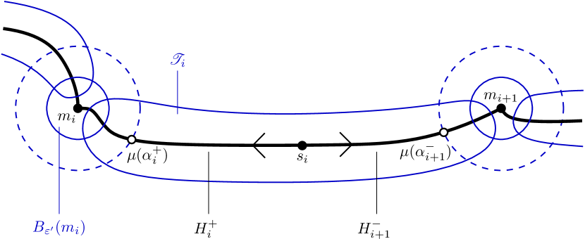
Figure 4: A depiction of the neighborhoods constructed in the proof of Lemma 3.6. The bold black line represents ${\rm M}$. The arrows point in the direction of gradient descent along the heteroclinics $H_{i}^{+}$ and $H_{i}^{-}$ connecting $s_{i}$ to $m_{i}$ and $m_{i+1}$. The blue dashed balls are $B_{2\varepsilon^{\prime}}(m_{i})$ and $B_{2\varepsilon^{\prime}}(m_{i+1})$.

Proof A.1.

We adapt the argument based on tubular neighborhoods outlined after the statement of Lemma 3.6. To allow for kinks at the minima, we devise an analogue of a tubular neighborhood consisting of tubes where ${\rm M}$ is smooth connected by balls surrounding the minima as in Figure 4.

Let $\varepsilon>0$. Since each minimum $m_{i}$ is linearly stable, there exists $\varepsilon_{i}>0$ so that $x\in B_{\varepsilon_{i}}(m_{i})$ implies $\lvert S_{t}x-m_{i}\rvert$ is strictly decreasing with $t$. Let

$$\varepsilon^{\prime}=\min\left\{\frac{\varepsilon}{6},\frac{\min_{i=1,\dots,k}\varepsilon_{i}}{2}\right\}.$$

Observe that the balls $B_{2\varepsilon^{\prime}}(m_{i})$ are disjoint, since the basins of attraction of the minima $m_{i}$ under the gradient flow are disjoint.

Let $H_{i}^{+}$ be the heteroclinic connecting $m_{i}$ with $s_{i}$, and $H_{i+1}^{-}$ the heteroclinic connecting $s_{i}$ with $m_{i+1}$, as in Figure 1. We claim that for any $i=1,\dots,k-1$, the curve segment

$$M_{i}=H_{i}^{+}\cup H_{i+1}^{-}\setminus B_{\frac{\varepsilon^{\prime}}{2}}(m_{i})\cup B_{\frac{\varepsilon^{\prime}}{2}}(m_{i+1})$$

is a ${\rm C}^{2}$-embedded submanifold of $\mathbb{R}^{d}$. To prove this, observe that in an open neighborhood of the the saddle point $s_{i}$, $M_{i}$ coincides with the local unstable manifold of $s_{i}$. Since $V\in{\rm C}^{3}$, by the invariant manifold theorem[18, Theorem 5.2], the local unstable manifold is a ${\rm C}^{2}$-embedded submanifold of $\mathbb{R}^{d}$. Now since $M_{i}$ lies on the pair of heteroclinics $H_{i}^{+}$ and $H_{i+1}^{-}$, for some time $T>0$, the whole of $M_{i}$ is contained in the image under $S_{T}$ of the part coinciding with the local unstable manifold. The flow map $S_{T}$ is a diffeomorphism, and since $V\in{\rm C}^{3}$ we have $S_{T}\in{\rm C}^{2}$ by [3, Theorem 1.3]. Thus, $M_{i}$ is a ${\rm C}^{2}$-embedded submanifold.

It follows by [13, Theorem 10.19] that $M_{i}$ has a tubular neighborhood. (The statement of [13, Theorem 10.19] assumes a ${\rm C}^{\infty}$-embedded submanifold. However, the proof requires only a ${\rm C}^{2}$-embedded submanifold.) In particular, for any radius $\rho_{i}>0$ small enough, there exist an open neighborhood $\mathscr{T}_{i}$ with ${M_{i}\subset\mathscr{T}_{i}}$ and a continuous retraction $r_{i}:\mathscr{T}_{i}\rightarrow M_{i}$ such that

$$\lvert x-r_{i}(x)\rvert<\rho_{i}.$$

For all $i=1,\dots,k-1$, let $0<\rho_{i}<\varepsilon^{\prime}$ be small enough that a tubular neighborhood exists. Since the closures of the curve segments $M_{i}$ are disjoint, we may assume that the tubular neighborhoods $\mathscr{T}_{i}$ are disjoint, reducing $\rho_{i}$ if necessary. Moreover, we may assume that $\mathscr{T}_{i}\cap B_{2\varepsilon^{\prime}}(m_{k})\neq\emptyset$ only for $k=i,i+1$.

Since ${\rm M}$ does not intersect itself, it is homeomorphic to an interval. That is, there exists a continuous bijection $\mu:[0,1]\rightarrow{\rm M}$ with continuous inverse $\mu^{-1}:{\rm M}\rightarrow[0,1]$. (Here, we equip ${\rm M}$ with the subspace topology inherited from $\mathbb{R}^{d}$.) We may assume that for some $0=\alpha_{1}<\alpha_{2}<\dots<\alpha_{k}=1$,

$$\mu(\alpha_{i})=m_{i}.$$

For each $i=1,\dots,k-1$, define

$$\alpha_{i}^{+}:=\sup\{\alpha\in[0,1]:\mu(\alpha)\in B_{2\varepsilon^{\prime}}(m_{i})\},$$

and let $\alpha_{k}^{+}=1$. Similarly, for $i=2,\dots,k$, define

$$\alpha_{i+1}^{-}:=\inf\{\alpha\in[0,1]:\mu(\alpha)\in B_{2\varepsilon^{\prime}}(m_{i+1})\},$$

and let $\alpha_{1}^{-}=0$. We claim that

(23) $$\mu(\alpha)\in B_{2\varepsilon^{\prime}}(m_{i})\text{ iff }\alpha\in[\alpha_{i}^{-},\alpha_{i}^{+}].$$

To prove (23), observe that by continuity of $\mu$, $\mu(\alpha_{i}^{+})\in\partial B_{2\varepsilon^{\prime}}(m_{i})$. In fact, since $\lvert S_{t}(x)-m_{i}\rvert$ is strictly decreasing on $B_{2\varepsilon^{\prime}}(m_{i})$, the heteroclinic trajectory $H_{i}^{+}$ intersects $\partial B_{2\varepsilon^{\prime}}(m_{i})$ only at $\mu(\alpha^{+}_{i})$. If we had $\lvert\mu(\alpha)-m_{i}\rvert>2\varepsilon^{\prime}$ for some $\alpha\in[\alpha_{i},\alpha_{i}^{+}]$, the intermediate value theorem would imply the existence of a second distinct point of intersection between $H_{i}^{+}$ and $\partial B_{2\varepsilon^{\prime}}(m_{i})$, since $\mu$ is a bijection. Therefore, $\mu([\alpha_{i},\alpha_{i}^{+}])\subset B_{2\varepsilon^{\prime}}(m_{i})$. A similar argument involving the heteroclinic $H_{i}^{-}$ shows $\mu([\alpha_{i}^{-},\alpha_{i}])\subset B_{2\varepsilon^{\prime}}(m_{i})$, and (23) follows.

We will now construct an analogue $\Pi$ of the retraction $r_{i}$ for the entire ${\rm MEP}$ ${\rm M}$. For convenience, instead of mapping onto ${\rm M}$, $\Pi$ will take values in $[0,1]$, the domain of the parametrization $\mu$ of ${\rm M}$. We handle kinks at minima by letting $\Pi$ take a constant value on a ball surrounding each minimum. We begin by defining for each $i=1,\dots,k-1$ the three continuous functions

$$p_{i}^{+}:B_{\varepsilon^{\prime}}(m_{i})\rightarrow\mathbb{R} \qquad\text{ by }p_{i}^{+}(x)=\alpha_{i}^{+},$$

$$p_{i}:\mathscr{T}_{i}\rightarrow\mathbb{R} \qquad\text{ by }p_{i}(x)=\min\{\alpha_{i+1}^{-},\max\{\alpha_{i}^{+},\mu^{-1}\circ r_{i}(x)\}\},\text{ and }$$

$$p_{i+1}^{-}:B_{\varepsilon^{\prime}}(m_{i+1})\rightarrow\mathbb{R} \qquad\text{ by }p_{i+1}^{-}(x)=\alpha_{i+1}^{-}.$$

These functions will be the constituent parts of our retraction $\Pi$. We claim that $p_{i}^{-}$, $p_{i}$, and $p_{i}^{+}$ agree where their domains intersect. To verify this, it will suffice to show that

$$\mu^{-1}\circ r_{i}(x) \leq\alpha_{i}^{+} \text{ for }x\in B_{\varepsilon^{\prime}}(m_{i})\cap\mathscr{T}_{i},\text{ and }$$

$$\mu^{-1}\circ r_{i}(x) \geq\alpha_{i+1}^{-} \text{ for }x\in B_{\varepsilon^{\prime}}(m_{i+1})\cap\mathscr{T}_{i}.$$

Let $x\in B_{\varepsilon^{\prime}}(m_{i})\cap\mathscr{T}_{i}$. Then

$$\lVert r_{i}(x)-m_{i}\rVert\leq\lVert r_{i}(x)-x\rVert+\lVert x-m_{i}\rVert\leq\rho_{i}+\varepsilon^{\prime}\leq 2\varepsilon^{\prime},$$

and so $r_{i}(x)\in B_{2\varepsilon^{\prime}}(m_{i})$. Therefore, $\mu^{-1}\circ r_{i}(x)\leq\alpha^{+}_{i}$ by (23). Similarly, $x\in B_{\varepsilon^{\prime}}(m_{i+1})\cap\mathscr{T}_{i}$ implies $\mu^{-1}\circ r_{i}(x)\geq\alpha_{i+1}^{-}$. Thus, the three functions agree on the intersections of their domains. Therefore, since the domains are open, they define a single continuous function $\pi_{i}$ on

$$\mathscr{U}_{i}:=B_{\varepsilon^{\prime}}(m_{i})\cup\mathscr{T}_{i}\cup B_{\varepsilon^{\prime}}(m_{i+1}).$$

We now patch together the functions $\pi_{i}$ to construct our retraction $\Pi$. First, define $\tilde{\pi}_{i}:\mathscr{U}_{i}\rightarrow[0,1]$ by

$$\tilde{\pi}_{i}(x)=\pi_{i}(x)-\sum_{j=2}^{i}\alpha_{j}^{+}-\alpha_{j}^{-}.$$

The functions $\tilde{\pi}_{i}$ are continuous, have open domains, and agree on the intersections of their domains. In fact, for $i=1,\dots,k-1$, the functions $\tilde{\pi}_{i}$ and $\tilde{\pi}_{i+1}$ both take the value

$$\alpha_{i+1}^{-}-\sum_{j=2}^{i+1}\alpha_{j}^{+}-\alpha_{j}^{-}.$$

on $B_{\varepsilon^{\prime}}(m_{i+1})=\mathscr{U}_{i}\cap\mathscr{U}_{i+1}$. The domains $\mathscr{U}_{i}$ and $\mathscr{U}_{j}$ do not intersect if $\lvert i-j\rvert\geq 2$. Therefore, the functions $\tilde{\pi}_{i}$ define a single continuous function $\Pi$ on

$$\mathscr{U}:=\cup_{i=1}^{K-1}\mathscr{U}_{i}.$$

Since $\mathscr{U}$ is open and ${\rm M}$ is compact, there exists some $\eta>0$ so that $d(x,{\rm M})\leq\eta$ implies $x\in\mathscr{U}$. We claim that the conclusion of the lemma holds for this $\eta$. To see this, let $\phi\in\mathbf{C}(m_{1},m_{k})$ with $d(\phi,{\rm M})\leq\eta$. We have

$$\Pi(m_{1})=\alpha_{1}^{+}\text{ and }\Pi(m_{k})=\alpha_{k}^{-}-\sum_{j=1}^{k-1}\alpha_{j}^{+}-\alpha_{j}^{-}.$$

Therefore, by the intermediate value theorem,

(24) $$\Pi(\phi)\supset\left[\alpha_{1}^{+},\alpha_{k}^{-}-\sum_{j=1}^{k-1}\alpha_{j}^{+}-\alpha_{j}^{-}\right].$$

Now let $x\in{\rm M}$. By (24), there exists some $y\in\phi$ so that $\Pi(y)=\Pi(x)$. To complete the proof, we will show that $\lvert x-y\rvert\leq\varepsilon$. We distinguish two cases: Either $\Pi(x)\neq\Pi(m_{i})$ for any $i\in\{1,\dots,k\}$ or else $\Pi(x)=\Pi(m_{i})$ for some $i\in\{1,\dots,k\}$. In the first case, $y$ lies in a tube $\mathscr{T}_{i}$ for some $i$, and $x=r_{i}(y)$. Therefore,

$$\lvert x-y\rvert<\rho_{i}<\varepsilon^{\prime}<\varepsilon.$$

In the second case, we have $\Pi(y)=\Pi(x)=\Pi(m_{i})$. We claim that for any $z\in\mathscr{U}$,

(25) $$\Pi(z)=\Pi(m_{i})\text{ implies }z\in B_{3\varepsilon^{\prime}}(m_{i}).$$

If so, then

$$\lvert x-y\rvert\leq\lvert x-m_{i}\rvert+\lvert y-m_{i}\rvert\leq 3\varepsilon^{\prime}+3\varepsilon^{\prime}\leq\varepsilon.$$

To prove (25), we observe that if $\Pi(z)=\Pi(m_{i})$, then $z\in\mathscr{U}_{i}\cup\mathscr{U}_{i-1}$. Suppose that $z\in\mathscr{U}_{i}$. On the one hand, if $z\in B_{\varepsilon^{\prime}}(m_{i})$, then (25) holds trivially. On the other hand, if $z\notin B_{\varepsilon^{\prime}}(m_{i})$, then $z\in\mathscr{T}_{i}$. In that case, since $\Pi(z)=\Pi(m_{i})$,

$$\mu^{-1}\circ r_{i}(z)\in[\alpha_{i},\alpha_{i}^{+}],$$

so by (23), $r_{i}(z)\in B_{2\varepsilon^{\prime}}(m_{i})$. Therefore,

$$\lvert z-m_{i}\rvert\leq\lvert z-r_{i}(z)\rvert+\lvert r_{i}(z)-m_{i}\rvert\leq\varepsilon^{\prime}+2\varepsilon^{\prime}=3\varepsilon^{\prime}.$$

This concludes the proof of (25), hence the proof of Lemma 3.6.

Appendix B Proof of Theorem 3.18

Proof B.1.

Let $B\subset\mathbb{R}^{d}$ be a compact, forward invariant set containing ${\rm M}$. We will construct a Lyapunov function for ${\rm M}$, defined on the set $\mathbf{C}(m_{1},m_{2},B)$.

Define $G_{k}:[0,\infty)\rightarrow[0,\infty)$ by

$$G_{k}(x):=\max\{0,x-1/k\}.$$

Let $c>0$. For any $\phi\in\mathbf{C}(m_{1},m_{2},B)$, define

$$V_{k}(\phi):=\sup_{\tau\geq 0}\exp(c\tau)G_{k}(d_{\rm H}(S_{\tau}(\phi),{\rm M})).$$

We note that $V_{k}$ is finite, since asymptotic stability on $B$ implies $G_{k}(S_{\tau}(\phi))=0$ for sufficiently large $\tau$. We will use the functions $V_{k}$ for $k=1,\dots,\infty$ to construct a Lyapunov function.

First, we observe that $V_{k}$ has the contraction property (6) of a Lyapunov function, since

$$V_{k}(S_{t}(\phi)) =\sup_{\tau\geq 0}\exp(c\tau)G_{k}(d_{\rm H}(S_{t+\tau}(\phi),{\rm M}))$$

$$=\exp(-ct)\sup_{\tau\geq 0}\exp(c(t+\tau))G_{k}(d_{\rm H}(S_{t+\tau}(\phi),{\rm M}))$$

$$=\exp(-ct)\sup_{\tau\geq t}\exp(c\tau)G_{k}(d_{\rm H}(S_{\tau}(\phi),{\rm M}))$$

(26) $$\leq\exp(-ct)V_{k}(\phi).$$

We now find a Lipschitz constant for $V_{k}$. ${\rm M}$ is asymptotically stable with uniform convergence on $B$, and so for each $k\in\mathbb{N}$ there exists $T(1/k)$ so that for any $\phi\in\mathbf{C}(m_{1},m_{2},B)$,

$$d_{\rm H}(S_{t}\phi,{\rm M})\leq 1/k\text{ whenever }T(1/k)\leq t.$$

Therefore, for any $\phi,\psi\in\mathbf{C}(m_{1},m_{2},B)$, we have

$$\lvert V_{k}(\phi)-V_{k}(\psi)\rvert \leq\sup_{\tau=0}\exp(c\tau)\lvert G_{k}(d_{\rm H}(S_{\tau}\phi,{\rm M}))-G_{k}(d_{\rm H}(S_{\tau}\psi,{\rm M}))\rvert$$

$$=\sup_{0\leq\tau\leq T(1/k)}\exp(c\tau)\lvert G_{k}(d_{\rm H}(S_{\tau}\phi,{\rm M}))-G_{k}(d_{\rm H}(S_{\tau}\psi,{\rm M}))\rvert$$

$$\leq\sup_{0\leq\tau\leq T(1/k)}\exp(c\tau)\lvert d_{\rm H}(S_{\tau}\phi,{\rm M})-d_{\rm H}(S_{\tau}\psi,{\rm M})\rvert$$

$$\leq\sup_{0\leq\tau\leq T(1/k)}\exp(c\tau)d_{\rm H}(S_{\tau}\phi,S_{\tau}\psi)$$

$$\leq\sup_{0\leq\tau\leq T(1/k)}\exp(c\tau)\exp(L\tau)d_{\rm H}(\phi,\psi)$$

$$\leq\exp((L+c)T(1/k))d_{\rm H}(\phi,\psi),$$

It follows that

(27) $$L_{k}:=\exp((L+c)T(1/k))$$

is a Lipschitz constant for $V_{k}$.

We claim that $V:\mathbf{C}(m_{1},m_{2},B)\rightarrow[0,\infty)$ defined by

$$V(\phi):=\sum_{k=1}^{\infty}\frac{L_{k}^{-1}V_{k}(\phi)}{2^{k}}$$

is a Lyapunov function for ${\rm M}$ on $B$. To see that the sum defining $V$ converges, we observe that

$$0\leq V_{k}(\phi)\leq V_{k}({\rm M})+L_{k}d_{\rm H}(\phi,{\rm M})\leq L_{k}d_{\rm H}(\phi,{\rm M}),$$

which implies

(28) $$V(\phi)\leq d_{\rm H}(\phi,{\rm M}).$$

The contraction property (6) and Lipschitz bound (7) in the definition of Lyapunov function follow from (26) and (27), respectively. The upper bound in property (8) follows from (28).

Thus, it remains only to show the lower bound in (8); that is, we must show

$$\alpha(d_{\rm H}(\phi,{\rm M}))\leq V(\phi)$$

for some continuous strictly increasing function $\alpha$ with $\alpha(0)=0$. To see this observe that if $d_{\rm H}(\phi,{\rm M})\geq 1$, then

$$V(\phi) \geq\frac{1}{2^{2}L_{2}}G_{2}(d_{\rm H}(\phi,{\rm M}))$$

$$\geq\frac{1}{2^{2}L_{2}}\left(d_{\rm H}(\phi,{\rm M})-\frac{1}{2}\right)$$

$$\geq\frac{1}{2^{2}\exp((c+L)T(1/2))}\frac{1}{2}d_{\rm H}(\phi,{\rm M}).$$

Similarly, if $1/(k-1)>d_{\rm H}(\phi,{\rm M})\geq 1/k$, then

$$V(\phi)\geq\frac{1}{2^{k+1}\exp\left((c+L)T\left(\frac{1}{k+1}\right)\right)}\frac{1}{k+1}d_{\rm H}(\phi,{\rm M}).$$

Appendix C Statement and Proof of Lemma C.1

Lemma C.1.

There exist $r_{0}>0$, $h_{0}>0$, and $t_{\rm{max}}>0$ such that if $d_{\rm H}(Ix^{0},{\rm M})\leq r_{0}$, $m(x^{0})\leq h_{0}$, and $\Delta t\leq t_{0}$, then $Ix^{\ell}\in\mathscr{W}$ for all $\ell\geq 0$.

Proof C.2.

For $r>0$, let

$$\mathscr{N}(r):=\{\phi\in\mathbf{C}(m_{1},m_{2}):d_{\rm H}(\phi,{\rm M})\leq r\}.$$

By construction, the domain $\mathscr{W}$ of $W$ contains $\mathscr{N}(r_{1})$ for some $r_{1}>0$. Let

$$r_{0}:=\alpha\left(\frac{r_{1}}{2}\right),\text{ and define }\mathscr{M}:=\{\phi\in\mathscr{W}:W(\phi)\leq r_{0}\}.$$

We claim

$$\mathscr{N}(r_{0})\subset\mathscr{M}\subset\mathscr{N}(r_{1})\subset\mathscr{W}.$$

To prove this, we observe that by (7) and (8),

$$\alpha(x)\leq x$$

for all $x\in[0,\infty)$. Therefore, $r_{0}\leq r_{1}/2$, so $\mathscr{N}(r_{0})\subset\mathscr{N}(r_{1})\subset\mathscr{W}$. Having established that $\mathscr{N}(r_{0})$ lies in the domain $\mathscr{W}$ of $W$, inequality (7) implies that $\mathscr{N}(r_{0})\subset\mathscr{M}$. Finally, if $\phi\in\mathscr{M}$, then $\alpha(d_{\rm H}(\phi,{\rm M}))\leq r_{0}$ by (8). Thus,

$$d_{\rm H}(\phi,{\rm M})\leq\alpha^{-1}(r_{0})\leq\frac{r_{1}}{2}<r_{1}$$

by monotonicity of $\alpha$, hence $\mathscr{M}\subset\mathscr{N}(r_{1})$.

We will show that for some $h_{0}>0$ and $t_{\rm{max}}>0$, if $Ix^{0}\in\mathscr{M}$, $m(x^{0})\leq h\leq h_{0}$, and $\Delta t\leq t_{\rm{max}}$, then $Ix^{\ell}\in\mathscr{M}$ for all $\ell\geq 0$. First, we prove that if $Ix^{\ell}\in\mathscr{M}$ with $m(x^{\ell})\leq Kh$ and $m(S_{\Delta t}x^{\ell})\leq Kh$, then $Ix^{\ell+1}\in\mathscr{M}$. That is, if $Ix^{\ell}\in\mathscr{M}$ and reparametrization does not occur in the $(\ell+1)$’st step of the string method, then $Ix^{\ell+1}\in\mathscr{M}$. To see this, observe that

$$\alpha(d_{\rm H}(S_{\Delta t}Ix^{\ell},{\rm M}))\leq W(S_{\Delta t}Ix^{\ell})\leq e^{-c\Delta t}W(Ix^{\ell})\leq e^{-c\Delta t}r_{0},$$

and so

$$d_{\rm H}(S_{\Delta t}Ix^{\ell},{\rm M})\leq\alpha^{-1}(e^{-c\Delta t}r_{0})\leq\alpha^{-1}(r_{0})\leq\frac{r_{1}}{2}.$$

Therefore, for $h_{0}$ and $t_{\rm{max}}$ small enough that

(29) $$Dt_{\rm{max}}^{q}+C(Kh_{0})^{2}\Delta t\leq\frac{r_{1}}{2},$$

we have

$$d_{\rm H}(Ix^{\ell+1},{\rm M}) =d_{\rm H}(I\bar{S}_{\Delta t}x^{\ell},{\rm M})$$

$$\leq d_{\rm H}(I\bar{S}_{\Delta t}x^{\ell},IS_{\Delta t}x^{\ell})+d_{\rm H}(IS_{\Delta t}x^{\ell},S_{\Delta t}Ix^{\ell})+d_{\rm H}(S_{\Delta t}Ix^{n},{\rm M})$$

$$\leq D\Delta t^{q}+C(Kh)^{2}\Delta t+\frac{r_{1}}{2}$$

$$\leq r_{1}$$

by Assumption (13) and Lemma 4.5. Thus, $Ix^{\ell+1}\in\mathscr{N}(r_{1})\subset\mathscr{W}$.

Having shown that $Ix^{\ell+1}$ lies in the domain of $W$, the argument leading to inequality (19) yields

(30) $$W(Ix^{\ell+1}) \leq\exp(-c\Delta t)W(Ix^{\ell})+D\Delta t^{q}+C(Kh)^{2}\Delta t$$

$$\leq\exp(-c\Delta t)r_{0}+D\Delta t^{q}+C(Kh)^{2}\Delta t$$

$$\leq r_{0}$$

whenever

(31) $$Dt_{\rm{max}}^{q}+C(Kh_{0})^{2}\Delta t\leq(1-\exp(-c\Delta t))\frac{r_{0}}{2}.$$

This second condition on $h_{0}$ and $t_{\rm{max}}$ is stronger than the first (29), so we conclude that $Ix^{\ell+1}\in\mathscr{M}$ if (31) holds.

Now suppose that $Ix^{\ell}\in\mathscr{M}$ and $m(x^{\ell})\leq h$. Suppose that the first reparametrization after step $\ell$ occurs at step $\ell+r+1$ for some $r\geq 0$. By the the previous paragraph, $Ix^{\ell+q}\in\mathscr{M}$ for $q=1,\dots,r$. Therefore, inequality (30) yields

$$W(Ix^{\ell+q})\leq\exp(-c\Delta t)W(Ix^{\ell+q-1})+D\Delta t^{q}+C(Kh)^{2}\Delta t$$

for $q=1,\dots,r$. It follows by (7) and (31) that the variation of parameters formula (20) holds up to step $\ell+r$. Using Lemma 4.3 and this variation of parameters formula, we have

$$W(Ix^{\ell+r}) \leq\exp(-cr\Delta t)W(Ix^{\ell})+\frac{(D\Delta t^{q}+C(Kh)^{2})\Delta t(1-\exp(-cr\Delta t))}{1-\exp(-c\Delta t)}$$

$$\leq\exp(-c\tau)r_{0}+(1-\exp(-c\tau))\frac{r_{0}}{2}$$

$$\leq(1+\exp(-c\tau))\frac{r_{0}}{2}.$$

Reparametrization occurs at the $(\ell+r+1)$’st step. Therefore, $m(S_{\Delta t}x^{\ell+r})>Kh$. However, since $S_{\Delta t}$ has Lipschitz constant $\exp(L\Delta t)$ and $m(x^{\ell+r})\leq Kh$,

$$m(S\Delta_{t}x^{\ell+r})\leq\exp(L\Delta t)Kh.$$

By Assumption 4, Lemma 4.1, and Lemma 4.5, we then have

$$d_{\rm H}(Ix^{\ell+1},S_{\Delta t}Ix^{\ell}) =d_{\rm H}(IRS_{\Delta t}x^{\ell},S_{\Delta t}Ix^{\ell})$$

$$\leq\exp(L\Delta t)Kh+D\Delta t^{q}+C(Kh)^{2}\Delta t.$$

Therefore, by arguments similar to those in the previous paragraph, if

(32) $$\exp(L\Delta t)Kh_{0}+D\Delta t^{q}+C(Kh)^{2}\Delta t\leq(1-\exp(-c\tau))\frac{r_{0}}{2},$$

then $Ix^{\ell+r+1}\in\mathscr{W}$ and

$$W(Ix^{\ell+r+1}) \leq\exp(-c\Delta t)W(Ix^{\ell+r})+K^{\prime}h+D\Delta t^{q}+C(Kh)^{2}\Delta t$$

$$\leq(1+\exp(-c\tau))\frac{r_{0}}{2}+(1-\exp(-c\tau))\frac{r_{0}}{2}$$

$$=r_{0}.$$

Thus, $Ix^{\ell+r+1}\in\mathscr{M}$.

Let $h_{0}$ and $t_{\rm{max}}$ satisfy (31) and (32). We have seen that if $Ix^{\ell}\in\mathscr{M}$, $m(x^{\ell})\leq h_{0}$, and $\Delta t\leq t_{\rm{max}}$, then the trajectory of the string method remains in $\mathscr{M}$ until after the first reparametrization, say at step $r$. When the reparametrization occurs, we have $Ix^{r}\in\mathscr{M}$ and $m(x^{r})\leq h$. Therefore, by induction, if $Ix^{0}\in\mathscr{M}$ and $m(x^{0})\leq h$, then $Ix^{\ell}\in\mathscr{M}$ for all $\ell\geq 0$.

References

- [1] N. Berglund, Kramers’ Law: Validity, Derivations and Generalisations, Markov Processes and Related Fields, 19 (2013), pp. 459–490.
- [2] M. Cameron, R. V. Kohn, and E. Vanden-Eijnden, The String Method as a Dynamical System, Journal of Nonlinear Science, 21 (2011), pp. 193–230.
- [3] C. C. Chicone, Ordinary differential equations with applications, Texts in applied mathematics, Springer, New York, 2nd ed., 2006.
- [4] W. E, W. Ren, and E. Vanden-Eijnden, String method for the study of rare events, Phys. Rev. B, 66 (2002), p. 052301.
- [5] W. E, W. Ren, and E. Vanden-Eijnden, Finite Temperature String Method for the Study of Rare Events, The Journal of Physical Chemistry B, 109 (2005), pp. 6688–6693.
- [6] W. E, W. Ren, and E. Vanden-Eijnden, Simplified and improved string method for computing the minimum energy paths in barrier-crossing events, The Journal of Chemical Physics, 126 (2007), 164103, pp. –.
- [7] S. Fischer and M. Karplus, Conjugate peak refinement: an algorithm for finding reaction paths and accurate transition states in systems with many degrees of freedom, Chemical Physics Letters, 194 (1992), pp. 252–261.
- [8] P. Hänggi, P. Talkner, and M. Borkovec, Reaction-rate theory: fifty years after Kramers, Reviews of Modern Physics, 62 (1990), pp. 251–341.
- [9] G. Henkelman, G. Jóhannesson, and H. Jónsson, Methods for finding saddle points and minimum energy paths, in Theoretical Methods in Condensed Phase Chemistry, Springer, 2002, pp. 269–302.
- [10] G. Henkelman and H. Jónsson, Improved tangent estimate in the nudged elastic band method for finding minimum energy paths and saddle points, The Journal of Chemical Physics, 113 (2000), pp. 9978–9985.
- [11] G. Henkelman, B. P. Uberuaga, and H. Jónsson, A climbing image nudged elastic band method for finding saddle points and minimum energy paths, The Journal of chemical physics, 113 (2000), pp. 9901–9904.
- [12] P. Kloeden and J. Lorenz, Stable attracting sets in dynamical systems and in their one-step discretizations, SIAM Journal on Numerical Analysis, 23 (1986), pp. 986–995.
- [13] J. M. Lee, Introduction to smooth manifolds, vol. 218 of Graduate Texts in Mathematics, Springer, New York, first ed., 2002.
- [14] L. Maragliano, A. Fischer, E. Vanden-Eijnden, and G. Ciccotti, String method in collective variables: Minimum free energy paths and isocommittor surfaces, The Journal of Chemical Physics, 125 (2006), p. 024106.
- [15] L. Maragliano and E. Vanden-Eijnden, On-the-fly string method for minimum free energy paths calculation, Chemical Physics Letters, 446 (2007), pp. 182–190.
- [16] J. N. Murrell and K. J. Laidler, Symmetries of activated complexes, Transactions of the Faraday Society, 64 (1968), p. 371.
- [17] D. Sheppard, R. Terrell, and G. Henkelman, Optimization methods for finding minimum energy paths, The Journal of Chemical Physics, 128 (2008), p. 134106.
- [18] M. Shub, Global stability of dynamical systems, Springer-Verlag, New York, 1987. With the collaboration of Albert Fathi and Rémi Langevin, Translated from the French by Joseph Christy.
- [19] A. Stuart and A. Humphries, Dynamical systems and numerical analysis., Cambridge monographs on applied and computational mathematics, Cambridge University Press, New York, 1st pbk. ed., 1998.
- [20] A. Ulitsky and R. Elber, A new technique to calculate steepest descent paths in flexible polyatomic systems, The Journal of Chemical Physics, 92 (1990), pp. 1510–1511.
- [21] G. H. Vineyard, Frequency factors and isotope effects in solid state rate processes, Journal of Physics and Chemistry of Solids, 3 (1957), pp. 121 – 127.
- [22] D. J. Wales, Basins of Attraction for Stationary Points on a Potential-energy Surface, J. Chem. Soc. Faraday Trans., 88 (1992), p. 12.
- [23] D. J. Wales, Limitations of the Murrell-Laidler Theorem, J. Chem. Soc. Faraday Trans., 88 (1992), pp. 543–544.
- [24] D. J. Wales, Energy landscapes, Cambridge molecular science series., Cambridge University Press, Cambridge, UK ; New York, 2003.
- [25] T. Yoshizawa, Stability theory by Liapunov’s second method, Publications of the Mathematical Society of Japan, Mathematical Society of Japan, Tokyo, 1966.