Numerical Simulation of Microflows Using Hermite Spectral Methods

Abstract

We propose a Hermite spectral method for the spatially inhomogeneous Boltzmann equation. For the inverse-power-law model, we generalize a class of approximate quadratic collision operators defined in the normalized and dimensionless setting to operators for arbitrary distribution functions. An efficient algorithm with a fast transform is introduced to discretize the new collision operators. The method is tested for one- and two-dimensional benchmark microflow problems.

76P05

1 Introduction

Rarefied gas dynamics studies the gas flows when the mean free path of the gas molecules is comparable to the characteristic length of the problem we are concerned about. Typical cases include the gas dynamics in astronautics (large mean free path) and the micro-electro-mechanical systems (small characteristic length). In these cases, continuum fluid models such as Euler equations and Navier-Stokes equations are no longer accurate; on the other hand, molecular dynamics is still too expensive to solve these problems due to the huge number of gas molecules. Therefore, people usually adopt the method in statistical physics to obtain the mesoscopic kinetic models for rarefied gas dynamics. One of the most important models is the Boltzmann equation derived from molecular chaos assumption, which reads

(1) $$\frac{\partial f}{\partial t}+\nabla_{\boldsymbol{x}}\cdot(\boldsymbol{v}f)=Q[f,f],\qquad t\in\mathbb{R}^{+},\quad\boldsymbol{x}\in\Omega\subset\mathbb{R}^{3},\quad\boldsymbol{v}\in\mathbb{R}^{3}.$$

Here the unknown function $f(t,\boldsymbol{x},\boldsymbol{v})$ is the distribution function, which describes the number density of molecules in the joint position-velocity ($\boldsymbol{x}$-$\boldsymbol{v}$) space at time $t$. The right-hand side of (1) models the collision between gas molecules. It usually takes the quadratic form:

(2) $$\begin{split}&Q[f,f](t,\boldsymbol{x},\boldsymbol{v})=\\ &\qquad\int_{\mathbb{R}^{3}}\int_{\boldsymbol{n}\perp\boldsymbol{g}}\int_{0}^{\pi}[f(t,\boldsymbol{x},\boldsymbol{v}_{1}^{\prime})f(t,\boldsymbol{x},\boldsymbol{v}^{\prime})-f(t,\boldsymbol{x},\boldsymbol{v}_{1})f(t,\boldsymbol{x},\boldsymbol{v})]B(|\boldsymbol{g}|,\chi)\,\mathrm{d}\chi\,\mathrm{d}\boldsymbol{n}\,\mathrm{d}\boldsymbol{v}_{1}.\end{split}$$

Here $\boldsymbol{n}$ is a unit vector perpendicular to the relative velocity $\boldsymbol{g}=\boldsymbol{v}-\boldsymbol{v}_{1}$, and $\boldsymbol{v}^{\prime},\boldsymbol{v}_{1}^{\prime}$ are post-collisional velocities

(3) $$\boldsymbol{v}^{\prime} =\cos^{2}(\chi/2)\boldsymbol{v}+\sin^{2}(\chi/2)\boldsymbol{v}_{1}-|\boldsymbol{g}|\cos(\chi/2)\sin(\chi/2)\boldsymbol{n},$$

$$\boldsymbol{v}_{1}^{\prime} =\cos^{2}(\chi/2)\boldsymbol{v}_{1}+\sin^{2}(\chi/2)\boldsymbol{v}+|\boldsymbol{g}|\cos(\chi/2)\sin(\chi/2)\boldsymbol{n}.$$

The collision kernel $B(\cdot,\cdot)$ is a non-negative function describing the interaction between molecules.

It is generally accepted that the Boltzmann equation provides solutions with enough accuracy in rarefied gas dynamics. The DSMC (Direct Simulation of Monte Carlo) method [3], a stochastic numerical solver for the Boltzmann equation, has been widely used in the simulation. The DSMC method is usually efficient in solving highly rarefied flows and steady-state problems, whereas in this work, we are interested in deterministic solvers, which are expected to be better at flows in the hydrodynamic regime and dynamic problems. Meanwhile, we also anticipate smoother numerical results and higher order of convergence using deterministic solvers.

Obviously, the most complicated part of the Boltzmann equation is the collision term (2), which is also supposed to be the most expensive part in the numerical method. One classical method to discretize (2) is the discrete velocity method [16], which turns out to be inefficient due to its low convergence order [25]. A much more efficient method is the Fourier spectral method [26, 24, 14], and some two-dimensional and three-dimensional simulations have been carried out based on this method [13]. To seek higher numerical efficiency, the Hermite spectral method has been introduced in [15, 29] to solve spatially homogeneous Boltzmann equation. The idea of Hermite spectral method can be traced back to Grad’s classical paper [17]. Grad’s method is based on the fact that the collision operator vanishes when the distribution function takes the form of the Maxwellian $f(\boldsymbol{v})=\rho\mathcal{M}_{\boldsymbol{u},\theta}(\boldsymbol{v})$, where $\rho,\theta>0$, $\boldsymbol{u}\in\mathbb{R}^{3}$ and

(4) $$\mathcal{M}_{\boldsymbol{u},\theta}(\boldsymbol{v}):=\frac{1}{m(2\pi\theta)^{3/2}}\exp\left(-\frac{|\boldsymbol{v}-\boldsymbol{u}|^{2}}{2\theta}\right),$$

where $m$ is the mass of a single gas molecule. Therefore for smaller Knudsen number, the distribution function is expected to be closer to the Maxwellian. By such a property, it is natural to consider the expansion of the distribution function using orthogonal polynomials with the weight function $\mathcal{M}_{\boldsymbol{u},\theta}$. These polynomials are just the Hermite polynomials. Using this expansion, the explicit formulae for all the equations in Galerkin’s method are derived for the first time in [29], and for inverse-power-law models, numerical tests have been carried out. Meanwhile, a modelling technique is introduced therein to simplify the collision term so that the computational cost can be reduced.

However, the work in [29] is not ready for the simulation of the spatially inhomogeneous Boltzmann equation. The major reason is that the simplified collision model has a simple form only when the distribution function is represented as “Grad’s series”, which means that the parameters $\boldsymbol{u}$ and $\theta$ in the weight function $\mathcal{M}_{\boldsymbol{u},\theta}$ are respectively the local mean velocity and the local temperature in energy units. When considering spatially inhomogeneous problems, these parameters vary spatially, resulting in different basis functions at different spatial locations. Consequently, the discretization of the spatial derivative becomes nontrivial.

There are two possible ways to resolve this issue. One is to introduce projections to deal with operations between distribution functions represented by different basis functions, which essentially introduces nonlinearity into the discrete convection term. This approach is used in [10] for the linearized collision operator, from which it can be seen that the implementation is rather involved. The other way is to use uniform basis functions for all spatial grid points, and find an appropriate representation for the simplified collision term proposed in [29]. This paper will follow the second idea and it will turn out that the implementation is relatively easier.

Numerical simulations will be done for 1D benchmark problems in microflows including Couette flows and Fourier flows. For such problems, numerical results in [7, 12] have shown that the BGK-type models cannot provide reliable predictions when the Knudsen number is large. Results in [10] show that even for linearized collision models, obvious deviation can be observed when compared with DSMC results. In this work, we are going to show better agreement with DSMC results using our method. Additionally, to test the efficiency of our method, some preliminary 2D tests for lid-driven cavity flows are also carried out.

The rest of this paper is organized as follows: Section 2 is a review of the background of our method, and the description of our algorithm is mostly given in Section 3, with the discussion on boundary conditions left to Section 4. Numerical results are exhibited in Section 5, and the paper ends with a conclusion in Section 6.

2 Preliminaries

In this section, we are going to provide some preliminary knowledge for our further discussion, including the discretization of the distribution function introduced in a previous work [6], and the collision kernels we are going to consider later. A brief review of these topics will be given in the following two subsections.

2.1 Discretization of the distribution function

In most cases, when solving the Boltzmann equation, we are not interested in the distribution function itself. What we are really concerned about is usually the macroscopic physical quantities such as the density $\rho$, momentum $\boldsymbol{m}$ and energy $E$. These quantities are in fact the moments of the distribution function, and are related to the distribution function $f(t,\boldsymbol{x},\boldsymbol{v})$ by

(5) $$\rho(t,\boldsymbol{x}) =m\int_{\mathbb{R}^{3}}f(t,\boldsymbol{x},\boldsymbol{v})\,\mathrm{d}\boldsymbol{v},$$

$$\boldsymbol{m}(t,\boldsymbol{x}) =m\int_{\mathbb{R}^{3}}\boldsymbol{v}f(t,\boldsymbol{x},\boldsymbol{v})\,\mathrm{d}\boldsymbol{v},$$

$$E(t,\boldsymbol{x}) =m\int_{\mathbb{R}^{3}}\frac{|\boldsymbol{v}|^{2}}{2}f(t,\boldsymbol{x},\boldsymbol{v})\,\mathrm{d}\boldsymbol{v},$$

where $m$ is the mass of a single gas molecule. Due to the importance of the moments, Grad [17] proposed an expansion of the distribution function in the velocity space which has easy access to these moments, and the approximation of the distribution function is a truncation of the series. Here we adopt the equivalent notation used in [6]:

(6) $$f(t,\boldsymbol{x},\boldsymbol{v})=\sum_{\alpha\in\mathbb{N}^{3}}\tilde{f}_{\alpha}^{[\overline{\boldsymbol{u}},\overline{\theta}]}(t,\boldsymbol{x})\mathcal{H}_{\alpha}^{[\overline{\boldsymbol{u}},\overline{\theta}]}(\boldsymbol{v}),$$

where $\overline{\boldsymbol{u}}\in\mathbb{R}^{3}$ and $\overline{\theta}\in\mathbb{R}_{+}$ have respectively the same dimensions as $\boldsymbol{v}$ and $|\boldsymbol{v}|^{2}$, and they can be chosen such that the convergence of the series is fast. For any multi-index $\alpha=(\alpha_{1},\alpha_{2},\alpha_{3})\in\mathbb{N}^{3}$, its norm is defined as $|\alpha|=\alpha_{1}+\alpha_{2}+\alpha_{3}$, and the basis function $\mathcal{H}_{\alpha}^{[\overline{\boldsymbol{u}},\overline{\theta}]}(\boldsymbol{v})$ is defined by

(7) $$\mathcal{H}_{\alpha}^{[\overline{\boldsymbol{u}},\overline{\theta}]}(\boldsymbol{v})=\overline{\theta}^{-\frac{|\alpha|}{2}}H_{\alpha}\left(\frac{\boldsymbol{v}-\overline{\boldsymbol{u}}}{\sqrt{\overline{\theta}}}\right)\mathcal{M}_{\overline{\boldsymbol{u}},\overline{\theta}}(\boldsymbol{v}),$$

with $H_{\alpha}$ being the Hermite polynomial

(8) $$H_{\alpha}(\boldsymbol{v})=(-1)^{|\alpha|}\exp\left(\frac{|\boldsymbol{v}|^{2}}{2}\right)\frac{\partial^{|\alpha|}}{\partial v_{1}^{\alpha_{1}}\partial v_{2}^{\alpha_{2}}\partial v_{3}^{\alpha_{3}}}\left[\exp\left(-\frac{|\boldsymbol{v}|^{2}}{2}\right)\right].$$

An advantage of this expansion is that the coefficients are also “moments” of the distribution function. For example, when $\alpha=0$, the coefficient $\tilde{f}_{\alpha}^{[\overline{\boldsymbol{u}},\overline{\theta}]}$ is just the density of the distribution function $\rho$. Other moments can also be easily represented by these coefficients. More details will be revealed later in this section.

Our discretization of the distribution function is simply a truncation of the series (6):

(9) $$f_{M}(t,\boldsymbol{x},\boldsymbol{v}):=\sum_{|\alpha|\leqslant M}\tilde{f}_{\alpha}^{[\overline{\boldsymbol{u}},\overline{\theta}]}(t,\boldsymbol{x})\mathcal{H}_{\alpha}^{[\overline{\boldsymbol{u}},\overline{\theta}]}(\boldsymbol{v})\in\mathcal{F}_{M}(\overline{\boldsymbol{u}},\overline{\theta}),\qquad M\in\mathbb{N},$$

where the finite dimensional function space $\mathcal{F}_{M}(\overline{\boldsymbol{u}},\overline{\theta})$ is

(10) $$\mathcal{F}_{M}(\overline{\boldsymbol{u}},\overline{\theta})=\mathrm{span}\{\mathcal{H}_{\alpha}^{[\overline{\boldsymbol{u}},\overline{\theta}]}(\boldsymbol{v})\mid|\alpha|\leqslant M\}.$$

Apparently, for every $t$ and $\boldsymbol{x}$, $f_{M}$ is an approximation of $f$ in the function space $\mathcal{F}_{M}(\overline{\boldsymbol{u}},\overline{\theta})$. For simplicity, from now on, we will consider $\overline{\boldsymbol{u}}$ and $\overline{\theta}$ as constants. The coefficients $\tilde{f}_{\alpha}^{[\overline{\boldsymbol{u}},\overline{\theta}]}$ will be shortened as $\tilde{f}_{\alpha}$, and the basis function $\mathcal{H}_{\alpha}^{[\overline{\boldsymbol{u}},\overline{\theta}]}$ will be shortened as $\mathcal{H}_{\alpha}$. For example, the equation (9) is simplified as

(11) $$f_{M}(t,\boldsymbol{x},\boldsymbol{v}):=\sum_{|\alpha|\leqslant M}\tilde{f}_{\alpha}(t,\boldsymbol{x})\mathcal{H}_{\alpha}(\boldsymbol{v})\in\mathcal{F}_{M}(\overline{\boldsymbol{u}},\overline{\theta}),$$

which looks more concise. However, when we use parameters other than $\overline{\boldsymbol{u}}$ and $\overline{\theta}$ in (6), the parameters will still be explicitly written out.

One advantage of the approximation (11) is that the truncation preserves low-order moments. Precisely speaking, using the canonical unit vectors $e_{1}$, $e_{2}$ and $e_{3}$ to denote the multi-indices $(1,0,0)$, $(0,1,0)$ and $(0,0,1)$, we have

(12) $$\rho=\tilde{f}_{0},\qquad\boldsymbol{m}=\rho\overline{\boldsymbol{u}}+(\tilde{f}_{e_{1}},\tilde{f}_{e_{2}},\tilde{f}_{e_{3}})^{T},\qquad E=\boldsymbol{m}\cdot\overline{\boldsymbol{u}}-\frac{1}{2}\rho|\overline{\boldsymbol{u}}|^{2}+\frac{3}{2}\rho\overline{\theta}+\sum_{d=1}^{3}\tilde{f}_{2e_{d}},$$

which can be derived from the orthogonality of Hermite polynomials

(13) $$\int_{\mathbb{R}^{3}}H_{\alpha}(\boldsymbol{v})H_{\beta}(\boldsymbol{v})\exp\left(-\frac{|\boldsymbol{v}|^{2}}{2}\right)\,\mathrm{d}\boldsymbol{v}=\frac{(2\pi)^{3/2}}{\alpha!}\delta_{\alpha_{1}\beta_{1}}\delta_{\alpha_{2}\beta_{2}}\delta_{\alpha_{3}\beta_{3}},$$

where $\alpha!=\alpha_{1}!\alpha_{2}!\alpha_{3}!$. With these moments, we can also obtain the mean velocity $\boldsymbol{u}$ and the temperature $T$ by

(14) $$\boldsymbol{u}=\frac{\boldsymbol{m}}{\rho},\qquad T=\frac{m}{k_{B}}\frac{2E-\rho|\boldsymbol{u}|^{2}}{3\rho},$$

where $k_{B}$ is the Boltzmann constant. Following the convention, we define

(15) $$\theta=\frac{k_{B}}{m}T=\frac{2E-\rho|\boldsymbol{u}|^{2}}{3\rho}.$$

It can be seen that all the quantities from (12) to (15) are not changed by the truncation (11) if $M\geqslant 2$. More generally, by the orthogonality (13), we can obtain the coefficients $\tilde{f}_{\alpha}$ from the distribution function by

(16) $$\tilde{f}_{\alpha}(t,\boldsymbol{x})=\frac{m}{\alpha!}\overline{\theta}^{\frac{|\alpha|}{2}}\int_{\mathbb{R}^{3}}H_{\alpha}\left(\frac{\boldsymbol{v}-\overline{\boldsymbol{u}}}{\sqrt{\overline{\theta}}}\right)f(t,\boldsymbol{x},\boldsymbol{v})\,\mathrm{d}\boldsymbol{v},\qquad|\alpha|\leqslant M.$$

With (16), other interesting moments such as the stress tensor $\sigma_{ij}$ and the heat flux $q_{i}$, which are defined by

$$\sigma_{ij} =m\int_{\mathbb{R}^{3}}\left((v_{i}-u_{i})(v_{j}-u_{j})-\frac{1}{3}\delta_{ij}|\boldsymbol{v}-\boldsymbol{u}|^{2}\right)f\,\mathrm{d}\boldsymbol{v},\quad i,j=1,2,3,$$

$$q_{i} =\frac{1}{2}m\int_{\mathbb{R}^{3}}|\boldsymbol{v}-\boldsymbol{u}|^{2}(v_{i}-u_{i})f\,\mathrm{d}\boldsymbol{v},\qquad i=1,2,3,$$

can also be easily related to the first few coefficients as follows:

$$\sigma_{ij} =(1+\delta_{ij})\tilde{f}_{e_{i}+e_{j}}+\delta_{ij}\rho(\overline{\theta}-\theta)-\rho(\overline{u}_{i}-u_{i})(\overline{u}_{j}-u_{j}),$$

$$q_{i} =2\tilde{f}_{3e_{i}}+(\overline{u}_{i}-u_{i})\tilde{f}_{2e_{i}}+|\overline{\boldsymbol{u}}-\boldsymbol{u}|^{2}\tilde{f}_{e_{i}}$$

$$\quad+\sum_{k=1}^{3}\left[\tilde{f}_{2e_{k}+e_{i}}+(\overline{u}_{k}-u_{k})\tilde{f}_{e_{k}+e_{i}}+(\overline{u}_{i}-u_{i})\tilde{f}_{2e_{k}}\right].$$

The above expressions involve only the parameters $\overline{\boldsymbol{u}}$, $\overline{\theta}$ and the coefficients with index norm less than or equal to $3$.

In our numerical method, $f_{M}(t,\boldsymbol{x},\boldsymbol{v})$ defined in (11) will be used as the semi-discrete distribution function. The major difficulty in the discretization of the equation lies in the collision operator, which will be discussed in detail in the following sections.

2.2 Collision kernels

In order to apply (11) to the numerical scheme, we first need to define the collision kernel $B(\cdot,\cdot)$ (see (2)). In this paper, we are interested in the inverse-power-law (IPL) model, for which

(17) $$B(|\boldsymbol{g}|,\chi)=\left(\frac{2\kappa}{m}\right)^{\frac{2}{\eta-1}}|\boldsymbol{g}|^{\frac{\eta-5}{\eta-1}}W_{0}\left|\frac{\mathrm{d}W_{0}}{\mathrm{d}\chi}\right|,\quad\eta>3.$$

Here $\eta$ is an index indicating the decay rate of the repulsive force between gas molecules when their distance increases, and $\kappa$ is a constant indicating the intensity of the potential. The angle $\chi$ and dimensionless impact parameter $W_{0}$ are related by

(18) $$\chi=\pi-2\int_{0}^{W_{1}}\left[1-W^{2}-\frac{2}{\eta-1}\left(\frac{W}{W_{0}}\right)^{\eta-1}\right]^{-1/2}\,\mathrm{d}W,$$

with $W_{1}$ being a positive real number satisfying

(19) $$1-W_{1}^{2}-\frac{2}{\eta-1}\left(\frac{W_{1}}{W_{0}}\right)^{\eta-1}=0.$$

Details about this model can be found in [3]. The inverse-power-law model works well for a wide range of gases around the room temperature. We refer the readers to [11] for more details.

Another related model is the variable-hard-sphere (VHS) model, which is proposed by Bird in [2] as an approximation of the IPL model. The collision kernel of the VHS model is

(20) $$B(|\boldsymbol{g}|,\chi)=\frac{1}{4}d_{\rm ref}^{2}g_{\rm ref}^{2\nu}|\boldsymbol{g}|^{1-2\nu}\sin\chi,\qquad 0<\nu\leqslant 1,$$

where $d_{\rm ref}$ is the reference molecular diameter and $g_{\rm ref}$ is the reference speed. When approximating the IPL model with index $\eta$, the parameter $\nu$ is chosen as $2/(\eta-1)$.

3 Hermite spectral method for the Boltzmann equation

Now we are ready to find the evolution equations for the coefficients $\tilde{f}_{\alpha}$ in (11), which contains the discretization of the convection term and the collision term of the Boltzmann equation (1). Based on the idea of Galerkin’s method, we need to expand both the convection term and the collision term with the same basis functions $\mathcal{H}_{\alpha}$ as in (11). The major difficulty lies in the collision term, which will be discussed first below.

3.1 Series expansions of the IPL collision terms

In what follows, we will study the series expansion of the quadratic collision term $Q[f,f]$ defined in (2). Precisely speaking, for any given $\overline{\boldsymbol{u}}$ and $\overline{\theta}$, the binary collision term $Q[f,f]$ is to be expanded as

(21) $$Q[f,f](t,\boldsymbol{x},\boldsymbol{v})=\sum_{\alpha\in\mathbb{N}^{3}}\tilde{Q}_{\alpha}(t,\boldsymbol{x})\mathcal{H}_{\alpha}(\boldsymbol{v}).$$

By the orthogonality of Hermite polynomials (13), the coefficients can be evaluated by

(22) $$\tilde{Q}_{\alpha}(t,\boldsymbol{x})=\frac{m}{\alpha!}\overline{\theta}^{\frac{|\alpha|}{2}}\int_{\mathbb{R}^{3}}H_{\alpha}\left(\frac{\boldsymbol{v}-\overline{\boldsymbol{u}}}{\sqrt{\overline{\theta}}}\right)Q[f,f](t,\boldsymbol{x},\boldsymbol{v})\,\mathrm{d}\boldsymbol{v}.$$

Since we are focusing on the collision operator, below in Sections 3.1 and 3.2, the variables $t$ and $\boldsymbol{x}$ will be temporarily omitted.

In [29], the authors have proposed an algorithm to find the values of these coefficients for the dimensionless Boltzmann collision operator in a special case $\overline{\boldsymbol{u}}=0$ and $\overline{\theta}=1$. Thus, in order to make use of the result in [29], we will first apply the nondimensionalization by defining $\hat{\boldsymbol{v}}$ and $h(\hat{\boldsymbol{v}})$ as

(23) $$\boldsymbol{v}=\overline{\boldsymbol{u}}+\sqrt{\overline{\theta}}{\hat{\boldsymbol{v}}},\qquad h(\hat{\boldsymbol{v}})=\frac{m\overline{\theta}^{3/2}}{\rho}f(\overline{\boldsymbol{u}}+\sqrt{\overline{\theta}}\hat{\boldsymbol{v}}),$$

where $\rho$ is the density defined in (5). From (11), one can derive the series expansion of $h(\hat{\boldsymbol{v}})$ as

(24) $$h(\hat{\boldsymbol{v}})=\sum_{\alpha\in\mathbb{N}^{3}}\tilde{h}_{\alpha}\hat{\mathcal{H}}_{\alpha}(\hat{\boldsymbol{v}}),$$

where $\hat{\mathcal{H}}_{\alpha}(\hat{\boldsymbol{v}})=m\mathcal{H}_{\alpha}^{[0,1]}(\hat{\boldsymbol{v}})$ is the dimensionless basis function (see (7) for the definition of $\mathcal{H}_{\alpha}^{[0,1]}$), and the coefficients

(25) $$\tilde{h}_{\alpha}=\rho^{-1}\overline{\theta}^{-\frac{|\alpha|}{2}}\tilde{f}_{\alpha},\qquad\alpha\in\mathbb{N}^{3}$$

are also dimensionless. Using the above definitions, the collision term $Q[f,f]$ (2) changes to

(26) $$\begin{split}&Q[f,f](\overline{\boldsymbol{u}}+\sqrt{\overline{\theta}}\hat{\boldsymbol{v}})=\\ &\qquad\frac{\rho^{2}}{m^{2}\overline{\theta}^{\frac{3}{2}}}\int_{\mathbb{R}^{3}}\int_{\boldsymbol{n}\perp\hat{\boldsymbol{g}}}\int_{0}^{\pi}B\left(\sqrt{\overline{\theta}}|\hat{\boldsymbol{g}}|,\chi\right)\left[h(\hat{\boldsymbol{v}}_{1}^{\prime})h(\hat{\boldsymbol{v}}^{\prime})-h(\hat{\boldsymbol{v}}_{1})h(\hat{\boldsymbol{v}})\right]\,\mathrm{d}\chi\,\mathrm{d}\boldsymbol{n}\,\mathrm{d}\hat{\boldsymbol{v}}_{1},\end{split}$$

where $\hat{\boldsymbol{g}}=\hat{\boldsymbol{v}}-\hat{\boldsymbol{v}}_{1}$. Specifically, for the IPL model, it is convenient to define the dimensionless collision kernel $\hat{B}$ by

(27) $$\hat{B}(|\hat{\boldsymbol{g}}|,\chi)=|\hat{\boldsymbol{g}}|^{\frac{\eta-5}{\eta-1}}W_{0}\left|\frac{\mathrm{d}W_{0}}{\mathrm{d}\chi}\right|,$$

and then the IPL collision term turns out to be

(28) $$Q[f,f](\overline{\boldsymbol{u}}+\sqrt{\overline{\theta}}\hat{\boldsymbol{v}})=\frac{\rho^{2}}{m^{2}\overline{\theta}^{\frac{3}{2}}}\left(\frac{2\kappa}{m}\right)^{\frac{2}{\eta-1}}\overline{\theta}^{\frac{\eta-5}{2(\eta-1)}}\hat{Q}[h,h](\hat{\boldsymbol{v}}),$$

where $\hat{Q}[h,h]$ is the dimensionless collision operator

(29) $$\hat{Q}[h,h](\hat{\boldsymbol{v}})=\int_{\mathbb{R}^{3}}\int_{\boldsymbol{n}\perp\hat{\boldsymbol{g}}}\int_{0}^{\pi}\hat{B}\left(|\hat{\boldsymbol{g}}|,\chi\right)\left[h(\hat{\boldsymbol{v}}_{1}^{\prime})h(\hat{\boldsymbol{v}}^{\prime})-h(\hat{\boldsymbol{v}}_{1})h(\hat{\boldsymbol{v}})\right]\,\mathrm{d}\chi\,\mathrm{d}\boldsymbol{n}\,\mathrm{d}\hat{\boldsymbol{v}}_{1}.$$

Inserting (28) into (22), we obtain

(30) $$\tilde{Q}_{\alpha}=\frac{\rho^{2}}{m}\left(\frac{2\kappa}{m}\right)^{\frac{2}{\eta-1}}\overline{\theta}^{\frac{\eta-5}{2(\eta-1)}+\frac{|\alpha|}{2}}\frac{1}{\alpha!}\int_{\mathbb{R}^{3}}H_{\alpha}(\hat{\boldsymbol{v}})\hat{Q}[h,h](\hat{\boldsymbol{v}})\,\mathrm{d}\hat{\boldsymbol{v}},\qquad\alpha\in\mathbb{N}^{3}.$$

For the IPL model, the integral in (30) has been deeply studied in [29]. The general result is

(31) $$\frac{1}{\alpha!}\int_{\mathbb{R}^{3}}H_{\alpha}(\hat{\boldsymbol{v}})\hat{Q}[h,h](\hat{\boldsymbol{v}})\,\mathrm{d}\hat{\boldsymbol{v}}=\sum_{\beta\in\mathbb{N}^{3}}\sum_{\gamma\in\mathbb{N}^{3}}A_{\alpha}^{\beta,\gamma}\tilde{h}_{\beta}\tilde{h}_{\gamma},\qquad\alpha\in\mathbb{N}^{3}.$$

The coefficients $A_{\alpha}^{\beta,\gamma}$ are constants for a given collision model, and an algorithm to compute these coefficients is given [29] for all IPL models. The algorithm uses an explicit expression of $A_{\alpha}^{\beta,\gamma}$ which involves only a one-dimensional integral, and this integral is evaluated by adaptive numerical integration. Such an algorithm can provide very accurate values for these coefficients, and has been verified to be reliable in the computation of homogeneous Boltzmann equation. Due to the lengthy expressions involved in the algorithm, we are not going to repeat the details in this paper. We would just like to mention that in order to find the values of all $A_{\alpha}^{\beta,\gamma}$ with $|\alpha|,|\beta|,|\gamma|\leqslant M$, the computational cost is proportional to $M^{12}$. Although the time complexity is high, all these coefficients can be pre-computed and stored. Readers are referred to [29] for the details of the algorithm.

Substituting (25) and (31) into (30), we finally get

(32) $$\tilde{Q}_{\alpha}=\frac{1}{m}\left(\frac{2\kappa}{m}\right)^{\frac{2}{\eta-1}}\overline{\theta}^{\frac{\eta-5}{2(\eta-1)}}\sum_{\beta\in\mathbb{N}^{3}}\sum_{\gamma\in\mathbb{N}^{3}}\overline{\theta}^{\frac{1}{2}(|\alpha|-|\beta|-|\gamma|)}A_{\alpha}^{\beta,\gamma}\tilde{f}_{\beta}\tilde{f}_{\gamma},\qquad\alpha\in\mathbb{N}^{3}.$$

As mentioned at the beginning of Section 3.1, the parameters $\overline{\boldsymbol{u}}$ and $\overline{\theta}$, which affects the coefficients $\tilde{f}_{\beta}$ and $\tilde{f}_{\gamma}$ implicitly, can be arbitrarily chosen. A special choice is $\overline{\boldsymbol{u}}=\boldsymbol{u}$ and $\overline{\theta}=\theta$ (see (5)(14) and (15) for the definitions), which leads to

(33) $$\tilde{Q}^{[\boldsymbol{u},\theta]}_{\alpha}=\frac{c\theta}{\mu}\sum_{\beta\in\mathbb{N}^{3}}\sum_{\gamma\in\mathbb{N}^{3}}\theta^{\frac{1}{2}(|\alpha|-|\beta|-|\gamma|)}A_{\alpha}^{\beta,\gamma}\tilde{f}^{[\boldsymbol{u},\theta]}_{\beta}\tilde{f}^{[\boldsymbol{u},\theta]}_{\gamma},\qquad\alpha\in\mathbb{N}^{3},$$

where $\mu$ is the viscosity coefficient (see [3, eq. (3.62)])

(34) $$\mu=\frac{5m(\theta/\pi)^{1/2}(2m\theta/\kappa)^{2/(\eta-1)}}{8A_{2}(\eta)\Gamma(4-2(\eta-1))},\qquad A_{2}(\eta)=\int_{0}^{+\infty}W_{0}\sin^{2}\chi\,\mathrm{d}W_{0},$$

and $c$ is a constant given by

(35) $$c=-\left(A_{\varsigma}^{0,\varsigma}+A_{\varsigma}^{\varsigma,0}\right)^{-1},\qquad\varsigma=(1,1,0).$$

Such a special case will be used in the next section when we reduce the computational cost by simplifying the collision term.

3.2 Approximation to the Boltzmann collision term

The previous section establishes the basic theory for discretization of the collision term. By Galerkin’s method, the equations for $\tilde{f}_{\alpha}$ should hold the form

(36) $$\dfrac{\partial{\tilde{f}_{\alpha}}}{\partial{t}}+\cdots=\tilde{Q}_{\alpha},\qquad|\alpha|\leqslant M,$$

where $\cdots$ denotes the corresponding convection term to be discussed in Section 3.3, and $\tilde{Q}_{\alpha}$ is given in (22) with $f$ replaced by $f_{M}$ (see (11)). By (32), it is known that the total computational cost for evaluating all $\tilde{Q}_{\alpha}$ with $|\alpha|\leqslant M$ is $O(M^{9})$, which is unacceptable for a large $M$, especially for spatially inhomogeneous problems. The aim of this section is to build new collision models and derive the corresponding $\tilde{Q}_{\alpha}$ following the method proposed in [29].

A strategy to reduce the computational cost has been proposed in [29] based on the dimensionless and normalized settings. To demonstrate the result, we consider again the dimensionless distribution function $h(\hat{\boldsymbol{v}})$ defined in the previous section. When $h(\hat{\boldsymbol{v}})$ satisfies

(37) $$\int_{\mathbb{R}^{3}}\hat{\boldsymbol{v}}h(\hat{\boldsymbol{v}})\,\mathrm{d}\hat{\boldsymbol{v}}=0,\qquad\frac{1}{3}\int_{\mathbb{R}^{3}}|\hat{\boldsymbol{v}}|^{2}h(\hat{\boldsymbol{v}})\,\mathrm{d}\hat{\boldsymbol{v}}=1,$$

the dimensionless collision operator $\hat{Q}[h,h]$ is approximated by

(38) $$\hat{Q}^{*}[h,h](\hat{\boldsymbol{v}})=\sum_{|\alpha|\leqslant M_{0}}\sum_{|\beta|\leqslant M_{0}}\sum_{|\gamma|\leqslant M_{0}}A_{\alpha}^{\beta,\gamma}\tilde{h}_{\beta}\tilde{h}_{\gamma}\hat{\mathcal{H}}_{\alpha}(\hat{\boldsymbol{v}})-\sum_{|\alpha|>M_{0}}\nu_{M_{0}}\tilde{h}_{\alpha}\hat{\mathcal{H}}_{\alpha}(\hat{\boldsymbol{v}}),$$

where $M_{0}$ is an arbitrarily chosen positive integer, and $\nu_{M_{0}}$ gives the decay rate of the higher-order coefficients. The idea is to apply the quadratic collision operator only to the first few coefficients, and for the remaining coefficients, we adopt the idea of the BGK-type operator and simply let it decay to zero exponentially at a constant rate. Unfortunately, the conditions (37) do not hold in general. By (23), it can be found that only in the special case $\overline{\boldsymbol{u}}=\boldsymbol{u}$, $\overline{\theta}=\theta$, the equalities (37) are true, and thus we can recover the dimensions from (38) and get the following approximation of $Q[f,f]$:

(39) $$\begin{split}Q^{*}[f,f](\boldsymbol{v})&=\frac{c\theta}{\mu}\sum_{|\alpha|\leqslant M_{0}}\sum_{|\beta|\leqslant M_{0}}\sum_{|\gamma|\leqslant M_{0}}\theta^{\frac{1}{2}(|\alpha|-|\beta|-|\gamma|)}A_{\alpha}^{\beta,\gamma}\tilde{f}^{[\boldsymbol{u},\theta]}_{\beta}\tilde{f}^{[\boldsymbol{u},\theta]}_{\gamma}\mathcal{H}_{\alpha}^{[\boldsymbol{u},\theta]}(\boldsymbol{v})\\ &-\frac{c\theta}{\mu}\sum_{|\alpha|>M_{0}}\nu_{M_{0}}\rho\tilde{f}^{[\boldsymbol{u},\theta]}_{\alpha}\mathcal{H}^{[\boldsymbol{u},\theta]}_{\alpha}(\boldsymbol{v}).\end{split}$$

When $\overline{\boldsymbol{u}}=\boldsymbol{u}$ or $\overline{\theta}=\theta$ does not hold, we cannot use the same way to construct the approximate collision operators, i.e. we cannot just remove the superscripts $[\boldsymbol{u},\theta]$ in (39), since the resulting operator has no guarantee that it will vanish for Maxwellians, which is a fundamental property of the Boltzmann equation.

To overcome such a difficulty, we choose to evaluate the coefficients $\tilde{f}^{[\boldsymbol{u},\theta]}_{\alpha}$ based on the knowledge of all the coefficients $\tilde{f}_{\alpha}$, and then (39) can be applied. The algorithm to obtain $\tilde{f}^{[\boldsymbol{u},\theta]}_{\alpha}$ is inspired by the method proposed in [5], and can be stated by the following theorem:

Theorem 3.1.

Suppose the function $\phi(\boldsymbol{v})$ satisfies

(40) $$\int_{\mathbb{R}^{3}}(1+|\boldsymbol{v}|^{M})|\phi(\boldsymbol{v})|\,\mathrm{d}\boldsymbol{v}<+\infty,$$

for some positive integer $M$. Given $\boldsymbol{w},\boldsymbol{w}^{*}\in\mathbb{R}^{3}$ and $\eta,\eta^{*}>0$, for any $\alpha\in\mathbb{N}^{3}$ satisfying $|\alpha|\leqslant M$, define

(41) $$\tilde{\phi}_{\alpha}=\frac{1}{\alpha!}\eta^{\frac{|\alpha|}{2}}\int_{\mathbb{R}^{3}}H_{\alpha}\left(\frac{\boldsymbol{v}-\boldsymbol{w}}{\sqrt{\eta}}\right)\phi(\boldsymbol{v})\,\mathrm{d}\boldsymbol{v},\quad\tilde{\phi}^{*}_{\alpha}=\frac{1}{\alpha!}(\eta^{*})^{\frac{|\alpha|}{2}}\int_{\mathbb{R}^{3}}H_{\alpha}\left(\frac{\boldsymbol{v}-\boldsymbol{w}^{*}}{\sqrt{\eta^{*}}}\right)\phi(\boldsymbol{v})\,\mathrm{d}\boldsymbol{v}.$$

Then

(42) $$\tilde{\phi}^{*}_{\alpha}=\sum_{k=0}^{|\alpha|}\tilde{\phi}_{\alpha}^{(k)},$$

where $\tilde{\phi}_{\alpha}^{(k)}$ is recursively defined by

(43) $$\tilde{\phi}_{\alpha}^{(k)}=\left\{\begin{array}[]{ll}\tilde{\phi}_{\alpha},&\text{if }k=0,\\[5.0pt] \displaystyle\frac{1}{k}\sum_{j=1}^{3}\left((w_{d}^{*}-w_{d})\tilde{\phi}_{\alpha-e_{j}}^{(k-1)}+\frac{1}{2}(\eta^{*}-\eta)\tilde{\phi}_{\alpha-2e_{j}}^{(k-1)}\right),&\text{if }1\leqslant k\leqslant|\alpha|.\end{array}\right.$$

Here the terms with negative values in the subscript indices are regarded as zero.

Proof 3.2.

For $\tau\in[0,1]$, define the functions

(44) $$\boldsymbol{w}(\tau)=(1-\tau)\boldsymbol{w}+\tau\boldsymbol{w}^{*},\qquad\eta(\tau)=(1-\tau)\eta+\tau\eta^{*},$$

and

(45) $$\tilde{\phi}_{\alpha}(\tau)=\frac{1}{\alpha!}[\eta(\tau)]^{\frac{|\alpha|}{2}}\int_{\mathbb{R}^{3}}H_{\alpha}\left(\frac{\boldsymbol{v}-\boldsymbol{w}(\tau)}{\sqrt{\eta(\tau)}}\right)\phi(\boldsymbol{v})\,\mathrm{d}\boldsymbol{v},\qquad|\alpha|\leqslant M.$$

The condition (40) ensures that $\tilde{\phi}_{\alpha}(\tau)$ exists for any $\tau\in[0,1]$. Especially, we have $\tilde{\phi}_{\alpha}(0)=\tilde{\phi}_{\alpha}$ and $\tilde{\phi}_{\alpha}(1)=\tilde{\phi}^{*}_{\alpha}$. Now we take the derivative of (45) with respect to $\tau$. By straightforward calculation, we obtain

(46) $$\frac{\mathrm{d}\tilde{\phi}_{\alpha}(\tau)}{\mathrm{d}\tau}=\sum_{d=1}^{3}\left[(w^{*}_{d}-w_{d})\tilde{\phi}_{\alpha-e_{d}}(\tau)+\frac{1}{2}(\eta^{*}-\eta)\tilde{\phi}_{\alpha-2e_{d}}(\tau)\right],\qquad|\alpha|\leqslant M.$$

Considering the initial value $\tilde{\phi}_{\alpha}(0)=\tilde{\phi}_{\alpha}$, we claim that the solution of this ODE system is

(47) $$\tilde{\phi}_{\alpha}(\tau)=\sum_{k=0}^{|\alpha|}\tilde{\phi}_{\alpha}^{(k)}\tau^{k},\qquad|\alpha|\leqslant M,$$

where $\tilde{\phi}_{\alpha}^{(k)}$ is defined in (43). The verification of this claim is simply a direct substitution of (43) into (46), and the details are omitted. Setting $\tau=1$ in (47) and using $\tilde{\phi}_{\alpha}(1)=\tilde{\phi}^{*}_{\alpha}$, one completes the proof of (42).

Theorem 3.1 provides an algorithm to obtain $\tilde{f}_{\alpha}^{[\boldsymbol{u},\theta]}$ from $\tilde{f}_{\alpha}$. In detail, we let

(48) $$\boldsymbol{w}=\overline{\boldsymbol{u}},\quad\eta=\overline{\theta},\quad\boldsymbol{w}^{*}=\boldsymbol{u},\quad\eta^{*}=\theta.$$

Then by (42) and (43), it can be seen that $\tilde{f}_{\alpha}^{[\boldsymbol{u},\theta]}$ can be represented by a linear combination of $\tilde{f}_{\beta}$ with $|\beta|\leqslant|\alpha|$. Similarly, if we let $\boldsymbol{w}=\boldsymbol{u},~{}\eta=\theta,~{}\boldsymbol{w}^{*}=\overline{\boldsymbol{u}},~{}\eta^{*}=\overline{\theta}$, the same technique can help us to find $\tilde{Q}_{\alpha}^{*}$ defined by

(49) $$\tilde{Q}^{*}_{\alpha}=\frac{1}{\alpha!}\overline{\theta}^{\frac{|\alpha|}{2}}\int_{\mathbb{R}^{3}}H_{\alpha}\left(\frac{\boldsymbol{v}-\overline{\boldsymbol{u}}}{\sqrt{\overline{\theta}}}\right)Q^{*}[f,f](\boldsymbol{v})\,\mathrm{d}\boldsymbol{v},$$

where $Q^{*}[f,f]$ is defined in (39). Thus our new collision model can be written as

(50) $$Q^{*}[f,f](\boldsymbol{v})=\sum_{\alpha\in\mathbb{N}^{3}}\tilde{Q}^{*}_{\alpha}\mathcal{H}_{\alpha}(\boldsymbol{v}),$$

where the map from $\tilde{f}_{\alpha}$ to $\tilde{Q}^{*}_{\alpha}$ can be summarized as follows:

(51) $$\tilde{f}_{\alpha}\xrightarrow{\text{Theorem \ref{thm:projection}}}\tilde{f}_{\alpha}^{[\boldsymbol{u},\theta]}\longrightarrow\eqref{eq:Qstar_f}\xrightarrow{\text{Theorem \ref{thm:projection}}}\tilde{Q}^{*}_{\alpha}.$$

Before closing this section, we would like to mention that the choice of the constant $\nu_{M_{0}}$ in (38) and (39) should probably be determined by further numerical studies. Currently, we adopt the choice in [9, 29] and set $\nu_{M_{0}}$ to be the spectral radius of the operator $\hat{L}_{M_{0}}:F_{M_{0}}(0,1)\rightarrow F_{M_{0}}(0,1)$, whose definition is

(52) $$\hat{L}_{M_{0}}[h](\hat{\boldsymbol{v}})=\sum_{|\alpha|\leqslant M_{0}}\sum_{|\beta|\leqslant M_{0}}(A_{\alpha}^{0,\beta}+A_{\alpha}^{\beta,0})\tilde{h}_{\beta}\hat{\mathcal{H}}_{\alpha}(\boldsymbol{v}),$$

which is in fact the linearization of the quadratic operator $\hat{Q}^{*}$ restricted on $F_{M_{0}}(0,1)$. We refer the readers to [9, 29] for more details.

3.3 Hermite spectral method for the Boltzmann equation with approximate collision term

Having derived the approximate collision operator $Q^{*}[f,f]$ in the previous subsection, we are ready to write down the equations for the coefficients $\tilde{f}_{\alpha}(t,\boldsymbol{x})$ in (11). By Galerkin’s method, the equations are obtained by the following equalities:

(53) $$\frac{m}{\alpha!}\overline{\theta}^{\frac{|\alpha|}{2}}\int_{\mathbb{R}^{3}}H_{\alpha}(\hat{\boldsymbol{v}})\left[\frac{\partial f_{M}}{\partial t}+\nabla_{\boldsymbol{x}}\cdot(\boldsymbol{v}f_{M})\right]\,\mathrm{d}\boldsymbol{v}=\frac{m}{\alpha!}\overline{\theta}^{\frac{|\alpha|}{2}}\int_{\mathbb{R}^{3}}H_{\alpha}(\hat{\boldsymbol{v}})Q^{*}[f_{M},f_{M}](\boldsymbol{v})\,\mathrm{d}\boldsymbol{v},$$

where $|\alpha|\leqslant M$ and $\hat{\boldsymbol{v}}$ is defined in (23). To deal with the convection term, we need the recursion relation of the basis function $\mathcal{H}_{\alpha}$:

(54) $$v_{j}\mathcal{H}_{\alpha}(\boldsymbol{v})=\alpha_{j}\mathcal{H}_{\alpha-e_{j}}(\boldsymbol{v})+\overline{u}_{j}\mathcal{H}_{\alpha}(\boldsymbol{v})+\overline{\theta}\mathcal{H}_{\alpha+e_{j}}(\boldsymbol{v}).$$

Thus by orthogonality of Hermite polynomials, we obtain the following evolution equations for $\tilde{f}_{\alpha}$:

(55) $$\dfrac{\partial}{\partial{t}}\tilde{f}_{\alpha}+\sum_{j=1}^{3}\dfrac{\partial}{\partial{x_{j}}}\left((\alpha_{j}+1)\tilde{f}_{\alpha+e_{j}}+\overline{u}_{j}\tilde{f}_{\alpha}+\overline{\theta}\tilde{f}_{\alpha-e_{j}}\right)=\tilde{Q}^{*}_{\alpha},\qquad|\alpha|\leqslant M.$$

where $\tilde{f}_{\beta}$ is regarded as zero if $\beta$ contains negative indices or $|\beta|>M$. We remind the readers again that the right-hand side of (55) is a function of all $\tilde{f}_{\alpha}$ by (51), which shows that the computation of $\tilde{Q}^{*}_{\alpha}$ includes two parts:

1. Application of algorithm implied in Theorem 3.1 (the first and third arrows in (51)), whose time complexity is $O(M^{4})$ (see (42) and (43));

2. Evaluation of all the coefficients in (39) (the second arrow in (51)), whose time complexity is $O(M_{0}^{9}+M^{3})$.

Therefore, the total time complexity for computing all $\tilde{Q}^{*}_{\alpha}$ with $|\alpha|\leqslant M$ is $O(M_{0}^{9}+M^{4})$.

To complete the problem, we need to supplement (55) with initial and boundary conditions. Suppose the initial condition for the original Boltzmann equation is $f(0,\boldsymbol{x},\boldsymbol{v})=f_{0}(\boldsymbol{x},\boldsymbol{v})$. Then a natural initial condition for (55) is

(56) $$\tilde{f}_{\alpha}(0,\boldsymbol{x})=\frac{m}{\alpha!}\overline{\theta}^{\frac{|\alpha|}{2}}\int_{\mathbb{R}^{3}}H_{\alpha}\left(\frac{\boldsymbol{v}-\overline{\boldsymbol{u}}}{\sqrt{\overline{\theta}}}\right)f_{0}(\boldsymbol{x},\boldsymbol{v})\,\mathrm{d}\boldsymbol{v}.$$

The boundary condition, especially the solid wall boundary condition, is slightly more complicated, and we will discuss this topic in the next section.

4 Boundary condition

Due to the hyperbolic nature of the Boltzmann equation, on the boundary of the spatial domain, we need to specify the value of the distribution function with velocity pointing into the domain. In the simulation of microflows, the wall boundary condition is especially important. In this paper, we focus on a popular type of boundary condition proposed by Maxwell in [23], which is a linear combination of the specular reflection and the diffuse reflection. Such a boundary condition has been studied for very similar methods in [7, 8], which make our work much easier. Below, we are going to first review the Maxwell boundary condition, and then propose the boundary condition for the Hermite spectral method.

4.1 The Maxwell boundary condition for the Boltzmann equation

Suppose $\boldsymbol{x}_{0}\in\partial\Omega$. Let $\boldsymbol{n}_{0}$ be the outer unit normal vector of the spatial domain $\Omega$ at $\boldsymbol{x}_{0}$. Consider the case in which $\boldsymbol{x}_{0}$ is the contact point of the gas and the solid wall. At point $\boldsymbol{x}_{0}$, the solid wall has temperature $T^{w}$, and is moving at velocity $\boldsymbol{u}^{w}$. By these assumptions, the Maxwell boundary condition is described as follows:

(57) $$f(t,\boldsymbol{x}_{0},\boldsymbol{v})=\omega f_{\mathcal{M}}^{w}(t,\boldsymbol{x}_{0},\boldsymbol{v})+(1-\omega)f(t,\boldsymbol{x}_{0},\boldsymbol{v}^{\ast}),\qquad\text{if }(\boldsymbol{v}-\boldsymbol{u}^{w})\cdot\boldsymbol{n}_{0}<0,$$

where $\omega\in[0,1]$ is the accommodation coefficient of the wall, and $f_{\mathcal{M}}^{w}$ and $\boldsymbol{v}^{\ast}$ are defined as

(58) $$f_{\mathcal{M}}^{w}(t,\boldsymbol{x}_{0},\boldsymbol{v})=\rho^{w}\mathcal{M}_{\boldsymbol{u}^{w},\theta^{w}}(\boldsymbol{v}),\qquad\boldsymbol{v}^{\ast}=\boldsymbol{v}-2[(\boldsymbol{v}-\boldsymbol{u}^{w})\cdot\boldsymbol{n}_{0}]\boldsymbol{n}_{0}.$$

In (58), $\rho^{w}$ should be determined by the condition that the normal mass flux on the boundary is zero, that is

(59) $$\int_{(\boldsymbol{v}-\boldsymbol{u}^{w})\cdot\boldsymbol{n}_{0}<0}\left[(\boldsymbol{v}-\boldsymbol{u}^{w})\cdot\boldsymbol{n}_{0}\right]\left[f_{\mathcal{M}}^{w}(t,\boldsymbol{x}_{0},\boldsymbol{v})-f(t,\boldsymbol{x}_{0},\boldsymbol{v}^{\ast})\right]\,\mathrm{d}\boldsymbol{v}=0.$$

The boundary condition for Hermite spectral method should be an approximation of the above boundary condition.

4.2 Boundary condition for the Hermite spectral method

The most natural idea to find the boundary conditions for (55) is to integrate the Maxwell boundary condition (57) against Hermite polynomials. However, if all the Hermite polynomials of degree less than or equal to $M$ are taken into account, the resulting number of boundary conditions will generally be larger than the number required by the hyperbolicity. In general, for a hyperbolic system, the number of boundary conditions at $\boldsymbol{x}_{0}\in\Omega$ should be equal to the number of characteristics pointing into the domain $\Omega$. Below we will first find all the characteristic speeds of the system.

For clarification purposes, we rewrite (55) in the matrix-vector form:

(60) $$\dfrac{\partial{\tilde{\boldsymbol{f}}}}{\partial{t}}+\sum_{j=1}^{3}{\bf A}_{j}\dfrac{\partial{\tilde{\boldsymbol{f}}}}{\partial{x_{j}}}=\boldsymbol{Q}(\tilde{\boldsymbol{f}}),$$

where $\tilde{\boldsymbol{f}}$ is a column vector with all the unknowns $\tilde{f}_{\alpha}$, $|\alpha|\leqslant M$ as its components, and ${\bf A}_{j}$ and $\boldsymbol{Q}$ are respectively defined by the convection and collision terms in (55).

We first consider the case $\boldsymbol{n}_{0}=(1,0,0)^{T}$, in which it is only necessary to find all the eigenvalues of ${\bf A}_{1}$. The matrix ${\bf A}_{1}$ is in fact a reducible matrix, which can be observed if we divide $\tilde{\boldsymbol{f}}$ into the following subvectors:

(61) $$\tilde{\boldsymbol{f}}_{\alpha^{\prime}}=\left(\tilde{f}_{0,\alpha^{\prime}},\tilde{f}_{1,\alpha^{\prime}},\cdots,\tilde{f}_{M-|\alpha^{\prime}|,\alpha^{\prime}}\right)^{T},\qquad\alpha^{\prime}=(\alpha_{1}^{\prime},\alpha_{2}^{\prime})\in\mathbb{N}^{2},\quad|\alpha^{\prime}|\leqslant M.$$

Here the notation $\tilde{f}_{k,\alpha^{\prime}}$ designates the coefficient $\tilde{f}_{\alpha}$ with $\alpha=(k,\alpha_{1}^{\prime},\alpha_{2}^{\prime})$. Apparently, the vector $\tilde{\boldsymbol{f}}$ can be formed by gluing up $\tilde{\boldsymbol{f}}_{\alpha^{\prime}}$ for all $\alpha^{\prime}\in\mathbb{N}^{2}$. Thus by (55), one can find that ${\bf A}_{1}$ has a block-diagonal structure, and each block has a tridiagonal form

(62) $${\bf A}_{1\alpha^{\prime}}=\begin{pmatrix}\overline{u}_{1}&1\\ \overline{\theta}&\overline{u}_{1}&2\\ &\overline{\theta}&\overline{u}_{1}&3\\ &&\ddots&\ddots&\ddots\\ &&&\overline{\theta}&\overline{u}_{1}&M-|\alpha^{\prime}|\\ &&&&\overline{\theta}&\overline{u}_{1}\end{pmatrix},\qquad\alpha^{\prime}\in\mathbb{N}^{2},\qquad|\alpha^{\prime}|\leqslant M.$$

All the eigenvalues of the above matrix has been given in [4] as

(63) $$\lambda({\bf A}_{1\alpha^{\prime}})=\left\{\overline{u}_{1}+c_{0}\sqrt{\overline{\theta}},\quad\overline{u}_{1}+c_{1}\sqrt{\overline{\theta}},\quad\cdots,\quad\overline{u}_{1}+c_{M-|\alpha^{\prime}|}\sqrt{\overline{\theta}}\right\},$$

where $c_{0},\cdots,c_{M-|\alpha^{\prime}|}$ are all the roots of the one-dimensional Hermite polynomial of degree $M+1-|\alpha^{\prime}|$. Consequently, all the eigenvalues of ${\bf A}_{1}$ are given by

(64) $$\lambda({\bf A}_{1})=\bigcup_{\begin{subarray}{c}\alpha^{\prime}\in\mathbb{N}^{2}\\ |\alpha^{\prime}|\leqslant M\end{subarray}}\lambda({\bf A}_{1\alpha^{\prime}}).$$

When $\boldsymbol{n}_{0}=(1,0,0)^{T}$, the number of boundary conditions at $\boldsymbol{x}_{0}$ should equal the number of eigenvalues less than $u_{1}^{w}$. In general, this number varies with $\overline{u}_{1}$ and $\overline{\theta}$, which makes it difficult to discuss the boundary conditions in the general setting. As a workaround, we assume that $\overline{\boldsymbol{u}}$ is chosen such that $\overline{u}_{1}=u_{1}^{w}$. Then, by the symmetry of the Hermite polynomials, the number of boundary conditions to be specified at $\boldsymbol{x}_{0}$ is

(65) $$\sum_{\begin{subarray}{c}\alpha^{\prime}\in\mathbb{N}^{2}\\ |\alpha^{\prime}|\leqslant M\end{subarray}}\left\lceil\frac{M-|\alpha^{\prime}|}{2}\right\rceil.$$

In [8], it is proven that the number (65) equals the number of indices in the following index set:

(66) $$\mathcal{A}=\{\alpha\in\mathbb{N}^{3}\mid|\alpha|\leqslant M,\ \alpha_{1}\text{ is odd}\}.$$

Therefore, as stated in the beginning of this section, all the boundary conditions can be formulated by

(67) $$\begin{split}&\frac{m}{\alpha!}\overline{\theta}^{\frac{|\alpha|}{2}}\int_{(\boldsymbol{v}-\boldsymbol{u}^{w})\cdot\boldsymbol{n}_{0}<0}H_{\alpha}\left(\frac{\boldsymbol{v}-\overline{\boldsymbol{u}}}{\sqrt{\overline{\theta}}}\right)f_{M}(t,\boldsymbol{x}_{0},\boldsymbol{v})\,\mathrm{d}\boldsymbol{v}=\\ &\quad\frac{m}{\alpha!}\overline{\theta}^{\frac{|\alpha|}{2}}\int_{(\boldsymbol{v}-\boldsymbol{u}^{w})\cdot\boldsymbol{n}_{0}<0}H_{\alpha}\left(\frac{\boldsymbol{v}-\overline{\boldsymbol{u}}}{\sqrt{\overline{\theta}}}\right)[\omega f_{\mathcal{M}}^{w}(t,\boldsymbol{x}_{0},\boldsymbol{v})+(1-\omega)f_{M}(t,\boldsymbol{x}_{0},\boldsymbol{v}^{*})]\,\mathrm{d}\boldsymbol{v}\end{split}$$

for all $\alpha\in\mathcal{A}$. Here the function $f$ in (59) should be changed to $f_{M}$ when defining the “wall Maxwellian” $f_{\mathcal{M}}^{w}$. The boundary conditions given by (67) also agree with Grad’s idea of using “odd moments” to ensure the continuity of the boundary conditions with respect to the accommodation coefficient $\omega$. We refer the readers to [17] for more details.

For a general normal vector $\boldsymbol{n}_{0}$, the above method still applies. We need to assume $\overline{\boldsymbol{u}}\cdot\boldsymbol{n}_{0}=\boldsymbol{u}^{w}\cdot\boldsymbol{n}_{0}$, and replace $H_{\alpha}\left((\boldsymbol{v}-\overline{\boldsymbol{u}})/\sqrt{\overline{\theta}}\right)$ by $H_{\alpha}\left({\bf R}(\boldsymbol{v}-\overline{\boldsymbol{u}})/\sqrt{\overline{\theta}}\right)$ in (67), where $\bf R$ is a rotation matrix satisfying ${\bf R}\boldsymbol{n}_{0}=(1,0,0)^{T}$. The remaining task is just to evaluate the intergrals in (67). For the case $\boldsymbol{n}_{0}=(1,0,0)^{T}$, this has been done in [8]. The results are

(68) $$\tilde{f}_{\alpha}=\frac{2\omega}{2-\omega} \left[\sqrt{\frac{2\pi}{\theta^{w}}}\hat{J}_{\alpha_{1}}J_{\alpha_{2}}(u_{2}^{w}-u_{2})J_{\alpha_{3}}(u_{3}^{w}-u_{3})\sum_{k=0}^{\lfloor M/2\rfloor}S(1,2k)\overline{\theta}^{1/2-k}\tilde{f}_{2ke_{1}}\right.$$

$$\quad\left.+\sum_{k=0}^{K(\alpha)}S(\alpha_{1},2k)\overline{\theta}^{\alpha_{1}/2-k}\tilde{f}_{\alpha+(2k-\alpha_{1})e_{1}}\right],\quad\alpha\in\mathcal{A}.$$

where $K(\alpha)=\lfloor(M-\alpha_{2}-\alpha_{3})/2\rfloor$, and $J_{r}(\cdot)$ and $\hat{J}_{r}(\cdot)$ are recursively defined by

$$J_{-1}(u)=0,\qquad J_{0}(u)=1,\qquad J_{r}(u)=\frac{1}{r}[(\theta^{w}-\overline{\theta})J_{r-2}(u)+uJ_{r-1}(u)],\quad r\geqslant 1;$$

$$S_{0}=0,\qquad S_{1}=\sqrt{\frac{\theta^{w}}{2\pi}},\qquad S_{r}=-\frac{r-2}{r(r-1)}\overline{\theta}S_{r-2},\quad r\geqslant 2;$$

$$\hat{J}_{-1}=0,\qquad\hat{J}_{0}=1/2,\qquad\hat{J}_{r}=\frac{1}{r}(\theta^{w}-\overline{\theta})\hat{J}_{r-2}-S_{r},\quad r\geqslant 1.$$

To define $S(\cdot,\cdot)$, we first introduce $K(\cdot,\cdot)$ by

(69) $$K(r,s)=\left\{\begin{array}[]{ll}\frac{(-1)^{(r+s-1)/2}\sqrt{2\pi}(s-1)!!}{r2^{(r-1)/2}\left(\frac{r-1}{2}\right)!},&r\text{ is odd and }s\text{ is even},\\ 0,&\text{otherwise},\end{array}\right.$$

which makes it convenient to define $S(\cdot,\cdot)$:

(70) $$S(r,s)=\left\{\begin{array}[]{ll}1/2,&r=s=0,\\ K(1,s-1),&r=0\text{ and }s\neq 0,\\ K(r,0),&r\neq 0\text{ and }s=0,\\ K(r,s)+S(r-1,s-1)s/r,&\text{otherwise}.\end{array}\right.$$

It can be verified that when $\alpha=e_{1}=(1,0,0)$, the boundary condition (68) can be simplified as $\tilde{f}_{e_{1}}=0$, which indicates that the mass flux on the boundary is zero. In this paper, such a special case ($\boldsymbol{n}_{0}=(1,0,0)^{T}$) is sufficient for our numerical experiments. General discussions on the implementation of boundary conditions will be left for the future work.

5 Numerical algorithms and experiments

Numerical algorithms to solve the system (60) with the boundary condition (68) are briefly introduced in this section. Two spatially one-dimensional problems and a spatially two-dimensional problem, with the convenient setting

(71) $$\dfrac{\partial{\tilde{\boldsymbol{f}}}}{\partial{x_{2}}}=\dfrac{\partial{\tilde{\boldsymbol{f}}}}{\partial{x_{3}}}\equiv 0\quad\text{and}\quad\dfrac{\partial{\tilde{\boldsymbol{f}}}}{\partial{x_{3}}}\equiv 0$$

respectively, are then given to illustrate the effectiveness of the proposed solver. Here $\tilde{\boldsymbol{f}}$ is still the vector of coefficients for a three-dimensional distribution function.

5.1 Numerical algorithm

Suppose the spatial domain $\Omega\subset\mathbb{R}^{N}$ is discretized by a uniform grid with cell size $\Delta x$ and cell centers $\boldsymbol{x}_{j}=(x_{j_{1}},\ldots,x_{j_{N}})$, $j\in\mathbb{Z}^{N}$. Using $\tilde{\boldsymbol{f}}_{j}^{n}$ to approximate the average of $\tilde{\boldsymbol{f}}$ over the $j$th grid cell $[x_{j_{1}-1/2},x_{j_{1}+1/2}]\times\cdots\times[x_{j_{N}-1/2},x_{j_{N}+1/2}]$ at time $t^{n}$, the system (60) can be solved by Euler’s method with time step size $\Delta t$ as following:

(72) $$\tilde{\boldsymbol{f}}_{j}^{n+1}=\tilde{\boldsymbol{f}}_{j}^{n}-\frac{\Delta t}{\Delta x}\sum_{d=1}^{N}\left[\boldsymbol{F}_{j+\frac{1}{2}e_{d}}^{n}-\boldsymbol{F}_{j-\frac{1}{2}e_{d}}^{n}\right]+\Delta t\boldsymbol{Q}(\tilde{\boldsymbol{f}}_{j}^{n}),$$

where the finite volume method is employed for spatial discretization, and $\boldsymbol{F}_{j+\frac{1}{2}e_{d}}^{n}$ is the numerical flux at the boundary between the cells with center $\boldsymbol{x}_{j}$ and $\boldsymbol{x}_{j+e_{d}}$. In the present experiments, the HLL flux [18], given by

(73) $$\boldsymbol{F}_{j+\frac{1}{2}e_{d}}^{n}=\left\{\begin{aligned} &{\bf A}_{d}\tilde{\boldsymbol{f}}_{j+\frac{1}{2}e_{d}}^{n,L},&&\lambda_{d}^{L}\geq 0,\\ &\frac{\lambda_{d}^{R}{\bf A}_{d}\tilde{\boldsymbol{f}}_{j+\frac{1}{2}e_{d}}^{n,L}-\lambda_{d}^{L}{\bf A}_{d}\tilde{\boldsymbol{f}}_{j+\frac{1}{2}e_{d}}^{n,R}+\lambda_{d}^{R}\lambda_{d}^{L}(\tilde{\boldsymbol{f}}_{j+\frac{1}{2}e_{d}}^{n,R}-\tilde{\boldsymbol{f}}_{j+\frac{1}{2}e_{d}}^{n,L})}{\lambda_{d}^{R}-\lambda_{d}^{L}},\!\!\!&&\lambda_{d}^{L}<0<\lambda_{d}^{R},\\ &{\bf A}_{d}\tilde{\boldsymbol{f}}_{j+\frac{1}{2}e_{d}}^{n,R},&&\lambda_{d}^{R}\leq 0,\end{aligned}\right.$$

is adopted. Here $\lambda_{d}^{L}=\overline{u}_{d}-C_{M+1}\sqrt{\overline{\theta}}$ and $\lambda_{d}^{R}=\overline{u}_{d}+C_{M+1}\sqrt{\overline{\theta}}$, where $C_{M+1}$ is the maximal root of the Hermite polynomial of degree $M+1$. In our experiments, $\overline{\boldsymbol{u}}$ will be set to be $0$, and thus only the middle case of (73) is active. The scheme (72) can be improved straightforwardly to higher-order temporal schemes by Runge-Kutta methods. In order to get second-order spatial accuracy, the approximate solutions on the cell boundary $\tilde{\boldsymbol{f}}_{j-\frac{1}{2}e_{d}}^{n,R}$ and $\tilde{\boldsymbol{f}}_{j+\frac{1}{2}e_{d}}^{n,L}$ are computed by the linear reconstruction

(74) $$\tilde{\boldsymbol{f}}_{j-\frac{1}{2}e_{d}}^{n,R}=\tilde{\boldsymbol{f}}_{j}^{n}-\frac{1}{2}\Delta x\boldsymbol{g}_{d}^{n},\quad\tilde{\boldsymbol{f}}_{j+\frac{1}{2}e_{d}}^{n,L}=\tilde{\boldsymbol{f}}_{j}^{n}+\frac{1}{2}\Delta x\boldsymbol{g}_{d}^{n},$$

with $\boldsymbol{g}_{d}^{n}=\frac{1}{2}\left(\tilde{\boldsymbol{f}}_{j+e_{d}}^{n}-\tilde{\boldsymbol{f}}_{j-e_{d}}^{n}\right)/\Delta x$.

In our numerical experiments, we are interested in the steady state of microflows. However, due to the stability restriction of the explicit time-stepping scheme, the time step size should be chosen to satisfy the CFL condition

(75) $$\Delta t\sum_{d=1}^{N}\frac{|\overline{u}_{d}|+C_{M+1}\sqrt{\overline{\theta}}}{\Delta x}<1,$$

which indicates a long time simulation would be taken to achieve the steady state. Such a method will be used in our two-dimensional examples to be shown in Section 5.3. For one-dimensional steady-state problems, several additional techniques can be taken into account to accelerate the simulation by giving up the time accuracy of the solution. A simple way is to revise the computation of (72) on the whole spatial domain from the Jacobi-type iteration into a cell-by-cell symmetric Gauss-Seidel (SGS) iteration as shown in [20]. The SGS iteration is in general several times faster than the explicit time-stepping scheme, although for both methods, the total number of iterations is expected to grow linearly as the grid number increases.

Further acceleration of the steady-state computation can be obtained by using the multigrid technique, which has been explored in [19, 21]. The same framework of the nonlinear multigrid method as proposed in [19] is used in our simulation, except that the single level iteration is replaced by the above SGS iteration. By noting that $\overline{\boldsymbol{u}}$ and $\overline{\theta}$ are constants, the implementation is in fact much easier than that in [19].

5.2 One-dimensional numerical experiments

Numerical experiments of the planar Couette flow and the Fourier flow are carried out below. Numerical solutions of the quadratic collision term (39) as well as its linearization (52) are provided. In all simulations, a uniform grid with $256$ cells is used for spatial discretization, and the gas of argon, which has molecule mass $m=6.63\times 10^{-26}{\rm kg}$ and molecule diameter $d_{\rm ref}=4.17\times 10^{-10}{\rm m}$ at the reference temperature $T_{\rm ref}=273.15{\rm K}$, is considered. The Maxwellian with density $\rho=9.282\times 10^{-6}{\rm kg}\cdot{\rm m}^{-3}$, velocity $\boldsymbol{u}=0{\rm m/s}$ and temperature $T=273.15{\rm K}$ is adopted to set the initial value of the simulation. In order to match the reference results produced by the DSMC method [3], the viscosity coefficient $\mu$ used in the collision term (39) is set to be

(76) $$\mu=\frac{60(\eta-1)^{2}\sqrt{mk_{B}T_{\rm ref}/\pi}}{(\eta-2)(3\eta-5)d_{\rm ref}^{2}}\cdot\left(\frac{T}{T_{\rm ref}}\right)^{\frac{1}{2}(\eta+3)/(\eta-1)},$$

where the Boltzmann constant $k_{B}=1.380658\times 10^{-23}{\rm m^{2}\cdot kg\cdot s^{-2}\cdot K^{-1}}$, and the index $\eta$ is set to be $10$.

5.2.1 The planar Couette flow

Consider the gas between two infinite parallel plates, which have the temperature $T^{w}=273.15{\rm K}$, and move in the opposite direction along the plate with the speed $119.25{\rm m/s}$. Both plates are assumed to be completely diffusive, which indicates the accommodation coefficient $\omega=1$ in the boundary condition. Driven by the motion of the plates, the flow will reach a steady state as time tends to infinity. Numerically, we let the computational domain be $[-D/2,D/2]$, where $D$ is the distance between the two plates. Four choices of the distance, i.e., $D=0.092456{\rm m}$, $0.018491{\rm m}$, $D=0.003698{\rm m}$ and $0.00074{\rm m}$, corresponding to the dimensionless Knudsen number $\mathit{Kn}=0.1$, $0.5$, $2.5$ and $12.5$ respectively, are investigated. Additionally, we set $\overline{\boldsymbol{u}}=0$ and $\overline{\theta}=\frac{k_{B}}{m}T_{\rm ref}$ in this example.

(1) $D=0.092456{\rm m}$, $\mathit{Kn}=0.1$: Numerical results for the quadratic collision term (39) with $M_{0}=5$, as well as the DSMC solutions, are listed in Figure 1. Only half of the domain is plotted, by noting that the density, the temperature and the shear stress are even functions, and the heat flux is an odd function. Fast convergence of these quantities is observed as $M$ increases. All results coincide very well with the DSMC results. Note that the actually relative error of shear stress $\sigma_{12}$ is less than $1.5\%$ even for the worst case $M=5$, although an evident deviation can be seen from the figure. It turns out that a small $M$, e.g., $M=5$, with $M_{0}=5$ for the quadratic collision term (39) is enough to give satisfactory results in this case. In fact, even for the linearized collision term (52) with $M_{0}=5$, numerical results also agree well with the results shown in Figure 1, except that a slight deviation can be observed for temperature. The comparison of temperature profiles between the quadratic collision term (39) and its linearization (52) can be found in Figure 2, from which one can see that the quadratic form provides more accurate description of the fluid states.

(2) $D=0.018491{\rm m}$, $\mathit{Kn}=0.5$: As the Knudsen number gets larger, larger $M$ is necessary to be considered. Numerical results for the quadratic collision term (39) with $M_{0}=5$, as well as the DSMC solutions, are shown in Figure 3. Again, only half of the domain is displayed. In this case, significant deviation can be observed between solutions with small $M$ and the DSMC solutions. And the solutions behave differently for odd and even $M$, as exhibited many times in the literature (see e.g. [10, 8]). In spite of this, the convergence can still be obtained for all plotted quantities, and they match the DSMC solutions better as $M$ increases. Nevertheless, the quadratic collision term (39) with $M_{0}=5$ still seems to be sufficient for Knudsen number $0.5$, as long as $M$ is sufficiently large.

Numerical results for the linearized collision term (52) with $M_{0}=10$, which is expected better than the same collision term with $M_{0}=5$, are presented in Figure 4 for comparison. Although convergence of these quantities is also observed with respect to $M$, the results are not as good as those obtained by quadratic collision term with $M_{0}=5$ and the same $M$. More precisely, there is a significant gap between the possible limiting temperature and the reference temperature given by the DSMC method. This indicates that the linearized collision term is indeed inadequate for problems with such a Knudsen number.

(3) $D=0.003698{\rm m}$, $\mathit{Kn}=2.5$: This example tests our collision model for the flow in the transitional regime. Since the Knudsen number is even larger, we consider only the quadratic collision term (39) with $M_{0}=10$. The comparison between our results and the DSMC solutions are provided in Figure 5. It shows that the Hermite spectral method still provides high-quality solutions for lower-order moments such as density, temperature and shear stress. Precisely speaking, for density, the relative deviation between the DSMC solution and our solution is lower than $0.03\%$, and the relative deviation of temperature and shear stress is less than $0.05\%$ and $0.9\%$ respectively. For the heat flux, our solution agrees well with DSMC results when the flow is away from the boundary, while obvious discrepancy can be observed near the boundary, where and the relative deviation is close to $9\%$.

(4) $D=0.00074{\rm m}$, $\mathit{Kn}=12.5$: For such a high Knudsen number, the flow is in the free molecular regime. The strong nonequilibrium requires an accurate modelling of the collision term to precisely capture the flow structure. Again we only present the results for the quadratic collision term (39) with $M_{0}=10$. Our numerical results and DSMC solutions are shown in Figure 6, where we see that our solutions are comparable with the DSMC solution for the density, temperature and shear stress with $M=65$. For the density, the relative deviation between our solution and the DSMC solution is $0.02\%$, and for temperature and shear stress, the relative errors are less than $0.3\%$ and $1\%$, respectively. However, the structure of heat flux is not well captured. The relative deviation is around $30\%$. This may be because when the Knudsen number is large, a sharp discontinuity exists in the distribution function, which causes Gibbs phenomenon when the distribution function is approximated using the spectral method. Thus, the spectral Galerkin method becomes inefficient. A similar observation is also presented in [28].

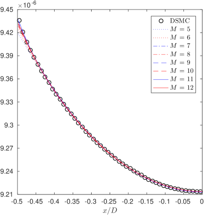
(a) Density, $\rho~{}({\rm kg\cdot m^{-3}})$

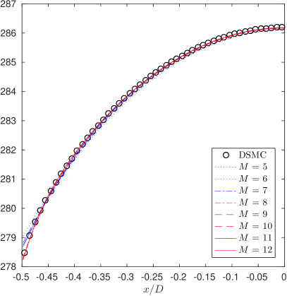
(b) Temperature, $T~{}({\rm K})$

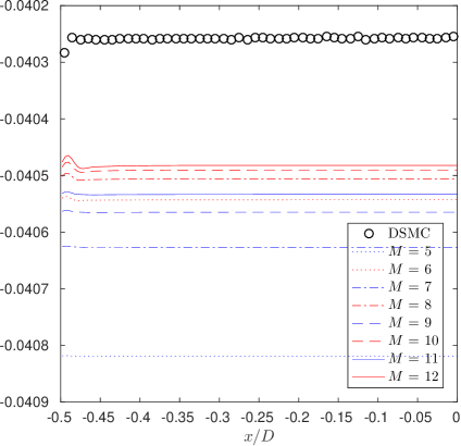
(c) Shear stress, $\sigma_{12}~{}({\rm kg\cdot m^{-1}\cdot s^{-2}})$

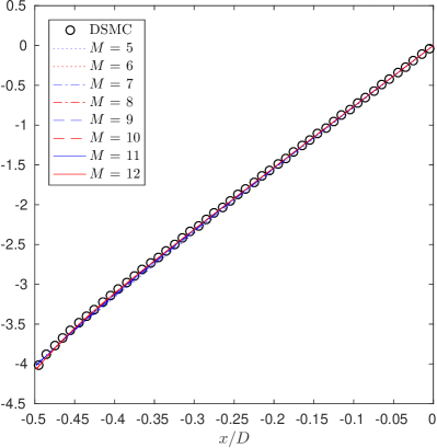
(d) Heat flux, $q_{1}~{}(\rm kg/s^{3})$

Figure 1: Solution of the Couette flow for the quadratic collision term (39) with $M_{0}=5$ and $D=0.092456{\rm m}$ ($\mathit{Kn}=0.1$).

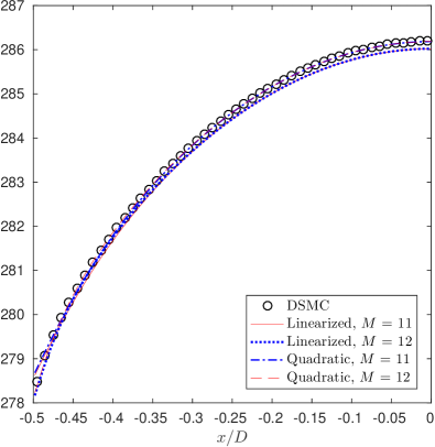
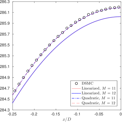
Figure 2: Comparison of temperature $({\rm K})$ profiles (left) and its zoom (right) between the quadratic collision term (39) and its linearization (52) with $M_{0}=5$ and $D=0.092456{\rm m}$ ($\mathit{Kn}=0.1$).

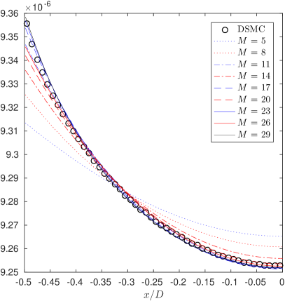
(a) Density, $\rho~{}({\rm kg\cdot m^{-3}})$

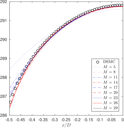
(b) Temperature, $T~{}({\rm K})$

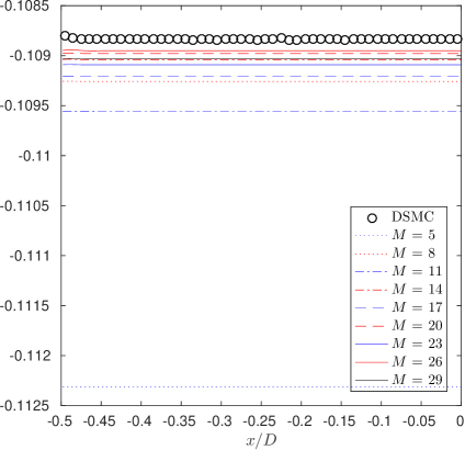
(c) Shear stress, $\sigma_{12}~{}({\rm kg\cdot m^{-1}\cdot s^{-2}})$

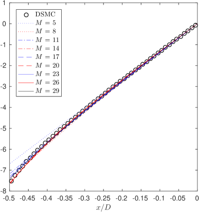
(d) Heat flux, $q_{1}~{}(\rm kg/s^{3})$

Figure 3: Solution of the Couette flow for the quadratic collision term (39) with $M_{0}=5$ and $D=0.018491{\rm m}$ ($\mathit{Kn}=0.5$).

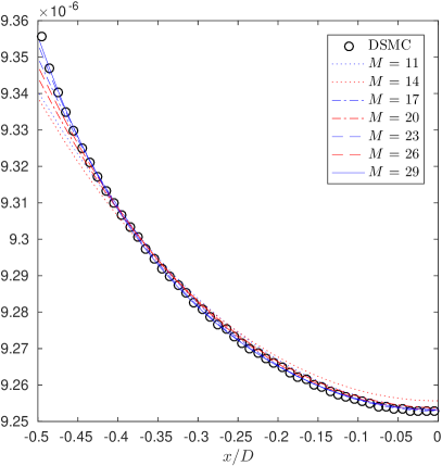
(a) Density, $\rho~{}({\rm kg\cdot m^{-3}})$

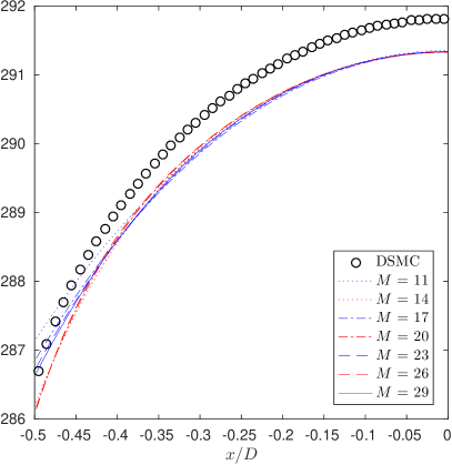
(b) Temperature, $T~{}({\rm K})$

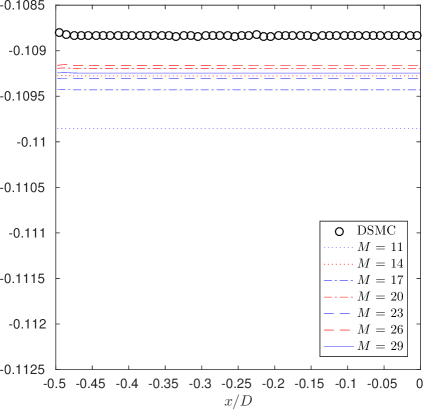
(c) Shear stress, $\sigma_{12}~{}({\rm kg\cdot m^{-1}\cdot s^{-2}})$

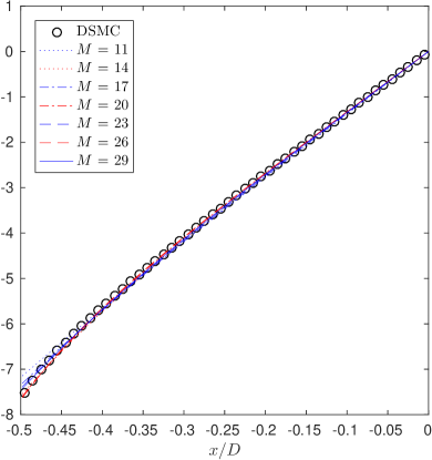
(d) Heat flux, $q_{1}~{}(\rm kg/s^{3})$

Figure 4: Solution of the Couette flow for the linearized collision term (52) with $M_{0}=10$ and $D=0.018491{\rm m}$ ($\mathit{Kn}=0.5$).

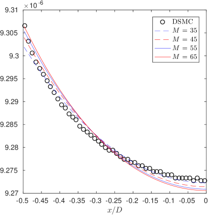
(a) Density, $\rho~{}({\rm kg\cdot m^{-3}})$

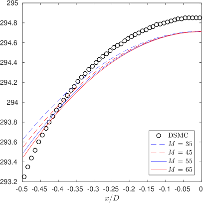
(b) Temperature, $T~{}({\rm K})$

(c) Shear stress, $\sigma_{12}~{}({\rm kg\cdot m^{-1}\cdot s^{-2}})$

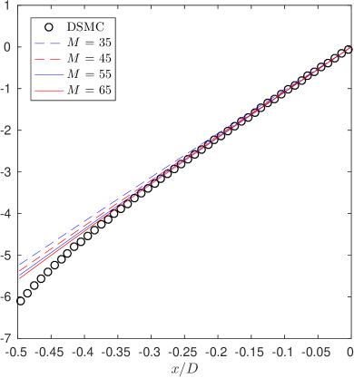
(d) Heat flux, $q_{1}~{}(\rm kg/s^{3})$

Figure 5: Solution of the Couette flow for the quadratic collision term (39) with $M_{0}=10$ and $D=0.003698{\rm m}$ ($\mathit{Kn}=2.5$).

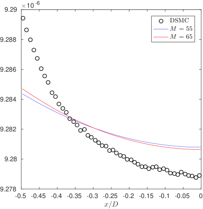
(a) Density, $\rho~{}({\rm kg\cdot m^{-3}})$

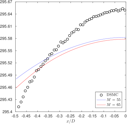
(b) Temperature, $T~{}({\rm K})$

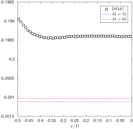
(c) Shear stress, $\sigma_{12}~{}({\rm kg\cdot m^{-1}\cdot s^{-2}})$

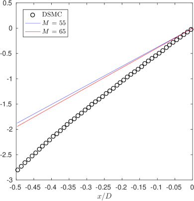
(d) Heat flux, $q_{1}~{}(\rm kg/s^{3})$

Figure 6: Solution of the Couette flow for the quadratic collision term (39) with $M_{0}=10$ and $D=0.00074{\rm m}$ ($\mathit{Kn}=12.5$).

5.2.2 The Fourier flow

The second benchmark problem is the Fourier flow which also studies the motion of the gas between two infinite parallel plates. In contrast to the planar Couette flow, both plates are stationary, while their temperature is different. Specifically, the left plate has the temperature $T_{l}^{w}=273.15{\rm K}$ and the right plate has the temperature $T_{r}^{w}=4T_{l}^{w}=1092.6{\rm K}$. In this situation, the gas also reaches a steady state as time goes. To simulate it, we adopt $\overline{\boldsymbol{u}}=0$ and $\overline{\theta}=\frac{k_{B}}{m}T_{r}^{w}$. The accommodation coefficient in the boundary condition is set to be $\omega=1$, and the computational domain is still $[-D/2,D/2]$ with $D$ being the distance between two plates. Four distances $D=0.092456{\rm m}$, $0.018491{\rm m}$, $D=0.003698{\rm m}$ and $0.00074{\rm m}$ with the corresponding dimensionless Knudsen number $\mathit{Kn}=0.1$, $0.5$, $2.5$ and $12.5$ respectively, are considered. Only results for quadratic collision term (39) are presented.

(1) $D=0.092456{\rm m}$, $\mathit{Kn}=0.1$: Numerical results for density $\rho$, temperature $T$, normal stress $\sigma_{11}$ and heat flux $q_{1}$ with $M_{0}=5$, together with the DSMC solutions, are shown in Figure 7. Our results coincide very well with the DSMC solutions for density and temperature, while a small deviation for normal stress $\sigma_{11}$ and heat flux $q_{1}$ can be observed. Note that for heat flux $q_{1}$, the relative deviation between the DSMC solution and our solution is less than $3\%$ for all $M$. It is worth mentioning that $q_{1}$ should be a constant in the steady-state solution, while the DSMC method provides a slanting profile. Such a result suggests the possible numerical error in the DSMC method, although we have run the DSMC code more than six days. It is left to the future work to determine what this constant should be.

Nevertheless, the deviation between our results and the DSMC solutions can be reduced by increasing $M_{0}$ in the collision term. As an example, we plot the results of normal stress $\sigma_{11}$ and heat flux $q_{1}$ with $M_{0}=10$ in Figure 8. Remarkable improvement can be observed.

(2) $D=0.018491{\rm m}$, $\mathit{Kn}=0.5$: Numerical results with $M_{0}=5$ and $M_{0}=10$, are presented in Figure 9 and 10, respectively. For this larger Knudsen number, evident deviations for all plotted quantities, in comparison to the DSMC results, can be observed even for a large $M$ in the case $M_{0}=5$. This indicates $M_{0}=5$ is not enough for the simulation in this case.

As shown in Figure 10, the results with $M_{0}=10$ again show considerable improvement, especially for $M$ which is odd and larger than $20$. For these $M$, all plotted quantities match the DSMC solutions quite well. It can also be observed that convergence of all plotted quantities with an even $M$ is much slower, especially in the region near the left plate. The underlying reason remains to be further studied.

(3) $D=0.003698{\rm m}$, $\mathit{Kn}=2.5$: Numerical solutions for $M_{0}=10$ in this case are given in Figure 11, which shows the results for $M=35,45,55,65$. Despite a large Knudsen number, for all quantities, the profiles for different $M$ are very close to each other, and they all agree well with DSMC solutions. The maximum relative deviation for all these quantities is less than $0.2\%$, which again shows the applicability of the Hermite spectral method for transitional flows.

(4) $D=0.00074{\rm m}$, $\mathit{Kn}=12.5$: Numerical results for density $\rho$, temperature $T$, normal stress $\sigma_{11}$ and heat flux $q_{1}$ with $M_{0}=10$, together with the DSMC solutions, are shown in Figure 12. It seems that our solutions are comparable with the DSMC solution for all these four quantities with $M=65$. The relative deviation between our solution and the DSMC solution for the density and the temperature is $1.2\%$ and $1.5\%$, respectively. But for the normal stress, the relative deviation is up to $15\%$. The relative deviation for heat flux is still quite small as to $0.1\%$. This may indicate the inadequacy of $M_{0}$ in this simulation.

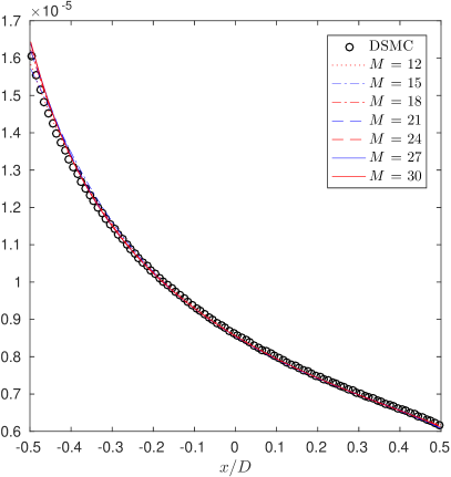
(a) Density, $\rho~{}({\rm kg\cdot m^{-3}})$

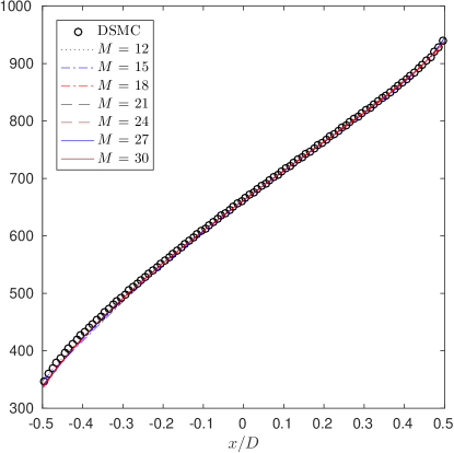
(b) Temperature, $T~{}({\rm K})$

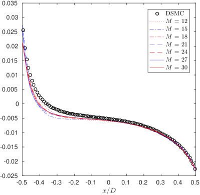
(c) Normal stress, $\sigma_{11}~{}({\rm kg\cdot m^{-1}\cdot s^{-2}})$

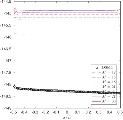
(d) Heat flux, $q_{1}~{}(\rm kg/s^{3})$

Figure 7: Solution of the Fourier flow for the quadratic collision term (39) with $M_{0}=5$ and $D=0.092456{\rm m}$ ($\mathit{Kn}=0.1$).

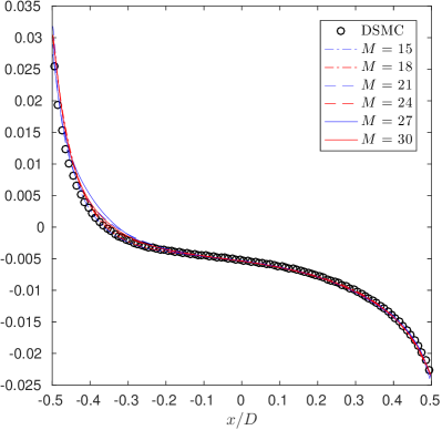
(a) Normal stress, $\sigma_{11}~{}({\rm kg\cdot m^{-1}\cdot s^{-2}})$

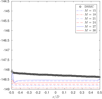
(b) Heat flux, $q_{1}~{}(\rm kg/s^{3})$

Figure 8: Normal stress and Heat flux of the Fourier flow for the quadratic collision term (39) with $M_{0}=10$ and $D=0.092456{\rm m}$ ($\mathit{Kn}=0.1$).

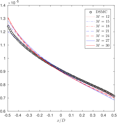
(a) Density, $\rho~{}({\rm kg\cdot m^{-3}})$

(b) Temperature, $T~{}({\rm K})$

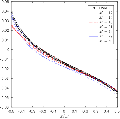
(c) Normal stress, $\sigma_{11}~{}({\rm kg\cdot m^{-1}\cdot s^{-2}})$

(d) Heat flux, $q_{1}~{}(\rm kg/s^{3})$

Figure 9: Solution of the Fourier flow for the quadratic collision term (39) with $M_{0}=5$ and $D=0.018491{\rm m}$ ($\mathit{Kn}=0.5$).

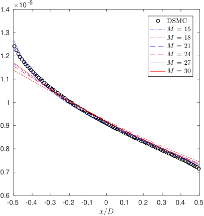
(a) Density, $\rho~{}({\rm kg\cdot m^{-3}})$

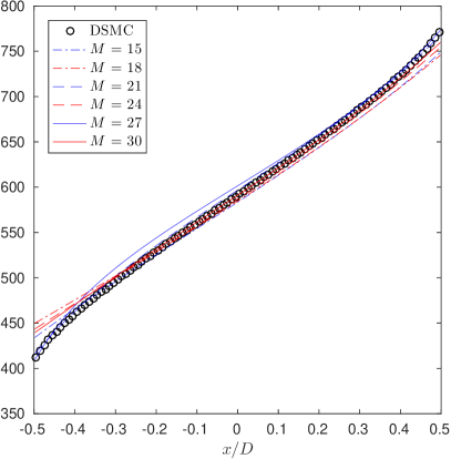
(b) Temperature, $T~{}({\rm K})$

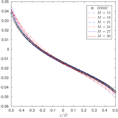
(c) Normal stress, $\sigma_{11}~{}({\rm kg\cdot m^{-1}\cdot s^{-2}})$

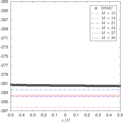
(d) Heat flux, $q_{1}~{}(\rm kg/s^{3})$

Figure 10: Solution of the Fourier flow for the quadratic collision term (39) with $M_{0}=10$ and $D=0.018491{\rm m}$ ($\mathit{Kn}=0.5$).

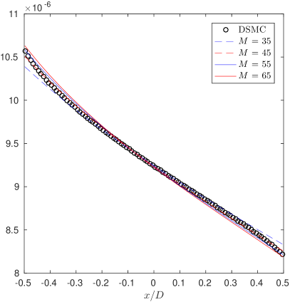
(a) Density, $\rho~{}({\rm kg\cdot m^{-3}})$

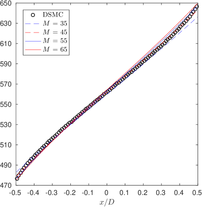
(b) Temperature, $T~{}({\rm K})$

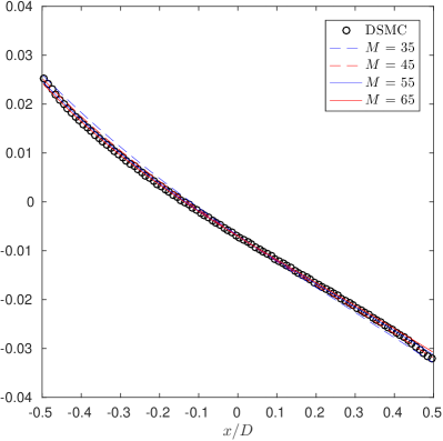
(c) Normal stress, $\sigma_{11}~{}({\rm kg\cdot m^{-1}\cdot s^{-2}})$

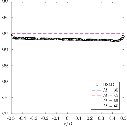
(d) Heat flux, $q_{1}~{}(\rm kg/s^{3})$

Figure 11: Solution of the Fourier flow for the quadratic collision term (39) with $M_{0}=10$ and $D=0.003698{\rm m}$ ($\mathit{Kn}=2.5$).

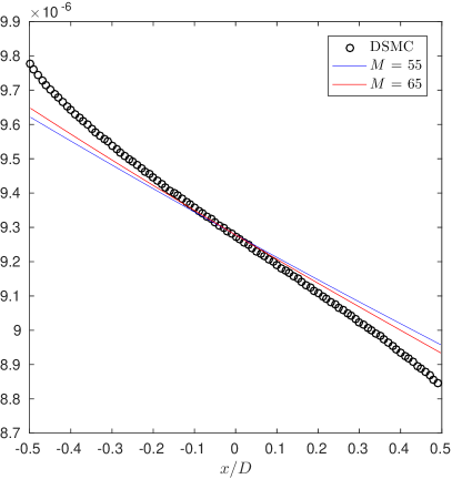
(a) Density, $\rho~{}({\rm kg\cdot m^{-3}})$

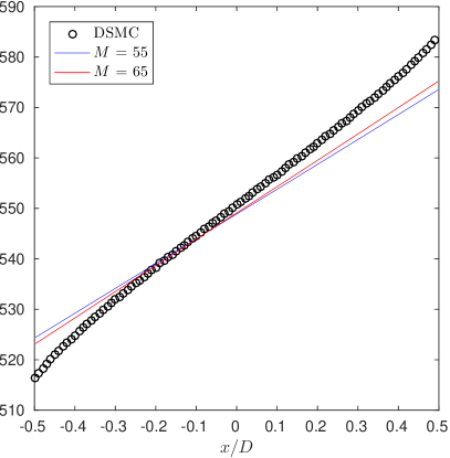
(b) Temperature, $T~{}({\rm K})$

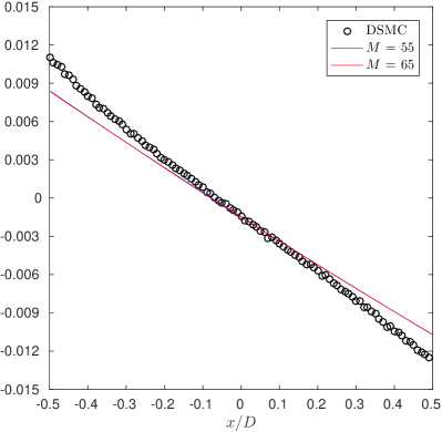
(c) Normal stress, $\sigma_{11}~{}({\rm kg\cdot m^{-1}\cdot s^{-2}})$

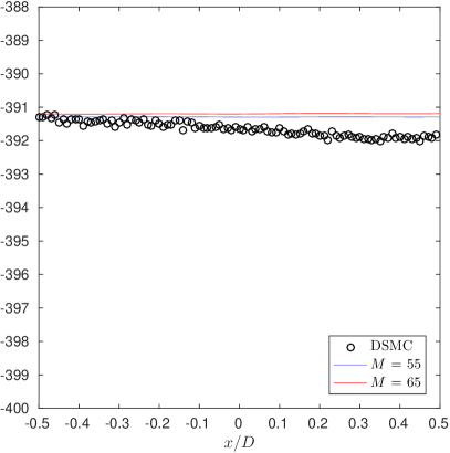
(d) Heat flux, $q_{1}~{}(\rm kg/s^{3})$

Figure 12: Solution of the Fourier flow for the quadratic collision term (39) with $M_{0}=10$ and $D=0.00074{\rm m}$ ($\mathit{Kn}=12.5$).

5.3 Two-dimensional numerical experiments

As a preliminary study of our method in the multi-dimensional case, we consider the two-dimensional lid-driven cavity flow which has been studied in [22, 30, 10]. In this case, the argon gas ($m=6.63\times 10^{-26}{\rm kg}$) is confined in a square cavity with side length $L=1.25\times 10^{-6}{\rm m}$. The temperature of the cavity walls is $T=T_{\mathrm{ref}}=273{\rm K}$. The viscosity coefficient $\mu$ is set to be

$$\mu=\mu_{\mathrm{ref}}\left(\frac{T}{T_{\mathrm{ref}}}\right)^{\frac{1}{2}(\eta+3)/(\eta-1)},$$

where the reference viscosity is $\mu_{\mathrm{ref}}=2.117\times 10^{-5}{\rm kg/(m\cdot s)}$, and the value of $\eta$ is $7.45$. Initially, the gas is in a uniform equilibrium with velocity $\boldsymbol{u}=0{\rm m/s}$ and temperature $T=273{\rm K}$, and the following two initial densities are considered:

1. $\rho=0.891{\rm kg/m^{3}}$, corresponding to Knudsen number $\mathit{Kn}=0.1$;

2. $\rho=0.0891{\rm kg/m^{3}}$, corresponding to Knudsen number $\mathit{Kn}=1.0$.

The gas flow is driven by the top lid of the cavity, which moves right at a constant speed $\boldsymbol{u}_{w}=(50,0,0){\rm m/s}$. We expect that the steady state can be after sufficiently long time. The simulation is carried out on a $100\times 100$ grid by explicit time stepping until $5.24\times 10^{-8}{\rm s}$. For both cases, we choose $M_{0}=10$, $\bar{\boldsymbol{u}}=0$ and $\overline{\theta}=\frac{k_{B}}{m}T_{\rm ref}$ in our numerical tests.

The simulation is run on the CPU model Intel Xeon E5-2680 v4 @ 2.40GHz, and 28 threads are used in the simulation. Details of the simulations are given in Table 1. Here the total CPU time is obtained by the C function clock(), whose result is the sum of CPU time for all threads. Inspired by the tables presented in [13], we also provide the CPU time for each time step, each spatial grid and each degree of freedom for easier comparison.

Table 1: Run-time data for the lid-driven cavity flow simulations

Test case	$\mathit{Kn}=0.1$	$\mathit{Kn}=1.0$
$M$	$25$	$35$
Number of coefficients ($N_{M}$)	$3276$	$8436$
Time step ($\Delta t$)	$2.64\times 10^{-12}{\rm s}$	$2.19\times 10^{-12}{\rm s}$
Number of time steps ($N_{s}$)	$19829$	$23968$
Total CPU time ($T_{\mathrm{total}}$)	$6.93\times 10^{6}{\rm s}$	$1.07\times 10^{7}{\rm s}$
CPU time per time step ($T_{s}=T_{\mathrm{total}}/N_{s}$)	$3.50\times 10^{2}{\rm s}$	$4.46\times 10^{2}{\rm s}$
CPU time per grid ($T_{g}=T_{s}/100^{2}$)	$3.50\times 10^{-2}{\rm s}$	$4.46\times 10^{-2}{\rm s}$
CPU time per degree of freedom ($T_{d}=T_{g}/N_{M}$)	$1.07\times 10^{-5}{\rm s}$	$5.30\times 10^{-6}{\rm s}$

The results are again compared with DSMC results [22], which are provided in Figure 13 and 14. In general, two results agree well with each other, while some discrepancy can be found on the boundary of the domain. Such discrepancy is probably related to the Gibbs phenomenon in the spectral method, since the distribution function on the boundary of the domain is generally discontinuous. Possible improvement includes using filters [1] or other boundary conditions [27], which will be part of our future work.

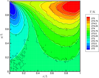
(a) Temperature

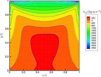
(b) Shear stress

Figure 13: Numerical results for $\mathit{Kn}=0.1$. White contours: Hermite spectral method. Black contours: DSMC.

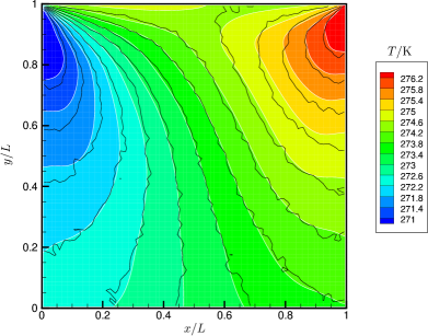
(a) Temperature

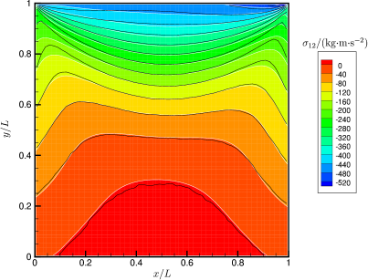
(b) Shear stress

Figure 14: Numerical results for $\mathit{Kn}=1.0$. White contours: Hermite spectral method. Black contours: DSMC.

6 Conclusion

Based on the Hermite spectral method, we have developed a numerical solver for the Boltzmann equation with an approximate collision operator proposed in [29]. The approximate collision operator is derived from the original quadratic collision operator, but the quadratic form is preserved only for the first few moments. Our numerical simulation shows that a small number of degrees of freedom for the quadratic part can already provide much better results than the linear models, which makes it possible to design numerical methods that can well balance the workload and the accuracy. Our major contribution to the algorithm is a special implementation of the collision operator. As is mentioned in Section 1, the implementation of such a special collision operator in the spatially inhomogeneous case is not as straightforward as for the spatially homogeneous and normalized equation considered in [29]. By introducing a fast algorithm to change basis functions, we eventually obtain a numerical scheme with time complexity $O(M_{0}^{9}+M^{4})$.

Such a numerical cost makes the algorithm highly promising when applied to more complicated problems. Research works on more multi-dimensional problems and polyatomic gases are ongoing.

References

- [1] J. Aguirre and J. Rivas, A spectral viscosity method based on Hermite functions for nonlinear conservation laws, SIAM J. Numer. Anal., 46 (2008), pp. 1060–1078.
- [2] G. A. Bird, Approach to translational equilibrium in a rigid sphere gas, Phys. Fluids, 6 (1963), pp. 1518–1519.
- [3] G. A. Bird, Molecular Gas Dynamics and the Direct Simulation of Gas Flows, Oxford: Clarendon Press, 1994.
- [4] Z. Cai, Y. Fan, and R. Li, A framework on moment model reduction for kinetic equation, SIAM J. Appl. Math., 75 (2015), pp. 2001–2023.
- [5] Z. Cai, Y. Fan, R. Li, and Z. Qiao, Dimension-reduced hyperbolic moment method for the Boltzmann equation with BGK-type collision, Commun. Comput. Phys., 15 (2014), pp. 1368–1406.
- [6] Z. Cai and R. Li, Numerical regularized moment method of arbitrary order for Boltzmann-BGK equation, SIAM J. Sci. Comput., 32 (2010), pp. 2875–2907.
- [7] Z. Cai, R. Li, and Z. Qiao, NR simulation of microflows with shakhov model, SIAM J. Sci. Comput., 34 (2012), pp. A339–A369.
- [8] Z. Cai, R. Li, and Z. Qiao, Globally hyperbolic regularized moment method with applications to microflow simulation, Computers and Fluids, 81 (2013), pp. 95–109.
- [9] Z. Cai and M. Torrilhon, Approximation of the linearized Boltzmann collision operator for hard-sphere and inverse-power-law models, J. Comput. Phys., 295 (2015), pp. 617–643.
- [10] Z. Cai and M. Torrilhon, Numerical simulation of microflows using moment methods with linearized collision operator, J. Sci. Comput., 74 (2018), pp. 336–374.
- [11] S. Chapman and T. G. Cowling, The Mathematical Theory of Non-uniform Gases, Third Edition, Cambridge University Press, 1990.
- [12] S. Chen, K. Xu, and Q. Cai, A comparison and unification of ellipsoidal statistical and Shakhov BGK models, Adv. Appl. Math. Mech., 7 (2015), pp. 245–266.
- [13] G. Dimarco, R. Loubére, J. Narski, and T. Rey, An efficient numerical method for solving the Boltzmann equation in multidimensions, J. Comput. Phys., 353 (2018), pp. 46–81.
- [14] I. M. Gamba, J. R. Haack, C. D. Hauck, and J. Hu, A fast spectral method for the Boltzmann collision operator with general collision kernels, SIAM J. Sci. Comput., 39 (2017), pp. B658–B674.
- [15] I. M. Gamba and S. Rjasanow, Galerkin-Petrov approach for the Boltzmann equation, J. Comput. Phys., 366 (2018), pp. 341–365.
- [16] D. Goldstein, B. Sturtevant, and J. E. Broadwell, Investigations of the motion of discrete-velocity gases, Progress in Astronautics and Aeronautics, 117 (1989), pp. 100–117.
- [17] H. Grad, On the kinetic theory of rarefied gases, Comm. Pure Appl. Math., 2 (1949), pp. 331–407.
- [18] A. Harten, P. D. Lax, and B. V. Leer, On upstream differencing and Godunov-type schemes for hyperbolic conservation laws, SIAM Review, 25 (1983), pp. 35–61.
- [19] Z. Hu and R. Li, A nonlinear multigrid steady-state solver for 1D microflow, Computers and Fluids, 103 (2014), pp. 193–203.
- [20] Z. Hu, R. Li, and Z. Qiao, Acceleration for microflow simulations of high-order moment models by using lower-order model correction, J. Comput. Phys., 327 (2016), pp. 225–244.
- [21] Z. Hu, R. Li, and Z. Qiao, Extended hydrodynamic models and multigrid solver of a silicon diode simulation, Commun. Comput. Phys., 20 (2016), pp. 551–582.
- [22] B. John, X.-J. Gu, and D. R. Emerson, Investigation of heat and mass transfer in a lid-driven cavity under nonequilibrium flow conditions, Numerical Heat Transfer, Part B: Fundamentals, 58 (2010), pp. 287–303.
- [23] J. C. Maxwell, On stresses in rarefied gases arising from inequalities of temperature, Proc. R. Soc. Lond., 27 (1878), pp. 304–308.
- [24] C. Mouhot and L. Pareschi, Fast algorithms for computing the Boltzmann collision operator, Math. Comp., 75 (2006), pp. 1833–1852.
- [25] A. V. Panferov and A. G. Heintz, A new consistent discrete-velocity model for the Boltzmann equation, Math. Method Appl. Sci., 25 (2002), pp. 571–593.
- [26] L. Pareschi and B. Perthame, A fourier spectral method for homogeneous Boltzmann equations, Transport Theor. Stat., 25 (1996), pp. 369–382.
- [27] N. Sarna and M. Torrilhon, On stable wall boundary conditions for the Hermite discretization of the linearised Boltzmann equation, J. Stat. Phys., 170 (2018), pp. 101–126.
- [28] W. Su, S. Lindsay, H. Liu, and L. Wu, Comparative study of the discrete velocity and lattice Boltzmann methods for rarefied gas flows through irregular channels, Phys. Rev. E, 96 (2017), p. 023309, https://doi.org/10.1103/PhysRevE.96.023309, https://link.aps.org/doi/10.1103/PhysRevE.96.023309.
- [29] Y. Wang and Z. Cai, Approximation of the Boltzmann collision operator based on Hermite spectral method, arXiv:1803.11191, (2018). submitted.
- [30] L. Wu, J. M. Reese, and Y. Zhang, Solving the Boltzmann equation deterministically by the fast spectral method: application to gas microflows, J. Fluid Mech., 746 (2014), pp. 53–84.