Relationships between HI Gas Mass, Stellar Mass and Star Formation Rate of HICAT+WISE (HI-WISE) Galaxies

Abstract

We have measured the relationships between Hi mass, stellar mass and star formation rate using the Hi Parkes All Sky-Survey Catalogue (HICAT) and the Wide-field Infrared Survey Explorer (WISE). Of the 3,513 HICAT sources, we find 3.4 $\upmu$m counterparts for 2,896 sources (80%) and provide new WISE matched aperture photometry for these galaxies. For our principal sample of spiral galaxies with $W1$ $\leq$ 10 mag and $z$ $\leq$ 0.01, we identify Hi detections for 93% of the sample. We measure lower Hi-stellar mass relationships that Hi selected samples that do not include spiral galaxies with little Hi gas. Our observations of the spiral sample show that Hi mass increases with stellar mass with a power-law index 0.35; however, this value is dependent on T-type, which affects both the median and the dispersion of Hi mass. We also observe an upper limit on the Hi gas fraction, which is consistent with a halo spin parameter model. We measure the star formation efficiency of spiral galaxies to be constant at $10^{-9.57}$ yr^-1 $\pm$ 0.4 dex for 2.5 orders of magnitude in stellar mass, despite the higher stellar mass spiral showing evidence of quenched star formation.

1 Introduction

Star formation is fueled by atomic (Hi) and molecular hydrogen, so we expect correlations between Hi mass, stellar mass and star formation rates (SFR). This is exemplified by the Kennicutt–Schmidt law that establishes a correlation between gas surface density and SFR, albeit both for Hi and molecular gas, and with considerable scatter (Kennicutt, 1998). Correlations are also observed between stellar mass and Hi mass (e.g., Catinella et al., 2010; Huang et al., 2012; Maddox et al., 2015), although these are partially explained by luminosity–luminosity correlations. However, the presence of mass quenching indicates that Hi mass declines above some high stellar mass threshold (e.g., Kauffmann et al., 2003; Gabor et al., 2010).

Although the relationship between Hi mass and SFR in a galaxy is predicted by the Kennicutt–Schmidt law, there is a scatter of $\sim$0.2 dex (Kennicutt, 1998), implying that Hi mass is just one of several factors that regulate SFR. Multiple studies using different surveys find that Hi mass ($M_{{H{\sc I}}}$) increases with SFR (Mirabel & Sanders, 1988; Doyle & Drinkwater, 2006). Hi disk is a precondition for star formation, but star formation also requires gas accretion from the intergalactic medium to drive the Hi gas inward, thereby cooling and converting it into molecular hydrogen (e.g., Prochaska & Wolfe, 2009; Obreschkow et al., 2016). By comparison, the relationship between molecular hydrogen and SFR is better understood since stars form in molecular clouds. Recent works (Leroy et al., 2008; Schruba et al., 2011) have shown that molecular hydrogen, rather than Hi, drives the Kennicutt–Schmidt law, but an empirical study on the relationship between molecular hydrogen and SFR using a large sample of galaxies is difficult to perform because of the lack of large-scale CO surveys. Also, there is uncertainty in converting CO intensity to molecular hydrogen content due to the uncertainty in the X-factor (Bolatto et al., 2013). Although Hi gas is only indirectly related to the SFR, the measurement of Hi gas can imply information about the molecular hydrogen of a galaxy (e.g., Leroy et al., 2008; Wong et al., 2016).

Multiple studies have found that Hi mass increases with stellar mass (Catinella et al., 2010; Huang et al., 2012; Maddox et al., 2015), which is partially explained by luminosity–luminosity correlations. However, the relations measured by different studies disagree with each other. Huang et al. (2012) find $\langle\log{}$ $M_{{H{\sc I}}}$$\rangle$ $\propto 0.712\langle\log{}$ $M_{\ast}$$\rangle$ for $M_{\ast}$$\leq$ 10⁹ ${\rm M_{\sun}}$ and $\langle\log{}$ $M_{{H{\sc I}}}$$\rangle$ $\propto 0.276\langle\log{}$ $M_{\ast}$$\rangle$ for $M_{\ast}$ $>$ 10⁹ ${\rm M_{\sun}}$. The break in the relationship represents the transition from irregular, low stellar mass galaxies to high mass, disk galaxies (Maddox et al., 2015; Kereš et al., 2009). However, Catinella et al. (2010) observed that Hi mass increases little with stellar mass (to the power of 0.02) for galaxies with $M_{\ast}$ $>$ 10⁹ ${\rm M_{\sun}}$.

The differences in the relation between Hi mass and stellar mass in the literature may be due to sample selection. The samples of Huang et al. (2012) and Maddox et al. (2015) use the Hi Arecibo Legacy Fast ALFA survey (ALFALFA) population, while the GASS sample of Catinella et al. (2010) is selected by stellar mass ($M_{\ast}$ $>10^{10}$ ${\rm M_{\sun}}$). By definition, the Hi selected samples of Huang et al. (2012) and Maddox et al. (2015) are more Hi-rich compared to a stellar mass-selected sample, and are biased against high stellar mass elliptical galaxies with very little Hi gas, resulting in elevated trends for Hi mass versus stellar masses. While the literature shows Hi mass increases with stellar mass, perhaps with a break or a plateau at high stellar masses (i.e., Catinella et al., 2010; Huang et al., 2012; Maddox et al., 2015), there are quantitative disagreements that we suspect are the result of sample selections.

How the Hi based star formation efficiency (SFE), or its inverse, the Hi depletion timescale (t_dep), varies with a galaxy’s stellar mass is unclear from the current literature. Huang et al. (2012), Jaskot et al. (2015), and Lutz et al. (2017) find that SFE increases with stellar mass for Hi selected samples. Therefore, low mass galaxies that are more Hi-rich than high stellar mass galaxies are inefficient at using their fuel reservoirs to form stars. Contradicting this, Schiminovich et al. (2010) find SFE of massive galaxies ($M_{\ast}$$>$ 10¹⁰ ${\rm M_{\sun}}$) to be constant at 10^-9.5 yr^-1, and Wong et al. (2016) find SFE to be constant at 10^-9.65 yr^-1 across 5 orders of magnitude of stellar mass for star-forming galaxies. Incompleteness and sample size are issues for relations from the prior literature, with Jaskot et al. (2015) having WISE detections for 63% of their Hi sources while Wong et al. (2016) is highly complete, but contains just 84 galaxies.

A key limitation of previous studies is low completeness, particularly for infrared counterparts for Hi sources, which facilitate the measurement of stellar masses and SFRs. Doyle & Drinkwater (2006) used fluxes from Infrared Astronomical Satellite (IRAS) to calculate SFRs for galaxies in the Hi Parkes All-Sky Survey (HIPASS) optical catalog, HOPCAT Doyle et al. (2005). Due to the $0.5^{\prime}$ angular resolution and 0.7 Jy 10-sigma sensitivity of IRAS at 12 ${\rm\upmu m}$, they only found infrared counterparts for 32% of the Hi Parkes All-Sky Survey catalog (HICAT). Their final sample comprised of galaxies with high SFRs and excluded galaxies with low rates of star formation, including elliptical galaxies and dwarf galaxies, because at $z$ $=$ 0.01, IRAS can only detect sources brighter than $\nu L_{\nu}$ $\sim 1\times 10^{10}$ ${\rm L_{\odot}}$. Jaskot et al. (2015) improved on previous studies by using WISE, which has a 12 ${\rm\upmu m}$ 5-sigma sensitivity of 1 mJy, but at the $z\sim 0.06$ maximum redshift of ALFALFA galaxies WISE detects galaxies brighter than $\nu L_{\nu}$ $\sim$ 6$\times 10^{8}$ ${\rm L_{\odot}}$, which resulted in Jaskot et al. (2015) finding infrared counterparts for just 63% of their Hi sources. To improve on the prior literature, we need large samples of galaxies that are highly complete for Hi counterparts, while probing large ranges of stellar mass, Hi mass, and SFR.

For this work, we measure the relationship between Hi mass, stellar mass, and SFR using three galaxy samples combining HICAT and WISE. The paper is arranged as follows: Section 2 describes data used in this research, Section 3 details the equations used to calculate the masses and SFRs, Section 4 describes the samples, Sections 5 and 6 present the results, Section 7 discuss the results and Section 8 summarizes our work. All magnitudes are in the Vega system. The cosmology applied in this paper is H₀ $=$ 70 km s^-1, $\Omega_{M}$ $=$ 0.3, and $\Omega_{\Lambda}$ $=$ 0.7.

2 Data

2.1 HICAT

The principal source of data for our analysis is the HICAT catalog, which is derived from the HIPASS survey (Barnes et al., 2001; Meyer et al., 2004). HIPASS is a blind survey below a declination $\delta$ of +2$\arcdeg$, performed with the Parkes 64-m radio telescope using a 21 cm multi-beam receiver. The HICAT catalog contains 4,315 Hi sources selected from HIPASS and is 99% complete at a peak flux of 84 mJy and an integrated flux of 9.4 Jy km s^-1 (Meyer et al., 2004; Zwaan et al., 2004).

For each Hi source in HICAT, we search for optical counterparts using the position and velocity measurements in the HICAT catalog. Since the HIPASS data has a spatial resolution of 15.5′, it is necessary to obtain more accurate positions for the Hi sources before searching for their mid-infrared counterparts in the WISE frames. To this end, we search for optical counterparts in the spectroscopic sample of Bonne et al. (2015), the NASA/IPAC Extragalactic Database (NED), HYPERLEDA (Makarov et al., 2014), and HOPCAT (Doyle et al., 2005). In order to accurately match the Hi sources with their optical counterparts, we cross-check the velocity measurements from HICAT with the velocity provided from the above sources for all possible positional matches. We describe each source below—as well as the matching process—in detail.

In our preliminary search for optical counterparts, we use the spectroscopic sample of Bonne et al. (2015), which covers the full survey area of HICAT and provides velocities (predominantly from the r_F $\leq$ 15.60 2MASS selected 6dF Galaxy Survey, 6dFGS; Jones et al., 2009), morphologies, and WISE photometry from the All-Sky public-release archive (Cutri et al., 2012) for 13,325 galaxies. For each source, we select the best match to this sample within 5′ and 400 km s^-1 of the respective HICAT position and velocity, resulting in 1,043 optical counterparts of 4,315 Hi sources.

To obtain additional optical counterparts, we then search in NED and HYPERLEDA for galaxies within 10′ and 400 km s^-1 of their respective HICAT positions and velocities. As NED and HYPERLEDA draw information from catalogs such as HICAT, it must be ensured that the velocities extracted from these databases are sourced from optical or high-resolution Hi radio observations and not sourced from HICAT, and hence that HICAT velocities are not being cross-matched to themselves.

HOPCAT (Doyle et al., 2005) is used as our last source for optical matches. The matches from HOPCAT can not be cross-checked with known velocities, but are categorized as ‘good guesses’ by Doyle et al. (2005) (see the reference for details on HOPCAT and its matching criteria). We do not use HOPCAT as our primary source for optical matches because Bonne et al. (2015), NED, and HYPERLEDA described above provide more recent velocity measurements from 6dFGS and other surveys that were not available at the time HOPCAT was compiled. The final number of galaxies taken from each source described here is listed in Table 1. In total, optical counterparts were obtained for 3,719 Hi sources. However, 147 of these were found to be multi-galaxy systems and were thus excluded from our analysis.

Table 1: The number of optical matches for HICAT.

	Number of sources
Total	4,315
No optical match	596
Position and velocity match	3,313
Position match	406
Bonne et al. (2015)	1043
NED and HYPERLEDA	2,270
HOPCAT	406

2.2 WISE Photometry

WISE was launched in December 2009, and mapped the entire sky in four mid-infrared bands: W1, W2, W3 and W4 (3.4 $\upmu$m, 4.6 $\upmu$m, 12 $\upmu$m, and 22 $\upmu$m; Wright et al., 2010). Once WISE depleted its cryogen in October 2010, it was then operated in a “warm” state using the two short bands and then placed in hibernation for well over 2 years. As part of the NEOWISE program, WISE was reactivated in September 2013 and continues to observe in the W1 and W2 bands (Mainzer et al., 2014). The point source sensitivities of W1, W2, W3 and W4 in Vega magnitudes are 16.5, 15.5, 11.2 and 7.9, respectively (Wright et al., 2010), in which W4 is approximately two orders of magnitude more sensitive than IRAS.

We have measured new WISE photometry for the optical counterparts of the HICAT source using the procedure described in Jarrett et al. (2013). We chose to do this because the profile-fit photometry data in the ALLWISE public-release archive (Cutri et al., 2012) of the (degraded resolution) mosaics is optimized for point sources (e.g., Jarrett et al., 2013; Cluver et al., 2014, and references therein). Therefore, resolved sources such as our sample galaxies are either measured as several point sources, or their flux is underestimated by the PSF photometry (mpro). The WISE default catalogs do include extended source photometry for 2MASS Extended Source Catalog (2MXSC; Jarrett et al., 2000) galaxies, but the elliptical apertures (gmag) misses a significant fraction of the flux (Cluver et al., 2014).

All measurements are carried out on WISE image mosaics that are constructed from single native frames using a drizzle technique (Jarrett et al., 2012), re-sampled with 1 sq. arc pixels (relative to a 6 arcsec FWHM beam). Photometry for each individual HIPASS galaxy, principally flux measurements and surface brightness characterizations, are conducted using the system developed by T.H Jarrett specifically for WISE data (Jarrett et al., 2013, see Section 3.6). The system estimates photometric errors from the formal components, including the sky background variance and the local sky level, instrumental signatures and the absolute calibration. The error model also takes into account the correlation between re-sampled pixels through a correction factor, which is detailed in the WISE Explanatory Supplement (see Section 2.3.f, Cutri et al., 2012). As detailed in Jarrett et al. (2013), the shape (inclination) and orientation were determined at a fixed $3\sigma$ isophotal level, which provides a robust and relatively accurate ($<$ 5%) estimate, although this assumes symmetry and a fixed shape to the 1-sigma edge of the galaxy.

As detailed in Jarrett et al. (2013, 2018, in prep), isophotal measurements at the W1 1-sigma level typically capture more than 96% of the total light for bulge-dominated galaxies, and to a lesser extent ($\geq$ 90%) for late-type galaxies, and most notably in the W3 and W4 bands as much as 20% of the light can be missing with low surface brightness galaxies. Hence, total fluxes are important in order to estimate the dust-obscured star formation activity in the W3 and W4 bands. The total flux is estimated by fitting a double Sersic function to the axisymmetric radial profile, consisting of an inner bulge and an outer disk. Integrating the composite Sersic model from the $1\sigma$ isophote to the edge of the galaxy (3 disk scale lengths) recovers the light that is below the single-pixel noise threshold; details of the fitting process in Jarrett et al. (2013). The error model for the total fluxes includes the goodness of fit, as well as the previous sky estimation per pixel estimates, and typically adds 4 to 5% to the isophotal flux uncertainty.

Lastly, each galaxy mosaic is visually inspected, and if necessary, bright stars and nearby galaxies are manually masked out, and the apertures are adjusted. Figure 1 compares our new WISE photometry for HICAT galaxies with the previously available archival fluxes and illustrates the impact of the new photometry on derived quantities. For example, for W1$\sim$12 mag galaxies our W1 and W3 magnitudes are on average systematically brighter by $\sim$ 1.4 mag and 1.1 mag than the default photometry pipeline magnitudes. Figure 2 shows four examples of the WISE mosaics that have been cleaned of neighboring objects, as well as the elliptical apertures used for photometry.

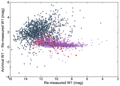
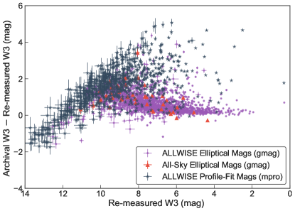
Figure 1: The difference between the archival and new magnitudes as a function of the new magnitude for W1 (top) and W3 (bottom). In order of preference, the archival data are either elliptical aperture magnitudes from the ALLWISE (purple) catalog or All-Sky magnitudes (navy) catalog, or PSF profile-fit (red) magnitudes from the ALLWISE catalog (Cutri & et al., 2013). For galaxies with W1$\sim$12 mag, the default elliptical aperture photometry is typically in error by $\sim$1 magnitude, while the PSF profile-fit photometry is in error by $\sim$2 magnitudes.

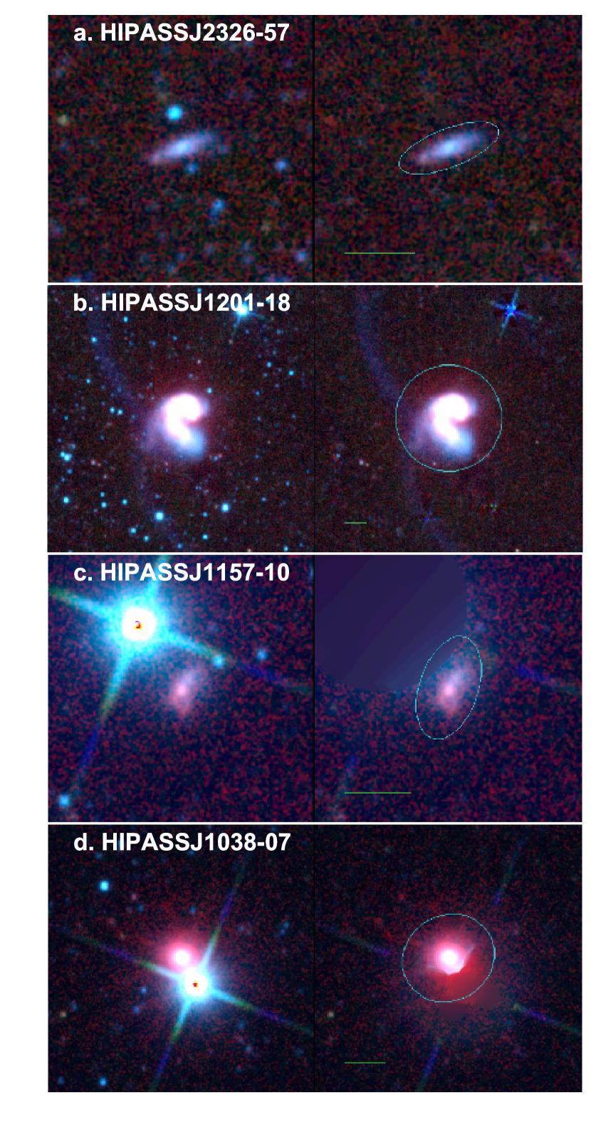
Figure 2: WISE color images image composed of W1, W2, W3, W4 bands of four Hi sources showing the galaxies before (left) and after (right) star and background source removal. The cyan ellipses indicate the $1\sigma$ apertures. The light from evolved stars are in blue and active star formation is in red. A scale of 2′ is indicated with the green horizontal line. North is upwards and East is to the left. HIPASSJ2326-57 is an example of a well behaved photometric galaxy; HIPASSJ1201-18 is a multi-galaxy Hi source; HIPASSJ1157-10 and HIPASSJ1038-07 are both flagged visually and have a W1 and W2 S/N $<$ 5 respectively.

We apply a S/N threshold of 5 in the W1 and W2 bands, a S/N threshold of 3 in the W3 band, and reject confused sources or Hi sources consisting of multiple galaxies. Consequently, we measure good W1-W2 photometry for 3,275 Hi sources and good W1-W2-W3 photometry for 2,831 Hi sources. We find 20 Hi sources that do not meet any of our WISE signal-to-noise thresholds and 147 Hi sources are multi-galaxy sources. From top to bottom, Figure 2 shows examples from HICAT of a “well behaved” source, a multi-galaxy source, and two visually flagged sources. A full list of parameters for HICAT+WISE (HI-WISE) is given in Table 8 in the Appendix. The 147 Hi sources that are found to be multi-galaxy systems are excluded from Table 8.

Figure 3 illustrates the WISE colors of HICAT galaxies, along with the expected colors of different types of galaxies, and clearly demonstrates that HIPASS is dominated by star-forming spiral galaxies, with relatively few ellipticals and luminous infrared galaxies (LIRGs). The galaxies with intermediate disk colors in AGN/LIRGs region may harbor dust-obscured AGNs and Seyferts (Jarrett et al., 2011; Huang et al., 2017).

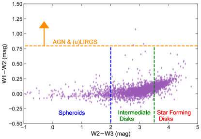
Figure 3: WISE mid-infrared colors of the HICAT sources with good WISE photometry. The horizontal and vertical lines denote the division between different types of galaxies (e.g., Jarrett et al., 2017). HICAT is dominated by star-forming, intermediate or late-type disk galaxies.

3 Stellar Mass, Hi Mass and Star Formation Rate Estimation

In this section, we will describe the methods used to estimate stellar mass, Hi mass and star formation rate (SFR) for our samples. For these quantities, we compiled distances from (in order of preference) Cosmicflows-3 (Tully et al., 2016) and HICAT. When distances are not available in the Cosmicflows-3 database, we determine luminosity distances using HIPASS redshifts by applying a Cosmic Microwave Background (CMB)-frame correction using the CMB dipole model presented by Fixsen et al. (1996), followed by an application of the LCDM. For samples selected by stellar mass (Sections 4.2 and 4.3), we include some galaxies that are not in HICAT, and for these galaxies, we use luminosity distances from velocities reported by NED in the same manner as stated above when distances are not available in the Cosmicflows-3 database. Table 8 lists these distances—and their respective sources—for each galaxy.

3.1 Stellar Mass

The W1 and W2 bands are dominated by light from K- and M-type giant stars, and thus trace the continuum emission from evolved stars with minimal extinction at low redshifts. Consequently, these bands are good tracers of the underlying stellar mass of a galaxy (Meidt et al., 2012; Cluver et al., 2014). However, the W2 band is also sensitive to hot dust, as well as 3.3 $\upmu$m polycyclic aromatic hydrocarbon (PAH) emission from extreme star formation and active galactic nuclei (AGN). W1 contains the 3.3 $\upmu$m PAH emission, but typically weak for normal star-forming galaxies (Ponomareva et al., 2018). As such, the aggregate stellar mass will be overestimated in the presence of an AGN (Jarrett et al., 2011; Stern et al., 2012; Meidt et al., 2014). In order to mitigate this problem, we exclude AGNs from our analysis that are identified in the AGN catalog of Véron-Cetty & Véron (2010).

Stellar masses were estimated following the GAMA-derived stellar mass-to-light ratio ($M_{\ast}/L_{\mathrm{W1}_{\mathrm{Sun}}}$) relation of Cluver et al. (2014):

$$\log_{10}M_{\ast}/L_{\mathrm{W1}_{\mathrm{Sun}}}=-1.96(\mathrm{W1}-\mathrm{W2})-0.03,$$ (1)

which depends on the “in-band” luminosity relative to the Sun,

$$L_{\mathrm{W1}_{\mathrm{Sun}}}=10^{-0.4(M-M_{\mathrm{Sun}})},$$ (2)

where $M$ is the absolute W1 magnitude and $M_{\mathrm{Sun}}$ $=$ 3.24 (Jarrett et al., 2013). Equation (1) was determined using Galaxy and Mass (GAMA; Driver et al., 2009) survey with stellar masses derived assuming a Chabrier (2003) IMF (Taylor et al., 2011; Cluver et al., 2014), and limited to galaxies with -0.05 $<$ W1$-$W2 $<$ 0.30, so we restrict the input colors for Equation (1) accordingly. The W1-W2 color dependence takes into account morphological dependence on the M/L and other factors, such as metallicity (Cluver et al., 2014). To determine the W1-W2 color, apertures are matched between the two bands. We typically use the W2 elliptical isophotal aperture as the fiducial since it is less sensitive than W1 and usually 10 to 15% smaller in radial extent. This is particularly the case for galaxies whose mid-infrared emission is dominated by stellar light (see Cluver et al., 2017; Jarrett et al., 2017).

The consistency of our stellar masses and those from other studies can be tested using MPA-JHU catalog (Brinchmann et al., 2004) for the Sloan Digital Sky Survey (SDSS; York et al., 2000). By construction, our WISE stellar masses agree with the SED stellar masses determined by GAMA (Driver et al., 2009; Taylor et al., 2011), with a $1\sigma$ scatter of just 0.2 dex, and the GAMA $M_{\ast}$$/L$ agree with the MPA-JHU $M_{\ast}$$/L$, with a bi-weight mean and $1\sigma$ scatter in the difference between $M_{\ast}$$/L$ of −0.01 and 0.07 dex. For dwarf galaxies the difference MPA-JHU between and UV-optical SED stellar masses (Huang et al., 2012) is zero with the objects lying within $\pm$0.35 dex ${\rm M_{\sun}}$(Maddox et al., 2015, and private correspondence). Thus, we do not expect large offsets between the stellar masses we have obtained from WISE and those which have been used by recent studies of Hi galaxies.

3.2 HI Mass

To calculate the Hi mass, we use the published integrated 21 cm flux ($F_{\textup{H{{i}}}}$) as follows:

$$\textup{M}_{\textup{H{{i}}}}[\textup{M}_{\sun}]=\frac{2.356\times 10^{5}}{1+z}\times D_{L}^{2}\times\textup{F}_{\textup{H{{i}}}}[\textup{Jy km s}^{-1}],$$ (3)

where $D_{L}$ is the luminosity distance to the galaxy in Mpc and $z$ is the redshift measured from the Hi spectrum (e.g., Lutz et al., 2017). The uncertainty in the Hi mass ($\Delta$$M_{{H{\sc I}}}$) is estimated using the method suggested by Doyle & Drinkwater (2006):

$$\Delta F_{\textup{H{{i}}}} =0.5\times F_{\textup{H{{i}}}}^{1/2},$$ (4)

$$\Delta\textup{M}_{\textup{H{{i}}}} =\textup{M}_{\textup{H{{i}}}}\frac{\Delta F_{\textup{H{{i}}}}}{F_{\textup{H{{i}}}}}.$$ (5)

3.3 Star Formation Rate

The W3 and W4 bands are sensitive to the interstellar medium, active galactic nuclei and star formation (e.g., Calzetti et al., 2007; Jarrett et al., 2011; Cluver et al., 2014, 2017). W4 emission is dominated by warm dust, and for star-forming galaxies W4 luminosity can be used to predict Balmer decrement correct H$\alpha$ luminosity with an accuracy of 0.2 dex (Brown et al., 2017). However, W4 lacks sensitivity and 39% of HICAT sources lack W4 detections.

WISE W3 luminosity includes contributions from PAHs, nebular emission lines, silicate absorption and warm dust, all of which are associated with star formation in galaxies. For $\sim L^{\ast}$ star-forming galaxies, Cluver et al. (2017) find PAHs and warm dust make 34% and 62.5% contributions, respectively, to the observed W3 luminosity. That said, we expect the contribution of PAHs to the W3 luminosity to decrease with decreasing galaxy mass due to the mass-metallicity relation of galaxies. Also, W3 better predicts the total infrared luminosity (and hence SFR) than W4 (Cluver et al., 2017). WISE W3 is thus a good star formation rate indicator, can be used to Balmer decrement corrected Ha luminosity with an accuracy of 0.28 dex (i.e., Brown et al., 2017).

Although the W3 band traces emission from star formation, it may also have contributions from evolved stellar populations. For $\sim L^{\ast}$ galaxies located at the centre of the star-forming main sequence, stellar continuum contributes 15.8% of the W3 light and we subtract from our data using the W1 photometry and the method of Helou et al. (2004). To account for this, we therefore scale the W1 integrated flux density, and subtract it from the W3 total flux to give an estimate of the W3 emission from the ISM, W3_PAH (Cluver et al., 2017). We use the prescription in Table 4 from Brown et al. (2017) to estimate the Balmer decrement corrected H$\alpha$ ($L_{H_{\alpha},\mathrm{Corr}}$):

$$\log{L_{W3_{\mathrm{PAH}}}}\;[\textup{erg s}^{-1}]= (40.79\pm 0.06)+(1.27\pm 0.04)\times$$

$$(\log{L_{H_{\alpha},\mathrm{Corr}}}\;[\textup{erg s}^{-1}]-40),$$ (6)

with a $1\sigma$ scatter of 0.28 dex. SFRs are estimated by scaling the Kennicutt (1998) calibration to a Chabrier (2003) IMF:

$$SFR\;[M_{\sun}\>\textup{yr}^{-1}]=(4.6\times 10^{-42})\times L_{H_{\alpha},\mathrm{Corr}}\;[\textup{erg s}^{-1}].$$ (7)

The uncertainty in SFR is dominated by the scatter in the relationship between WISE W3 luminosity and Balmer decrement corrected H$\alpha$ luminosity and therefore the uncertainty in log(SFR) $\sim$ 0.28 dex (Brown et al., 2017).

We use the SFR calibration from Brown et al. (2017) because it provides better SFR estimates for a broad range of galaxies—including LIRGs and blue compact dwarfs galaxies—compared to the prior literature. Also, Cluver et al. (2017) compared the SFR calibrations from the prior literature to their calibration derived from total infrared luminosity and found the SFR calibration from Brown et al. (2017) to agree with their own.

4 Samples

We create three samples to address specific science questions: an Hi selected sample (Hi sample), a stellar mass-selected sample (M_s sample) and a spiral sample. In addition to addressing specific science questions, these samples allow us to compare to the prior literature and to explore the impact that galaxy morphology and selection bias have on the scaling relationships between star formation, stellar mass, and Hi mass.

For the remainder of the paper we focus on galaxies (including 3,513 HICAT galaxies) that are at least 10 degrees away from the Galactic plane and are not known AGNs (from Véron-Cetty & Véron (2010) catalog), although we do include some additional galaxies in our summary of galaxy coordinates, redshifts, and photometry provided in Table 8. We also exclude objects north of the main HICAT footprint ($\delta$ $\geq$ $+2$) from the M_s sample and spiral sample.

4.1 Hi Selected Sample

We use the Hi Parkes All-Sky Survey catalog (HICAT) to form the basis of the Hi selected sample. Out of 3,513 HICAT sources, 2,826 have good W1 and W2 photometry. Of these, 2,396 also have good photometry for the W3 band, and 2,342 galaxies in this category have significant W3_PAH flux (W3 flux with the stellar continuum subtracted). Figure 4 shows the percentage of Hi sources with WISE counterparts as a function of Hi mass. We achieve a HICAT-WISE match completeness of 80% for Hi mass $>$ 10^9.5 ${\rm M_{\sun}}$.

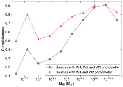
Figure 4: The fraction of HICAT sources with WISE photometry, compared to the total sample, as a function of Hi mass. Out of 3,513 HICAT sources, 80% have good W1 and W2 detections and 68% have good W3 detections.

4.2 Spiral Sample

To measure the distribution of Hi masses and SFRs as a function of stellar mass and morphology, we generate a stellar mass-selected sample of spiral galaxies (the spiral sample). The spiral sample is drawn from the Bonne et al. (2015) catalog, which achieves a 99% completeness in redshifts and morphologies for galaxies with $K_{\mathrm{tot}}$ $<$ 10.75. We maximize Hi completeness by limiting the sample to spiral galaxies (defined with de Vaucouleurs T-type $\geq$ 0) with redshift $\leq$ 0.01 and re-measured W1 magnitude $<$ 10. Our spiral sample consists of 600 galaxies.

For 435 of our spiral galaxies we obtained Hi fluxes from HICAT, while for a further 121 galaxies we obtained archival Hi fluxes from Paturel et al. (2003), Huchtmeier & Richter (1989), Springob et al. (2005) and Masters et al. (2014). The details of the Hi counterparts are provided in Table 2. As we illustrate in Figure 5, 93% of the spiral galaxies have Hi detections.

Table 2: The number of galaxies the spiral sample and the M_s sample with Hi counterparts.

Hi Source	Spiral Sample	Ms sample
Total	600	839
HICAT	435	454
Paturel et al. (2003)	100	114
Huchtmeier & Richter (1989)	13	13
Springob et al. (2005)	1	2
Masters et al. (2014)	7	7

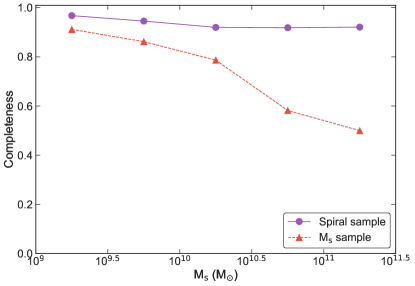
Figure 5: The fraction of galaxies in the spiral sample and the M_s sample with Hi mass measurements. For the spiral sample, 556 out of 600 galaxies have a Hi counterpart, giving the spiral sample a completeness of 93%. 590 galaxies out of the 839 galaxies in the M_s sample have a Hi counterpart.

The aforementioned W1 and redshift limits are chosen because of the brightness limitation of the parent sample and the detection sensitivity of HICAT. While the notional limit for the Bonne et al. (2015) is $K_{tot}$ $\leq$ 10.75, this limits the $W1$ $\leq$ 11.5 and galaxy numbers decline at $W1$ $>$10. Table 3 lists the number of galaxies in our sample, the number with HI detections and the percentage with HI detections with and without the redshift and W1 magnitude limits applied. Removing the redshift and magnitude limits from the spiral sample decreases the percentage of galaxies with HI detections to 50%, but has little impact on measured relations we describe in Section 5.

Table 3: The basic properties of our spiral sample and spiral galaxy samples without the redshift and W1 selection criteria applied.

	Spiral Sample	No W1-mag cut	No redshift cut	No W1 magnitude and redshift cuts applied
Total $\#$ of galaxies	600	792	1442	3458
$\#$ Hi counterparts	556	672	1048	1697
% with HI counterpart	93%	87%	73%	50%

4.3 Stellar Mass-selected Sample (M_s sample)

In order to compare the Hi mass, stellar mass and SFR relationships of this work to those of GASS (Catinella et al., 2010, 2012, 2013), which uses a stellar mass-selected sample, we have also produced such a sample (M_s sample). The GASS sample is designed to measure the neutral hydrogen content of 1000 galaxies to investigate the physical mechanisms that regulate how cold gas responds to different physical conditions in the galaxy and the processes responsible for the transition between star-forming spirals and passive ellipticals (Catinella et al., 2010).

The M_s sample selection is identical to that of the spiral sample except that it lacks the T-type criterion. The M_s sample contains 839 galaxies, of which 590 have an Hi counterpart. The details of the Hi counterparts are provided in Table 2. Figure 5 shows that the fraction of galaxies with an Hi measurement drops at the higher stellar masses, where the number of Hi-poor ellipticals increases.

5 $M_{{H{\sc I}}}$ - $M_{\ast}$ relationship

In this section, we will look at the relationship between Hi mass and stellar mass for all three samples. The Hi–stellar mass relation is one of the principal means used to provide insight to the history of gas accretion and star formation. Also, as discussed in Section 7, it can be used to test models of the stability of Hi disks and how these disks can fuel star formation (Wong et al., 2016; Obreschkow et al., 2016). For each sample, we bin the data into stellar mass bins with a width of $\log$($M_{\ast}$) $=$ 0.5 and for bins with $\geq$ 10 galaxies we measure the median Hi mass and $1\sigma$ scatter in Hi mass for each stellar mass bin. The $1\sigma$ scatter about the median is determined using the range encompassing 68% of the data. For the spiral sample and M_s sample, care is needed when accounting for the galaxies with Hi non-detections. When estimating the median Hi mass as a function of the stellar mass, we assume the Hi upper limits are below the median Hi mass for the relevant stellar mass bin, which is a reasonable approximation when the Hi detection rate is $\gg$ 50%. The median Hi masses are determined for any stellar mass bin with 10 or more galaxies and Hi detection rate above 50%. Upper limits for individual galaxies are determined using the integrated flux of 7.5 Jy km s^-1, corresponding to the HICAT’s 95% completeness limit (Zwaan et al., 2004).

While we list the individual uncertainties in Table 8, we find that W1 $\sim$ 12 galaxies have a stellar mass uncertainty $\leq$ 0.2 dex, and this uncertainty decreases with increasing W1 flux. Also, 80% of the Hi sample has an Hi mass uncertainty better than 20%.

5.1 HI Sample

The relationship between Hi mass and stellar mass for the Hi selected sample is illustrated in Figure 6. The Hi mass is a strong function of stellar mass among the Hi sample (Spearman’s rank correlation, $r_{s}$, $=$ 0.64) and the least-squares fit to the medians, represented by an orange line in Figure 6, is

$$\log{\;M_{\textup{H{\sc i}}}}=0.51\>(\log{\;M_{\ast}}-10)+9.71.$$ (8)

We fit 68% of the Hi masses are within 0.5 dex of our best-fit relation.

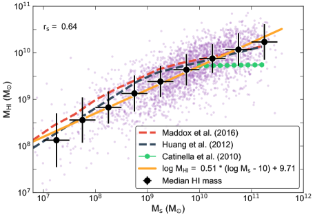
Figure 6: Hi mass versus stellar mass of the Hi selected sample. Spearman’s rank correlation, $r_{s}$, is listed in the top left corner. Our median Hi masses are slightly below those derived by Huang et al. (blue dashed-line; 2012), and Maddox et al. (red dashed-line; 2015), who both used ALFALFA Hi selected samples. However the Hi mass medians of the Hi sample are higher than the GASS sample (green solid-line; Catinella et al., 2010), which is a stellar mass-selected sample. Hi samples overestimate Hi mass as a function of stellar mass because Hi samples do not detect galaxies with low Hi mass, such as ellipticals.

Hi mass versus stellar mass relations for the Hi selected sample and previous studies (Catinella et al., 2010; Huang et al., 2012; Maddox et al., 2015) are also plotted in Figure 6. Our sample and the ALFALFA samples of Huang et al. (2012) and (Maddox et al., 2015) are Hi selected, while the GASS sample of Catinella et al. (2010) is stellar mass-selected. We find the relations for the Hi selected samples are qualitatively similar, with median Hi mass increasing with stellar mass. In contrast, the Hi versus stellar mass relation measured with the GASS sample (Catinella et al., 2010) is up to 0.5 dex lower than those derived from Hi selected samples, as the GASS sample includes galaxies with low Hi masses (including ellipticals). There are also discrepancies in the Hi versus stellar mass relations measured with different Hi selected samples. We do not see the break in the relation at a stellar mass of 10⁹ ${\rm M_{\sun}}$ that was previously observed by ALFALFA (i.e., Huang et al., 2012; Maddox et al., 2015). Below a mass of 10⁹ ${\rm M_{\sun}}$ our sample is less than 70% complete for WISE counterparts, and thus we may not be reliably measuring HI mass versus stellar mass in this mass range However, even if this was not an issue we believe this sample would produce a biased relation, as it (by construction) excludes galaxies that have high stellar masses but low HI masses (i.e., many elliptical galaxies).

5.2 Spiral Sample

The Hi and stellar mass distribution for the spiral sample is shown in Figure 7. The median Hi mass increases with stellar mass with a least-squared fit of

$$\log{\;M_{\textup{H{\sc i}}}}=0.35\>(\log{\;M_{\ast}}-10)+9.45,$$ (9)

with 68% of the Hi masses within 0.4 dex.

However, as Figure 7 illustrates, at a given stellar mass the median Hi mass increases with T-Type while the dispersion decreases with T-Type. For example, for the 10¹⁰ to 10^10.5 ${\rm M_{\sun}}$ stellar mass bin, the median Hi mass and the $1\sigma$ spread of galaxies for all spirals is 10^9.53 ${\rm M_{\sun}}$ $\pm$ 0.47 dex, for T-type 0 to 2 is 10^9.26 ${\rm M_{\sun}}$ $\pm$ 0.59 dex, and for T-type 6 to 8 is 10^9.72 ${\rm M_{\sun}}$ $\pm$ 0.31 dex. The increasing spread of HI masses with decreasing T-type for spiral galaxies may be part of a broader trend, as Serra et al. (2012) concluded that the HI mass distribution for early-type galaxies was far broader than that for spirals. They suggest this scatter reflects the large variety of Hi content of early-type galaxies, and confirms the lack of correlation between Hi mass and luminosity.

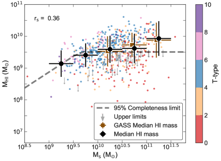
Figure 7: Hi mass versus stellar mass for the (highly complete) spiral sample. Symbols are color coded by morphology, the median HI masses are shown for the spiral sample (black circles) and the GASS sample (brown squares; Catinella et al., 2010). The dashed line shows the Hi mass limit for $z$ $\leq$ 0.01 and $W1$ $\leq$ 10 star-forming galaxies. The Spearman’s rank correlation coefficient is shown in the the top left. Hi mass is a function of both T-type and stellar mass. The median Hi masses increases with stellar mass with a power-law index of 0.35.

In Figure 7, we compare our Hi mass-stellar mass distribution of our spiral sample to that from GASS (Catinella et al., 2010), using GASS galaxies that we have classified as spirals with Galaxy Zoo 1 (GZ1; Lintott et al., 2011). Using the GZ1 classifications and a 70% vote threshold, we find GASS comprises 305 spirals, 273 elliptical and 182 galaxies with uncertain morphology. We repeat our analysis on the GASS sample, using the same stellar mass bins and Hi median mass calculations with stellar mass bins with 10 or more galaxies and an Hi detection rate $>$ 50%. The estimated median Hi masses for the spiral sample, and the GASS spiral samples are listed in Table 4. The median Hi masses for the GASS spiral sample increases with stellar mass similar to our spiral sample. The median Hi mass of the spiral samples differs about 0.08 dex on average. To explain the relationship between Hi mass and stellar mass of the spiral samples we turn to the halo spin parameter models of Obreschkow et al. (2016) in Section 7.

Table 4: Median Hi mass and $1\sigma$ (68%) scatter as a function of stellar mass for the spiral sample, and the GASS spiral sample.

	Spiral Sample				GASS Spiral Sample
log($M_{\ast}$)	log($M_{{H{\sc I}}}$)	$1\sigma$	Total	% Hi	log($M_{{H{\sc I}}}$)	$1\sigma$	Total	% Hi
(${\rm M_{\sun}}$)	(${\rm M_{\sun}}$)	(${\rm M_{\sun}}$)		Detections	(${\rm M_{\sun}}$)	(${\rm M_{\sun}}$)		Detections
9.25	9.14	0.42	31	97
9.75	9.41	0.37	129	95
10.25	9.59	0.43	225	92	9.53	0.47	130	89
10.75	9.61	0.46	174	97	9.73	0.38	111	94
11.25	9.93	0.54	38	92	9.88	0.55	64	83

5.3 M_s Sample

In Figure 8, we present Hi mass versus stellar mass for our M_s sample and the equivalent stellar mass-selected sample of GASS (Catinella et al., 2010). The estimated median Hi masses of the M_s sample and the GASS sample are listed in Table 5. For the M_s sample the Hi mass increases with the stellar mass for the stellar mass bins $\leq$ 10^10.5 $M_{\ast}$ and then flattens for the highest stellar mass bin. The estimated Hi mass median for the highest stellar mass bin may be underestimated, as the Hi completeness for this bin is only 58% and our assumption that all non-detections are below the median could be in error.

At stellar masses greater than 10¹⁰ ${\rm M_{\sun}}$, median Hi mass is almost constant with stellar mass, and our measurements agree with those of GASS to within 0.3 dex. This is in contrast with the trend shown in Figure 7 for the spiral sample. The obvious explanation, given the prior literature (e.g., Catinella et al., 2010; Huang et al., 2012), is that this is due to the increasing fraction of gas poor early-type galaxies at high $M_{\ast}$, as illustrated in the top panel of Figure 8. Serra et al. (2012) found that early-type galaxies host less Hi than spiral galaxies, but have a broader range of Hi masses. For example, Serra et al. (2012) find that elliptical galaxies have Hi mass from 10⁷ to 10⁹ ${\rm M_{\sun}}$(the lower limit is uncertain as this overlooks Hi non-detections in their sample), while the Hi mass distribution for spirals peaks at $\sim$ 2$\times$ 10⁹ ${\rm M_{\sun}}$, with a small number of galaxies below 10⁸ ${\rm M_{\sun}}$. Combining this result with our previous findings from our spiral sample, we conclude that as one moves from early-type to late-type galaxies, median HI mass increases while the scatter in HI mass decreases. Within an individual T-type, Hi mass typically increases with stellar mass, and it is the increasing fraction of early-types with increasing stellar mass that explains the roughly constant median Hi masses measured for the M_s sample.

Table 5: Median Hi mass and $1\sigma$ (68%) scatter as a function of stellar mass for the M_s sample, and the GASS sample.

	Ms sample				GASS Spiral Sample
log($M_{\ast}$)	log($M_{{H{\sc I}}}$)	$1\sigma$	Total	% Hi	log($M_{{H{\sc I}}}$)	$1\sigma$	Total	% Hi
(${\rm M_{\sun}}$)	(${\rm M_{\sun}}$)	(${\rm M_{\sun}}$)		Detections	(${\rm M_{\sun}}$)	(${\rm M_{\sun}}$)		Detections
9.25	9.10	0.50	34	91
9.75	9.56	0.27	145	86
10.25	9.48	0.41	272	79	9.14	0.64	299	68
10.75	9.03	0.89	299	58	9.32	0.62	292	63
11.25			84	50			168	50

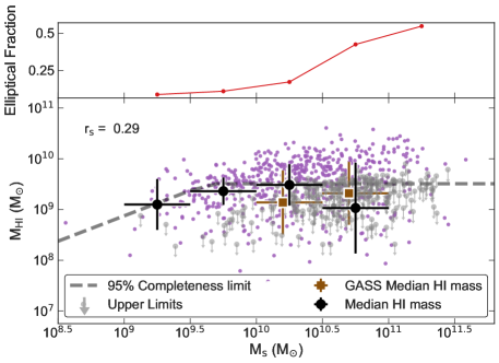
Figure 8: The spiral fraction versus stellar mass (upper panel) and Hi mass versus stellar mass (lower panel) for the M_s sample. Median HI masses are shown for the M_s sample (black circles) and the GASS sample (brown squares; Catinella et al., 2010). The HIPASS mass limit for galaxies at $z$ $\leq$ 0.01 and $W1$ $\leq$ 10 is shown by the gray dashed line and the Spearman’s rank correlation coefficient is shown in the top left. Hi mass is almost flat with increasing stellar mass for both samples, in large part because of the increasing fraction of passive early-type galaxies with increasing stellar mass.

5.4 The Impact of Sample Selection

A key conclusion from the previous sections is sample selection impacts measured Hi mass versus stellar mass relations, and to illustrate this in Figure 9 we plot Hi mass–stellar mass relations for Hi selected samples, spiral galaxy samples and stellar mass selected samples, including data from both our work and the literature. For all values of stellar mass, Hi selected samples have a higher Hi mass than spiral-selected and stellar mass-selected samples. This is because Hi surveys are designed to sample a large number of Hi-rich systems, and therefore lack the sensitivity to detect the Hi-poor galaxy population. For example, the HIPASS survey can detect galaxies with Hi masses $>$ 10⁹ ${\rm M_{\sun}}$ at $z$ $=$ 0.01; however, elliptical galaxies have Hi masses $\leq$ 10⁹ ${\rm M_{\sun}}$ (Serra et al., 2012), and would thus be largely missing from HIPASS samples at these redshifts. Even late-type galaxies in Figure 7 have HI masses as low as 10⁸ ${\rm M_{\sun}}$, and thus some are missing from HIPASS selected samples at $z$ $>$ 0.01. Similar selection effects apply to ALFALFA, albeit at higher redshifts. This is not surprising and indeed was a motivation for studies such as GASS, but does illustrate that Hi mass versus stellar mass relations have a strong dependence on sample selection.

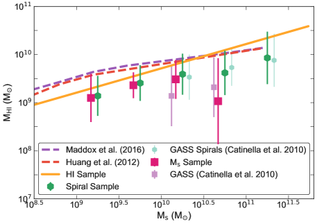
Figure 9: Comparison of HI mass versus stellar mass for our Hi selected sample, the spiral sample, the M_s sample (without morphological criteria) and the prior literature. Hi selected samples give consistently higher relations than the other samples, as (by definition) they exclude galaxies with comparatively low Hi masses.

6 Star-Forming Properties of the Spiral Sample

6.1 Star-forming Main Sequence

While the relationship between SFR and Hi mass is the principal focus of the paper, we are also able to measure the local ($z\leq 0.01$) star-forming main sequence (MS; e.g., Noeske et al., 2007; Rodighiero et al., 2011; Wuyts et al., 2011) using the spiral sample. Measurements of the MS are enhanced by our highly complete sample, our new WISE photometry (which should mitigate aperture bias—see Section 2.2), and our ability to take advantage of a recent calibration of W3 as a SFR indicator that uses large aperture photometry (Brown et al., 2017).

In Figure 10 we present our star-forming main sequence. As expected, the median of the $\log$ $SFR$ increases from -0.50 dex for the $10^{9}$ to 10^9.5 ${\rm M_{\sun}}$ stellar mass bin to 0.14 dex for the 10¹⁰ to 10^10.5 stellar mass bin, with the scatter of individual galaxies about the median being $\sim$ 0.3 dex. For stellar mass bins above 10¹⁰ ${\rm M_{\sun}}$, the median $\log$ $SFR$ is roughly constant at 0.14 while the scatter of the individual galaxy SFRs about the median increases from 0.38 to 0.49 dex. The changing trend of SFR with increasing stellar mass and the increased dispersion of SFRs is evidence of mass quenching (Kauffmann et al., 2003), and this also coincides with an increasing fraction of early-type spirals (T-type $\leq$ 2). To mitigate the effect of mass-quenching on our model fit to MS, we only fit to galaxies with stellar mass $\leq$ 10^10.5 ${\rm M_{\sun}}$(shown in Figure 10b) and measure the MS to be

$$\log{\;\mathrm{SFR}}=0.7\>(\log{\;M_{\ast}}-10)-0.09$$ (10)

with a $1\sigma$ scatter of 0.27 dex. Alternate selection criteria to mitigate the effect of mass-quenching produces similar MS fits. For example, a subsample of galaxies with T-type $>$ 2 produces a fit of $\log SFR=0.61(\log M_{\ast}-10)-0.08$ ($1s\sigma$ scatter $=$ 0.26 dex).

Figure 10b and Table 6 also compare the MS relation from this work to the prior literature (Zahid et al., 2012; Oliver et al., 2010; Chen et al., 2009; Elbaz et al., 2007; Salim et al., 2007; Grootes et al., 2013), with data taken from the extensive review by Speagle et al. (2014). To shift the Speagle et al. (2014) homogenized MS relations from a Kroupa to Chabrier IMF, we apply a -0.03 and -0.07 dex shifts to the stellar masses and SFRs respectively. The blue line is the $z$ $=$ 0.01 MS relation given by Equation (28) from Speagle et al. (2014), and the shaded region is the “true” scatter about the MS (for more details, please refer to Speagle et al., 2014). The normalization (at $\log$ $M_{\ast}$ $=$ 10) of our best fit is 0.04 dex smaller and the slope is 0.21 larger than the best fit for the MS of Speagle et al. (2014). Speagle et al. (2014) note that the wide range for MS slopes for the local universe suggests that the systematics involved are underestimated, and they estimate the magnitude of these systematics on the MS slopes to be of the order of $\sim$0.2 dex. As we noted earlier, our slope does depend on the criterion used to reject galaxies that could be undergoing quenching, and including early-type spiral galaxies with masses above 10^10.5 ${\rm M_{\sun}}$ reduces our slope to 0.416 ($1\sigma$ scatter $=$ 0.34), which is closer to that of Speagle et al. (2014).

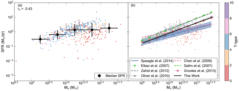
Figure 10: SFR versus stellar mass for the spiral sample with symbols color coded by morphology. The median SFRs are also shown in panel (a). The median SFR increases with stellar mass for $M_{\ast}$ $<$ 10^10.5 ${\rm M_{\sun}}$ and then flattens for $M_{\ast}$ $>$ $10^{10.5}$ ${\rm M_{\sun}}$, indicating evidence of mass quenching. To mitigate the effect of mass quenching, we model the MS using spiral galaxies with $M_{\ast}$ $<$ $10^{10.5}$ ${\rm M_{\sun}}$ and find $\log$ $SFR$ $=$ 0.7 $\times$ ($\log$ $M_{\ast}$$-$ 10) $-$ 0.09. As illustrated by panel (b), z$\sim$0.01 relations compiled by Speagle et al. (2014) show considerable scatter, and this may result (in part) from how studies exclude (or include) high mass spirals that may have already commenced quenching.

Table 6: Main-sequence relationships

Paper	$\alpha$	$\beta$	$\log$ $SFR(10)$	$z_{\mathrm{med}}$	$z_{\mathrm{range}}$	log $M_{\ast}$ range	Survey
This Study	0.7	-7.09	-0.09		$\leq$ 0.01	9.0-11.0	WISE
Zahid et al. (2012)	0.71$\pm$0.01	-6.78$\pm$0.1	0.32	0.07	0.04-0.1	8.5–10.4	SDSS
Oliver et al. (2010)	0.77$\pm$0.02	-7.88$\pm$0.22	-0.18	0.1	0.0-0.2	9.1–11.6	SWIRE
Chen et al. (2009)	0.35$\pm$0.09	-3.56$\pm$0.87	-0.06	0.11	0.005-0.22	9.0–12.0	SDSS
Elbaz et al. (2007)	0.77	-7.44	0.26	0.06	0.015-0.1	9.1-11.2	SDSS
Salim et al. (2007)	0.65	-6.33	0.17	0.11	0.005-0.22	9.0-11.1	GALEX-SDSS selected
Speagle et al. (2014)	0.49	-5.13	-0.03
Grootes et al. (2013)	0.550	-5.520	-0.02		$\leq$ 0.13	9.5-11	GAMA/Herschel-ALTAS
Cluver et al. (2017)	1.05$\pm$0.09	-10.40$\pm$0.88	0.09		z $<$ 0.01($<$ 30 Mpc)	7-11.5	SINGS/KINGFISH

6.2 Star Formation Efficiency

Star formation efficiency (SFE), defined as SFR/$M_{{H{\sc I}}}$, quantifies the current rate of gas consumption, dividing the SFR by Hi mass and SFE is expected to depend on the stellar mass of a galaxy (Schiminovich et al., 2010; Huang et al., 2012; Wong et al., 2016; Lutz et al., 2017). SFE and its inverse, the depletion time, have thus been commonly used to quantify gas consumption and test models of the stability of the galactic disks (e.g. Wong et al., 2016).

To investigate the relationship between star formation and Hi mass within the spiral sample, we plot in Figure 11 SFE as a function of stellar mass. In Table 7 we provide the median SFEs as a function of stellar mass, with the upper limits on the Hi mass being used for the Hi non-detections. The SFE remains relatively constant at a median SFE $=$ 10^-9.57 yr^-1, with a $1\sigma$ scatter of 0.44 dex for spiral galaxies with stellar masses between 10^9.0 and 10^11.5 ${\rm M_{\sun}}$. While we see evidence for mass quenching in high stellar mass spirals in Figure 10, the SFE appears to be constant for spiral galaxies falling on the MS and spiral galaxies that have (potentially) commenced quenching.

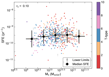
Figure 11: The SFE and the stellar mass for the spiral sample. Median SFEs for each stellar mass bin are estimated including the Hi mass upper limits for non-Hi detections, and the SFE medians and $1\sigma$ values are listed in Table 7. For stellar masses ranging from 10⁹ to 10^11.5 ${\rm M_{\sun}}$, the SFE for spirals remains constant at a median value of $\log\;\mathrm{SFE}=-9.57$ and $1\sigma$ spread of $0.4$ dex. SFE appears to be almost constant with T-type and stellar mass, despite the fact high mass galaxies with T-type$<$2 fall below the MS and may have commenced quenching.

SFE versus stellar mass relations for both the spiral sample and previous studies (Schiminovich et al., 2010; Jaskot et al., 2015; Wong et al., 2016; Lutz et al., 2017) are compared in Figure 12a. Hi selected samples (Jaskot et al., 2015; Lutz et al., 2017) exhibit an increasing SFE with stellar mass, however this reflects their selection bias against galaxies with low Hi masses. By contrast, stellar mass-selected samples (Schiminovich et al., 2010; Wong et al., 2016) find that SFE is constant with stellar mass; however, previous studies have measured differing values of this constant, ranging from 10^-9.65 yr^-1 (Wong et al., 2016) to 10^-9.5 yr^-1 (Schiminovich et al., 2010). Wong et al. (2016) provide two theoretically motivated relations for SFE versus stellar mass, which are both plotted in Figure 12b. The first relation assumes that the molecular gas fraction depends only on the stellar surface mass density, while the second assumes that this fraction depends on the hydrostatic pressure. Between stellar masses of 10^9.0 and 10^11.5 ${\rm M_{\sun}}$, the hydrostatic pressure model of Wong et al. (2016) (which gives a constant SFE) shows the greatest consistency with our work and other stellar mass-selected samples.

Table 7: The median SFE and 1$\sigma$ values of each stellar mass bin for the spiral sample shown in Figure 11.

log($M_{\ast}$)	Median log(SFE)	1$\sigma$	N
(${\rm M_{\sun}}$)	(yr-1)	(dex)
9.25	-9.72	0.51	29
9.75	-9.58	0.43	128
10.25	-9.49	0.41	222
10.75	-9.48	0.47	164
11.25	-9.56	0.39	35

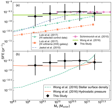
Figure 12: The median SFE and stellar mass for the spiral sample, alongside scaling relations observed in the prior literature (i.e., Schiminovich et al., 2010; Huang et al., 2012; Wong et al., 2016; Lutz et al., 2017) (panel a) and two models presented by Wong et al. (2016) (panel b). Hi selected samples find that SFE increases with stellar mass, but this is an artifact of excluding low Hi mass galaxies. Stellar mass-selected samples, on the other hand, find that SFE is constant with stellar mass, with normalization between 10^-9.65 yr^-1 to 10^-9.5 yr^-1. Of the two models presented by Wong et al. (2016), the hydrostatic pressure model provides the best agreement with our data.

7 Discussion

7.1 Is There an Upper Limit to the $M_{{H{\sc I}}}$?

For the spiral sample, we find that Hi mass increases with stellar mass, from 10^9.14 ${\rm M_{\sun}}$ at a stellar mass of 10^9.25 ${\rm M_{\sun}}$ to 10^9.93 ${\rm M_{\sun}}$ at a stellar mass of 10^11.25 ${\rm M_{\sun}}$ (see Figure 7). We also observe a stellar mass-dependent upper limit on Hi mass. In this section, we discuss the reason for this upper limit.

Both our Hi and stellar mass-selected samples imply an upper limit for Hi mass as a function of stellar mass, and such thresholds are also seen in prior literature (e.g., Maddox et al., 2015). Is this upper limit for Hi mass expected from theory? Maddox et al. (2015) argue that the maximum Hi fraction for galaxies with stellar masses $>$ 10⁹ ${\rm M_{\sun}}$ is set by the upper limit in the halo spin parameter, $\lambda$. The halo spin parameter is defined as

$$\lambda\equiv J_{\mathrm{halo}}E_{\mathrm{halo}}^{1/2}G^{-1}M_{\mathrm{halo}}^{-5/2},$$ (11)

where $J_{\mathrm{halo}}$ is the galaxy halo’s angular momentum, $E_{\mathrm{halo}}$ its total energy, and $M_{\mathrm{halo}}$ its total mass (Boissier & Prantzos, 2000). Maddox et al. (2015) determine the halo spin parameter of the ALFALFA galaxies and find that at a fixed stellar mass, the galaxies with the largest Hi mass also have the largest halo spin parameter (see their Figure 6). The large halo spin of a galaxy stabilizes the high Hi mass disk, preventing it from collapsing and forming stars.

Maddox et al. (2015) also measure the largest spin parameter to be $\lambda$ $\sim$ 0.2, confirming the upper limit on the halo spin parameter predicted by numerical $N$-body simulations of cold dark matter (Knebe & Power, 2008). They conclude that the upper limit on Hi fraction is set by the upper limit of the halo spin parameter due to the empirical correlation between the halo spin parameter and the Hi fraction.

Obreschkow et al. (2016) finds that for isolated local disk galaxies the fraction of atomic gas, $f_{\mathrm{atm}}$, is described by a stability model for flat exponential disks. To see if the observed upper limit to the Hi fraction of the spiral sample can be explained by the upper limit of the halo spin parameter, we calculate the $f_{\mathrm{atm}}$ relationship for $\lambda$ $\approx$ 0.112, following the method outlined in Obreschkow et al. (2016). Though $\lambda$ $\sim$ 0.2 is the maximum spin of a spherical halo, we choose to calculate the $f_{\mathrm{atm}}$ at $\lambda$ $\approx$ 0.112 because 99% of galaxy halos are predicted to lie below $\lesssim$ 0.112 (Bullock et al., 2001). We define the fraction of atomic gas as

$$f_{\mathrm{atm}}=\frac{1.35M_{H{\sc I}}}{M},$$ (12)

where M is the disk baryonic mass ($M$ $=$ $M_{\ast}$$+$ 1.35$M_{H{\sc I}}$) and the factor of 1.35 accounts for the universal helium fraction (Obreschkow et al., 2016). Obreschkow et al. (2016) models the rotation curve of spiral galaxies as

$$f_{\mathrm{atm}}=\min\left\{1,2.5q^{1.12}\right\},$$ (13)

where $q$ is the global stability parameter. This parameter is defined as:

$$q=\frac{j\sigma}{GM}=0.22\frac{\lambda}{0.03}\left(\frac{M}{10^{9}M_{\odot}}\right)^{-1/3},$$ (14)

where $j$ is the baryonic specific angular momentum of the disk, $\sigma$ is the velocity dispersion of the atomic gas and mass is in units of 10⁹ ${\rm M_{\sun}}$. The global stability parameter is simplified by making two assumptions: firstly, that disk galaxies condense out of scale-free cold dark matter halos, and secondly, that $j$ $\propto$ $\lambda$ (Obreschkow & Glazebrook, 2014; Obreschkow et al., 2016). Under these assumptions, Equation (13) simplifies to:

$$f_{\mathrm{atm}}=\min\left\{1,0.5\left(\frac{\lambda}{0.03}\right)^{1.12}\left(\frac{M}{10^{9}M_{\odot}}\right)^{-0.37}\right\},$$ (15)

and using Equation (12), this can be rearranged to give:

$$\frac{M_{H{\sc I}}}{10^{9}M_{\odot}}=\min\Biggl{\{} \frac{M}{1.35\times 10^{9}M_{\odot}},$$

$$18\lambda^{1.12}\left(\frac{M}{10^{9}M_{\odot}}\right)^{-0.63}\Biggr{\}}.$$ (16)

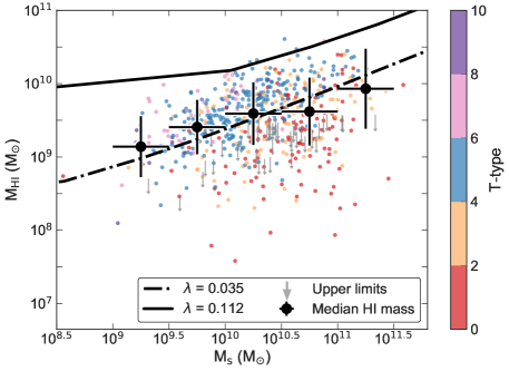
Figure 13: Hi mass versus stellar mass for the spiral sample. The solid and dashed black lines represent the model, Equation (7.1), for when $\lambda$ $=$ 0.112 and 0.035, respectively. The median bins of the spiral sample are in good agreement with the model of Obreschkow et al. (2016), as they lie on the expected mean $f_{\mathrm{atm}}$ (for $\lambda$ $=$ 0.035). The upper Hi masses of the spiral sample line up with the expected $f_{\mathrm{atm}}$ for $\lambda$ $=$ 0.112, and therefore the maximum Hi mass for a given stellar mass is determined by the upper limit in the halo spin parameter.

Figure 13 illustrates the comparison between Equation (7.1) and the empirical Hi–stellar mass distribution of the spiral sample. We also include the predicted $f_{\mathrm{atm}}$ curve for $\lambda$ $\approx$ 0.03, as this value of $\lambda$ corresponds to the mode of the empirically measured halo spin parameter distribution (Bullock et al., 2001). The median bins of the spiral sample are in agreement with this prediction of $f_{\mathrm{atm}}$, while the highest Hi mass galaxies lie below the predicted upper limit for $f_{\mathrm{atm}}$, when $\lambda=0.112$. We find that the model of Obreschkow et al. (2016) matches well with the empirical data of the spiral sample, consistent with the hypothesis that the upper limit of the Hi fraction is set by that of the halo spin parameter.

7.2 Why is SFE Constant?

We find that star formation efficiency is constant across two orders of magnitude of stellar mass, which agrees with the findings of Catinella et al. (2010) and Wong et al. (2016), while disagreeing with others (e.g., Huang et al., 2012; Lutz et al., 2017). Wong et al. (2016) tested two models for molecular gas content within galaxies: one where molecular gas is a function of stellar surface density and another where it is a function of hydrostatic pressure. The stellar surface density prescription (Leroy et al., 2008; Zheng et al., 2013) defines the molecular-to-atomic ratio, $R_{\mathrm{mol}}$, as

$$R_{\mathrm{mol},s}=\frac{\Sigma_{\ast}}{81M_{\odot}\,\mathrm{pc}^{-1}},$$ (17)

where $\Sigma_{\ast}$ is the stellar surface density. The $R_{\mathrm{mol}}$ for the hydrostatic pressure prescription (Zheng et al., 2013) is defined as

$$R_{\mathrm{mol},p}=\left(\frac{P_{h}}{1.7\times 10^{4}\,\mathrm{cm}^{-3}\,\mathrm{K}\,k_{B}}\right)^{0.8},$$ (18)

where $P_{h}$ is the hydrostatic pressure (Elmegreen, 1989) and $k_{B}$ is the Boltzmann constant.

Similarly to Wong et al. (2016), we find that the constant SFE can be described by a model of the marginally stable disk, while the hydrostatic pressure model provides a better prescription for estimating the SFE and molecular-to-atomic ratio. For massive galaxies with large optical disks, previous studies (e.g., Leroy et al., 2008; Wong et al., 2013) observed a correlation between $R_{\mathrm{mol}}$ and stellar surface density. The two models given by Equations (17) and (18) also predict similar $R_{\mathrm{mol}}$ and integrated SFE for high mass galaxies (Wong et al., 2016). But for low mass galaxies, the stellar surface density prescription does not predict the observed SFE because this prescription is unable to convert the Hi to molecular hydrogen, and underestimates the amount of molecular hydrogen in regions with low stellar surface densities. Therefore, this method underestimates the SFR and SFE in dwarf galaxies. While the stellar surface density model predicts that SFE will decrease for smaller stellar mass galaxies, the hydrostatic pressure model predicts a higher molecular hydrogen content for low mass galaxies, and therefore a constant SFE with stellar mass, agreeing with the empirical data.

We note that Obreschkow et al. (2016) predict that most of the baryons in dwarf galaxies are in the form of Hi gas ($f_{\mathrm{atm}}$ $=$ 1) and therefore have low SFE because these systems are inefficient at converting their Hi gas to molecular gas. We do not observe a decrease in SFE because these galaxies are below the stellar mass range probed in our spiral sample. Our lowest stellar mass bin of 10^9.0 and 10^9.5 ${\rm M_{\sun}}$ hints at a turn-over for the low mass dwarf, as predicted by Obreschkow et al. (2016). Combining the next generation of Hi survey, WALLABY, with 20-cm radio continuum from ASKAP, we will measure the Hi properties and SFR of $\sim$ 600,000 galaxies, including a large number of dwarf galaxies populating the low mass end of Figure 12. Observing these low stellar mass dwarfs will provide a more complete picture about Hi content and how efficiently dwarfs convert Hi to molecular gas.

8 Summary

We have measured the relationship between Hi mass, stellar mass and SFE using HICAT, archival Hi data and new WISE photometry. For this work, we provide new WISE aperture photometry for 3,831 out of 4,315 sources of HICAT and created three samples, an Hi selected sample, a spiral sample and a M_s sample. We find the following:

1. Sample selection and biases are critical when interpreting and comparing measured relationships between Hi mass, stellar mass and SFE. Hi selected samples often exclude Hi poor galaxies (unlike stellar mass selected samples) resulting in measurements of high median Hi masses and low median SFEs.

2. Hi mass increases with stellar mass for the spiral sample with a power-law index of 0.34. Also, at a given stellar mass, Hi mass increases with T-type and dispersion in Hi masses narrows for individual T-types. For example, for the $10^{10}$ ${\rm M_{\sun}}$ to $10^{10.5}$ ${\rm M_{\sun}}$ stellar mass bin, the median Hi mass and scatter is $10^{9.26}$ ${\rm M_{\sun}}$ and 0.59 dex for T-types 0 to 2 and the $10^{9.72}$ ${\rm M_{\sun}}$ and 0.31 dex for T-types 6 to 8.

3. Hi mass is constant with stellar mass for the M_s sample. While Hi mass increases with stellar mass for spiral galaxies, the fraction of elliptical galaxies with little Hi gas also increases with stellar mass, producing the observed flat relation.

4. The observed upper limit to the Hi-stellar mass distribution of the spiral sample is consistent with the predicted Hi-stellar mass curve for the upper limit for the halo spin parameter ($\lambda$ $=$ 0.112). This is consistent with the hypothesis the maximum Hi fraction is set by that of the halo spin parameter.

5. For a subsample of the spiral sample with stellar mass $\leq$ $10^{10.5}$ ${\rm M_{\sun}}$, we measure the MS to be $\log SFR=0.7(\log M_{\ast}-10)-0.09$ with a $1\sigma$ scatter of 0.27 dex. We see evidence of mass quenching (e.g. Kauffmann et al., 2003) as the median SFR is constant for spiral galaxies with stellar masses $>$ $10^{10}$ ${\rm M_{\sun}}$.

6. For the spiral sample, SFE is constant ($=$ $10^{-9.57}$ $\pm$ 0.44 yr^-1) for 2.5 orders of magnitude in stellar mass and agrees with comparable measurements of stellar mass selected samples of galaxies (Catinella et al., 2010; Schiminovich et al., 2010). This results is in broad agreement with the hydrostatic pressure model (Wong et al., 2016).

7. SFE is constant as a function of T-type and is constant for spiral galaxies that show evidence of mass quenching.

Table 8: HI-WISE parameter descriptions

Parameter	Units	Description
Name		HIPASS designation
RA	deg	Right ascension (J2000)
Dec	deg	Declination (J2000)
T-type		The T-type of galaxies reported by Bonne et al. (2015) or NED.
Dist	Mpc	Luminosity distance
Dist Source Flag		Source of the distance : 0. Cosmicflows-3 (Tully et al., 2016), 1. HICAT, 2. NED
Optical Match Type		Our category matching choice: 0. no optical counterpart, 1. position and velocity match, 2. position match.
velHI	km s-1	The flux weighted velocity average between minimum and maximum profile velocity.
$S_{\rm p}$	Jy	peak flux density of profile
$S_{\rm int}$	Jy km s-1	integrated flux of source (within region $v_{\rm lo}$, $v_{\rm hi}$ and box size)
W1	mag	W1 isophotal magnitude
W1err	mag	W1 magnitude error
W2	mag	W2 isophotal magnitude
W2err	mag	W2 magnitude error
W3	mag	W3 ‘best’ magnitude
W3err	mag	W3 magnitude error
W3f		W3 ‘best’ photometry type: 0. isophotal, 10. total magnitude
W4	mag	W4 ‘best’ magnitude
W4err	mag	W4 magnitude error
W4f		W4 ‘best’ photometry type: 0. isophotal, 10. total magnitude
R1iso	arcsec	W1 1-sigma isophotal radius (semi-major axis)
R2iso	arcsec	W2 1-sigma isophotal radius or photometry aperture (semi-major axis)
R3iso	arcsec	W3 1-sigma isophotal radius or photometry aperture (semi-major axis)
R4iso	arcsec	W4 1-sigma isophotal radius or photometry aperture (semi-major axis)
ba		axis ratio based on the W1 3-sigma isophote
pa	deg	position angle (east of north) based on the W1 3-sigma isophote
W1W2	mag	W1-W2 color, where the W1 aperture is matched to the W2 1-$\sigma$ isophotal aperture
W1W2err	mag	W1-W2 color uncertainty
W2W3	mag	W2-W3 color, using the W2 isophotal aperture and the W3 isophotal aperture
W2W3err	mag	W2-W3 color uncertainty
W1-W2	mag	K-corrected (rest-frame) W1-W2 color
W2-W3	mag	K-corrected (rest-frame) W2-W3 color
log $L_{W1}$	log L⊙	W1 $\nu L_{\nu}$ luminosity (log10)
log $L_{W1}$ err	log L⊙	uncertainty in log $L_{W1}$
log $L_{W2}$	log L⊙	W2 $\nu L_{\nu}$ luminosity (log10)
log $L_{W2}$ err	log L⊙	uncertainty in log $L_{W2}$
log $L_{W3}$	log L⊙	W3 $\nu L_{\nu}$ luminosity (log10). This includes the stellar continuum.
log $L_{W3}$ err	log L⊙	uncertainty in log $L_{W3}$
log $L_{W4}$	log L⊙	W4 $\nu L_{\nu}$ luminosity (log10).This includes the stellar continuum.
log $L_{W4}$ err	log L⊙	uncertainty in log $L_{W4}$
log $L_{W1}(L_{\odot})$	log L⊙	W1 in-band luminosity (log10)
log $L_{W1}(L_{\odot})$ err	log L⊙	uncertainty in log $L_{W1}(L_{\odot})$
W1flux	mJy	WISE W1 K-corrected flux
W2flux	mJy	WISE W2 K-corrected flux
w3PaH	mJy	WISE W3 K-corrected flux, with the stellar continuum subtracted; result is the “PaH” flux
w4dust	mJy	WISE W4 K-corrected flux, with the stellar continuum subtracted; result is the warm dust flux
log $M_{\ast}$	log(${\rm M_{\sun}}$)	Stellar mass (log10), based on the W1-W2 K-corrected color and the W1 in-band luminosity ($L_{W1}(L_{\odot})$) (Cluver et al., 2014).
log $M_{\ast}$ err	log(${\rm M_{\sun}}$)	Uncertainty in log $M_{\ast}$
log $M_{{H{\sc I}}}$	log(${\rm M_{\sun}}$)	Hi mass (log10)
log $M_{{H{\sc I}}}$ err	log(${\rm M_{\sun}}$)	Uncertainty in log $M_{{H{\sc I}}}$
log SFR	log(${\rm M_{\sun}}$yr-1)	Star formation rate (log10) based on the W3 $\nu L_{\nu}$ luminosity (Brown et al., 2017).
log SFR err	log(${\rm M_{\sun}}$yr-1)	Uncertainty in log SFR
log SFE	log(yr-1)	Star formation efficiency (log10).
log SFE err	log(yr-1)	Uncertainty in log SFE

Note. — Median Hi masses are not calculated for stellar mass bins with an Hi completeness $\leq$ 50%.

Note. — Median Hi masses are not calculated for stellar mass bins with an Hi completeness $\leq$ 50%.

Note. — Column 1: Reference. Columns 2 & 3: MS slope $\alpha$ and normalization $\beta$ reported in Table 6 of Speagle et al. (2014). These best fit parameters have been adjusted for IMF, cosmology, SPS model and emission line corrections. Column 4: $\log$ $SFR$ predicted by each MS relation at $\log$ $M_{\ast}$ $=$ 10. Column 5: The median redshift. Column 6: Redshift range. Column 7: Stellar mass range. Column 8: Survey Data.

Note. — Table 8 is published in its entirety in the electronic edition of the Astrophysical Journal. A portion is shown here for guidance regarding its form and content.

Table 8 provides a full list of parameters of HICAT+WISE (HI-WISE) catalog which is available in machine-readable format.

References

- Barnes et al. (2001) Barnes, D. G., et al. 2001, MNRAS, 322, 486
- Boissier & Prantzos (2000) Boissier, S., & Prantzos, N. 2000, MNRAS, 312, 398
- Bolatto et al. (2013) Bolatto, A. D., Wolfire, M., & Leroy, A. K. 2013, ARA&A, 51, 207
- Bonne et al. (2015) Bonne, N. J., Brown, M. J. I., Jones, H., & Pimbblet, K. A. 2015, ApJ, 799, 160
- Brinchmann et al. (2004) Brinchmann, J., Charlot, S., White, S. D. M., Tremonti, C., Kauffmann, G., Heckman, T., & Brinkmann, J. 2004, MNRAS, 351, 1151
- Brown et al. (2017) Brown, M. J. I., et al. 2017, ApJ, 847, 136
- Bullock et al. (2001) Bullock, J. S., Kolatt, T. S., Sigad, Y., Somerville, R. S., Kravtsov, A. V., Klypin, A. A., Primack, J. R., & Dekel, A. 2001, MNRAS, 321, 559
- Calzetti et al. (2007) Calzetti, D., et al. 2007, ApJ, 666, 870
- Catinella et al. (2010) Catinella, B., et al. 2010, MNRAS, 403, 683
- Catinella et al. (2012) —. 2012, A&A, 544, A65
- Catinella et al. (2013) —. 2013, MNRAS, 436, 34
- Chabrier (2003) Chabrier, G. 2003, PASP, 115, 763
- Chen et al. (2009) Chen, Y.-M., Wild, V., Kauffmann, G., Blaizot, J., Davis, M., Noeske, K., Wang, J.-M., & Willmer, C. 2009, MNRAS, 393, 406
- Cluver et al. (2017) Cluver, M. E., Jarrett, T. H., Dale, D. A., Smith, J.-D. T., August, T., & Brown, M. J. I. 2017, ApJ, 850, 68
- Cluver et al. (2014) Cluver, M. E., et al. 2014, ApJ, 782, 90
- Cutri & et al. (2013) Cutri, R. M., & et al. 2013, VizieR Online Data Catalog, 2328
- Cutri et al. (2012) Cutri, R. M., et al. 2012, Explanatory Supplement to the WISE All-Sky Data Release Products, Tech. rep.
- Doyle & Drinkwater (2006) Doyle, M. T., & Drinkwater, M. J. 2006, MNRAS, 372, 977
- Doyle et al. (2005) Doyle, M. T., et al. 2005, MNRAS, 361, 34
- Driver et al. (2009) Driver, S. P., et al. 2009, Astronomy and Geophysics, 50, 050000
- Elbaz et al. (2007) Elbaz, D., et al. 2007, A&A, 468, 33
- Elmegreen (1989) Elmegreen, B. G. 1989, ApJ, 338, 178
- Fixsen et al. (1996) Fixsen, D. J., Cheng, E. S., Gales, J. M., Mather, J. C., Shafer, R. A., & Wright, E. L. 1996, ApJ, 473, 576
- Gabor et al. (2010) Gabor, J. M., Davé, R., Finlator, K., & Oppenheimer, B. D. 2010, MNRAS, 407, 749
- Grootes et al. (2013) Grootes, M. W., et al. 2013, ApJ, 766, 59
- Helou et al. (2004) Helou, G., et al. 2004, ApJS, 154, 253
- Huang et al. (2012) Huang, S., Haynes, M. P., Giovanelli, R., & Brinchmann, J. 2012, ApJ, 756, 113
- Huang et al. (2017) Huang, T.-C., Goto, T., Hashimoto, T., Oi, N., & Matsuhara, H. 2017, ArXiv e-prints