Rapidity decorrelation from hydrodynamic fluctuations

Abstract

We discuss rapidity decorrelation caused by hydrodynamic fluctuations in high-energy nuclear collisions at the LHC energy. We employ an integrated dynamical model which is a combination of the Monte Carlo version of Glauber model with extension to longitudinal direction for initial conditions, full three-dimensional relativistic fluctuating hydrodynamics for the space-time evolution of created matter in the intermediate stage and a hadronic cascade model in the late stage. We switch on and off the hydrodynamic fluctuations in the hydrodynamic stage to understand the effects of hydrodynamic fluctuations on factorisation ratios $r_{n}(\eta^{a}_{p},\eta^{b}_{p})$. To understand the rapidity gap dependence of the factorisation ratio comprehensively, we analyse Legendre coefficients $A^{k}_{2}$ and $B^{k}_{2}$.

1 Introduction

In high-energy nuclear collisions, the deconfined nuclear matter, the quark gluon plasma (QGP), is created. Just after the collisions, the QGP fluid is formed, expands, cools down and turns into hadron gases. Since final hadronic observables reflect the whole evolution of the system, it is important to construct integrated dynamical models to describe each stage of collisions. At each stage, fluctuations plays an important role in final observables. For example, initial fluctuations of the geometry cause anisotropic flow. Thermal fluctuations during expansion of the QGP fluids would also affect hadronic observables. In this study we focus on the thermal fluctuations in the hydrodynamic stage also known as hydrodynamic fluctuations and investigate their effects on correlation function of anisotropic flow coefficients in the rapidity direction.

2 Model, settings and analysis

We employ an integrated dynamical model [1, 2, 3] on an event-by-event basis. This model is a combination of three models corresponding to each stage of high-energy nuclear collisions. For the initial conditions, the Monte-Carlo version of the Glauber model, extended to longitudinal direction based on the modified BGK model to capture the wounded nucleon picture [4], is employed. Initial entropy density distributions are obtained by using this model [1]. In the intermediate stage, we describe the space-time evolution of the created matter by relativistic fluctuating hydrodynamics. The dynamical equation for shear stress tensor $\pi^{\mu\nu}$ in the second-order fluctuating hydrodynamics is

$$\tau_{\pi}{\Delta^{\mu\nu}}_{\alpha\beta}u^{\lambda}\partial_{\lambda}\pi^{\alpha\beta}+\pi^{\mu\nu}\left(1+\frac{4}{3}\tau_{\pi}\partial_{\lambda}u^{\lambda}\right) =2\eta{\Delta^{\mu\nu}}_{\alpha\beta}\partial^{\alpha}u^{\beta}+\xi^{\mu\nu}.$$ (1)

Here $\eta$ is shear viscosity, $u^{\mu}$ is four fluid velocity and ${\Delta^{\mu\nu}}_{\alpha\beta}=\frac{1}{2}\left({\Delta^{\mu}}_{\alpha}{\Delta^{\nu}}_{\beta}+{\Delta^{\mu}}_{\beta}{\Delta^{\nu}}_{\alpha}\right)-\frac{1}{3}{\Delta^{\mu\nu}}\Delta_{\alpha\beta}$. Relaxation time $\tau_{\pi}$ is included so that the system obeys causality. To include the fluctuation term $\xi^{\mu\nu}$, we consider fluctuation dissipation relations

$$\langle\xi^{\mu\nu}(x)\xi^{\alpha\beta}(x^{\prime})\rangle=4\eta T\Delta^{\mu\nu\alpha\beta}\delta_{\lambda}^{(4)}(x-x^{\prime}),$$ (2)

$$\delta_{\lambda}^{(4)}(x-x^{\prime})=\frac{1}{\Delta t}\frac{1}{(4\pi\lambda^{2})^{\frac{3}{2}}}\exp{\left[-\frac{(x-x^{\prime})^{2}}{4\lambda^{2}}\right]}.$$ (3)

Here $\delta_{\lambda}^{(4)}(x-x^{\prime})$ is a smeared delta function and $\lambda$ is a Gaussian width. For an equation of state, we employ s95p-v1.1 [6] which is a combination of a lattice QCD in high temperature and a hadron resonance gas in low temperature. Shear viscosity is $\eta/s=1/4\pi$ and the relaxation time is $\tau_{\pi}=3/4\pi T$. We switch description from hydrodynamics to kinetic theory through the Cooper Frye formula [7] with the switching temperature $T_{\mathrm{sw}}=155$ MeV. The subsequent evolution of the hadronic gas is described by a hadron cascade model JAM [8].

To investigate the effect of hydrodynamic fluctuations, we focus on the factorisation ratio in the longitudinal direction and its Legendre coefficients. The factorisation ratio is defined as

$$r_{n}(\eta^{a}_{p},\eta^{b}_{p}) =\frac{V_{n\Delta}(-\eta^{a}_{p},\eta^{b}_{p})}{V_{n\Delta}(\eta^{a}_{p},\eta^{b}_{p})}, V_{n\Delta} =\langle{\cos(n\Delta\phi)}\rangle.$$ (4)

Here $V_{n\Delta}$ is the Fourier coefficient of two particle correlation functions. $\Delta\phi$ is the difference of azimuthal angle between two particles. These two particles are taken from the two separated region. When the factorisation ratio is close to unity, the event plane angle is aligned in the longitudinal direction. On the other hand, when the event plane angle depends on rapidity, the ratio becomes smaller than unity.

For a further study of rapidity decorrelation, we propose the Legendre coefficient for rapidity dependence of anisotropic flow. For each hydrodynamic event, we perform multiple hadronic cascade simulations and average all these events to obtain the magnitude of anisotropic flow coefficient $v_{n}$ and its event plane angle $\Psi_{n}$. The Legendre coefficients are obtained on an event-by-event basis by performing the Legendre expansion of $v_{n}$ and $\Psi_{n}$,

$$v_{n}(\eta_{p}) =\sum_{k=0}^{\infty}a_{n}^{k}P_{k}\left(\frac{\eta_{p}}{\eta_{\mathrm{max}}}\right), \Psi_{n}(\eta_{p}) =\sum_{k=0}^{\infty}b_{n}^{k}P_{k}\left(\frac{\eta_{p}}{\eta_{\mathrm{max}}}\right),$$ (5)

where $a_{n}^{k}$ are the Legendre coefficients of $v_{n}$ and $b_{n}^{k}$ are of $\Psi_{n}$ and the rapidity window is $|\eta_{\mathrm{max}}|=2.5$. $P_{k}$ are the Legendre polynomials and the first three are

$$P_{0}\left(\frac{\eta_{p}}{\eta_{\mathrm{max}}}\right)=1,\quad P_{1}\left(\frac{\eta_{p}}{\eta_{\mathrm{max}}}\right)=\frac{\eta_{p}}{\eta_{\mathrm{max}}},\quad P_{2}\left(\frac{\eta_{p}}{\eta_{\mathrm{max}}}\right)=\frac{1}{2}\left[3\left(\frac{\eta_{p}}{\eta_{\mathrm{max}}}\right)^{2}-1\right].$$ (6)

3 Results

The number of hydrodynamic events is 4000 and the number of oversampling for hadronic cascade simulation is 100 for each hydrodynamic event. In the following, we show the results for ideal hydrodynamics, viscous hydrodynamics and fluctuating hydrodynamics with $\lambda=$ 1.0 fm and $\lambda=$ 1.5 fm for comparison. By using the phase space distributions from the simulations, we analyse the factorisation ratio $r_{2}(\eta^{a}_{p},\eta^{b}_{p})$ and the Legendre coefficients to understand rapidity decorrelation caused by hydrodynamic fluctuations.

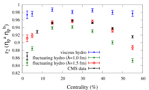
Fig. 1: Centrality dependence of factorisation ratio $r_{2}(\eta^{a}_{p},\eta^{b}_{p})$. Rapidity regions are $2.0<\eta^{a}_{p}<2.5$ and $3.0<\eta^{b}_{p}<4.0$. Results for viscous hydrodynamics (filled diamond), fluctuating hydrodynamics with $\lambda=1.0$ fm (filled circle), fluctuating hydrodynamics with $\lambda=1.5$ fm (open circle) and CMS data (filled square) [5] are shown.

Figure 1 shows results of centrality dependence of the factorisation ratio $r_{2}(\eta^{a}_{p},\eta^{b}_{p})$ compared with the CMS data [5]. Results from fluctuating hydrodynamics are always smaller than viscous hydrodynamics. In central collisions (0–10% centrality), fluctuating hydrodynamics with $\lambda=1.0$ fm is close to experimental data. On the other hand, in the mid-central collisions (10–40% centrality) fluctuating hydrodynamics with $\lambda=1.5$ fm is close to CMS data. In comparison with the result from viscous hydrodynamics, hydrodynamic fluctuations tend to break factorisation. If we choose the proper value for $\lambda$ at each centrality, we could reproduce factorisation ratios from the experimental data.

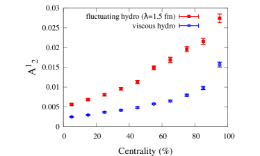
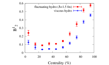
Fig. 2: Centrality dependence of the first-order Legendre coefficient $A^{1}_{2}$ and $B^{1}_{2}$ for $v_{2}$ (left figure) and $\Psi_{2}$ (right figure), respectively. Results for viscous hydrodynamics (filled diamond) and fluctuating hydrodynamics with $\lambda=1.5$ fm (filled square) are shown.

To further understand the rapidity decorrelation more comprehensively, we calculate the Legendre coefficients for rapidity dependence of anisotropic flow. For each centrality, we calculate their root mean squares,

$$A_{n}^{k} =\sqrt{\frac{1}{N_{\mathrm{ev}}}\sum^{N_{\mathrm{ev}}}_{k=1}(a_{n}^{k})^{2}}, B_{n}^{k} =\sqrt{\frac{1}{N_{\mathrm{ev}}}\sum^{N_{\mathrm{ev}}}_{k=1}(b_{n}^{k})^{2}}.$$ (7)

Here $N_{\mathrm{ev}}$ is the the number of hydrodynamic events in that centrality. Figure 2 shows results of the first-order Legendre coefficients for $v_{2}$ and $\Psi_{2}$ as a function of centrality. Results in fluctuating hydrodynamics are always larger than the ones in viscous hydrodynamics. This means hydrodynamic fluctuations give larger rapidity dependence of the magnitude of anisotropic flow coefficients and the event plane angle.

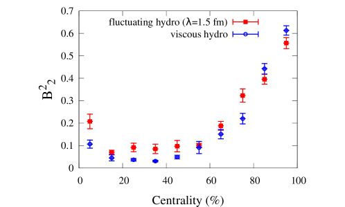
Fig. 3: Centrality dependence of second-order Legendre coefficient for event plane angle $\Psi_{2}$ ($B^{2}_{2}$). Results for viscous hydrodynamics (filled diamond) and fluctuating hydrodynamics with $\lambda=1.5$ fm (filled square) are shown.

We also analyse the second-order Legendre coefficients for the event plane angle and results are shown in Fig. 3. We call this $B^{2}_{2}$ “second-order twist” of the event plane. The second-order twist shows that the event plane angle decreases and increases again along rapidity. From the result of $B^{2}_{2}$, the second-order twist is finite and large, in particular, in central and peripheral collisions. Also it tends to be larger in fluctuating hydrodynamics than in viscous hydrodynamics. The twist behavior of the event plane angle is often discussed through the first-order coefficient. However, higher-order twists are also important in understanding event plane decorrelations.

4 Conclusion and discussions

We analysed effects of hydrodynamic fluctuations by performing numerical simulations of an integrated dynamical model based on full three dimensional fluctuating hydrodynamics. We discussed the importance of hydrodynamic fluctuations by comparing the factorisation ratios with experimental results. The fluctuating hydrodynamic model tends to break factorisation, and the factorisation ratios become closer to experimental results. Therefore hydrodynamic fluctuations play an crutial role in understanding the factorisation ratios $r_{n}(\eta^{a}_{p},\eta^{b}_{p})$.

We then proposed the Legendre coefficients $A^{k}_{2}$ and $B^{k}_{2}$ to understand the effects of hydrodynamic fluctuations. By analysing the Legendre coefficients using the fluctuating hydrodynamic model, we found hydrodynamic fluctuations tend to increase rapidity dependence. In this analysis, we found the second-order twist is large in central and peripheral collisions. Therefore higher-order twists are also important in understanding event plane decorrelations.

References

- [1] T. Hirano et al., Prog. Part. Nucl. Phys. 70 (2013) 108.
- [2] K. Murase, “Causal hydrodynamic fluctuations and their effects on high-energy nuclear collisions”, Ph.D. thesis, the University of Tokyo (2015), http://hdl.handle.net/2261/00072981.
- [3] K. Murase and T. Hirano, Nucl. Phys. A 956 (2016) 276.
- [4] T. Hirano et al., Phys. Lett. B 636 (2006) 299.
- [5] V. Khachatryan et al., (CMS Collaboration), Phys. Rev. C 92 (2015) 034911.
- [6] P. Huovinen and P. Petreczky, Nucl. Phys. A 837 (2010) 26-53.
- [7] F. Cooper and G. Frye, Phys. Fev. D 10 (1974) 186.
- [8] Y. Nara, N. Otuka, A. Ohnishi, K. Niita and S. Chiba, Phys. Rev. C 61 (2000) 024901.