Axion Cosmology with Early Matter Domination

Abstract

The default assumption of early universe cosmology is that the postinflationary universe was radiation dominated until it was about 47000 years old. Direct evidence for the radiation dominated epoch extends back until nucleosynthesis, which began during the first second. However there are theoretical reasons to prefer a period of earlier matter domination, prior to nucleosynthesis, e.g. due to late decaying massive particles needed to explain baryogenesis. Axion cosmology is quantitatively affected by an early period of matter domination, with a different axion mass range preferred and greater inhomogeneity produced on small scales. In this work we show that such increased inhomogeneity can lead to the formation of axion miniclusters in axion parameter ranges that are different from those usually assumed. If the reheating temperature is below $58$ MeV, axion miniclusters can form even if the axion field is present during inflation and has been previously homogenized. The upper bound on the typical initial axion minicluster mass is raised from $10^{-10}M_{\odot}$ to $10^{-7}M_{\odot}$, where $M_{\odot}$ is a solar mass. These results may have consequences for indirect detection of axion miniclusters, and could conceivably probe the thermal history of the universe before nucleosynthesis.

I Introduction

The QCD axion, which was invented to solve the strong CP problemPeccei and Quinn (1977); Peccei (2008), is a well-motivated candidate for dark matter. The axion mass and couplings are determined by a single parameter, the axion decay constant $f_{a}$. Laboratory, astrophysical and cosmological bounds on $f_{a}$ place it well above the weak scale. As the axion mass and couplings are inversely proportional to $f_{a}$, the axion must be extremely light, long lived, and weakly coupled.

If the axion exists, the misalignment mechanism produces axion dark matter, with an abundance that increases with $f_{a}$. It is often stated that there is an upper bound on $f_{a}$ of $10^{12}$ GeV so as to not overproduce axions. This bound may be relaxed, e.g., if the axion exists during inflation and our patch of the universe happens to have a small misalignment, or with a new depletion mechanismAgrawal et al. (2018). Without such tuning or depletion, the allowed value of $f_{a}$ is in the window $10^{9}\text{GeV}<f_{a}<10^{12}\text{GeV}$Andriamonje et al. (2007); Ayala et al. (2014); Raffelt (2008); Preskill et al. (1983); Abbott and Sikivie (1983); Dine and Fischler (1983); Vysotsky et al. (1978); Visinelli and Gondolo (2009). It has been argued that string theory favors a higher value of $f_{a}$ Banks et al. (2003); Svrcek and Witten (2006); Conlon (2006) and lighter axion than this window allows.

We can detect axions directly through the couplings with SM particles, especially the axion-photon coupling (For some reviews, see Graham et al. (2015); Bradley et al. (2003)). However, there are other interesting strategies for axion indirect detection. The axion can form gravitational bound states on small scales at very early times. If the axion is produced after inflation, then the axion field has an alignment angle which varies over a scale on the order of the Hubble horizon size of the universe at the time of formationKibble (1976). Such inhomogeneities can grow and become gravitational bound states called axion miniclusters Tkachev (1986); Hogan and Rees (1988); Sakharov and Khlopov (1994); Khlopov et al. (1998). Axion miniclusters could grow to bigger structures or boson starsKolb and Tkachev (1993); Seidel and Suen (1994), which could be detected by gravitational microlensingFairbairn et al. (2017, 2018). On the other hand, if the axion exists during inflation it is much more homogenous initiallyKolb and Tkachev (1994); Hogan and Rees (1988); Kolb and Tkachev (1996); Chang et al. (1999); Hardy (2017). For some references on possible consequences and observations connected with axion miniclusters and axion stars see refs. Barranco et al. (2013); Berezinsky et al. (2014); Tkachev (2015); Tinyakov et al. (2016); Marsh (2016); Braaten et al. (2017); Levkov et al. (2017); Bai et al. (2016); Davidson and Schwetz (2016); Visinelli et al. (2018); Enander et al. (2017); Bai and Hamada (2018); Iwazaki (2017); Eby et al. (2017); Hertzberg and Schiappacasse (2018), and for work on their structure and stability see refs Seidel and Suen (1994); Barranco and Bernal (2011); Braaten et al. (2016a); Mukaida et al. (2017); Chavanis (2016); Eby et al. (2016); Helfer et al. (2017); Jackson Kimball et al. (2018); Bai and Hamada (2018); Michel and Moss (2018). For work on the possible unique signatures of axion structure formation due to their quantum mechanical properties as light degenerate bosons see refs. Nambu and Sasaki (1990); Sikivie and Yang (2009); Rindler-Daller and Shapiro (2010, 2012); Rindler-Daller et al. (2012); Saikawa and Yamaguchi (2013); Noumi et al. (2014); Davidson and Elmer (2013); Davidson (2015); Guth et al. (2015).

The properties of axion miniclusters sensitively depend on the thermal history at the critical time when the axion starts to oscillate. For a radiation dominated universe, the corresponding temperature is typically about 1—10 GeV. This critical time is before big bang nucleosynthesis (BBN) and before the time when the big bang neutrinos decouple, and is during a time which is not connected to any established cosmological observable. If we consider a different thermal history for the universe prior to a temperature of a few MeV, we will see that the upper bound on $f_{a}$ is relaxed, and there is a significant difference in the formation history of axion miniclusters. With early matter domination, axion miniclusters can form even if the axion field has been homogenized by inflation, due to the more rapid growth of small scale primordial perturbations of the axion. Such early growth of substructure during early matter domination has been considered for other candidate dark matter particlesErickcek and Sigurdson (2011). The axion is special among dark matter candidates because its free streaming effects are almost negligible, so very small structures can form and survive.

In this paper we will consider the early cosmology of the standard invisible QCD axion with a nonstandard thermal history, with a period of early matter domination prior to nucleosynthesis. Such matter domination can be due to a heavy, weakly coupled particle whose decays reheat the universe, as is required in some theories of low scale baryogenesis. We will briefly review the theory of the axion and its corresponding cosmology, including the axion relic density and the formation of axion miniclusters in section II. In section III we will show how the axion window is opened by early matter domination. In section IV, a different story of axion minicluster formation with early matter domination is discussed. We will find that early matter domination potentially gives a larger initial characteristic mass of axion miniclusters.

II Axion Cosmology

Here we review the axion and its cosmology. (For more details about axion cosmology, seeSikivie (2008); Marsh (2016); Arvanitaki et al. (2010); Grilli di Cortona et al. (2016); Visinelli (2017).) The axion is a pseudo Nambu-Goldstone Boson resulting from the spontaneous breaking of an approximate symmetry known as the Peccei-Quinn (PQ) symmetry, due to the vacuum expectation value of a complex field known as the PQ field. We consider the following Lagrangian for the PQ field, which we call $\phi$:

$$\mathcal{L}_{\phi}=\frac{1}{2}\partial_{\mu}{\phi}^{\dagger}\partial^{\mu}\phi-\frac{\lambda}{4}(\phi^{\dagger}\phi-f_{a}^{2})^{2}+....$$ (1)

where the dots represent possible interaction terms with other particles and $f_{a}$ represents the vacuum expectation value of $\phi(x)$. The symmetry breaking will occur at a temperature $T_{\text{PQ}}$ which is roughly at the scale $f_{a}$. Classically, because of the PQ symmetry, the phase of $\phi$ is undetermined by the potential. After the PQ symmetry breaking, the phase of the PQ field receives a small potential from nonperturbative QCD effects which is minimized at a value for which the strong CP violation vanishes. Fluctuations of the phase about the minimum are parameterized by the axion field $a(x)$. Ignoring the energetically costly fluctations of the radial direction of $\phi$, we may write

$$\langle\phi(x)\rangle=f_{a}e^{ia(x)/f_{a}}.$$ (2)

When the PQ transition occurs, the potential energy with different values of $a$ is nearly degenerate, so $a$ is expected to take on a random initial value. The expansion of the universe will smooth out spatial variations in $a(x)$ but the average value of $a(x)$ remains random until late times. We say the field is misaligned with respect to its minimum, and the energy stored in this misalignment will eventually become the dark matter. There are two different cases for the cosmological evolution. In case 1, the reheating temperature of inflation is less than $T_{\text{PQ}}$ and the PQ symmetry is broken during inflation and never restored afterwards. In this case the axion field is smoothed during inflation and randomly obtain a spatially uniform vacuum expectation value $\alpha f_{a}$, where $\alpha$ is known as the misalignment angle. Quantum fluctuations in $a$ are small and proportional to the Hubble scale during inflation. As these fluctuations in $a(x)$ are isocurvature, and the cosmic microwave background observations place a strong limit on isocurvature fluctations, in case 1 there is a strong upper bound on the scale of inflationLinde (1985); Seckel and Turner (1985); Lyth (1990); Turner and Wilczek (1991); Lyth and Stewart (1992); Fox et al. (2004). In case 2 the reheating temperature after inflation is greater than $T_{\text{PQ}}$, and the PQ symmetry breaks after inflation. In this case the axion takes on random values uncorrelated over scales which are larger than the Hubble horizon at the time of PQ breaking. Topological axion strings and domain walls are then formed after inflation. Provided that there is no nontrivial unbroken discrete subgroup of the PQ symmetry, every domain wall ends on an axion string and the whole network of strings and domain walls will eventually disappearSikivie (1982); Chang et al. (1999); Gorghetto et al. (2018). The cosmological restriction that in case 2 the PQ symmetry must not have any exact discrete subgroup is a severe but achievable constraint on axion model building.

The evolution equation of the axion field in the early universe can be described by the equation

$$\left(\partial_{t}^{2}+3\frac{\dot{R}}{R}\partial_{t}-\frac{1}{R^{2}}\nabla_{x}^{2}\right)a(x)+V^{\prime}(a)=0$$ (3)

where $R$ is the scale factor, the components of x are the co-moving spatial coordinates of the universe, and $V(a)$ is the effective potential energy density of the axion field. This potential comes from non-perturbative QCD effects such as instantons’t Hooft (1976), which break the $U_{PQ}(1)$ symmetry to a $Z(N)$ discrete subgroupSikivie (1982). In case 2, we must have $N=1$ in order to avoid overclosure of the universe by a frustrated network of axion strings and domain walls, while in case 1 any such defects are inflated away (however, see ref. Kaplan and Nelson (2008) for a conceivably observable effect of axion strings outside our horizon). We can write the instanton potential qualitatively as:

$$V_{a}=f_{a}^{2}m_{a}^{2}(T)\left[1-\text{cos}\left(\frac{a}{f_{a}}\right)\right]$$ (4)

where $m_{a}$ is the axion mass, which is a function of temperature $T$. The cosine form comes from the dilute instanton gas approximation and is not exact. The form of the axion potential at low temperatures may be found in reference Braaten et al. (2016b). At high temperature ($T>$1 GeV), $m_{a}(T)$ can be estimated by instanton effects and by lattice QCD. While there is disagreement between different approaches these disagreements will not significantly change our results Dine et al. (2017). The axion mass is constant when $T$ is below the QCD scale and the calculation at low energies is reliable due to chiral perturbation theory. However, we cannot reliably predict the axion mass when $T$ is between 0.2 GeV and 1 GeV. In standard thermal history, this uncertainty will not affect our prediction of the axion relic density because the temperature at the critical time is higher than 1 GeV. However, we will see in the next section that early matter domination will decrease the critical temperature. We will assume the axion mass to be a continuous function of $T$, whose exact form will not change our main results. The full expression we will use for the axion mass follows ref. Hertzberg et al. (2008):

$$m_{a}(T)=\begin{cases}m_{a}(0),\quad\quad\quad\quad\quad\quad\quad\quad T<0.2\ \text{GeV}\\ m_{a}(0)(\frac{0.2\ \text{GeV}}{T})^{6.5},\quad 0.2\ \text{GeV}\leq T\leq 1\ \text{GeV}\\ bm_{a}(0)(\frac{0.2\ \text{GeV}}{T})^{4},\quad\quad\quad\quad T>1\ \text{GeV}\ ,\end{cases}$$ (5)

where $b=0.018$ and $m_{a}(0)=(78\ \text{MeV})^{2}/f_{a}$, and $m_{a}(0)$ is the axion mass at zero-temperature. Given the thermal history of early universe, the axion mass is determined by cosmic time. The first three terms in Eq.(3) are proportional to $t^{-2}$, which are the dominant terms until late times. We define the critical time $t_{1}$ at which the potential term becomes important relative to the Hubble expansion term to be:

$$H(t_{1})=m_{a}(T(t_{1}))$$ (6)

The mean value of the axion field does not evolve much before the time $t_{1}$. After $t_{1}$ the axion field begins to oscillate and its energy density behaves approximately like nonrelativistic matter. The energy density of a uniform oscillating axion field may be interpreted as the energy density of axion particles at rest. The number of axion particles per co-moving volume is adiabatically conserved because the axion mass changes slowly compared with the oscillation period. In case 1, where axions were homogenized by inflation, axions at rest are the dominate initial component of axions in the universe. In case 2, some spatial variation in the axion field remains which is interpreted as axions with non zero momentum, and also a substantial number of axions are produced via the decay of axion strings and domain walls. The number density of axions at rest isPreskill et al. (1983); Abbott and Sikivie (1983); Dine and Fischler (1983):

$$n_{a}^{vac,0}(t)=\frac{1}{2}m_{a}(t)f_{a}^{2}\alpha^{2}\ .$$ (7)

In case 1, $\alpha$ is uniform throughout our universe and its random value introduces uncertainties in our prediction. We simply treat it as a $O(1)$ constant and do not consider the possible consequences of a small misalignment angle. In case 2, $\alpha$ is randomly distributed taking on many different values throughout our observable universe, and is roughly uniform on scales on the order of the Hubble horizon size at the time of PQ symmetry breaking. As there are many such volumes contained within our current horizon we may average over the different initial values. The dominant source of theory uncertainty for the axion density in case 2 is from the computation of the number of axions produced from the decay of axion strings and domain walls.

II.1 Axion Relic Density

In case 1, we can directly get the current energy density of the axion:

$$\rho_{a}^{\text{vac},0}=\frac{1}{2}m_{a}(0)m_{a}(t_{1})f_{a}^{2}\alpha^{2}\left(\frac{R_{1}}{R}\right)^{3}$$ (8)

where $t_{1}$ is the critical time when axion starts to oscillate and $R_{1}/R$ is the ratio of the scale factor at the critical time to that at present. The number of axions is approximately conserved and the energy density is simply the number density multiplied by $m_{a}(0)$. Combined with a radiation dominated thermal history, we obtain the following energy density in case 1:

$$\Omega_{a}\sim 0.15\>\left(\frac{f_{a}}{10^{12}\text{GeV}}\right)^{7/6}\left(\frac{0.7}{h}\right)^{2}\alpha^{2}$$ (9)

where $h$ is defined to give the Hubble constant $H_{0}=\text{100km/s}\cdot h\cdot\text{Mpc}$.

Case 2 is more complicated because axion strings and domain walls will decay to axions and give an extra contribution to the axion relic density. There is a potential so-called domain wall problem when the PQ symmetry group $U_{PQ}(1)$ has non trivial discrete $Z(N)$ subgroup, as in this case there is an N fold degeneracy of the vacuumSikivie (1982). We assume in case 2 that $N=1$ for viable axion cosmology Vilenkin and Everett (1982); Lazarides and Shafi (1982). In this case the domain walls are unstable and bounded by strings. The string decay contribution to the axion relic density Gorghetto et al. (2018) is highly uncertain and we simply parameterize the uncertainty. Following ref. Hagmann and Sikivie (1991) we write:

$$\rho_{a}^{\text{str}}=m_{a}(0)n_{a}^{\text{str}}(t_{1})\left(\frac{R_{1}}{R_{0}}\right)^{3}\backsimeq Ym_{a}(0)\frac{f_{a}^{2}}{m_{a}(t_{1})}\left(\frac{R_{1}}{R_{0}}\right)^{3}$$ (10)

where $m_{a}(0)$ is the axion mass at zero temperature, $m_{a}(t_{1})$ is the axion mass at the critical time when axion starts to oscillate, and $Y$ is an order one factor which is determined by details such as the efficiency of string decay, the axion string number per horizon and average energy of the axions emitted in a string decay. We simply assume a value for $Y$ here and study what will be different in a nonstandard thermal history.

The last step is to estimate the contribution from higher momentum modes. Assume that axion field varies by $f_{a}$ from one horizon to the next, we can obtain the number density distribution of higher momentum modes of the axion:

$$\frac{n_{a}}{d\omega}\sim\frac{f_{a}^{2}}{2t^{2}\omega^{2}}$$ (11)

Only frequencies which enter the horizon are physically relevant for this work. Integrating over $\omega>1/H(t_{1})$ in Eq.(11) gives us the contribution from vacuum realignment of higher momentum modes:

$$\rho_{a}^{\text{vac},1}\sim\frac{m_{a}(0)f_{a}^{2}}{2m_{a}(t_{1})}\left(\frac{R_{1}}{R_{0}}\right)^{3}$$ (12)

So the contribution from higher momentum modes is roughly the same as that of the zero momentum mode. Including an estimate of the contribution from higher momentum modes and string decays, the relic density could be written as:

$$\Omega_{a}\sim 0.6\>\left(\frac{f_{a}}{10^{12}\text{GeV}}\right)^{7/6}\left(\frac{0.7}{h}\right)^{2}$$ (13)

Notice that the axion relic density in case 2 is generally greater than in case 1 for a given $f_{a}$.

From Eqs.(9),(13), we see an upper bound for $f_{a}$ in order to avoid overproduction of axion dark matter. The upper bounds for case 1 and case 2 with standard thermal history are respectively $\sim 1.4\times 10^{12}$ GeV and $\sim 4.4\times 10^{11}$ GeV, with order one uncertainties in both cases. Combined with other constraints, we obtain the so-called axion window, $10^{9}\ \text{GeV}<f_{a}<10^{12}\ \text{GeV}$.

II.2 Axion Miniclusters

In case 2, where inflation happens before the PQ phase transition, the initial misalignment angle will not be homogenized by inflation. Therefore, its value will vary randomly from one horizon to another. An inhomogeneity with $\delta\rho_{a}/\rho_{a}=\mathcal{O}(1)$ is produced when the axion mass turns on. If not erased by the free-streaming effect, gravitationally bound objects , which are called axion miniclusters, may form at the time $t_{eq}$ when energy density of radiation and matter are equalHogan and Rees (1988); Kolb and Tkachev (1993, 1996); Chang et al. (1999).

Because axions are typically very cold, free-streaming effects will not restrain the form of axion miniclustersKolb and Tkachev (1996); Chang et al. (1999). In case 1, only zero mode axions due to vacuum misalignment are produced and there is no velocity dispersion. In case 2, there are higher momentum modes produced by vacuum realignment axions produced by wall decay and string decay. They will give us some non-zero velocity dispersion but it can still be shown that free-streaming will not homogenize the axions.

The characteristic minicluster mass is given by the total mass of axions contained within the horizon at the critical time when the axion starts to oscillate:

$$M_{mc}=\frac{1}{2}m_{a}(0)m_{a}(t_{1})f_{a}^{2}\>\frac{4\pi}{3}\left(\frac{1}{H(t_{1})}\right)^{3}$$ (14)

Since the number of axions per co-moving volume is conserved, we must take the evolution of the axion mass into consideration in computing the mass of axion miniclusters. If we assume a standard thermal history where the early universe is dominated by radiation, the corresponding temperature of the critical time is:

$$T_{1}\simeq 1\>\text{GeV}\left(\frac{10^{12}\text{GeV}}{f_{a}}\right)^{1/6}$$ (15)

Thus we obtain the mass of axion miniclusters in a standard thermal history:

$$M_{mc}=3.7\times 10^{-10}M_{\odot}\left(\frac{f_{a}}{10^{12}\text{GeV}}\right)^{5/3}$$ (16)

where $M_{\odot}$ is the solar mass. Note that there are various strategies to estimate the mass of axion miniclusters, such as calculating the axions contained within the horizon at $t_{eq}$. A detailed study requires the calculation of the mass function of axion minicluster through its power spectrum. The evolution of axion miniclusters in the nonlinear region should be also included, which allows for the possibility of larger axion stars. Such evolution is outside the scope of this paper. Our main goal is to find what will be changed during a nonstandard thermal history. Therefore, we focus on the linear region and give the estimate of the change in the initial axion minicluster mass with early matter domination.

III Opening the Axion Window

Nothing so far has been directly detected from the epoch after inflation and before nucleosynthesis. The “standard” assumption about that period is that the inflationary energy density decayed to a hot thermal relativistic plasma containing all the particles in the standard model and possibly some extensionAlbrecht et al. (1982); Turner (1983); Traschen and Brandenberger (1990); Kofman et al. (1994), reheating the universe, and the universe remained radiation dominated until the temperature dropped below about 1 eV. However, the inflationary energy density could also decay to some nonstandard massive particles, which could be long lived and come to dominate the energy of the universe, as the energy density of nonrelativistic particles evolves with the scale factor $R$ as $R^{-3}$ while that of radiation evolves as $R^{-4}$. The success of standard nucleosynthesis implies that any such massive long lived particles have decayed and brought the universe to radiation domination before a temperature of order a few MeV. A pre-nucleosynthesis epoch with energy dominated by nonrelativistic massive particles is called an Early Matter Dominated Epoch (EMDE). Such a scenario is favored by some baryogenesis models as a way to satisfy the out of equilibrium Sakharov condition for producing the asymmetry between matter and anti-matter. One top down motivated example of an EDME is motivated by stabilized moduli in string theory de Carlos et al. (1993); Banks et al. (1994); Acharya et al. (2014). Another motivation is to produce curvature perturbations in the curvaton modelMollerach (1990); Linde and Mukhanov (1997); Lyth and Wands (2002); Moroi and Takahashi (2001). There are other cosmological consequences of a EDME scenario, such as boosting the thermal dark matter annihilation rateKhlopov and Polnarev (1982); Erickcek et al. (2016); Erickcek (2015); Choi and Takahashi (2017).

An EDME will affect the axion relic density and expand the allowed range of $f_{a}$. The co-moving entropy density will increase during the decay of the massive particles, which will decrease the ratio of axions to photons Giudice et al. (2001); Grin et al. (2008); Visinelli and Gondolo (2010); Kane et al. (2015); Lazarides et al. (1990). We may calculate the abundance of relic axions with an EDME by solving Boltzmann equations. We will use the example of matter domination by a particle $\Phi$, whose spin is irrelevant. In the three-fluid model for reheating, the evolution of energy density is give by:

$$\begin{split}&\frac{d\rho_{\Phi}}{dt}+3H\rho_{\Phi}=-\Gamma_{\phi}\rho_{\Phi}\\ &\frac{d\rho_{r}}{dt}+4H\rho_{\Phi}=\Gamma_{\phi}\rho_{\Phi}\end{split}$$ (17)

where $\rho_{\Phi}$ is the energy density of $\Phi$, $\rho_{r}$ is the energy density of radiation, $\Gamma_{\Phi}$ is the decay rate of the massive particle and $H$ is the Hubble parameter. We have neglected the contribution from the axion field because it contributes only a minor energy density to the early universe. Combined with the Friedmann equations we can solve the exact energy density of the massive particle and radiation as a function of cosmic time. We assume that the radiation plasma reaches its equilibrium state instantaneously after $\Phi$ decays. This is reasonable since the decay rate is relatively slow compared with the thermalization rate of the light particles. In this way we can also obtain the temperature in terms of cosmic time, which also gives us the mass of the axion as a function of time. Once we know the axion mass as a function of time, the critical time $t_{1}$ when the axion starts to oscillate can be estimated from $H(t_{1})=m_{a}(t_{1})$. We then use the adiabatic approximation with the co-moving number density of axions conserved after the critical time, which gives the evolution of axion number density at time $t>t_{1}$:

$$n_{a}(t)=\frac{1}{2}m_{a}(t_{1})f_{a}^{2}\left(\frac{R(t_{1})}{R(t)}\right)^{3}\ .$$ (18)

When the universe is dominated again by radiation, the entropy density behaves exactly like $R^{-3}$ and $n_{a}/s$ is conserved. The entropy of universe is dominated by radiation. We can thus obtain the current axion density. The axion energy density must be less than the dark matter relic density. We can therefore obtain an upper bound on the axion decay constant $f_{a}$ as a function of the reheat temperature $T_{rh}$. The reheat temperature is directly determined by the decay rate of oscillating scalar field.

$$\frac{\pi^{2}}{30}g_{*}(T_{rh})T_{rh}^{4}=\frac{3E_{pl}^{2}\Gamma_{\phi}^{2}}{8}$$ (19)

where $g_{*}$ is the effective number of degrees of freedom, and $E_{pl}$ is the planck energy.

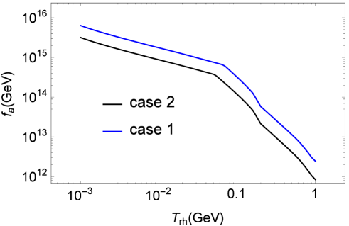
Figure 1: New upper bound on the axion decay constant under early matter domination with reheating temperature $T_{rh}$, assuming the various undetermined constants are of order 1. The blue curve is for case 1 and black curve is for case 2.

The upper bound on $f_{a}$ does not depend on the EDME unless the reheat temperature is below the temperature at the critical time when the axion field begins to oscillate. Thus, only a reheat temperature greater than about 1 MeV (So it happens before nucleosynthesis) and less than about 1 GeV is relevant for a new story of axion cosmology.

IV Axion Miniclusters with Early Matter Domination

Since the axion window is widened by early matter domination, it is straightforward to show that the possible mass of axion miniclusters increases with a greater axion decay constant. A nontrivial result is that the formation of axion miniclusters is even allowed in case 1, which is not expected with a standard thermal history. The formation of miniclusters results because matter density perturbations will grow linearly with the scale factor during the EMDE while they only grow logarithmically during radiation domination. Generally an EDME allows for an increase in small scale dark matter structure formationErickcek and Sigurdson (2011); Fan et al. (2014). But axion miniclusters are especially sensitive to such a period because axions are extremely cold. Free streaming effects are negligible for axions which allows for tiny structures.

For miniclusters in case 2, the correction to the axion minicluster mass from early matter domination is straightforward. We simply estimate the critical time with early matter domination and use the same formula Eq.(14). However, in case 1 with standard thermal history axion miniclusters do not generally form. In contrast, the primordial perturbations of axion field that enter the horizon during the EDME can grow linearly, and form an axion minicluster. If such structures form during the EDME then they are dominated by the massive particles which will decay to reheat the universe, and when those particles decay the structures will be erased. But structures that form during and after the radiation dominated epoch persist. We estimate the initial size of such structures as follows. We assume a nearly scale invariant primordial perturbation of about $10^{-4}$Komatsu et al. (2011). Axions are frozen before the critical time at which axion oscillations begin. When there is a period of EDME and the reheating time is later than the critical time, initial inhomogeneities which are inside the horizon will grow linearly with the scale factor. We therefore find the scale at which perturbations of a given scale size enter the horizon during the EDME, and grow to $\delta\rho/\rho$ of order 1 at the end of the early matter domination epoch. Continued logarithmic growth of these structures will allow for axion minicluster formation at the end of radiation domination. Only specific combinations of $f_{a}$ and $T_{rh}$ will allow the formation of axion miniclusters in case 1. In general larger axion decay constants lead to a later critical time at which the axion starts to oscillate, and these structures grow linearly with the scale factor only during the EDME. In case 1, formation of axion miniclusters implies a reheating temperature dependent upper bound on $f_{a}$.

IV.1 Cosmological Perturbations

In order to obtain the axion minicluster mass in case 1, we need to find the perturbation growth during early matter domination. Generally the perturbations will grow linearly with the scale factor if the universe is dominated by matter. In principle the situation is more complicated for the axion because its mass is also changing with time, however the term from the changing mass is negligible compared with the linear growth term for the following reasons: 1. The temperature is typically less than 1 GeV at the critical time when the axion perturbation starts to grow. The axion mass will not change much at that time. 2. The axion mass is temperature dependent and gives perturbations proportional to $\dot{T}/T$, which is actually a logarithmic growth term. We can treat the oscillating scalar field, the radiation and cold axions as perfect fluids with energy momentum tensorsKodama and Sasaki (1984); Malik et al. (2003); Lemoine and Martin (2007):

$$T^{\mu\nu}=(\rho+p)u^{\mu}u^{\nu}+pg^{\mu\nu}$$ (20)

Where $u^{\mu}\equiv dx^{\mu}/d\lambda$ is the four-velocity. For cold axions and $\Phi$ particles, the pressure is zero and for radiation $p=\rho/3$. Due to the decay of $\Phi$ particles, different fluids exchange energy covariantly:

$$\nabla(^{(i)}T^{\mu}_{\nu})=Q^{(i)}_{\nu}$$ (21)

Where $i$ denotes different fluids. For the energy exchange vector:

$$\begin{split}&Q^{\phi}_{\nu}={}^{(\phi)}T_{\mu\nu}u^{\mu}_{\phi}\Gamma_{\phi}\\ &Q^{r}_{\nu}=-Q^{\phi}_{\nu}-Q^{a}_{\nu}\\ &Q^{a}_{\nu}=-{}^{(a)}T_{\mu\nu}u^{\mu}_{a}\frac{\dot{m}_{a}}{m_{a}}\end{split}$$ (22)

During the early matter domination, $Q^{a}\ll Q^{\phi}$. So the the perturbation in axions should not change the evolution of the radiation perturbation. To obtain the perturbation equations, we start with the perturbed metric

$$\text{d}s^{2}=-(1+2\Psi)\text{d}t^{2}+a^{2}(t)\delta_{ij}(1-2\Psi)dx^{i}dx^{j}$$ (23)

Thus we have the perturbation of the four-velocity:

$$\begin{split}&u^{0}=1-\Psi\\ &u^{j}_{i}=(1-\Psi)V_{(i)}^{j}\end{split}$$ (24)

where $V_{(i)}^{j}\equiv\text{d}x^{j}/\text{d}t$ is the fluid velocity of the $i$th fluid. With the perturbation of energy density of each fluid $\rho_{i}=\rho^{0}_{i}(1+\delta_{i})$, we can write the dominant term and the first order perturbation term of $Q$

$$\begin{split}&Q^{(\phi)}_{0}=\Gamma_{\phi}\rho^{0}_{\phi}(1+\delta_{\phi}+\Psi)\\ &Q^{(\phi)}_{j}=-\Gamma_{\phi}\rho^{0}_{\phi}a^{2}\delta_{kj}V^{k}_{\phi}\\ &Q^{(a)}_{0}=-\frac{\dot{m}_{a}}{m_{a}}\rho^{0}_{a}(1+\delta_{a}+\Psi)\\ &Q^{(a)}_{j}=\frac{\dot{m}_{a}}{m_{a}}\rho^{0}_{a}a^{2}\delta_{kj}V^{k}_{a}\end{split}$$ (25)

$\Gamma_{\phi}$ and $\frac{\dot{m}_{a}}{m_{a}}$ are significantly different. One is a constant and the other has perturbation determined by the temperature perturbation of the radiation. Compared with the Hubble parameter, $\Gamma_{\phi}$ is usually negligible but $\frac{\dot{m}_{a}}{m_{a}}$ may be important for the perturbation function.

Expressing $Q_{\nu}$ with in terms of the zero-order and first-order perturbations, we can combine equation (1) and (2) to get simple results that determine the perturbation:

$$\begin{split}&\frac{\text{d}{\delta}}{\text{d}t}+(1+w)\frac{\theta}{a}+3(1+w)\frac{\text{d}\Psi}{\text{d}t}=\frac{1}{\rho^{0}}[Q_{0}^{(0)}\delta-Q_{0}^{(1)}]\ ,\\ &\frac{\text{d}\theta}{\text{d}t}+(1-3w)H\theta+\frac{\nabla^{2}\Psi}{a}+\frac{w}{1+w}\frac{\nabla^{2}\delta}{a}\\ &=\frac{1}{\rho_{0}}\left[\frac{\partial_{i}Q_{i}}{a(1+w)}+Q_{0}^{(0)}\theta\right]\ ,\end{split}$$ (26)

where $w=p/\rho$ is the fluid’s equation of state parameter, and $\theta=a\partial_{i}V^{i}$ is the divergence of fluid’s conformal velocity. $Q_{0}^{(0)}$ and $Q_{0}^{(1)}$ are respectively the zero-order and first-order components of $Q$.

It can be generally shown that the metric perturbation is frozen in a matter-dominated universe. We define the beginning of early matter domination as $a=1$ and its corresponding Hubble parameter is $H_{0}$. For convenience, we also define dimensionless parameter $\widetilde{\theta_{\phi}}\equiv\theta_{\phi}/H_{0}$, $\widetilde{k}\equiv k/H_{0}$. Therefore we can represent our equations during early matter domination in the following way:

$$\begin{split}&a^{-1/2}\delta^{{}^{\prime}}_{\phi}(a)+\widetilde{\theta}_{\phi}(a)=0\ ,\\ &a^{1/2}\widetilde{\theta}_{\phi}^{{}^{\prime}}(a)+a^{-1/2}\widetilde{\theta}_{\phi}(a)+\widetilde{k}^{2}\Psi=0\ ,\\ &a^{1/2}\widetilde{\theta}^{{}^{\prime}}_{a}(a)+a^{-1/2}\widetilde{\theta}_{a}(a)+\widetilde{k}^{2}\Psi=0\ ,\\ &a^{-1/2}\delta^{{}^{\prime}}_{a}(a)+\widetilde{\theta}_{a}(a)=\frac{a\dot{m}_{a}}{m_{a}H(t_{1})}\Psi\ ,\\ \end{split}$$ (27)

where a prime represents the derivative to scale factor, and $H(t_{1})$ is the Hubble parameter at the critical time. It is not hard to show that the term $\frac{a\dot{m}_{a}}{m_{a}H(t_{1})}$ only causes a logarithmic growth, which could be neglected compared with the linear growth. Eventually the perturbation for modes that have already entered horizon before the critical time is:

$$\delta_{a}(a,k)=2\Psi_{0}+\frac{2k^{2}}{3H(t_{1})^{2}}a\Psi_{0}$$ (28)

where $\Psi_{0}$ represents the primordial perturbation of quantum fluctuation during inflation, which is about $10^{-4}$. Now it is clear that perturbations grow linearly with scale factor $a$ during early matter dominated epoch. To form axion miniclusters efficiently at the end of radiation domination, $\delta_{a}$ must be grow up to about 1. Actually the formation of axion minicluster is complicated here because the growth depends on momentum. We can actually obtain the transfer function for axion generally and calculate the mass function of axion minicluster with Press-Schechter formalism. However, axion perturbation grows to the nonlinear region very early and it is hard to predict its later evolution. In this paper we just estimate the original axion minicluster mass and leave its evolution for future research.

IV.2 Formation of Axion Miniclusters

A perturbation $\delta_{a}(a,k)$ will start to grow when $k$ enters the horizon. The momentum modes which have already entered the horizon at the critical time ($k>H(t_{1})$) will grow the largest. Typically large $k$ represents smaller axion miniclusters so we only care about $k<H(t_{1})$. Therefore the criterion for axion miniclusters formation in case 1 is if $\delta_{a}(a_{e},H(t_{1}))$ is larger than 1, where $a_{e}$ is the scale factor at the end of early matter domination. It can be drawn together with the upper bound for allowed axion density (See FIG.(2)). Parameters must be below the bound from axion density to not overproduce axions. To form axion miniclusters, the parameters must be below the orange curve. For case 1, if all the dark matter is axions, the reheating temperature must be below about 60 MeV in order to obtain axion miniclusters.

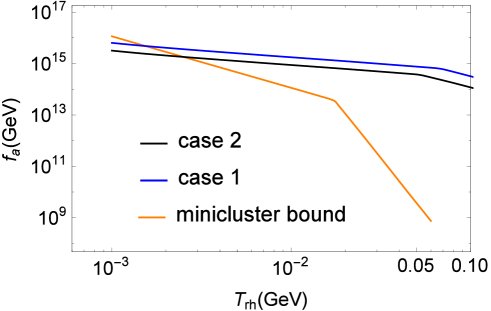
Figure 2: The blue and black curve which indicate the bound on $f_{a}$ from the relic axion density is part of FIG.(1). The orange curve represents the upper bound for axion decay constant if growth is sufficient for formation of axion miniclusters in case 1. (In case 2, due to larger initial inhomogeneity on small scales, axion miniclusters can generally form.) The axion density increases with the axion decay constant. When the reheating temperature is sufficiently low, dark matter axions can comprise all of the dark matter as well as form axion miniclusters in case 1, because the blue curve is below the orange curve.

The final step of this chapter is to determine the mass of axion miniclusters with early matter domination. In case 2 it is can be straightforwardly done by substituting the new critical time. In case 1, suppose that we have some $k_{c}<H(t_{1})$ which satisfies:

$$\delta_{a}(a_{e},k_{c})=1$$ (29)

where $a_{e}$ is the scale factor at the end of early matter domination. $k_{c}$ represents the characteristic modes that eventually grow to axion miniclusters. Suppose that $k_{c}$ enters the horizon at time $t_{c}$, $H(t_{c})=k_{c}$. The corresponding axion number density at $t_{c}$ is:

$$n_{ac}=\frac{1}{2}m_{a}(t_{1})f_{a}^{2}(\frac{R(t_{1})}{R(t_{c})})^{3}$$ (30)

where $t_{1}$ is the critical time and $R$ is the scale factor of universe. Therefore axion minicluster mass mass could be estimated by:

$$M_{mc}=\frac{4}{3}\pi m_{a}(0)(\frac{1}{k_{c}})^{3}n_{ac}$$ (31)

As an example, we calculate how axion minicluster mass changes with axion decay constant at reheating temperature $3$ MeV, as shown in FIG.(3).

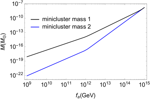
Figure 3: The black curve and the blue curve respectively represent the axion minicluster mass in case 1 and case 2 when the reheating temperature is 3 MeV.

From FIG.(3) we can see that the upper limit on the axion minicluster mass has increased to $10^{-8}M_{\odot}$, where $M_{\odot}$ is the solar mass. In comparison, from Eq.(16), with the standard thermal history the maximum minicluster mass is $\sim 8.5\times 10^{-14}M_{\odot}$. It is worth noting that the initial axion minicluster mass is typically less than the critical mass at which an axion star becomes unstable to gravitational collapseVisinelli et al. (2018); Helfer et al. (2017); Chavanis (2016); Michel and Moss (2018) so the miniclusters will not form black holes.

V Conclusions

We have shown that the axion window is wider and the formation history of axion miniclusters is significantly affected by a period of matter domination prior to nucleosynthesis. The axion can be lighter, and the maximum mass of axion miniclusters is increased. Furthermore axion miniclusters can form even in the case where the PQ symmetry breaking occurs before inflation. In this work we have estimated the characteristic mass of axion miniclusters at the time of formation. More detailed numerical study about the evolution of axion miniclusters is needed to obtain the information about axion miniclusters at present, including the mass function of axion miniclusters, the percentage of axions that form axion miniclusters, and the percentage of axion miniclusters that form boson stars or black holes. The evolution of axion miniclusters after their formation and the fraction of axions that finally become gravitationally bound objects requires detailed numerical study, which is beyond the scope of this paper. Such work would be important, as indirect detection of axion miniclusters could possibly provide evidence for both the existence of the axion and for a nonstandard thermal history of the very early universe.

VI Acknowledgements

This work was supported in part by the by the DOE under grant DE-SC0011637 and by the Kenneth K. Young Memorial Endowed Chair.

References

- Peccei and Quinn (1977) R. D. Peccei and H. R. Quinn, Phys. Rev. Lett. 38, 1440 (1977), [,328(1977)].
- Peccei (2008) R. D. Peccei, Lect. Notes Phys. 741, 3 (2008), [,3(2006)], eprint hep-ph/0607268.
- Agrawal et al. (2018) P. Agrawal, G. Marques-Tavares, and W. Xue, JHEP 03, 049 (2018), eprint 1708.05008.
- Andriamonje et al. (2007) S. Andriamonje et al. (CAST), JCAP 0704, 010 (2007), eprint hep-ex/0702006.
- Ayala et al. (2014) A. Ayala, I. Domínguez, M. Giannotti, A. Mirizzi, and O. Straniero, Phys. Rev. Lett. 113, 191302 (2014), eprint 1406.6053.
- Raffelt (2008) G. G. Raffelt, Lect. Notes Phys. 741, 51 (2008), [,51(2006)], eprint hep-ph/0611350.
- Preskill et al. (1983) J. Preskill, M. B. Wise, and F. Wilczek, Phys. Lett. B120, 127 (1983), [,URL(1982)].
- Abbott and Sikivie (1983) L. F. Abbott and P. Sikivie, Phys. Lett. B120, 133 (1983), [,URL(1982)].
- Dine and Fischler (1983) M. Dine and W. Fischler, Phys. Lett. B120, 137 (1983), [,URL(1982)].
- Vysotsky et al. (1978) M. I. Vysotsky, Ya. B. Zeldovich, M. Yu. Khlopov, and V. M. Chechetkin, Pisma Zh. Eksp. Teor. Fiz. 27, 533 (1978), [JETP Lett.27,502(1978)].
- Visinelli and Gondolo (2009) L. Visinelli and P. Gondolo, Phys. Rev. D 80, 035024 (2009), URL https://link.aps.org/doi/10.1103/PhysRevD.80.035024.
- Banks et al. (2003) T. Banks, M. Dine, P. J. Fox, and E. Gorbatov, JCAP 0306, 001 (2003), eprint hep-th/0303252.
- Svrcek and Witten (2006) P. Svrcek and E. Witten, JHEP 06, 051 (2006), eprint hep-th/0605206.
- Conlon (2006) J. P. Conlon, JHEP 05, 078 (2006), eprint hep-th/0602233.
- Graham et al. (2015) P. W. Graham, I. G. Irastorza, S. K. Lamoreaux, A. Lindner, and K. A. van Bibber, Ann. Rev. Nucl. Part. Sci. 65, 485 (2015), eprint 1602.00039.
- Bradley et al. (2003) R. Bradley, J. Clarke, D. Kinion, L. J. Rosenberg, K. van Bibber, S. Matsuki, M. Muck, and P. Sikivie, Rev. Mod. Phys. 75, 777 (2003).
- Kibble (1976) T. W. B. Kibble, J. Phys. A9, 1387 (1976).
- Tkachev (1986) I. I. Tkachev, Sov. Astron. Lett. 12, 305 (1986), [Pisma Astron. Zh.12,726(1986)].
- Hogan and Rees (1988) C. J. Hogan and M. J. Rees, Phys. Lett. B205, 228 (1988).
- Sakharov and Khlopov (1994) A. S. Sakharov and M. Yu. Khlopov, Phys. Atom. Nucl. 57, 485 (1994), [Yad. Fiz.57,514(1994)].
- Khlopov et al. (1998) M. Yu. Khlopov, A. S. Sakharov, and D. D. Sokoloff, in 2nd International Workshop on Birth of the Universe and Fundamental Physics Rome, Italy, May 19-24, 1997 (1998), eprint hep-ph/9812286.
- Kolb and Tkachev (1993) E. W. Kolb and I. I. Tkachev, Phys. Rev. Lett. 71, 3051 (1993), eprint hep-ph/9303313.
- Seidel and Suen (1994) E. Seidel and W.-M. Suen, in On recent developments in theoretical and experimental general relativity, gravitation, and relativistic field theories. Proceedings, 7th Marcel Grossmann Meeting, Stanford, USA, July 24-30, 1994. Pt. A + B (1994), pp. 1067–1069, eprint gr-qc/9412062.
- Fairbairn et al. (2017) M. Fairbairn, D. J. E. Marsh, and J. Quevillon, Phys. Rev. Lett. 119, 021101 (2017), eprint 1701.04787.
- Fairbairn et al. (2018) M. Fairbairn, D. J. E. Marsh, J. Quevillon, and S. Rozier, Phys. Rev. D97, 083502 (2018), eprint 1707.03310.
- Kolb and Tkachev (1994) E. W. Kolb and I. I. Tkachev, Phys. Rev. D49, 5040 (1994), eprint astro-ph/9311037.
- Kolb and Tkachev (1996) E. W. Kolb and I. I. Tkachev, Astrophys. J. 460, L25 (1996), eprint astro-ph/9510043.
- Chang et al. (1999) S. Chang, C. Hagmann, and P. Sikivie, Phys. Rev. D59, 023505 (1999), eprint hep-ph/9807374.
- Hardy (2017) E. Hardy, JHEP 02, 046 (2017), eprint 1609.00208.
- Barranco et al. (2013) J. Barranco, A. C. Monteverde, and D. Delepine, Phys. Rev. D87, 103011 (2013), eprint 1212.2254.
- Berezinsky et al. (2014) V. S. Berezinsky, V. I. Dokuchaev, and Y. N. Eroshenko, Phys. Usp. 57, 1 (2014), [Usp. Fiz. Nauk184,3(2014)], eprint 1405.2204.
- Tkachev (2015) I. I. Tkachev, JETP Lett. 101, 1 (2015), [Pisma Zh. Eksp. Teor. Fiz.101,no.1,3(2015)], eprint 1411.3900.
- Tinyakov et al. (2016) P. Tinyakov, I. Tkachev, and K. Zioutas, JCAP 1601, 035 (2016), eprint 1512.02884.
- Marsh (2016) D. J. E. Marsh, Phys. Rept. 643, 1 (2016), eprint 1510.07633.
- Braaten et al. (2017) E. Braaten, A. Mohapatra, and H. Zhang, Phys. Rev. D96, 031901 (2017), eprint 1609.05182.
- Levkov et al. (2017) D. G. Levkov, A. G. Panin, and I. I. Tkachev, Phys. Rev. Lett. 118, 011301 (2017), eprint 1609.03611.
- Bai et al. (2016) Y. Bai, V. Barger, and J. Berger, JHEP 12, 127 (2016), eprint 1612.00438.
- Davidson and Schwetz (2016) S. Davidson and T. Schwetz, Phys. Rev. D93, 123509 (2016), eprint 1603.04249.
- Visinelli et al. (2018) L. Visinelli, S. Baum, J. Redondo, K. Freese, and F. Wilczek, Phys. Lett. B777, 64 (2018), eprint 1710.08910.
- Enander et al. (2017) J. Enander, A. Pargner, and T. Schwetz, JCAP 1712, 038 (2017), eprint 1708.04466.
- Bai and Hamada (2018) Y. Bai and Y. Hamada, Phys. Lett. B781, 187 (2018), eprint 1709.10516.
- Iwazaki (2017) A. Iwazaki (2017), eprint 1707.04827.
- Eby et al. (2017) J. Eby, M. Leembruggen, J. Leeney, P. Suranyi, and L. C. R. Wijewardhana, JHEP 04, 099 (2017), eprint 1701.01476.
- Hertzberg and Schiappacasse (2018) M. P. Hertzberg and E. D. Schiappacasse (2018), eprint 1805.00430.
- Barranco and Bernal (2011) J. Barranco and A. Bernal, Phys. Rev. D83, 043525 (2011), eprint 1001.1769.
- Braaten et al. (2016a) E. Braaten, A. Mohapatra, and H. Zhang, Phys. Rev. Lett. 117, 121801 (2016a), eprint 1512.00108.
- Mukaida et al. (2017) K. Mukaida, M. Takimoto, and M. Yamada, JHEP 03, 122 (2017), eprint 1612.07750.
- Chavanis (2016) P.-H. Chavanis, Phys. Rev. D94, 083007 (2016), eprint 1604.05904.
- Eby et al. (2016) J. Eby, M. Leembruggen, P. Suranyi, and L. C. R. Wijewardhana, JHEP 12, 066 (2016), eprint 1608.06911.
- Helfer et al. (2017) T. Helfer, D. J. E. Marsh, K. Clough, M. Fairbairn, E. A. Lim, and R. Becerril, JCAP 1703, 055 (2017), eprint 1609.04724.
- Jackson Kimball et al. (2018) D. F. Jackson Kimball, D. Budker, J. Eby, M. Pospelov, S. Pustelny, T. Scholtes, Y. V. Stadnik, A. Weis, and A. Wickenbrock, Phys. Rev. D97, 043002 (2018), eprint 1710.04323.
- Michel and Moss (2018) F. Michel and I. G. Moss (2018), eprint 1802.10085.
- Nambu and Sasaki (1990) Y. Nambu and M. Sasaki, Phys. Rev. D42, 3918 (1990).
- Sikivie and Yang (2009) P. Sikivie and Q. Yang, Phys. Rev. Lett. 103, 111301 (2009), eprint 0901.1106.
- Rindler-Daller and Shapiro (2010) T. Rindler-Daller and P. R. Shapiro, ASP Conf. Ser. 432, 244 (2010), eprint 0912.2897.
- Rindler-Daller and Shapiro (2012) T. Rindler-Daller and P. R. Shapiro, Mon. Not. Roy. Astron. Soc. 422, 135 (2012), eprint 1106.1256.
- Rindler-Daller et al. (2012) T. Rindler-Daller, T. Rindler-Daller, P. R. Shapiro, and P. R. Shapiro, in 6th International Meeting on Gravitation and Cosmology Guadalajara, Jalisco, Mexico, May 21-25, 2012 (2012), pp. 163–182, [,163(2014)], eprint 1209.1835, URL http://inspirehep.net/record/1184893/files/arXiv:1209.1835.pdf.
- Saikawa and Yamaguchi (2013) K. Saikawa and M. Yamaguchi, Phys. Rev. D87, 085010 (2013), eprint 1210.7080.
- Noumi et al. (2014) T. Noumi, K. Saikawa, R. Sato, and M. Yamaguchi, Phys. Rev. D89, 065012 (2014), eprint 1310.0167.
- Davidson and Elmer (2013) S. Davidson and M. Elmer, JCAP 1312, 034 (2013), eprint 1307.8024.
- Davidson (2015) S. Davidson, Astropart. Phys. 65, 101 (2015), eprint 1405.1139.
- Guth et al. (2015) A. H. Guth, M. P. Hertzberg, and C. Prescod-Weinstein, Phys. Rev. D92, 103513 (2015), eprint 1412.5930.
- Erickcek and Sigurdson (2011) A. L. Erickcek and K. Sigurdson, Phys. Rev. D84, 083503 (2011), eprint 1106.0536.
- Sikivie (2008) P. Sikivie, Lect. Notes Phys. 741, 19 (2008), [,19(2006)], eprint astro-ph/0610440.
- Arvanitaki et al. (2010) A. Arvanitaki, S. Dimopoulos, S. Dubovsky, N. Kaloper, and J. March-Russell, Phys. Rev. D81, 123530 (2010), eprint 0905.4720.
- Grilli di Cortona et al. (2016) G. Grilli di Cortona, E. Hardy, J. Pardo Vega, and G. Villadoro, JHEP 01, 034 (2016), eprint 1511.02867.
- Visinelli (2017) L. Visinelli, Phys. Rev. D96, 023013 (2017), eprint 1703.08798.
- Linde (1985) A. D. Linde, Phys. Lett. 158B, 375 (1985).
- Seckel and Turner (1985) D. Seckel and M. S. Turner, Phys. Rev. D32, 3178 (1985).
- Lyth (1990) D. H. Lyth, Phys. Lett. B236, 408 (1990).
- Turner and Wilczek (1991) M. S. Turner and F. Wilczek, Phys. Rev. Lett. 66, 5 (1991).
- Lyth and Stewart (1992) D. H. Lyth and E. D. Stewart, Phys. Lett. B283, 189 (1992).
- Fox et al. (2004) P. Fox, A. Pierce, and S. D. Thomas (2004), eprint hep-th/0409059.
- Sikivie (1982) P. Sikivie, Phys. Rev. Lett. 48, 1156 (1982).
- Gorghetto et al. (2018) M. Gorghetto, E. Hardy, and G. Villadoro (2018), eprint 1806.04677.
- ’t Hooft (1976) G. ’t Hooft, Phys. Rev. D14, 3432 (1976), [,70(1976)].
- Kaplan and Nelson (2008) D. B. Kaplan and A. E. Nelson (2008), eprint 0809.1206.
- Braaten et al. (2016b) E. Braaten, A. Mohapatra, and H. Zhang, Phys. Rev. D94, 076004 (2016b), eprint 1604.00669.
- Dine et al. (2017) M. Dine, P. Draper, L. Stephenson-Haskins, and D. Xu, Phys. Rev. D96, 095001 (2017), eprint 1705.00676.
- Hertzberg et al. (2008) M. P. Hertzberg, M. Tegmark, and F. Wilczek, Phys. Rev. D78, 083507 (2008), eprint 0807.1726.
- Vilenkin and Everett (1982) A. Vilenkin and A. E. Everett, Phys. Rev. Lett. 48, 1867 (1982).
- Lazarides and Shafi (1982) G. Lazarides and Q. Shafi, Phys. Lett. 115B, 21 (1982).
- Hagmann and Sikivie (1991) C. Hagmann and P. Sikivie, Nucl. Phys. B363, 247 (1991).
- Albrecht et al. (1982) A. Albrecht, P. J. Steinhardt, M. S. Turner, and F. Wilczek, Phys. Rev. Lett. 48, 1437 (1982).
- Turner (1983) M. S. Turner, Phys. Rev. D28, 1243 (1983).
- Traschen and Brandenberger (1990) J. H. Traschen and R. H. Brandenberger, Phys. Rev. D42, 2491 (1990).
- Kofman et al. (1994) L. Kofman, A. D. Linde, and A. A. Starobinsky, Phys. Rev. Lett. 73, 3195 (1994), eprint hep-th/9405187.
- de Carlos et al. (1993) B. de Carlos, J. A. Casas, F. Quevedo, and E. Roulet, Phys. Lett. B318, 447 (1993), eprint hep-ph/9308325.
- Banks et al. (1994) T. Banks, D. B. Kaplan, and A. E. Nelson, Phys. Rev. D49, 779 (1994), eprint hep-ph/9308292.
- Acharya et al. (2014) B. S. Acharya, G. Kane, and E. Kuflik, Int. J. Mod. Phys. A29, 1450073 (2014), eprint 1006.3272.
- Mollerach (1990) S. Mollerach, Phys. Rev. D42, 313 (1990).
- Linde and Mukhanov (1997) A. D. Linde and V. F. Mukhanov, Phys. Rev. D56, R535 (1997), eprint astro-ph/9610219.
- Lyth and Wands (2002) D. H. Lyth and D. Wands, Phys. Lett. B524, 5 (2002), eprint hep-ph/0110002.
- Moroi and Takahashi (2001) T. Moroi and T. Takahashi, Phys. Lett. B522, 215 (2001), [Erratum: Phys. Lett.B539,303(2002)], eprint hep-ph/0110096.
- Khlopov and Polnarev (1982) M. Yu. Khlopov and A. G. Polnarev, in Nuffield Workshop on the Very Early Universe Cambridge, England, June 21-July 9, 1982 (1982), pp. 407–447.
- Erickcek et al. (2016) A. L. Erickcek, K. Sinha, and S. Watson, Phys. Rev. D94, 063502 (2016), eprint 1510.04291.
- Erickcek (2015) A. L. Erickcek, Phys. Rev. D92, 103505 (2015), eprint 1504.03335.
- Choi and Takahashi (2017) K.-Y. Choi and T. Takahashi, Phys. Rev. D96, 041301 (2017), eprint 1705.01200.
- Giudice et al. (2001) G. F. Giudice, E. W. Kolb, and A. Riotto, Phys. Rev. D64, 023508 (2001), eprint hep-ph/0005123.
- Grin et al. (2008) D. Grin, T. L. Smith, and M. Kamionkowski, Phys. Rev. D77, 085020 (2008), eprint 0711.1352.
- Visinelli and Gondolo (2010) L. Visinelli and P. Gondolo, Phys. Rev. D81, 063508 (2010), eprint 0912.0015.
- Kane et al. (2015) G. Kane, K. Sinha, and S. Watson, Int. J. Mod. Phys. D24, 1530022 (2015), eprint 1502.07746.
- Lazarides et al. (1990) G. Lazarides, R. K. Schaefer, D. Seckel, and Q. Shafi, Nucl. Phys. B346, 193 (1990).
- Fan et al. (2014) J. Fan, O. Özsoy, and S. Watson, Phys. Rev. D90, 043536 (2014), eprint 1405.7373.
- Komatsu et al. (2011) E. Komatsu et al. (WMAP), Astrophys. J. Suppl. 192, 18 (2011), eprint 1001.4538.
- Kodama and Sasaki (1984) H. Kodama and M. Sasaki, Prog. Theor. Phys. Suppl. 78, 1 (1984).
- Malik et al. (2003) K. A. Malik, D. Wands, and C. Ungarelli, Phys. Rev. D67, 063516 (2003), eprint astro-ph/0211602.
- Lemoine and Martin (2007) M. Lemoine and J. Martin, Phys. Rev. D75, 063504 (2007), eprint astro-ph/0611948.