Experimental constraints on the second clock effect

Abstract

We set observational constraints on the second clock effect, predicted by Weyl unified field theory, by investigating recent data on the dilated lifetime of muons accelerated by a magnetic field. These data were obtained in an experiment carried out in CERN aiming at measuring the anomalous magnetic moment of the muon. In our analysis we employ the definition of invariant proper time proposed by V. Perlick, which seems to be the appropriate notion to be worked out in the context of Weyl space-time.

1 Introduction

Since the advent of the special and general relativity the quest for the determination of the true geometric nature of space-time has long been a debated matter of research among theoretical physicists. The treatment of space-time as a differential manifold endowed with a Riemannian metric tensor, which obeys Einstein’s field equations, still remains the paradigm of gravity theory. However, in recent years a great deal of effort has gone into the investigation of the so-called modified gravity theories, mainly motivated by attempts at explaining current data coming from observational cosmology as well as the important issues of dark matter and dark energy [1]. In this letter, however, we revisit some ideas developed by H. Weyl in his unified theory, one of the first modified gravity theories, which appeared soon after the birth of general relativity [2]. Weyl’s theory encountered a severe objection put forward by Einstein, who believed that it would lead to a physical effect not yet observed (the so-called second clock effect). Curiously, as far as we know, neither theoretical calculations nor any experimental attempt at measuring the magnitude of the predicted effect has been carried out up to now.

Let us now briefly recall some basic tenets of the geometry conceived by H. Weyl which underlies his unified theory. Perhaps the main feature of this geometry is the fact that a vector can have its length changed when parallel transported along a curve, which is a consequence of the presence of a 1-form field in the compatibility condition between the metric and the affine connection. The existence of a group of transformations that leaves this new compatibility condition invariant is another interesting fact noticed by Weyl, which ultimately led to the discovery of the gauge theories [3]. As is well known, Weyl’s idea was to give a geometric character to the electromagnetic potential by identifying it with a purely geometric 1-form field. He then proposed an invariant action that contained both the gravitational and the electromagnetic fields. However, Einstein pointed out that the non-integrability of length, a characteristic of Weyl space-time, would imply that the rate at which a clock measures time, i.e. its clock rate, would depend on the past history of the clock. As a consequence, spectral lines with sharp frequencies would not appear [2]. This came to be known in the literature as the second clock effect [4]. (The first clock effect refers to the well-known effect corresponding to the “twin paradox” predicted by special and general relativity theories)

Despite the fact that this essentially qualitative objection has led to a rejection of Weyl theory as being non-physical, an actual measurement of the magnitude of the second-clock effect predicted by Weyl theory has never been carried out. Moreover, worse than that, as far as we know even the concept of proper time measured by an ideal clock in Weyl theory has never been discussed, neither by Einstein nor by Weyl himself. In fact, the usual definition of proper time adopted in general relativity as the arc-length of a curve (the clock hypothesis) cannot be properly carried over to Weyl geometry for the simple reason that this definition is not invariant under Weyl transformations (see [5, 6] and references therein). It turns out, however, that this problem has been finally settled by V. Perlick, who proposed a definition of proper time which is consistent with Weyl’s principle of invariance [7, 8]. Perlick’s notion of proper time provides a correction to the arc-length formula, and reduces to the general relativistic proper time when the Weyl 1-form field vanishes. Moreover, it can be used to set experimental bounds on the predicted second clock effect. Following a renewed interest in Weyl theory, we believe that attempts to detect the possible existence of the second clock effect is of interest in its own, and may lead to results of physical relevance whose significance may lie beyond any particular gravity theory.

In this letter, we propose to use as our standard clocks unstable particles by investigating the effect of an external magnetic field on their dilated lifetime. Specifically, our aim is to set an experimental constraint on the second clock effect by looking at the Perlick’s proper time corresponding to the dilated lifetime of muons accelerated by this magnetic field.

2 Weyl geometry

As we have mentioned before, the basic idea of Weyl geometry is the introduction of a 1-form field $\sigma_{\alpha}$ (called the Weyl field), which is used to replace the Riemannian compatibility condition between the metric $g_{\mu\nu}$ and the connection $\nabla_{\alpha}$ by requiring that the new condition reads

$$\nabla_{\alpha}g_{\mu\nu}=\sigma_{\alpha}g_{\mu\nu}.$$ (1)

Weyl then found out that by performing the simultaneous transformations

$$\bar{g}_{\mu\nu}=e^{f}g_{\mu\nu},$$ (2a)

$$\bar{\sigma}_{\alpha}=\sigma_{\alpha}+\partial_{\mu}f,$$ (3)

where $f=f(x)$ is an arbitrary scalar function, the compatibility condition (1) is preserved, i.e., we have $\nabla_{\alpha}\bar{g}_{\mu\nu}=\bar{\sigma}_{\alpha}\bar{g}_{\mu\nu}$. The discovery of this invariance is generally considered to be the birth of modern gauge theories (see [3] and references therein). It turns out then that the condition (1) leads to a new kind of curvature, given by $F_{\mu\nu}=\partial_{\mu}\sigma_{\nu}-\partial_{\nu}\sigma_{\mu}$, called by Weyl the length curvature, which is invariant under (3). These findings led Weyl to identify the 1-form $\sigma_{\alpha}$ with the 4-potential $A_{\alpha}$ of the electromagnetic field [2] by writing

$$\sigma_{\alpha}=\lambda\,A_{\alpha},$$ (4)

where the constant $\lambda$ is introduced just for dimensional reasons since $\sigma_{\alpha}$ has dimensions of $[\text{length}]^{-1}$( of course, it is always possible to choose units such that $\lambda=1$).

The length curvature can be viewed as a measure of the non-integrability of vector lengths when a vector field is parallel transported around a loop. For instance, let $V^{\mu}$ be the components with respect to a coordinate basis of a time-like vector $V$ that is parallel transported around a closed curve $\gamma\mapsto\gamma(t):\gamma[a,b]\in R\rightarrow M$ (with $\gamma(a)=\gamma(b)$). If we denote $L^{2}=g_{\mu\nu}V^{\mu}V^{\nu}$ then it can easily be shown that

$$L(a)=L(b)\exp\left[\frac{1}{2}\oint\sigma_{\mu}\frac{dx^{\mu}}{dt}dt\right],$$ (5)

where $d\gamma/dt\doteq(dx^{\mu}/dt)\partial_{\mu}$,  $L(a)$ and $L(b)$ denote the initial and final length of $V$, respectively. Surely, $L(a)=L(b)$ if and only if there exists a scalar function $\phi$ such that $\sigma_{\mu}=\partial_{\mu}\phi$. Clearly, in this case, from Stokes’ theorem, $F_{\mu\nu}=\partial_{\mu}\sigma_{\nu}-\partial_{\nu}\sigma_{\mu}$ must vanish and we end up with a Weyl Integrable Space-Time (WIST).

We could say that the non-integrability of lengths is in the root of the already mentioned Einstein’s objection to Weyl’s theory. Indeed, Einstein argued that this predicted effect implies that the clock rate of atomic clocks should be path dependent. In fact, Einstein’s reasoning is based on two hypothesis:

a) The proper time $\Delta\tau$ measured by a clock travelling along a curve $\gamma=\gamma(t)$ is given as in general relativity, that is, by the (Riemannian) prescription

$$\Delta\tau=\frac{1}{c}\int\left[g(V,V)\right]^{\frac{1}{2}}dt=\frac{1}{c}\int\left[g_{\mu\nu}V^{\mu}V^{\nu}\right]^{\frac{1}{2}}dt,$$ (6)

where $V$ denotes the vector tangent to the clock’s world line and $c$ is the speed of light. This assumption is known as the clock hypothesis and assumes that the proper time only depends on the instantaneous speed of the clock and  on the metric field.

b) The fundamental clock rate of standard clocks is given by the (Riemannian) length $L=$ $\sqrt{g(V,V)}$ of a certain vector $V$.

However, it has been argued recently that in order to discuss the existence of the second clock effect a new notion of proper time, consistent with Weyl’s Principle of Gauge Invariance , is needed [5]. It happens to be that such a notion exists and was recently given by V. Perlick [7].

Let us now briefly recall the notion of proper time proposed by V. Perlick. First, let us define a standard clock according to the following definition: A time-like curve $\gamma:\gamma[a,b]\in R\rightarrow M,$ $t\mapsto\gamma(t)$, is called a standard clock if $\frac{D\gamma^{\prime}}{dt}$ is orthogonal to $\gamma^{\prime}(t)$, i.e. $g(\gamma^{\prime},\frac{D\gamma^{\prime}}{dt})=0$. We will then say that a time-like curve $\gamma$ is parametrized by proper time if the parametrized curve is a standard clock. It can be shown that from this definition it follows that the proper time elapsed between two events corresponding to the parameter values $t_{0}$ and $t$ in the curve $\gamma$ is given by

$$\Delta\tau(t)=$$ (7)

$$\left(\frac{d\tau/dt}{\sqrt{g_{\alpha\beta}\dot{x}^{\alpha}\dot{x}^{\beta}}}\right)_{t=t_{0}}\int_{t_{0}}^{t}\exp{\left(-\frac{1}{2}\int_{u_{0}}^{u}\sigma_{\rho}\dot{x}^{\rho}ds\right)}\left[g_{\mu\nu}\dot{x}^{\mu}\dot{x}^{\nu}\right]^{1/2}du,$$

where the overdot means derivative with respect to the curve’s parameter [8] . It has also been shown that Perlick’s time has all the properties a good definition of proper time in a Weyl space-time should have, such as, Weyl-invariance, positive definiteness, additivity. In addition to that, in the limit in which the length curvature $F_{\mu\nu}$ goes to zero Perlick’s time reduces to the Riemannian or WIST proper time. Recently, it was shown the equivalence between this definition and the one given in the well-known paper by Ehlers, Pirani, and Schild (EPS) [8, 9]. The latter was entirely based on axiomatic approach which leads to a Weyl structure as the most suitable model for space-time.

Another important property of Perlick’s hypothesis (perhaps unexpected) concerning the proper time of a standard clock is that it also predicts the existence of the second clock effect, namely, that the clock rate of a local observer depends on its path [8]. More precisely, consider two clocks $c_{1}$ and $c_{2}$ synchronized at point $A$ (see Fig.(1)), which are transported together until point $B$, then separated and transported along two different paths, $\Gamma_{1}$ and $\Gamma_{2}$, until point $C$, where they are joined again. These clocks of course will be desynchronized, i.e., they will measure different times when compared at $C$, and this constitutes the first clock effect. However, due to the Weyl field the clock will not tick at identical rates even when being at rest with respect to each other at $C$. More precisely, let $\tau_{1,2}$ ,respectively, be the proper times of clocks $c_{1}$ and $c_{2}$ after they have met at point $C$. Assuming Perlick’s proper time hypothesis, it can be shown that [8]

$$\tau_{1}=\tau_{2}\exp\left(\frac{1}{2}\int_{\Gamma_{1}}\sigma_{\mu}dx^{\mu}-\frac{1}{2}\int_{\Gamma_{2}}\sigma_{\mu}dx^{\mu}\right).$$ (8)

This clock-rate discrepancy has been referred to in the literature as the second clock effect [4].

Figure 1: Synchronized clocks $c_{1}$ and $c_{2}$ follow world lines $\gamma_{1}$ and $\gamma_{2}$, which are coincident from point $A$ to $B$, where they are separated to follow the parts $\Gamma_{1}$ and $\Gamma_{2}$ of these lines until point $C$, where they are once again joined and continue together until point $D$.

It turns out that at the present status of our knowledge we still do not know whether the second clock effect, a theoretical consequence of Weyl theory, firstly pointed out by Einstein, does exist. Supposing its existence as a real physical phenomenon not yet investigated, it seems rather timely to start an experimental research program to detect it. As a first step in this direction, we have analyzed and used recent data on dilated lifetime of muons accelerated by a magnetic field as a possible way to set observational constraints on the second clock effect. Surely, an arena for setting bounds on this effect requires two elements: i) we should obviously have a controlled “clock”, or at least a periodic or a time-limited phenomenon accurately measured; ii) the clock must be placed in a region where there exists an electromagnetic field. With these in mind, it seems appropriate here to consider the lifetime of unstable particles, a very well-known phenomenon which has been measured with high precision.

In this letter, we will consider the particular case of muons accelerated by an external magnetic field. As we would expect, they will have their lifetime dilated due to relativistic effects (a manifestation of the first clock effect). However, by taking into consideration that the proper time of the muons will now be given by (7), we also allow for possible contributions to the lifetime dilation originated from the second clock effect. From this analysis we will be able to set the first experimental upper limit on the value of the Weyl parameter $\lambda$ of Eq.(4), which amounts, in fact, to establish an upper constraint to the existence of the second clock effect.

3 Bound from the dilated muon lifetime

In the Muon Storage Ring at CERN the anomalous magnetic moment of positive and negative muons were measured, whose final report can be found in [10]. The experiment analyzed the orbital and spin motion of highly polarized muons in a magnetic storage ring, and is described as follows. Protons from a synchrotron accelerator hit a target and produce pions, which in turn decay into muons plus a neutrino; the muons are injected into a region with uniform magnetic field, where they are accelerated to travel in circles (see Fig.(2)) and have their lifetimes dilated.

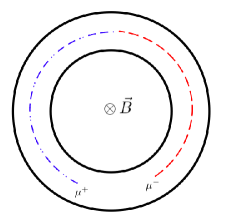
Figure 2: For a magnetic field $\vec{B}$ into the page, the positive muon $\mu^{+}$ follows the circle in blue (dot-dashed line), while the negative muon follows the red circle (dashed line).

We remark that the same device was also used in the recent experiment E821, carried out at the Brookhaven National Laboratory (whose final report can be found in [11]), which improved the precision of the CERN’s experiment. However, in addition to measuring the anomalous magnetic moment, the latter also focused on measuring the first clock effect through the dilation of the muon’s lifetime (which is not the case of E821, whose main idea was the measurement of the muon’s magnetic moment). For this reason we have chosen the CERN experiment as more appropriate for setting constraints on the second clock effect.

In what follows we will use Eq.(7) together with (4). As a first approximation, we will neglect the gravitational field of the Earth, and hence consider Minkowski space-time metric, written in cylindrical coordinates $\{t,\rho,\varphi,z\}$. The circular paths followed by the muons will be parametrized by the laboratory coordinate time $t$, while the initial conditions, the electromagnetic potential and the velocity will be chosen as

$$t_{0} =0,$$ (9a)

$$\left(\frac{d\tau/dt}{\sqrt{g_{\alpha\beta}\dot{x}^{\alpha}\dot{x}^{\beta}}}\right)_{t=t_{0}} =\frac{1}{c},$$ (9b)

$$A_{0} =0,$$ (9c)

$$\vec{A}(\rho) =-\frac{B}{2}\rho\hat{\varphi},$$ (9d)

$$\vec{v} =\pm v_{0}\hat{\varphi},$$ (9e)

where $$B \vec{\nabla}\times\vec{A}=\vec{B}=-B\,\hat{z} \rho_{0} v_{0} \vec{v}=\pm v_{0}\hat{\varphi} \mu^{\pm}$$ denotes the modulus of the magnetic field , is the radius of the circular trajectory, and is the constant norm of the velocity of the muons (here corresponds to the velocity of the muons , respectivelly).

Considering a first order expansion in the dimensionless argument of the exponential function from Eq.(7), and using definition (4), we approximate the proper time (7) as

$$\tau=\gamma^{-1}t-\lambda\,\frac{\gamma^{-1}}{2}\int_{0}^{t}\left(\int_{0}^{u}\vec{A}\cdot\vec{v}\,ds\right)du,$$ (10)

where $\gamma=\frac{1}{\sqrt{1-v_{0}^{2}/c^{2}}}$ is the Lorentz factor. Solving this equation for the above conditions and writing $v_{0}=c\sqrt{1-\gamma^{-2}}$, we obtain

$$\tau(\mu^{\pm})=\gamma^{-1}t(\mu^{\pm})\pm\lambda\frac{\gamma^{-1}}{8}c\rho_{0}B\sqrt{1-\gamma^{-2}}\,\left[t(\mu^{\pm})\right]^{2}.$$ (11)

In the above expression, $\tau(\mu^{\pm})$ is the decay time of the muons $\mu^{\pm}$ at rest (i.e., in its proper frame) and $t$ is their decay time in the laboratory frame. By solving the above equation for $t$, the dilated lifetime $t^{W}$ of the muons, due to Weyl geometry, will be given by

$$t^{W}(\mu^{\pm})=t^{\text{SR}}(\mu^{\pm})\mp\frac{\lambda}{8}c\rho_{0}B\sqrt{1-\gamma^{-2}}\left[t^{\text{SR}}(\mu^{\pm})\right]^{2},$$ (12)

where we have set $t^{\text{SR}}(\mu^{\pm})\doteq\gamma\tau(\mu^{\pm})$ to indicate the dilated lifetime of the muons, due only to special relativistic effects, i.e., to the first clock effect. We now see that the magnitude of the effect increases with the intensity of the magnetic field, the radius of the trajectory, the value of the Lorentz factor and (quadratically) with the dilated lifetime.

The parameters of the experiment are

$$B =1.472\,\text{T},$$ (13a)

$$\rho_{0} =7.00\,\text{m},$$ (13b)

$$\gamma \approx 29.327.$$ (13c)

Let us note that the above Lorentz factor used in CERN [12] and in the E821 experiment [11] is called magic $$\gamma t^{\text{EXP}}(\mu^{\pm}) t^{\text{SR}}(\mu^{\pm}) \sim 0.1\%$$, and it is the one that removes the contribution of the stabilizing quadrupole electrostatic field from the muon’s relation between the angular frequency and the electromagnetic field, named Thomas-Bargmann-Michel-Telegdi equation [13]. The values of the dilated lifetime of the muons, obtained in the experiment mentioned above are slightly different from the theoretical values predicted by special relativity with a precision of [12]:

$$t^{\text{EXP}}(\mu^{-}) \approx 64.368\,\mu\text{s},$$ (14a)

$$t^{\text{SR}}(\mu^{-}) \approx 64.461\,\mu\text{s},$$ (14b)

and

$$t^{\text{EXP}}(\mu^{+}) \approx 64.419\,\mu\text{s},$$ (15a)

$$t^{\text{SR}}(\mu^{+}) \approx 64.431\,\mu\text{s}.$$ (15b)

For $$\mu^{+} \mu^{-} t^{\text{SR}}(\mu^{\pm})=\gamma\tau(\mu^{\pm}) \tau(\mu^{\pm})$$ and there were two and four runs respectively, and what we have presented here is the average of the results. For the calculation of , we considered as given as in ref. [12], which had already been measured  (see [14, 15]).

It is important to remark that the experimentally measured decay times are distorted by statistical error and systematic effects (described in [12, 16]), such as the loss of muons from the trapping region before decay, variation of the decay electron detection efficiency (gain effects) and protons that may be stored in the ring, which contribute to background in the detectors (this effect is significant just for the $\mu^{+}$ decay time).

Let us now look at the difference between the decay times of the different muons $\Delta t=t^{\text{SR}}-t^{\text{EXP}}$

$$\Delta t(\mu^{+}) =0.012\,\mu\text{s},$$ (16)

$$\Delta t(\mu^{-}) =0.093\,\mu\text{s},$$ (17)

Statistical error and systematic contributions distort the detected lifetime of the particles. The negative muon $\mu^{-}$ seems to have a smaller detected decay time than $\mu^{+}$ does, which may be caused by a major contribution of systematic effects. But since we are also considering the possibility of the second clock effect, it seems reasonable to suppose that it contributes to the difference between $\mu^{-}$ and $\mu^{+}$. In this way, it seems plausible to consider that the non-metricity is diminishing the lifetime of $\mu^{-}$ and increasing of $\mu^{+}$ (which is compensated by the statistical error and systematic effects). This situation occurs if $\lambda<0$. Assuming this scenario we can use the expression (12) for $\mu^{-}$ to find a constraint.

Let us separate the detected decay time as follows

$$t^{\text{EXP}}=t^{\text{THE}}-t^{\text{ERR}},$$ (18)

where $t^{\text{THE}}$ is the theoretically predicted decay time, which in our case is given by $t^{\text{W}}$ in Eq.(12); and $t^{\text{ERR}}\geq 0$ is the contribution due to statistical error plus systematic effects of the experiment for each type of muon. Thus, we have the following inequality:

$$|\lambda|=8\frac{\Delta t(\mu^{-})-t^{\text{ERR}}}{c\rho_{0}B\sqrt{1-\gamma^{-2}}\left[t^{\text{SR}}(\mu^{-})\right]^{2}}\leq 8\frac{\Delta t(\mu^{-})}{c\rho_{0}B\sqrt{1-\gamma^{-2}}\left[t^{\text{SR}}(\mu^{-})\right]^{2}}\,,$$ (19)

which implies, using the above data (13), the following constraint in the CGS system of units:

$$|\lambda|\leq 5.81\times 10^{-16}\,\text{G}^{-1}\text{cm}^{-2}.$$ (20)

The same order of magnitude would have been found if we had considered $\mu^{+}$ for the analysis. Therefore, if there exists a second clock effect caused by Perlick’s proper time, then the Weyl parameter $\lambda$ should not exceed the constraint, i.e., we can estimate an upper bound given by

$$|\lambda|\lessapprox\mathcal{O}(10^{-16})\,\text{G}^{-1}\text{cm}^{-2}.$$ (21)

In this experiment we have all the ingredients for setting an unprecedented constraint on the possible existence of the second clock effect. Let us note that we have followed a conservative approach in the sense that if the Weyl parameter $\lambda$ does not surpass the order of magnitude (21), then the existence of the effect cannot be ruled out.

3.1 Phenomenological possibilities

Phenomenologically we can draw some scenarios we could expect to appear in future experiments. For instance, suppose that $\lambda$ is a parameter that depends on the electric charge of the particle that probes the space-time, i.e., there exists a $\lambda_{+}$ and a $\lambda_{-}$.

$1)$  The scenario in which $\lambda_{+}=\lambda_{-}=\lambda$ is suitable for this experiment, since Eq.(12) implies that the different types of muons, i.e., with different charges $\mu^{+}$ and $\mu^{-}$, when accelerated by a magnetic field will present different decay times. In other words, if systematic effects equivalently affect the experiment for both types of particles, then $\Delta t(\mu^{-})$ should be different than $\Delta t(\mu^{+})$ (assuming the existence of the second clock effect). Moreover, future experiments measuring dilated lifetimes, would indicate a tendency of increase in the quantity $|D_{\pm}|$ that we define below:

$$D_{\pm}=\Delta t(\mu^{-})-\Delta t(\mu^{+})$$ (22)

$2)$  If $\lambda_{+}\neq\lambda_{-}$ we should see a different pattern for $|D_{\pm}|$. For instance, if $\lambda_{+}=-\lambda_{-}$, then we should observe a decrease in $|D_{\pm}|$.

If we define $\Delta t^{\text{ERR}}\doteq t^{\text{ERR}}(\mu^{-})-t^{\text{ERR}}(\mu^{+})$,  then we can get rid of these effects by considering the following analysis for the two different scenarios cited above:

$$1)\ \lambda_{-}=\lambda_{+}=\lambda,\text{which leads to}$$

$$D_{\pm}=\Delta t^{\text{ERR}}-\frac{\lambda}{8}c\rho_{0}B\sqrt{1-\gamma^{-2}}\left[\left(t^{\text{SR}}(\mu^{-})\right)^{2}+\left(t^{\text{SR}}(\mu^{+})\right)^{2}\right],$$ (23)

$$2)\ \lambda_{-}=-\lambda_{+}=\lambda,\text{which gives}$$

$$D_{\pm}=\Delta t^{\text{ERR}}-\frac{\lambda}{8}c\rho_{0}B\sqrt{1-\gamma^{-2}}\left[\left(t^{\text{SR}}(\mu^{-})\right)^{2}-\left(t^{\text{SR}}(\mu^{+})\right)^{2}\right].$$ (24)

We expect $\Delta t^{\text{ERR}}$ to be a small quantity that should reduce even more with the improvement of the experiments. In any case, we can set a constraint on the parameter $\lambda$ for the two scenarios

$$|\lambda_{1,2}|\lessapprox 8\frac{|\Delta t(\mu^{-})-\Delta t(\mu^{+})|}{c\rho_{0}B\sqrt{1-\gamma^{-2}}}\left|\left(t^{\text{SR}}(\mu^{-})\right)^{2}\pm\left(t^{\text{SR}}(\mu^{+})\right)^{2}\right|^{-1}.$$ (25)

Using the above data (13), we find

$$|\lambda_{1}|\lessapprox 2.53\times 10^{-16}\,\text{G}^{-1}\text{cm}^{-2},$$ (26)

$$|\lambda_{2}|\lessapprox 5.44\times 10^{-13}\,\text{G}^{-1}\text{cm}^{-2}.$$ (27)

Since in the second scenario the contributions from the deformed proper time for $\mu^{+}$ and $\mu^{-}$ compensate each other, the constraint is less stringent than the one coming from the first scenario, which is of the same order of magnitude as (21).

4 Final remarks

By analyzing data obtained in an experiment carried out in CERN which measured the dilated lifetime of muons in a magnetic field we were able to set constraints on the existence of the second clock effect. More specifically, in terms of the parameter $\lambda$ we found that

$$|\lambda|\lessapprox\mathcal{O}(10^{-16})\,\text{G}^{-1}\text{cm}^{-2}.$$ (28)

Within the limits of experimental accuracy, we are allowed to consider the second clock effect as being responsible for an extra contribution to the particle’s dilated lifetime, in addition to the one coming from the first clock effect.

Finally, we would like to call attention for some phenomenological possibilities that could be addressed in future experiments, for instance the one to be carried out in Fermilab [17, 18, 19], which is expected to be operating in the near future. We also mention here the J-PARC experiment [20, 21], which although uses a different technique for the measurements of the anomalous magnetic moment of the muon, could also be of interest for testing the second clock effect.

References

- [1] For a review see, for instance, T. Clifton, P. G. Ferreira, A. Padilla, C. Skordis, Modified Gravity and Cosmology Phys. Rept. 513, 1, 1-189 (2012), doi: 10.1016/j.physrep.2012.01.001.
- [2] H. Weyl, “Gravitation und Elektrizität,” Sitzungsber. Preuss. Akad. Berlin. 465 - 480 (1918), also as a chapter in the book Das Relativitätsprinzip, English translation at http://www.tgeorgiev.net/Gravitation_and_Electricity.pdf.
- [3] L. O’Raifeartaigh and N. Straumann, “Early history of gauge theories and Kaluza-Klein theories,” hep-ph/9810524. L. O’Raifeartaigh, “The dawning of gauge theories” (Princeton University Press, 1997).
- [4] It seems that the expression second clock effect was first used in H. R. Brown and O. Pooley, “The origin of the spacetime metric: Bell’s ‘Lorentzian pedagogy’ and its significance in general relativity” in Physics meets Philosophy at the Planck Scale, C. Callender and N. Huggett (eds.), Cambridge University Press (2000).
- [5] See, for instance, C. Romero, “Is Weyl unified theory wrong or incomplete?,” arXiv:1508.03766 [gr-qc]. P. Teyssandier, R. W. Tucker and C. Wang, ”On an interpretation of non-Riemannian gravitation, Acta Phys. Pol. B 29, 987 (1998).
- [6] C. Barceló, R. Carballo-Rubio and L. J. Garay, “Weyl relativity: A novel approach to Weyl’s ideas,” JCAP 1706, no. 06, 014 (2017) doi:10.1088/1475-7516/2017/06/014 [arXiv:1703.06355 [gr-qc]].
- [7] V. Perlick, “Characterization of standard clocks by means of light rays and freely falling particles,” Gen. Relativ. Gravit. 19, 1059 (1987).
- [8] R. Avalos, F. Dahia and C. Romero, “A note on the problem of proper time in Weyl space-time,” Found. Phys. 48, 253 (2018).
- [9] J. Ehlers, F. A. E. Pirani and A. Schild, “Republication of: The geometry of free fall and light propagation,” Gen. Rel. Grav. 44, 1578 (2012).
- [10] J. Bailey et al. [CERN-Mainz-Daresbury Collaboration], “Final Report on the CERN Muon Storage Ring Including the Anomalous Magnetic Moment and the Electric Dipole Moment of the Muon, and a Direct Test of Relativistic Time Dilation,” Nucl. Phys. B 150, 1 (1979). doi:10.1016/0550-3213(79)90292-X
- [11] G. W. Bennett et al. [Muon g-2 Collaboration], “Final Report of the Muon E821 Anomalous Magnetic Moment Measurement at BNL,” Phys. Rev. D 73, 072003 (2006) doi:10.1103/PhysRevD.73.072003 [hep-ex/0602035].
- [12] J. Bailey et al., “Measurements of Relativistic Time Dilatation for Positive and Negative Muons in a Circular Orbit,” Nature 268, 301 (1977). doi:10.1038/268301a0
- [13] F. Jegerlehner, “The anomalous magnetic moment of the muon,” Springer Tracts Mod. Phys. 2nd edn. (Springer International Publishing AG, Gewerbestrasse, Switzerland, 2017).
- [14] M. P. Balandin, V. M. Grebenyuk, V. G. Zinov, A. D. Konin and A. N. Ponomarev, “Measurement of the Lifetime of the Positive Muon,” Sov. Phys. JETP 40, 811 (1975).
- [15] M. E. Nordberg, Jr., F. Lobkowicz and R. L. Burman, “Remeasurement of the Lifetime,” Phys. Lett. 24B, 594 (1967). doi:10.1016/0370-2693(67)90401-7
- [16] F. J. M. Farley and E. Picasso, “The Muon () Experiments at CERN,” Ann. Rev. Nucl. Part. Sci. 29, 243 (1979). doi:10.1146/annurev.ns.29.120179.001331
- [17] J. Grange et al. [Muon g-2 Collaboration], “Muon (g-2) Technical Design Report,” arXiv:1501.06858 [physics.ins-det].
- [18] D. W. Hertzog, “Next Generation Muon Experiments,” EPJ Web Conf. 118, 01015 (2016) doi:10.1051/epjconf/201611801015 [arXiv:1512.00928 [hep-ex]].
- [19] G. Venanzoni [Fermilab E989 Collaboration], “The New Muon g-2 experiment at Fermilab,” Nucl. Part. Phys. Proc. 273-275, 584 (2016) doi:10.1016/j.nuclphysbps.2015.09.087 [arXiv:1411.2555 [physics.ins-det]].
- [20] N. Saito [J-PARC g-2/EDM Collaboration], “A novel precision measurement of muon g-2 and EDM at J-PARC,” AIP Conf. Proc. 1467, 45 (2012). doi:10.1063/1.4742078
- [21] Y. Sato [E34 Collaboration], “Muon g-2/EDM experiment at J-PARC,” PoS KMI 2017, 006 (2017).