Unphysical Discontinuities in GW Methods

Abstract

We report unphysical irregularities and discontinuities in some key experimentally-measurable quantities computed within the GW approximation of many-body perturbation theory applied to molecular systems. In particular, we show that the solution obtained with partially self-consistent GW schemes depends on the algorithm one uses to solve self-consistently the quasi-particle (QP) equation. The main observation of the present study is that each branch of the self-energy is associated with a distinct QP solution, and that each switch between solutions implies a significant discontinuity in the quasiparticle energy as a function of the internuclear distance. Moreover, we clearly observe “ripple” effects, i.e., a discontinuity in one of the QP energies induces (smaller) discontinuities in the other QP energies. Going from one branch to another implies a transfer of weight between two solutions of the QP equation. The case of occupied, virtual and frontier orbitals are separately discussed on distinct diatomics. In particular, we show that multisolution behavior in frontier orbitals is more likely if the HOMO-LUMO gap is small.

1 Background

Many-body perturbation theory methods based on the one-body Green function $G$ are fascinating as they are able to transform an unsolvable many-electron problem into a set of non-linear one-electron equations, thanks to the introduction of an effective potential $\Sigma$, the self-energy. Electron correlation is explicitly incorporated via a sequence of self-consistent steps connected by Hedin’s equations. ¹ In particular, Hedin’s approach uses a dynamically screened Coulomb interaction $W$ instead of the standard bare Coulomb interaction. Important experimental properties such as ionization potentials, electron affinities as well as spectral functions, which are related to direct and inverse photo-emission, can be obtained directly from the one-body Green function. ² A particularly successful and practical approximation to Hedin’s equations is the so-called GW approximation ^{2, 3, 4} which bypasses the calculation of the most complicated part of Hedin’s equations, the vertex function. ¹

Although (perturbative) G₀W₀ is probably the simplest and most widely used GW variant, ^{5, 6, 7, 8, 9, 10} its starting point dependence has motivated the development of partially ^{11, 12, 13, 14, 15, 16, 17, 18, 19} and fully ^{20, 21, 22, 23, 24, 25, 26, 27, 28} self-consistent versions in order to reduce or remove this undesirable feature. Here, we will focus our attention on partially self-consistent schemes as they have demonstrated comparable accuracy and are computationally lighter than the fully self-consistent version. ²⁹ Moreover, they are routinely employed for solid-state and molecular calculations and are available in various computational packages. ^{13, 30, 31, 6, 32, 19, 33, 29, 34} Recently, an ever-increasing number of successful applications of partially self-consistent GW methods have sprung in the physics and chemistry literature for molecular systems, ^{18, 7, 8, 35, 31, 36, 27, 37, 30, 38, 39, 40, 37, 41, 9, 10} as well as extensive and elaborate benchmark sets. ^{9, 34, 10, 42, 43, 44, 45, 35, 46}

There exist two main types of partially self-consistent GW methods: i) “eigenvalue-only quasiparticle” GW (evGW), ^{11, 12, 13, 14} where the quasiparticle (QP) energies are updated at each iteration, and ii) “quasiparticle self-consistent” GW (qsGW), ^{15, 16, 17, 18, 19} where one updates both the QP energies and the corresponding orbitals. Note that a starting point dependence remains in evGW as the orbitals are not self-consistently optimized in this case.

In a recent article, ⁴⁷ while studying a model two-electron system, ^{48, 49, 50, 51, 52, 53} we have observed that, within partially self-consistent GW (such as evGW and qsGW), one can observe, in the weakly correlated regime, (unphysical) discontinuities in the energy surfaces of several key quantities (ionization potential, electron affinity, HOMO-LUMO gap, total and correlation energies, as well as vertical excitation energies). In the present manuscript, we provide further evidences and explanations of this undesirable feature in real molecular systems. For sake of simplicity, the present study is based on simple closed-shell diatomics (H2, F2 and BeO). However, the same phenomenon can be observed in many other molecular systems, such as LiF, HeH+, LiH, BN, O3, etc. Although we mainly focus on G₀W₀ and evGW, similar observations can be made in the case of qsGW and second-order Green function (GF2) methods. ^{54, 55, 56, 57, 58, 59, 60, 61, 62, 63, 64, 47} Unless otherwise stated, all calculations have been performed with our locally-developed GW software, which closely follows the MOLGW implementation. ³¹

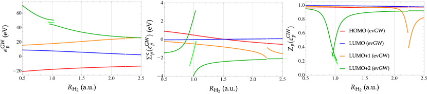
Figure 1: QP energies (left), correlation part of the self-energy (center) and renormalization factor (right) as functions of the internuclear distance $R_{\ce{H2}}$ for various orbitals of H2 at the G₀W₀@HF/6-31G (top) and evGW@HF/6-31G (bottom) levels. For convenience, the intermediate (center) branch is presented in lighter green for the LUMO+2.

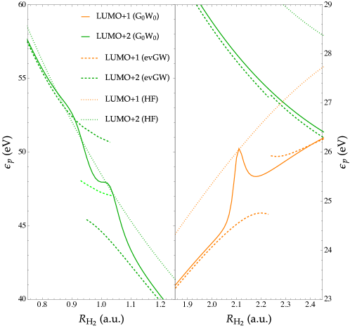
Figure 2: HF orbital energies (dotted lines) and QP energies as functions of the internuclear distance $R_{\ce{H2}}$ for the LUMO+1 and LUMO+2 orbitals of H2 at the G₀W₀@HF/6-31G (solid lines) and evGW@HF/6-31G (dashed lines) levels. For convenience, the intermediate (center) branch is presented in lighter green for the LUMO+2.

2 Theory

Here, we provide brief details about the main equations and quantities behind G₀W₀ and evGW considering a (restricted) Hartree-Fock (HF) starting point. ⁵⁴ More details can be found, for example, in Refs. 6, 19, 31.

For a given (occupied or virtual) orbital $p$, the correlation part of the self-energy is conveniently split in its hole (h) and particle (p) contributions

$$\Sigma^{\text{c}}_{p}(\omega)=\Sigma^{\text{p}}_{p}(\omega)+\Sigma^{\text{h}}_{p}(\omega),$$ (1)

which, within the GW approximation, read

$$\Sigma^{\text{h}}_{p}(\omega) =2\sum_{i}^{\text{occ}}\sum_{x}\frac{[pi|x]^{2}}{\omega-\epsilon_{i}+\Omega_{x}-i\eta},$$ (2a)

$$\Sigma^{\text{p}}_{p}(\omega) =2\sum_{a}^{\text{virt}}\sum_{x}\frac{[pa|x]^{2}}{\omega-\epsilon_{a}-\Omega_{x}+i\eta},$$ (2b)

where $\eta$ is a positive infinitesimal. The screened two-electron integrals

$$[pq|x]=\sum_{ia}(pq|ia)(\boldsymbol{X}+\boldsymbol{Y})_{ia}^{x}$$ (3)

are obtained via the contraction of the bare two-electron integrals ⁶⁵ $(pq|rs)$ and the transition densities $(\boldsymbol{X}+\boldsymbol{Y})_{ia}^{x}$ originating from a random phase approximation (RPA) calculation ^{66, 67}

$$\begin{pmatrix}\boldsymbol{A}&\boldsymbol{B}\\ \boldsymbol{B}&\boldsymbol{A}\\ \end{pmatrix}\begin{pmatrix}\boldsymbol{X}\\ \boldsymbol{Y}\\ \end{pmatrix}=\boldsymbol{\Omega}\begin{pmatrix}\boldsymbol{1}&\boldsymbol{0}\\ \boldsymbol{0}&\boldsymbol{-1}\\ \end{pmatrix}\begin{pmatrix}\boldsymbol{X}\\ \boldsymbol{Y}\\ \end{pmatrix},$$ (4)

with

$$A_{ia,jb} =\delta_{ij}\delta_{ab}(\epsilon_{a}-\epsilon_{i})+2(ia|jb), B_{ia,jb} =2(ia|bj),$$ (5)

and $\delta_{pq}$ is the Kronecker delta. ⁶⁸ The one-electron energies $\epsilon_{p}$ in (2a), (2b) and (5) are either the HF or the GW quasiparticle energies. Equation (4) also provides the neutral excitation energies $\Omega_{x}$.

In practice, there exist two ways of determining the G₀W₀ QP energies. ^{5, 6} In its “graphical” version, they are provided by one of the many solutions of the (non-linear) QP equation

$$\omega=\epsilon^{\text{HF}}_{p}+\real[\Sigma^{\text{c}}_{p}(\omega)].$$ (6)

In this case, special care has to be taken in order to select the “right” solution, known as the QP solution. In particular, it is usually worth calculating its renormalization weight (or factor), $Z_{p}(\epsilon^{\text{HF}}_{p})$, where

$$Z_{p}(\omega)=\quantity[1-\partialderivative{\real[\Sigma^{\text{c}}_{p}(\omega)]}{\omega}]^{-1}.$$ (7)

Because of sum rules, ^{69, 70, 71, 72} the other solutions, known as satellites, share the remaining weight. In a well-behaved case (belonging to the weakly correlated regime), the QP weight is much larger than the sum of the satellite weights, and of the order of $0.7$-$0.9$.

Within the linearized version of G₀W₀, one assumes that

$$\Sigma^{\text{c}}_{p}(\omega)\approx\Sigma^{\text{c}}_{p}(\epsilon^{\text{HF}}_{p})+(\omega-\epsilon^{\text{HF}}_{p})\left.\partialderivative{\Sigma^{\text{c}}_{p}(\omega)}{\omega}\right|_{\omega=\epsilon^{\text{HF}}_{p}},$$ (8)

that is, the self-energy behaves linearly in the vicinity of $\omega=\epsilon^{\text{HF}}_{p}$. Substituting (8) into (6) yields

$$\epsilon^{\text{G${}_{0}$W${}_{0}$}}_{p}=\epsilon^{\text{HF}}_{p}+Z_{p}(\epsilon^{\text{HF}}_{p})\real[\Sigma^{\text{c}}_{p}(\epsilon^{\text{HF}}_{p})].$$ (9)

Unless otherwise stated, in the remaining of this paper, the G₀W₀ QP energies are determined via the linearized method.

In the case of evGW, the QP energy, $\epsilon^{\text{GW}}_{p}$, are obtained via Eq. (6), which has to be solved self-consistently due to the QP energy dependence of the self-energy [see Eq. (1)]. ^{11, 12, 13, 14} At least in the weakly correlated regime where a clear QP solution exists, we believe that, within evGW, the self-consistent algorithm should select the solution of the QP equation (6) with the largest renormalization weight $Z_{p}(\epsilon^{\text{GW}}_{p})$. In order to avoid convergence issues, we have used the DIIS convergence accelerator technique proposed by Pulay. ^{73, 74} Details about our implementation of DIIS for evGW can be found in the Appendix. Moreover, throughout this paper, we have set $\eta=0$.

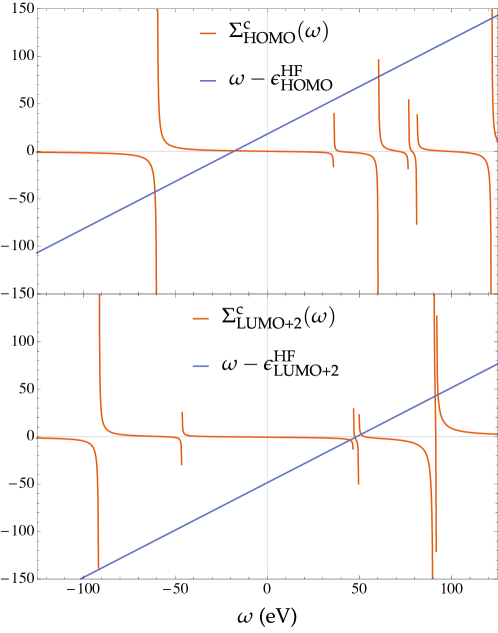
Figure 3: $\Sigma^{\text{c}}_{\text{HOMO}}(\omega)$ and $\Sigma^{\text{c}}_{\text{LUMO}+2}(\omega)$ (in eV) as functions of the frequency $\omega$ obtained at the evGW@HF/6-31G level for H2 at $R_{\ce{H2}}=1.0$ bohr. The solutions of the QP equation are given by the intersection of the orange and blue curves.

3 Results

3.1 Virtual orbitals

As a first example, we consider the hydrogen molecule H2 in a relatively small gaussian basis set (6-31G) in order to be able to study easily the entire orbital energy spectrum. Although the number of irregularities/discontinuities as well as their locations may vary with the basis set, the conclusions we are going to draw here are general.

Figure 1 reports three key quantities as functions of the internuclear distance $R_{\ce{H2}}$ for various orbitals at the G₀W₀ and the self-consistent evGW levels: i) the QP energies [$\epsilon^{\text{G${}_{0}$W${}_{0}$}}_{p}$ or $\epsilon^{\text{GW}}_{p}$], ii) the correlation part of the self-energy [$\Sigma^{\text{c}}_{p}(\epsilon^{\text{HF}}_{p})$ or $\Sigma^{\text{c}}_{p}(\epsilon^{\text{GW}}_{p})$], and iii) the renormalization factor/weight [$Z_{p}(\epsilon^{\text{HF}}_{p})$ or $Z_{p}(\epsilon^{\text{GW}}_{p})$].

3.1.1 G₀W₀

Let us first consider the results of the G₀W₀ calculations reported in the top row of Fig. 1. Looking at the curves of $\epsilon^{\text{G${}_{0}$W${}_{0}$}}_{p}$ as a function of $R_{\ce{H2}}$ (top left graph of Fig. 1), one notices obvious irregularities in the LUMO+2 around $R_{\ce{H2}}=1.0$ bohr and in the LUMO+1 around $R_{\ce{H2}}=2.1$ bohr. For information, the experimental equilibrium geometry of H2 is around $R_{\ce{H2}}=1.4$ bohr. ⁷⁵ These irregularities are unphysical, and occur in correspondence with a series of poles in $\Sigma^{\text{c}}_{\text{LUMO}+1}$ and $\Sigma^{\text{c}}_{\text{LUMO}+2}$ (see top center graph of Fig. 1). For example, one can notice two poles in $\Sigma^{\text{c}}_{\text{LUMO}+2}$ just before and after $R_{\ce{H2}}=1.0$ bohr, giving birth to three branches. The origin of the irregularities in $\epsilon_{\text{LUMO}+1}$ and $\epsilon_{\text{LUMO}+2}$ can, therefore, be traced back to the wrong assumption that $\Sigma^{\text{c}}_{\text{LUMO}+1}(\omega)$ and $\Sigma^{\text{c}}_{\text{LUMO}+2}(\omega)$ are linear functions of $\omega$ in the vicinity of, respectively, $\omega=\epsilon^{\text{HF}}_{\text{LUMO}+1}$ and $\omega=\epsilon^{\text{HF}}_{\text{LUMO}+2}$ [see Eq. (8)].

However, despite the divergencies in the self-energy, the QP energies $\epsilon^{\text{G${}_{0}$W${}_{0}$}}_{\text{LUMO}+1}$ and $\epsilon^{\text{G${}_{0}$W${}_{0}$}}_{\text{LUMO}+2}$ remain finite thanks to a rapid decrease of the renormalization factor at the $R_{\ce{H2}}$ values for which the self-energy diverges [see Eq. (6) and top right graph of Fig. 1]. For example, note that $Z_{\text{LUMO}+2}$ reaches exactly zero at the pole locations. A very similar scenario unfolds for the LUMO+1, except that a single pole is present in $\Sigma^{\text{c}}_{\text{LUMO}+1}$.

Let us analyze this point further. Since the self-energy behaves as $\Sigma^{\text{c}}_{p}\sim\delta^{-1}$ (with $\delta\to 0$) in the vicinity of a singularity, one can easily show that $Z_{p}\sim(1+\delta^{-2})^{-1}\sim\delta^{2}$, which yields $\epsilon^{\text{G${}_{0}$W${}_{0}$}}_{p}\sim\epsilon^{\text{HF}}_{p}+\delta$. In plain words, $\epsilon^{\text{G${}_{0}$W${}_{0}$}}_{p}$ remains finite near the poles of the self-energy thanks to the linearization of the QP equation [see Eq. (6)]. It also evidences that, at the pole locations (i.e. $\delta=0$), we have $\epsilon^{\text{G${}_{0}$W${}_{0}$}}_{p}=\epsilon^{\text{HF}}_{p}$, i.e., by construction the QP energy is forced to remain equal to the zeroth-order energy. This is nicely illustrated in Fig. 2, where we have plotted the HF orbital energies (dotted lines) as well as the G₀W₀ QP energies (solid lines) around the two “problematic” internuclear distances. The behavior of $\epsilon^{\text{G${}_{0}$W${}_{0}$}}_{\text{LUMO}+1}$ (solid orange line on the right panel of Fig. 2) is particularly instructive and shows that the G₀W₀ QP energies can have an erratic behavior near the poles of the self-energy.

It is interesting to investigate further the origin of these poles. As evidenced by Eq. (1), for a calculation involving $2n$ electrons and $N$ basis functions, the self-energy has exactly $nN(N-n)$ poles originating from the combination of the $N$ poles of the Green function $G$ (at frequencies $\epsilon_{p}$) and the $n(N-n)$ poles of the screened Coulomb interaction $W$ (at the RPA singlet excitations $\Omega_{x}$). For example, at $R_{\ce{H2}}=2.11$ bohr, the combination of $\epsilon^{\text{HF}}_{\text{LUMO}}=3.83$ eV and the HOMO-LUMO-dominated first neutral excitation energy $\Omega_{1}=22.24$ eV are equal to the LUMO+1 energy $\epsilon^{\text{G${}_{0}$W${}_{0}$}}_{\text{LUMO}+1}=26.07$ eV. Around $R_{\ce{H2}}=1.0$ bohr, the two poles of $\Sigma^{\text{c}}_{\text{LUMO}+1}$ are due to the following accidental equalities: $\epsilon^{\text{G${}_{0}$W${}_{0}$}}_{\text{LUMO}+1}=\epsilon^{\text{HF}}_{\text{LUMO}}+\Omega_{2}$, and $\epsilon^{\text{G${}_{0}$W${}_{0}$}}_{\text{LUMO}+1}=\epsilon^{\text{HF}}_{\text{LUMO}+1}+\Omega_{1}$. Because the number of poles in $G$ and $W$ (at the non-interacting or HF level) are both proportional to $N$, these spurious poles in the self-energy become more and more frequent for larger gaussian basis sets. For virtual orbitals, the higher in energy the orbital is, the earlier the singularities seem to appear.

Finally, the irregularities in the G₀W₀ QP energies as a function of $R_{\ce{H2}}$ can also be understood as follows. Since within G₀W₀ only one pole of $G$ is calculated, i.e., the QP energy, all the satellite poles are discarded. Mixing between QP and satellites poles, which is important when they are close to each other, hence, is not considered. This situation can be compared to the lack of mixing between single and double excitations in adiabatic time-dependent density-functional theory and the Bethe-Salpeter equation ^{76, 77, 78, 79} (see also Refs. 80, 81, 82, 83).

3.1.2 evGW

Within partially self-consistent schemes, the presence of poles in the self-energy at a frequency similar to a QP energy has more dramatic consequences. The results for H2 at the evGW@HF/6-31G level are reported in the bottom row of Fig. 1. Around $R_{\ce{H2}}=1.0$ bohr, we observe that, for the LUMO+2, one can fall onto three distinct solutions depending on the algorithm one relies on to solve self-consistently the QP equation (see bottom left graph of Fig. 1). In order to obtain each of the three possible solutions in the vicinity of $R_{\ce{H2}}=1.0$ bohr, we have run various sets of calculations using different starting values for the QP energies and sizes of the DIIS space. In particular, we clearly see that each of these solutions yield a distinct energy separated by several electron volts (see zoom in Fig. 2), and each of them is associated with a well-defined branch of the self-energy, as shown by the center graph in the bottom row of Fig. 1. For convenience, the intermediate (center) branch is presented in lighter green in Figs. 1 and 2, while the left and right branches are depicted in darker green. Interestingly, the evGW iterations are able to “push” the QP solution away from the poles of the self-energy, which explains why the renormalization factor is never exactly equal to zero (see bottom right graph of Fig. 1). However, one cannot go smoothly from one branch to another, and each switch between solutions implies a significant energetic discontinuity. Moreover, we observe “ripple” effects in other virtual orbitals: a discontinuity in one of the QP energies induces (smaller) discontinuities in the others. This is a direct consequence of the global energy dependence of the self-energy [see Eq. (1)], and is evidenced on the left graph in the bottom row of Fig. 1 around $R_{\ce{H2}}=2.1$ bohr.

The main observation of the present study is that each branch of the self-energy is associated with a distinct QP solution. We clearly see that, when one goes from one branch to another, there is a transfer of weight between the QP and one of the satellites, which becomes the QP on the new branch. ⁴⁷ As opposed to the strongly correlated regime where the QP picture breaks down, i.e., there is no clear QP, here there is alway a clear QP except at the vicinity of the poles where the weight transfer occurs. As for G₀W₀, this sudden transfer is caused by the artificial removal of the satellite poles. However, in the evGW results the problem is amplified by the self-consistency. We expect that keeping the full frequency dependence of the self-energy would solve this problem.

It is also important to mention that the self-consistent algorithm is fairly robust as it rarely selects a solution with a renormalization weight lower than $0.5$, as shown by the center graph in the bottom row of Fig. 1. In other words, when the renormalization factor of the QP solution becomes too small, the self-consistent algorithm switches naturally to a different solution. From a technical point of view, around the poles of the self-energy, it is particularly challenging to converge self-consistent calculations, and we heavily relied on DIIS to avoid such difficulties. We note that an alternative ad hoc approach to stabilize such self-consistent calculations is to increase the value of the positive infinitesimal $\eta$.

Figure 3 shows the correlation part of the self-energy for the HOMO and LUMO+2 orbitals as a function of $\omega$ (orange curves) obtained at the self-consistent evGW@HF/6-31G level for H2 with $R_{\ce{H2}}=1.0$ bohr. The solutions of the QP equation (6) are given by the intersections of the orange and blue curves. On the one hand, in the case of the HOMO, we have an unambiguous QP solution (at $\omega\approx-20$ eV) which is well separated from the other solutions. In this case, one can anticipate a large value of the renormalization factor $Z_{\text{HOMO}}$ as the self-energy is flat around the intersection of the two curves. On the other hand, for the LUMO+2, we see three solutions of the QP equation very close in energy from each other around $\omega=50$ eV. In this particular case, there is no well-defined QP peak as each solution has a fairly small weight. Therefore, one may anticipate multiple solution issues when a solution of the QP equation is close to a pole of the self-energy.

Finally, we note that the multiple solutions discussed here are those of the QP equation, i.e., multiple QP poles associated to a single Green function. This is different from the multiple solutions discussed in Refs. 84, 85, 86, 87, 88, 89, 90, in which it is shown that, in general, the nonlinear Dyson equation admits multiple Green functions, which can be physical but also unphysical.

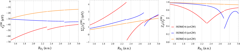
Figure 4: QP energies (left), correlation part of the self-energy (center) and renormalization factor (right) as functions of the internuclear distance $R_{\ce{F2}}$ for various occupied orbitals of F2 at the evGW@HF/STO-3G level.

3.2 Occupied orbitals

So far, we have seen that multiple solutions seem to only appear for virtual orbitals (LUMO excluded). However, we will show here that it can also happen in occupied orbitals. We take as an example the fluorine molecule (F2) in a minimal basis set (STO-3G), and perform evGW@HF calculations within the frozen-core approximation, that is, we do not update the orbital energies associated with the core orbitals. Figure 4 shows the behavior (as a function of the distance between the two fluorine atoms $R_{\ce{F2}}$) of the same quantities as in Fig. 1 but for some of the occupied orbitals of F2 (HOMO-6, HOMO-5 and HOMO-4). Similarly to the case of H2 discussed in the previous section, we see discontinuities in the QP energies around $R_{\ce{F2}}=2.3$ bohr (for the HOMO-6) and $R_{\ce{F2}}=2.7$ bohr (for the HOMO-5). For information, the experimental equilibrium geometry of F2 is $R_{\ce{F2}}=2.668$ bohr, which evidences that the second discontinuity is extremely close to the experimental geometry. Let us mention here that we have not found any discontinuity in the HOMO orbital. The case of the frontier orbitals will be discussed below. For F2, here again, we clearly observe ripple effects on other occupied orbitals. Similarly to virtual orbitals, we have found that the lower in energy the orbital is, the earlier the singularities seem to appear.

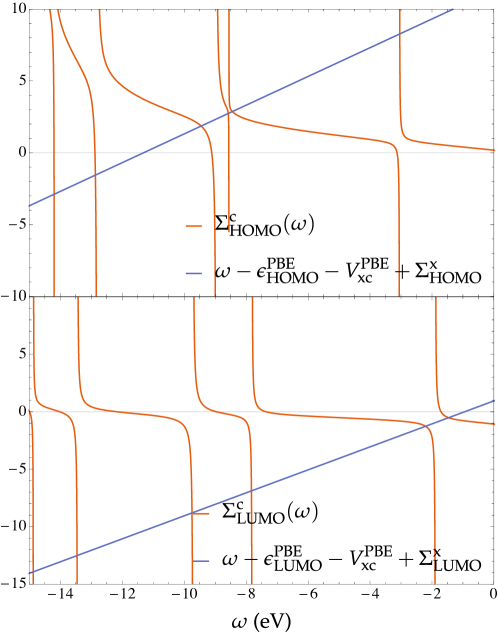
Figure 5: $\Sigma^{\text{c}}_{\text{HOMO}}(\omega)$ and $\Sigma^{\text{c}}_{\text{LUMO}}(\omega)$ (in eV) as functions of the frequency $\omega$ obtained at the G₀W₀@PBE/cc-pVDZ level for BeO at its experimental geometry. ⁷⁵ The solutions of the QP equations are given by the intersection of the orange and blue curves.

3.3 Frontier orbitals

Before concluding, we would like to know, whether or not, this multisolution behavior can potentially appear in frontier orbitals. This is an important point to discuss as these orbitals are directly related to the ionization potential and the electron affinity, hence to the gap.

Let us take the HOMO orbital as an example. A similar rationale holds for the LUMO orbital. According to the expression of the hole and particle parts of the self-energy given in Eqs. (2a) and (2b) respectively, $\Sigma^{\text{c}}_{\text{HOMO}}(\omega)$ has poles at $\omega=\epsilon_{i}-\Omega_{x}$ and $\omega=\epsilon_{a}+\Omega_{x}$ with $\Omega_{x}>0$. Evaluating the self-energy at $\omega=\epsilon_{\text{HOMO}}$ would yield $\epsilon_{\text{HOMO}}-\epsilon_{i}=-\Omega_{x}$ and $\epsilon_{\text{HOMO}}-\epsilon_{a}=+\Omega_{x}$, which is in clear contradiction with the assumption that $\Omega_{x}>0$. Therefore, the self-energy is never singular at $\omega=\epsilon_{\text{HOMO}}$ and $\omega=\epsilon_{\text{LUMO}}$ and the linearized G₀W₀ equations can be solved without any problem for the frontier orbitals. This is true for any $G_{0}$, that is, it does not depend on the starting point. As can be seen from Eqs. (2a) and (2b), the two poles of the self-energy closest to the Fermi level are located at $\omega=\epsilon_{\text{HOMO}}-\Omega_{1}$ and $\omega=\epsilon_{\text{LUMO}}+\Omega_{1}$. As a consequence, there is a region equal to $\epsilon_{\text{HOMO}}-\epsilon_{\text{LUMO}}+2\Omega_{1}$ around the Fermi level in which the self-energy does not have poles. Because $\Omega_{1}\approx\epsilon_{\text{HOMO}}-\epsilon_{\text{LUMO}}=E_{\text{gap}}$, this region is approximately equal to $3E_{\text{gap}}$.

For “graphical” G₀W₀, the solution might lie outside this range, even for the frontier orbitals. This can happen when $E_{\text{gap}}$ is much smaller than the true GW gap. In particular, this could occur for graphical G₀W₀ on top of a Kohn-Sham starting point, which is known to yield gaps that are (much) smaller than GW gaps. Within graphical G₀W₀, multiple solution issues for the HOMO have been reported by van Setten and coworkers ^{9, 34} in several systems (LiH, BN, BeO and O3). In their calculations, they employed PBE orbital energies ⁹¹ as starting point, and this type of functionals is well known to drastically underestimate $E_{\text{gap}}$. ⁹²

As an example, we have computed, within the frozen-core approximation, $\Sigma^{\text{c}}_{\text{HOMO}}(\omega)$ and $\Sigma^{\text{c}}_{\text{LUMO}}(\omega)$ as functions of $\omega$ at the G₀W₀@PBE/cc-pVDZ level for beryllium monoxide (BeO) at its experimental geometry (i.e. $R_{\ce{BeO}}=2.515$ bohr). ⁷⁵ These calculations have been performed with MOLGW. ³¹ The results are gathered in Fig. 5, where one clearly sees that multiple solutions appear for both the HOMO and LUMO orbitals. Note that performing the same set of calculations with a HF starting point yields a perfectly unambiguous single QP solution. For this system, PBE is a particularly bad starting point for a GW calculation with a HOMO-LUMO gap equal to $1.35$ eV. Using the same basis set, HF yields a gap of $8.96$ eV, while G₀W₀@HF and G₀W₀@PBE yields $7.54$ and $5.60$ eV. The same observations can be made for the other systems reported as problematic by van Setten and coworkers. ^{9, 34} As a general rule, it is known that HF is usually a better starting point for GW in small molecular systems. ^{13, 8, 47, 93} For larger systems, hybrid functionals ⁹⁴ might be the ideal compromise, thanks to the increase of the HOMO-LUMO gap via the addition of (exact) HF exchange. ^{8, 38, 35, 46, 95}

4 Concluding remarks

The GW approximation of many-body perturbation theory has been highly successful at predicting the electronic properties of solids and molecules. ^{2, 3, 4} However, it is also known to be inadequate to model strongly correlated systems. ^{96, 97, 98, 99, 87} Here, we have found severe shortcomings of two widely-used variants of GW in the weakly correlated regime. We have evidenced that one can hit multiple solution issues within G₀W₀ and evGW due to the location of the QP solution near poles of the self-energy. Within linearized G₀W₀, this implies irregularities in key experimentally-measurable quantities of simple diatomics, while, at the partially self-consistent evGW level, discontinues arise. Because the RPA correlation energy ^{66, 100, 101, 31} and the Bethe-Salpeter excitation energies ^{102, 103, 30} directly dependent on the QP energies, these types of discontinuities are also present in these quantities, hence in the energy surfaces of ground and excited states. Illustrative examples can be found in our previous study. ⁴⁷ We believe that such discontinuities would not exist within a fully self-consistent scheme where one does not iterate the QP energies but the one-body Green’s function and therefore takes into account each QP peak as well as its satellites at every iteration. Obviously, this latter point deserves further investigations. However, if confirmed, this would be a strong argument in favor of fully self-consistent schemes. Also, for extended systems, these issues might be mitigated by the plasmon modes that dominate the high-energy spectrum of the screened Coulomb interaction. The results of this work will be useful for self-consistent GW calculations of dynamical phenomena, i.e., with nuclear motion.

We are currently exploring different routes in order to remove these unphysical features. Padé resummation technique could be of great interest ¹⁰⁴ for such purpose. However, other techniques might be successful at alleviating this issue. For example, one could i) impose a larger offset from the real axis (i.e. increasing the value of $\eta$), ii) favor, in the case of small systems, a HF starting point in order to avoid small HOMO-LUMO gaps, or iii) rely, for larger systems, on hybrid functionals including a significant fraction of HF exchange. Also, regularization techniques, such as the one developed for orbital-optimized second-order Møller-Plesset perturbation theory, could be pragmatic and efficient way of removing such discontinuities. ¹⁰⁵

PFL would like to thank Xavier Blase and Fabien Bruneval for valuable discussions. The authors would like to thank Valerio Olevano for stimulating discussions during his sabbatical stay at IRSAMC. MV thanks Université Paul Sabatier (Toulouse, France) for a PhD scholarship.

Appendix: DIIS implementation for GW

DIIS (standing for “direct inversion of the iterative subspace”) is an extrapolation technique introduced by Pulay in 1980 ^{73, 74} in order to speed up the convergence of self-consistent HF calculations. The DIIS implementation for the evGW method is rather straightforward and reminiscent of the coupled cluster (CC) implementation. ¹⁰⁶ Within evGW, at iteration $n$, DIIS provides a set of normalized weight $\boldsymbol{w}$ in order to extrapolate the current values of the QP energies $\boldsymbol{\epsilon}^{\text{G${}_{n}$W${}_{n}$}}$ based on the $N^{\text{DIIS}}=\min(n-1,N_{\text{max}}^{\text{DIIS}})$ previous values, i.e.,

$$\boldsymbol{\epsilon}^{\text{G${}_{n}$W${}_{n}$}}=\sum_{m=1}^{N^{\text{DIIS}}}w_{m}\boldsymbol{\epsilon}^{\text{G${}_{n-m}$W${}_{n-m}$}},$$ (10)

where $N_{\text{max}}^{\text{DIIS}}$ is a user-defined parameter setting the maximum size of the DIIS space. This procedure only requires to store the QP energies $\boldsymbol{\epsilon}^{\text{G${}_{n}$W${}_{n}$}}$ at each iteration. The DIIS extrapolation technique relies on the fact that, at convergence, $\Delta\boldsymbol{\epsilon}^{\text{G${}_{n-1}$W${}_{n-1}$}}=\boldsymbol{\epsilon}^{\text{G${}_{n-1}$W${}_{n-1}$}}-\boldsymbol{\epsilon}^{\text{G${}_{n-2}$W${}_{n-2}$}}=\bm{0}$. Consequently, the weights are obtained by solving the linear system $\boldsymbol{A}\boldsymbol{w}=\boldsymbol{b}$, where

$$\boldsymbol{A}= \begin{pmatrix}(\Delta\boldsymbol{\epsilon}^{\text{G${}_{n-1}$W${}_{n-1}$}})^{\dagger}\,\Delta\boldsymbol{\epsilon}^{\text{G${}_{n-1}$W${}_{n-1}$}}&\cdots&(\Delta\boldsymbol{\epsilon}^{\text{G${}_{n-N^{\text{DIIS}}}$W${}_{n-N^{\text{DIIS}}}$}})^{\dagger}\,\Delta\boldsymbol{\epsilon}^{\text{G${}_{n-1}$W${}_{n-1}$}}&-1\\ \vdots&\ddots&\vdots&\vdots\\ (\Delta\boldsymbol{\epsilon}^{\text{G${}_{n-1}$W${}_{n-1}$}})^{\dagger}\,\Delta\boldsymbol{\epsilon}^{\text{G${}_{n-N^{\text{DIIS}}}$W${}_{n-N^{\text{DIIS}}}$}}&\cdots&(\Delta\boldsymbol{\epsilon}^{\text{G${}_{n-N^{\text{DIIS}}}$W${}_{n-N^{\text{DIIS}}}$}})^{\dagger}\,\Delta\boldsymbol{\epsilon}^{\text{G${}_{n-N^{\text{DIIS}}}$W${}_{n-N^{\text{DIIS}}}$}}&-1\\ -1&\cdots&-1&0\\ \end{pmatrix},$$ (11)

$$\boldsymbol{b}= \begin{pmatrix}0\\ \vdots\\ 0\\ -1\\ \end{pmatrix}.$$ (12)

When the linear system becomes ill-conditioned, we reset $N^{\text{DIIS}}=0$ and restart the DIIS extrapolation procedure. For $N_{\text{max}}^{\text{DIIS}}=2$, the present algorithm can be seen as an optimal linear mixing strategy, as usually implemented in other softwares. ^{19, 25} For qsGW, we have found that extrapolating the self-energy similarly to what is done for the Fock matrix in HF or KS methods is particularly efficient. ^{73, 74}

References

- Hedin 1965 Hedin, L. New Method for Calculating the One-Particle Green’s Function with Application to the Electron-Gas Problem. Phys. Rev. 1965, 139, A796
- Onida et al. 2002 Onida, G.; Reining, L.; and, A. R. Electronic excitations: density-functional versus many-body Green’s-function approaches. Rev. Mod. Phys. 2002, 74, 601–659
- Aryasetiawan and Gunnarsson 1998 Aryasetiawan, F.; Gunnarsson, O. The GW method. Rep. Prog. Phys. 1998, 61, 237–312
- Reining 2017 Reining, L. The GW Approximation: Content, Successes and Limitations: The GW Approximation. Wiley Interdiscip. Rev. Comput. Mol. Sci. 2017, e1344
- Hybertsen and Louie 1985 Hybertsen, M. S.; Louie, S. G. First-Principles Theory of Quasiparticles: Calculation of Band Gaps in Semiconductors and Insulators. Phys. Rev. Lett. 1985, 55, 1418–1421
- van Setten et al. 2013 van Setten, M. J.; Weigend, F.; Evers, F. The GW -Method for Quantum Chemistry Applications: Theory and Implementation. J. Chem. Theory Comput. 2013, 9, 232–246
- Bruneval 2012 Bruneval, F. Ionization Energy of Atoms Obtained from GW Self-Energy or from Random Phase Approximation Total Energies. J. Chem. Phys. 2012, 136, 194107
- Bruneval and Marques 2013 Bruneval, F.; Marques, M. A. L. Benchmarking the Starting Points of the GW Approximation for Molecules. J. Chem. Theory Comput. 2013, 9, 324–329
- van Setten et al. 2015 van Setten, M. J.; Caruso, F.; Sharifzadeh, S.; Ren, X.; Scheffler, M.; Liu, F.; Lischner, J.; Lin, L.; Deslippe, J. R.; Louie, S. G.; Yang, C.; Weigend, F.; Neaton, J. B.; Evers, F.; Rinke, P. GW 100: Benchmarking G 0 W 0 for Molecular Systems. J. Chem. Theory Comput. 2015, 11, 5665–5687
- van Setten et al. 2018 van Setten, M. J.; Costa, R.; Viñes, F.; Illas, F. Assessing GW Approaches for Predicting Core Level Binding Energies. J. Chem. Theory Comput. 2018, 14, 877–883
- Hybertsen and Louie 1986 Hybertsen, M. S.; Louie, S. G. Electron Correlation in Semiconductors and Insulators: Band Gaps and Quasiparticle Energies. Phys. Rev. B 1986, 34, 5390–5413
- Shishkin and Kresse 2007 Shishkin, M.; Kresse, G. Self-Consistent G W Calculations for Semiconductors and Insulators. Phys. Rev. B 2007, 75, 235102
- Blase et al. 2011 Blase, X.; Attaccalite, C.; Olevano, V. First-Principles GW Calculations for Fullerenes, Porphyrins, Phtalocyanine, and Other Molecules of Interest for Organic Photovoltaic Applications. Phys. Rev. B 2011, 83, 115103
- Faber et al. 2011 Faber, C.; Attaccalite, C.; Olevano, V.; Runge, E.; Blase, X. First-Principles GW Calculations for DNA and RNA Nucleobases. Phys. Rev. B 2011, 83, 115123
- Faleev et al. 2004 Faleev, S. V.; van Schilfgaarde, M.; Kotani, T. All-Electron Self-Consistent G W Approximation: Application to Si, MnO, and NiO. Phys. Rev. Lett. 2004, 93, 126406
- van Schilfgaarde et al. 2006 van Schilfgaarde, M.; Kotani, T.; Faleev, S. Quasiparticle Self-Consistent G W Theory. Phys. Rev. Lett. 2006, 96, 226402
- Kotani et al. 2007 Kotani, T.; van Schilfgaarde, M.; Faleev, S. V. Quasiparticle Self-Consistent G W Method: A Basis for the Independent-Particle Approximation. Phys. Rev. B 2007, 76, 165106
- Ke 2011 Ke, S.-H. All-Electron G W Methods Implemented in Molecular Orbital Space: Ionization Energy and Electron Affinity of Conjugated Molecules. Phys. Rev. B 2011, 84, 205415
- Kaplan et al. 2016 Kaplan, F.; Harding, M. E.; Seiler, C.; Weigend, F.; Evers, F.; van Setten, M. J. Quasi-Particle Self-Consistent GW for Molecules. J. Chem. Theory Comput. 2016, 12, 2528–2541
- Stan et al. 2006 Stan, A.; Dahlen, N. E.; van Leeuwen, R. Fully Self-Consistent GW Calculations for Atoms and Molecules. Europhys. Lett. EPL 2006, 76, 298–304
- Stan et al. 2009 Stan, A.; Dahlen, N. E.; van Leeuwen, R. Levels of Self-Consistency in the GW Approximation. J. Chem. Phys. 2009, 130, 114105
- Rostgaard et al. 2010 Rostgaard, C.; Jacobsen, K. W.; Thygesen, K. S. Fully Self-Consistent GW Calculations for Molecules. Phys. Rev. B 2010, 81, 085103
- Caruso et al. 2012 Caruso, F.; Rinke, P.; Ren, X.; Scheffler, M.; Rubio, A. Unified Description of Ground and Excited States of Finite Systems: The Self-Consistent G W Approach. Phys. Rev. B 2012, 86, 081102(R)
- Caruso et al. 2013 Caruso, F.; Rohr, D. R.; Hellgren, M.; Ren, X.; Rinke, P.; Rubio, A.; Scheffler, M. Bond Breaking and Bond Formation: How Electron Correlation Is Captured in Many-Body Perturbation Theory and Density-Functional Theory. Phys. Rev. Lett. 2013, 110, 146403
- Caruso et al. 2013 Caruso, F.; Rinke, P.; Ren, X.; Rubio, A.; Scheffler, M. Self-Consistent G W : All-Electron Implementation with Localized Basis Functions. Phys. Rev. B 2013, 88, 075105
- Caruso 2013 Caruso, F. Self-Consistent GW Approach for the Unified Description of Ground and Excited States of Finite Systems. PhD Thesis, Freie Universität Berlin, 2013
- Koval et al. 2014 Koval, P.; Foerster, D.; Sánchez-Portal, D. Fully Self-Consistent G W and Quasiparticle Self-Consistent G W for Molecules. Phys. Rev. B 2014, 89, 155417
- Wilhelm et al. 2018 Wilhelm, J.; Golze, D.; Talirz, L.; Hutter, J.; Pignedoli, C. A. Toward GW Calculations on Thousands of Atoms. J. Phys. Chem. Lett. 2018, 9, 306–312
- Caruso et al. 2016 Caruso, F.; Dauth, M.; van Setten, M. J.; Rinke, P. Benchmark of GW Approaches for the GW100 Test Set. J. Chem. Theory Comput. 2016, 12, 5076
- Blase et al. 2018 Blase, X.; Duchemin, I.; Jacquemin, D. The Bethe–Salpeter Equation in Chemistry: Relations with TD-DFT, Applications and Challenges. Chem. Soc. Rev. 2018, 47, 1022–1043
- Bruneval et al. 2016 Bruneval, F.; Rangel, T.; Hamed, S. M.; Shao, M.; Yang, C.; Neaton, J. B. Molgw 1: Many-Body Perturbation Theory Software for Atoms, Molecules, and Clusters. Comput. Phys. Commun. 2016, 208, 149–161
- Kaplan et al. 2015 Kaplan, F.; Weigend, F.; Evers, F.; van Setten, M. J. Off-Diagonal Self-Energy Terms and Partially Self-Consistency in GW Calculations for Single Molecules: Efficient Implementation and Quantitative Effects on Ionization Potentials. J. Chem. Theory Comput. 2015, 11, 5152–5160
- Krause and Klopper 2017 Krause, K.; Klopper, W. Implementation of the Bethe-Salpeter Equation in the TURBOMOLE Program. J. Comput. Chem. 2017, 38, 383–388
- Maggio et al. 2017 Maggio, E.; Liu, P.; van Setten, M. J.; Kresse, G. GW 100: A Plane Wave Perspective for Small Molecules. J. Chem. Theory Comput. 2017, 13, 635–648
- Bruneval et al. 2015 Bruneval, F.; Hamed, S. M.; Neaton, J. B. A Systematic Benchmark of the Ab Initio Bethe-Salpeter Equation Approach for Low-Lying Optical Excitations of Small Organic Molecules. J. Chem. Phys. 2015, 142, 244101
- Bruneval 2016 Bruneval, F. Optimized Virtual Orbital Subspace for Faster GW Calculations in Localized Basis. J. Chem. Phys. 2016, 145, 234110
- Hung et al. 2016 Hung, L.; da Jornada, F. H.; Souto-Casares, J.; Chelikowsky, J. R.; Louie, S. G.; Öğüt, S. Excitation Spectra of Aromatic Molecules within a Real-Space G W -BSE Formalism: Role of Self-Consistency and Vertex Corrections. Phys. Rev. B 2016, 94, 085125
- Boulanger et al. 2014 Boulanger, P.; Jacquemin, D.; Duchemin, I.; Blase, X. Fast and Accurate Electronic Excitations in Cyanines with the Many-Body Bethe–Salpeter Approach. J. Chem. Theory Comput. 2014, 10, 1212–1218
- Jacquemin et al. 2017 Jacquemin, D.; Duchemin, I.; Blondel, A.; Blase, X. Benchmark of Bethe-Salpeter for Triplet Excited-States. J. Chem. Theory Comput. 2017, 13, 767–783
- Li et al. 2017 Li, J.; Holzmann, M.; Duchemin, I.; Blase, X.; Olevano, V. Helium Atom Excitations by the G W and Bethe-Salpeter Many-Body Formalism. Phys. Rev. Lett. 2017, 118, 163001
- Hung et al. 2017 Hung, L.; Bruneval, F.; Baishya, K.; Öğüt, S. Benchmarking the GW Approximation and Bethe–Salpeter Equation for Groups IB and IIB Atoms and Monoxides. J. Chem. Theory Comput. 2017, 13, 2135–2146
- Richard et al. 2016 Richard, R. M.; Marshall, M. S.; Dolgounitcheva, O.; Ortiz, J. V.; Brédas, J.-L.; Marom, N.; Sherrill, C. D. Accurate Ionization Potentials and Electron Affinities of Acceptor Molecules I. Reference Data at the CCSD(T) Complete Basis Set Limit. J. Chem. Theory Comput. 2016, 12, 595–604
- Gallandi et al. 2016 Gallandi, L.; Marom, N.; Rinke, P.; Körzdörfer, T. Accurate Ionization Potentials and Electron Affinities of Acceptor Molecules II: Non-Empirically Tuned Long-Range Corrected Hybrid Functionals. J. Chem. Theory Comput. 2016, 12, 605–614
- Knight et al. 2016 Knight, J. W.; Wang, X.; Gallandi, L.; Dolgounitcheva, O.; Ren, X.; Ortiz, J. V.; Rinke, P.; Körzdörfer, T.; Marom, N. Accurate Ionization Potentials and Electron Affinities of Acceptor Molecules III: A Benchmark of GW Methods. J. Chem. Theory Comput. 2016, 12, 615–626
- Dolgounitcheva et al. 2016 Dolgounitcheva, O.; Díaz-Tinoco, M.; Zakrzewski, V. G.; Richard, R. M.; Marom, N.; Sherrill, C. D.; Ortiz, J. V. Accurate Ionization Potentials and Electron Affinities of Acceptor Molecules IV: Electron-Propagator Methods. J. Chem. Theory Comput. 2016, 12, 627–637
- Jacquemin et al. 2015 Jacquemin, D.; Duchemin, I.; Blase, X. Benchmarking the Bethe–Salpeter Formalism on a Standard Organic Molecular Set. J. Chem. Theory Comput. 2015, 11, 3290–3304
- Loos et al. 2018 Loos, P. F.; Romaniello, P.; Berger, J. A. Green functions and self-consistency: insights from the spherium model. J. Chem. Theory Comput. 2018, 14, 3071–3082
- Seidl 2007 Seidl, M. Adiabatic Connection in Density-Functional Theory: Two Electrons on the Surface of a Sphere. Phys. Rev. A 2007, 75, 062506
- Loos and Gill 2009 Loos, P.-F.; Gill, P. M. W. Ground State of Two Electrons on a Sphere. Phys. Rev. A 2009, 79, 062517
- Loos and Gill 2009 Loos, P.-F.; Gill, P. M. W. Two Electrons on a Hypersphere: A Quasiexactly Solvable Model. Phys. Rev. Lett. 2009, 103, 123008
- Loos and Gill 2010 Loos, P.-F.; Gill, P. M. Excited States of Spherium. Mol. Phys. 2010, 108, 2527–2532
- Loos and Gill 2011 Loos, P.-F.; Gill, P. M. W. Thinking Outside the Box: The Uniform Electron Gas on a Hypersphere. J. Chem. Phys. 2011, 135, 214111
- Gill and Loos 2012 Gill, P. M. W.; Loos, P.-F. Uniform Electron Gases. Theor. Chem. Acc. 2012, 131, 1069
- Szabo and Ostlund 1989 Szabo, A.; Ostlund, N. S. Modern quantum chemistry; McGraw-Hill: New York, 1989
- Casida and Chong 1989 Casida, M. E.; Chong, D. P. Physical Interpretation and Assessment of the Coulomb-Hole and Screened-Exchange Approximation for Molecules. Phys. Rev. A 1989, 40, 4837–4848
- Casida and Chong 1991 Casida, M. E.; Chong, D. P. Simplified Green-Function Approximations: Further Assessment of a Polarization Model for Second-Order Calculation of Outer-Valence Ionization Potentials in Molecules. Phys. Rev. A 1991, 44, 5773–5783
- Stefanucci and van Leeuwen 2013 Stefanucci, G.; van Leeuwen, R. Nonequilibrium Many-Body Theory of Quantum Systems: A Modern Introduction; Cambridge University Press: Cambridge, 2013
- Ortiz 2013 Ortiz, J. V. Electron Propagator Theory: An Approach to Prediction and Interpretation in Quantum Chemistry: Electron Propagator Theory. Wiley Interdiscip. Rev. Comput. Mol. Sci. 2013, 3, 123–142
- Phillips and Zgid 2014 Phillips, J. J.; Zgid, D. Communication: The Description of Strong Correlation within Self-Consistent Green’s Function Second-Order Perturbation Theory. J. Chem. Phys. 2014, 140, 241101
- Phillips et al. 2015 Phillips, J. J.; Kananenka, A. A.; Zgid, D. Fractional Charge and Spin Errors in Self-Consistent Green’s Function Theory. J. Chem. Phys. 2015, 142, 194108
- Rusakov et al. 2014 Rusakov, A. A.; Phillips, J. J.; Zgid, D. Local Hamiltonians for Quantitative Green’s Function Embedding Methods. J. Chem. Phys. 2014, 141, 194105
- Rusakov and Zgid 2016 Rusakov, A. A.; Zgid, D. Self-Consistent Second-Order Green’s Function Perturbation Theory for Periodic Systems. J. Chem. Phys. 2016, 144, 054106
- Hirata et al. 2015 Hirata, S.; Hermes, M. R.; Simons, J.; Ortiz, J. V. General-Order Many-Body Green’s Function Method. J. Chem. Theory Comput. 2015, 11, 1595–1606
- Hirata et al. 2017 Hirata, S.; Doran, A. E.; Knowles, P. J.; Ortiz, J. V. One-Particle Many-Body Green’s Function Theory: Algebraic Recursive Definitions, Linked-Diagram Theorem, Irreducible-Diagram Theorem, and General-Order Algorithms. J. Chem. Phys. 2017, 147, 044108
- Gill 1994 Gill, P. M. W. Molecular Integrals Over Gaussian Basis Functions. Adv. Quantum Chem. 1994, 25, 141–205
- Casida 1995 Casida, M. E. Generalization of the Optimized-Effective-Potential Model to Include Electron Correlation: A Variational Derivation of the Sham-Schlüter Equation for the Exact Exchange-Correlation Potential. Phys. Rev. A 1995, 51, 2005–2013
- Dreuw and Head-Gordon 2005 Dreuw, A.; Head-Gordon, M. Single-Reference Ab Initio Methods for the Calculation of Excited States of Large Molecules. Chem. Rev. 2005, 105, 4009–4037
- Olver et al. 2010 Olver, F. W. J., Lozier, D. W., Boisvert, R. F., Clark, C. W., Eds. NIST Handbook of Mathematical Functions; Cambridge University Press: New York, 2010
- Martin and Schwinger 1959 Martin, P. C.; Schwinger, J. Theory of Many-Particle Systems. I. Phys. Rev. 1959, 115, 1342–1373
- Baym and Kadanoff 1961 Baym, G.; Kadanoff, L. P. Conservation Laws and Correlation Functions. Phys. Rev. 1961, 124, 287–299
- Baym 1962 Baym, G. Self-Consistent Approximations in Many-Body Systems. Phys. Rev. 1962, 127, 1391–1401
- von Barth and Holm 1996 von Barth, U.; Holm, B. Self-Consistent GW 0 Results for the Electron Gas: Fixed Screened Potential W 0 within the Random-Phase Approximation. Phys. Rev. B 1996, 54, 8411
- Pulay 1980 Pulay, P. Convergence Acceleration of Iterative Sequences. the Case of Scf Iteration. Chem. Phys. Lett. 1980, 73, 393–398
- Pulay 1982 Pulay, P. ImprovedSCF Convergence Acceleration. J. Comput. Chem. 1982, 3, 556–560
- Huber and Herzberg 1979 Huber, K. P.; Herzberg, G. Molecular Spectra and Molecular Structure: IV. Constants of diatomic molecules; van Nostrand Reinhold Company, 1979
- Maitra et al. 2004 Maitra, N. T.; F. Zhang, R. J. C.; Burke, K. Double excitations within time-dependent density functional theory linear response. J. Chem. Phys. 2004, 120, 5932
- Cave et al. 2004 Cave, R. J.; Zhang, F.; Maitra, N. T.; Burke, K. A Dressed TDDFT Treatment of the 21Ag States of Butadiene and Hexatriene. Chem. Phys. Lett. 2004, 389, 39–42
- Romaniello et al. 2009 Romaniello, P.; Sangalli, D.; Berger, J. A.; Sottile, F.; Molinari, L. G.; Reining, L.; Onida, G. Double excitations in finite systems. J. Chem. Phys. 2009, 130, 044108
- Sangalli et al. 2011 Sangalli, D.; Romaniello, P.; Onida, G.; Marini, A. Double excitations in correlated systems: A many–body approach. J. Chem. Phys. 2011, 134, 034115
- Li et al. 2014 Li, Z.; Suo, B.; Liu, W. First Order Nonadiabatic Coupling Matrix Elements between Excited States: Implementation and Application at the TD-DFT and Pp-TDA Levels. J. Chem. Phys. 2014, 141, 244105
- Ou et al. 2015 Ou, Q.; Bellchambers, G. D.; Furche, F.; Subotnik, J. E. First-Order Derivative Couplings between Excited States from Adiabatic TDDFT Response Theory. J. Chem. Phys. 2015, 142, 064114
- Zhang and Herbert 2015 Zhang, X.; Herbert, J. M. Analytic Derivative Couplings in Time-Dependent Density Functional Theory: Quadratic Response Theory versus Pseudo-Wavefunction Approach. J. Chem. Phys. 2015, 142, 064109
- Parker et al. 2016 Parker, S. M.; Roy, S.; Furche, F. Unphysical Divergences in Response Theory. The Journal of Chemical Physics 2016, 145, 134105
- Kozik et al. 2015 Kozik, E.; Ferrero, M.; Georges, A. Nonexistence of the Luttinger-Ward Functional and Misleading Convergence of Skeleton Diagrammatic Series for Hubbard-Like Models. Phys. Rev. Lett. 2015, 114, 156402
- Stan et al. 2015 Stan, A.; Romaniello, P.; Rigamonti, S.; Reining, L.; Berger, J. A. Unphysical and physical solutions in many-body theories: from weak to strong correlation. New J. Phys. 2015, 17, 093045
- Rossi and Werner 2015 Rossi, R.; Werner, F. Skeleton series and multivaluedness of the self-energy functional in zero space-time dimensions. J. Phys. A: Math. Theor. 2015, 48, 485202
- Tarantino et al. 2017 Tarantino, W.; Romaniello, P.; Berger, J. A.; Reining, L. Self-Consistent Dyson Equation and Self-Energy Functionals: An Analysis and Illustration on the Example of the Hubbard Atom. Phys. Rev. B 2017, 96, 045124
- Schäfer et al. 2013 Schäfer, T.; Rohringer, G.; Gunnarsson, O.; Ciuchi, S.; Sangiovanni, G.; Toschi, A. Divergent Precursors of the Mott-Hubbard Transition at the Two-Particle Level. Phys. Rev. Lett. 2013, 110, 246405
- Schäfer et al. 2016 Schäfer, T.; Ciuchi, S.; Wallerberger, M.; Thunström, P.; Gunnarsson, O.; Sangiovanni, G.; Rohringer, G.; Toschi, A. Nonperturbative landscape of the Mott-Hubbard transition: Multiple divergence lines around the critical endpoint. Phys. Rev. B 2016, 94, 235108
- Gunnarsson et al. 2017 Gunnarsson, O.; Rohringer, G.; Schäfer, T.; Sangiovanni, G.; Toschi, A. Breakdown of Traditional Many-Body Theories for Correlated Electrons. Phys. Rev. Lett. 2017, 119, 056402
- Perdew et al. 1996 Perdew, J. P.; Burke, K.; Ernzerhof, M. Generalized Gradient Approximation Made Simple. Phys. Rev. Lett. 1996, 77, 3865–3868
- Parr and Yang 1989 Parr, R. G.; Yang, W. Density-functional theory of atoms and molecules; Oxford: Clarendon Press, 1989
- Lange and Berkelbach 2018 Lange, M. F.; Berkelbach, T. C. On The Relation Between Equation-of-Motion Coupled-Cluster Theory and the GW Approximation. arXiv 2018, 1805.00043
- Becke 1993 Becke, A. D. Density-Functional Thermochemistry. III. The Role of Exact Exchange. J. Chem. Phys. 1993, 98, 5648–5652
- Gui et al. 2018 Gui, X.; Holzer, C.; Klopper, W. Accuracy Assessment of GW Starting Points for Calculating Molecular Excitation Energies Using the Bethe–Salpeter Formalism. J. Chem. Theory Comput. 2018, 14, 2127–2136
- Romaniello et al. 2009 Romaniello, P.; Guyot, S.; Reining, L. The Self-Energy beyond GW: Local and Nonlocal Vertex Corrections. J. Chem. Phys. 2009, 131, 154111
- Romaniello et al. 2012 Romaniello, P.; Bechstedt, F.; Reining, L. Beyond the G W Approximation: Combining Correlation Channels. Phys. Rev. B 2012, 85, 155131
- Di Sabatino et al. 2015 Di Sabatino, S.; Berger, J. A.; Reining, L.; Romaniello, P. Reduced density-matrix functional theory: Correlation and spectroscopy. J. Chem. Phys. 2015, 143, 024108
- Di Sabatino et al. 2016 Di Sabatino, S.; Berger, J. A.; Reining, L.; Romaniello, P. Photoemission Spectra from Reduced Density Matrices: The Band Gap in Strongly Correlated Systems. Physical Review B 2016, 94, 155141
- Dahlen et al. 2006 Dahlen, N. E.; van Leeuwen, R.; von Barth, U. Variational Energy Functionals of the Green Function and of the Density Tested on Molecules. Phys. Rev. A 2006, 73, 012511
- Furche 2008 Furche, F. Developing the Random Phase Approximation into a Practical Post-Kohn–Sham Correlation Model. J. Chem. Phys. 2008, 129, 114105
- Strinati 1988 Strinati, G. Application of the Green’s Functions Method to the Study of the Optical Properties of Semiconductors. Riv. Nuovo Cimento 1988, 11, 1–86
- Leng et al. 2016 Leng, X.; Jin, F.; Wei, M.; Ma, Y. GW Method and Bethe-Salpeter Equation for Calculating Electronic Excitations: GW Method and Bethe-Salpeter Equation. Wiley Interdiscip. Rev. Comput. Mol. Sci. 2016, 6, 532–550
- Pavlyukh 2017 Pavlyukh, Y. Pade resummation of many-body perturbation theory. Nature 2017, 7, 504
- Lee and Head-Gordon 2018 Lee, J.; Head-Gordon, M. Regularized Orbital-Optimized Second-Order Møller–Plesset Perturbation Theory: A Reliable Fifth-Order-Scaling Electron Correlation Model with Orbital Energy Dependent Regularizers. J. Chem. Theory Comput. 2018, ASAP article
- Scuseria et al. 1986 Scuseria, G. E.; Lee, T. J.; Schaefer III, H. F. Accelerating the convergence of the coupled-cluster approach: The use of the DIIS method. Chem. Phys. Lett. 1986, 130, 236–239