Limited memory Kelley’s Method Converges for Composite Convex and Submodular Objectives

Abstract

The original simplicial method (OSM), a variant of the classic Kelley’s cutting plane method, has been shown to converge to the minimizer of a composite convex and submodular objective, though no rate of convergence for this method was known. Moreover, OSM is required to solve subproblems in each iteration whose size grows linearly in the number of iterations. We propose a limited memory version of Kelley’s method (L-KM) and of OSM that requires limited memory (at most $n+1$ constraints for an $n$-dimensional problem) independent of the iteration. We prove convergence for L-KM when the convex part of the objective ($g$) is strongly convex and show it converges linearly when $g$ is also smooth. Our analysis relies on duality between minimization of the composite objective and minimization of a convex function over the corresponding submodular base polytope. We introduce a limited memory version, L-FCFW, of the Fully-Corrective Frank-Wolfe (FCFW) method with approximate correction, to solve the dual problem. We show that L-FCFW and L-KM are dual algorithms that produce the same sequence of iterates; hence both converge linearly (when $g$ is smooth and strongly convex) and with limited memory. We propose L-KM to minimize composite convex and submodular objectives; however, our results on L-FCFW hold for general polytopes and may be of independent interest.

90C25, 90C27, 90C30

1 Introduction

One of the earliest and fundamental methods to minimize non-smooth convex objectives is Kelley’s method, which minimizes the maximum of lower bounds on the convex function given by the supporting hyperplanes to the function at each previously queried point. An approximate solution to the minimization problem is found by minimizing this piecewise linear approximation, and the approximation is then strengthened by adding the supporting hyperplane at the current approximate solution [11, 6]. Many variants of Kelley’s method have been analyzed in the literature [16, 12, 8, for e.g.]. Kelley’s method and its variants are a natural fit for problem involving a piecewise linear function, such as composite convex and submodular objectives. This paper defines a new limited memory version of Kelley’s method adapted to composite convex and submodular objectives, and establishes the first convergence rate for such a method, solving the open problem proposed in [2, 3].

Submodularity is a discrete analogue of convexity and has been used to model combinatorial constraints in a wide variety of machine learning applications, such as MAP inference, document summarization, sensor placement, clustering, image segmentation [3, and references therein]. Submodular set functions are defined with respect to a ground set of elements $V$, which we may identify with $\{1,\ldots,n\}$ where $|V|=n$. These functions capture the property of diminishing returns: $F:\{0,1\}^{n}\rightarrow\mathbb{R}$ is said to be submodular if $F(A\cup\{e\})-F(A)\geq F(B\cup\{e\})-F(B)$ for all $A\subseteq B\subseteq V$, $e\notin B$. Lovász gave a convex extension $f:[0,1]^{n}\rightarrow\mathbb{R}$ of the submodular set functions which takes the value of the set function on the vertices of the $[0,1]^{n}$ hypercube, i.e. $f(\mathbf{1}_{S})=F(S)$, where $\mathbf{1}_{S}$ is the indicator vector of the set $S\subseteq V$ [17]. (See Section 2 for details.)

In this work, we propose a variant of Kelley’s method, Limited Memory Kelley’s Method (L-KM), to minimize the composite convex and submodular objective

($$P \mathop{\textup{minimize}}\quad g(x)+f(x),$$)

where $g:\mathbb{R}^{n}\rightarrow\mathbb{R}$ is a closed strongly convex proper function and $f:\mathbb{R}^{n}\rightarrow\mathbb{R}$ is the Lovász extension (see Section 2 for details) of a given submodular function $F:2^{|E|}\rightarrow\mathbb{R}$. Composite convex and submodular objectives have been used extensively in sparse learning, where the support of the model must satisfy certain combinatorial constraints. L-KM builds on the Original Simplicial Method (OSM), proposed by Bach [3] to minimize such composite objectives. At the $i$th iteration, OSM approximates the Lovász extension by a piecewise linear function $f_{(i)}$ whose epigraph is the maximum of the supporting hyperplanes to the function at each previously queried point. It is natural to approximate the submodular part of the objective by a piecewise linear function, since the Lovász extension is piecewise linear (with possibly an exponential number of pieces). OSM terminates once the algorithm reaches the optimal solution, in contrast to a subgradient method, which might continue to oscillate. Contrast OSM with Kelley’s Method: Kelley’s Method approximates the full objective function using a piecewise linear function, while OSM only approximates the Lovász extension $f$ and uses the exact form of $g$. In [3], the authors show that OSM converges to the optimum; however, no rate of convergence is given. Moreover, OSM maintains an approximation of the Lovász extension by maintaining a set of linear constraints whose size grows linearly with the number of iterations. Hence the subproblems are harder to solve with each iteration.

This paper introduces L-KM, a variant of OSM that uses no more than $n+1$ linear constraints in each approximation $f_{(i)}$ (and often, fewer) and provably converges when $g$ is strongly convex. When in addition $g$ is smooth, our new analysis of L-KM shows that it converges linearly, and, as a corollary, that OSM also converges linearly, which was previously unknown.

To establish this result, we introduce the algorithm L-FCFW to solve a problem dual to ($P$):

($$D \begin{array}[]{ll}\mathop{\textup{maximize}}&h(w)\\ \mathop{\textup{subject to}}&w\in B(F),\end{array}$$)

where $h:\mathbb{R}^{n}\to\mathbb{R}$ is a smooth concave function and $B(F)\subset\mathbb{R}^{n}$ is the submodular base polytope corresponding to a given submodular function $F$ (defined below). We show L-FCFW is a limited memory version of the Fully-Corrective Frank-Wolfe (FCFW) method with approximate correction [15], and hence converges linearly to a solution of ($D$).

We show that L-KM and L-FCFW are dual algorithms in the sense that both algorithms produce the same sequence of primal iterates and lower and upper bounds on the objective. This connection immediately implies that L-KM converges linearly. Furthermore, when $g$ is smooth as well as strongly convex, we can recover the dual iterates of L-FCFW from the primal iterates of L-KM.

Related Work: The Original Simplicial Method was proposed by Bach (2013) [3]. As mentioned earlier, it converges finitely but no known rate of convergence was known before the present work. In 2015, Lacoste-Julien and Jaggi proved global linear convergence of variants of the Frank-Wolfe algorithm, including the Fully Corrective Frank-Wolfe (FCFW) with approximate correction [15]. L-FCFW, proposed in this paper, can be shown to be a limited memory special case of the latter, which proves linear convergence of both L-KM and OSM.

Many authors have studied convergence guarantees and reduced memory requirements for variants of Kelley’s method [11, 6]. These variants are computationally disadvantaged compared to OSM unless these variants allow approximation of only part of the objective. Among the earliest work on bounded storage in proximal level bundle methods is a paper by Kiwiel (1995) [12]. This method projects iterates onto successive approximations of the level set of the objective; however, unlike our method, it is sensitive to the choice of parameters (level sets) and oblivious to any simplicial structure: iterates are often not extreme points of the epigraph of the function. Subsequent work on the proximal setup uses trust regions, penalty functions, level sets, and other more complex algorithmic tools; we refer the reader to [18] for a survey on bundle methods. For the dual problem, a paper by Von Hohenbalken (1977) [24] shares some elements of our proof techniques. However, their results only apply to differentiable objectives and do not bound the memory. Another restricted simplicial decomposition method was proposed by Hearn et. al. (1987) [10], which limits the constraint set by user-defined parameters (e.g., $r=1$ reduces to the Frank-Wolfe algorithm [9]): it can replace an atom with minimal weight in the current convex combination with a prior iterate of the algorithm, which may be strictly inside the feasible region. In contrast, L-FCFW obeys a known upper bound ($n+1$) on the number of vertices, and hence requires no parameter tuning.

Applications: Composite convex and submodular objectives have gained popularity over the last few years in a large number of machine learning applications such as structured regularization or empirical risk minimization [4]: $\min_{w\in\mathbb{R}^{n}}\sum_{i}l(y_{i},w^{\top}x_{i})+\lambda\Omega(w)$, where $w$ are the model parameters and $\Omega:\mathbb{R}^{n}\to\mathbb{R}$ is a regularizer. The Lovász extension can be used to obtain a convex relaxation of a regularizer that penalizes the support of the solution $w$ to achieve structured sparsity, which improves model interpretable or encodes knowledge about the domain. For example, fused regularization uses $\Omega(w)=\sum_{i}|w_{i}-w_{i+1}|$, which is the Lovász extension of the generalized cut function, and group regularization uses $\Omega(w)=\sum_{g}d_{g}\|w_{g}\|_{\infty}$, which is the Lovász extension of the coverage submodular function. (See Appendix A, Table 1 for details on these and other submodular functions.)

Furthermore, minimizing a composite convex and submodular objective is dual to minimizing a convex objective over a submodular polytope (under mild conditions). This duality is central to the present work. First-order projection-based methods like online stochastic mirror descent and its variants require computing a Bregman projection $\min\{\omega(x)+\nabla\omega(y)^{\top}(x-y):x\in P\}$ to minimize a strictly convex function $\omega:\mathbb{R}^{n}\to\mathbb{R}$ over the set $P\subseteq\mathbb{R}^{n}$. Computing this projection is often difficult, and prevents practical application of these methods, though this class of algorithms is known to obtain near optimal convergence guarantees in various settings [20, 1]. Using L-FCFW to compute these projections can reduce the memory requirements in variants of online mirror descent used for learning over spanning trees to reduce communication delays in networks, [13]), permutations to model scheduling delays [26], and k-sets for principal component analysis [25], to give a few examples of submodular online learning problems. Other example applications of convex minimization over submodular polytopes include computation of densest subgraphs [19], computation of a lower bound for the partition function of log-submodular distributions [7] and distributed routing [14].

Summary of contributions: We discuss background and the problem formulations in Section 2. Section 3 describes L-KM, our proposed limited memory version of OSM, and shows that L-KM converges and solves a problem over $\mathbb{R}^{n}$ using subproblems with at most $n+1$ constraints. We introduce duality between our primal and dual problems in Section 4. Section 5 introduces a limited memory (and hence faster) version of Fully-Corrective Frank-Wolfe, L-FCFW, and proves linear convergence of L-FCFW. We establish the duality between L-KM and L-FCFW in Appendix E and thereby show L-KM achieves linear convergence and L-FCFW solves subproblems over no more than $n+1$ vertices. We present preliminary experiments in Section 7 that highlight the reduced memory usage of both L-KM and L-FCFW and show that their performance compares favorably with OSM and FCFW respectively.

2 Background and Notation

Consider a ground set $V$ of $n$ elements on which the submodular function $F:2^{V}\rightarrow\mathbb{R}$ is defined. The function $F$ is said to be submodular if $F(A)\mathop{+}F(B)\geq F(A\mathop{\cup}B)\mathop{+}F(A\mathop{\cap}B)$ for all $A,\ B\subseteq V$. This is equivalent to the diminishing marginal returns characterization mentioned before. Without loss of generality, we assume $F(\emptyset)=0$. For $x\in\mathbb{R}^{n}$, $A\subseteq V$, we define $x(A)=\sum_{k\mathop{\in}A}x(k)=\mathbf{1}_{A}^{\top}x$, where $\mathbf{1}_{A}\in\mathbb{R}^{n}$ is the indicator vector of $A$, and let both $x(k)$ and $x_{k}$ denote the $k$th element of $x$.

Given a submodular set function $F:V\rightarrow\mathbb{R}$, the submodular polyhedron and the base polytope are defined as $P(F)=\{w\in\mathbb{R}^{n}:w(A)\leq F(A),\ \mathop{\mathop{\forall}}A\subseteq V\},$ and $B(F)=\{w\in\mathbb{R}^{n}:w(V)=F(V),w\in P(F)\}$, respectively. We use $\text{vert}(B(F))$ to denote the vertex set of $B(F)$. The Lovász extension of $F$ is the piecewise linear function [17]

(1) $$f(x)=\max_{w\mathop{\in}B(F)}w^{\top}x.$$

The Lovász extension can be computed using Edmonds’ greedy algorithm for maximizing linear functions over the base polytope (in $O(n\log n+n\gamma)$ time, where $\gamma$ is the time required to compute the submodular function value). This extension can be defined for any set function, however it is convex if and only if the set function is submodular [17]. We call a permutation $\pi$ over $[n]$ consistent with $x\in\mathbb{R}^{n}$ if $x_{\pi_{i}}\geq x_{\pi_{j}}$ whenever $i\leq j$. Each permutation $\pi$ corresponds to an extreme point $x_{\pi_{k}}=F(\{\pi_{1},\pi_{2},\dots,\pi_{k}\})-F(\{\pi_{1},\pi_{2},\dots,\pi_{k-1}\})$ of the base polytope. For $x\in\mathbb{R}^{n}$, let $\mathcal{V}(x)$ be the set of vertices $B(F)$ that correspond to permutations consistent with $x$.

Note that

(2) $$\partial f(x)=\mathop{\mathop{\mathrm{conv}}}(\mathcal{V}(x))=\operatorname*{argmax}_{w\mathop{\in}B(F)}w^{\top}x,$$

where $\partial f(x)$ is the subdifferential of $f$ at $x$ and conv$(S)$ represents the convex hull of the set $S$.

We assume all convex functions in this paper are closed and proper [21]. Given a convex function $g:\mathbb{R}^{n}\rightarrow\mathbb{R}$, its Fenchel conjugate $g^{*}:\mathbb{R}^{n}\rightarrow\mathbb{R}$ is defined as

(3) $$g^{*}(w)\overset{\Delta}{=}\max\limits_{x\mathop{\in}\mathbb{R}^{n}}w^{\top}x-g(x).$$

Note that when $g$ is strongly convex, the right hand side of (3) always has an unique solution, so $g^{*}$ is defined for all $w\in\mathbb{R}^{n}$. Fenchel conjugates are always convex, regardless of the convexity of the original function. Since we assume $g$ is closed, ${g^{**}}=g$. Fenchel conjugates satisfy $(\partial g)^{-1}=\partial g^{*}$ in the following sense:

(4) $$w\in\partial g(x)\iff g(x)+g^{*}(w)=w^{\top}x\iff x\in\partial g^{*}(w),$$

where $\partial g(x)$ is the subdifferential of $g$ at $x$. When $g$ is $\alpha$-strongly convex and $\beta$-smooth, $g^{*}$ is $1/\beta$-strongly convex and $1/\alpha$-smooth [21, Section 4.2]. (See Appendix A.2 for details.)

Proofs of all results that do not follow easily from the main text can be found in the appendix.

3 Limited Memory Kelley’s Method

We now present our novel limited memory adaptation L-KM of the Original Simplicial Method (OSM). We first briefly review OSM as proposed by Bach [3, Section 7.7] and discuss problems of OSM with respect to memory requirements and the rate of convergence. We then highlight the changes in OSM, and verify that these changes will enable us to show a bound on the memory requirements while maintaining finite convergence. Proofs omitted from this section can be found in Appendix C.

Original Simplicial Method: To solve the primal problem ($P$), it is natural to approximate the piecewise linear Lovász extension $f$ with cutting planes derived from the function values and subgradients of the function at previous iterations, which results in piecewise linear lower approximations of $f$. This is the basic idea of OSM introduced by Bach in [3]. This approach contrasts with Kelley’s Method, which approximates the entire objective function $g+f$. OSM adds a cutting plane to the approximation of $f$ at each iteration, so the number of the linear constraints in its subproblems grows linearly with the number of iterations. Hence it becomes increasingly challenging to solve the subproblem as the number of iterations grows up. Further, in spite of a finite convergence, as mentioned in the introduction there was no known rate of convergence for OSM or its dual method prior to this work.

Limited Memory Kelley’s Method: To address these two challenges — memory requirements and unknown convergence rate — we introduce and analyze a novel limited memory version L-KM of OSM which ensures that the number of cutting planes maintained by the algorithm at any iteration is bounded by $n+1$. This thrift bounds the size of the subproblems at any iteration, thereby making L-KM cheaper to implement. We describe L-KM in detail in Algorithm 1.

Algorithm 1 L-KM: The Limited Memory Kelley’s Method for ($P$)

1:strongly convex function $g:\mathbb{R}^{n}\rightarrow\mathbb{R}$, submodular function $F:2^{n}\rightarrow\mathbb{R}$, tolerance $\epsilon\geq 0$

2:$\epsilon$-suboptimal solution $x^{\sharp}$ to ($P$)

3:initialize: choose $x^{(0)}\in\mathbb{R}^{n}$, set $\emptyset\subset\mathcal{V}^{(0)}\subseteq\mathrm{vert}(B(F))$ affinely independent

4:for $i=1,2,\ldots$ do

5:    Convex subproblem. Define approximation $f_{(i)}(x)=\max\{w^{\top}x:w\mathop{\in}\mathcal{V}^{(i-1)}\}$ and solve

$$x^{(i)}=\operatorname*{argmin}g(x)+f_{(i)}(x).$$

6:    Submodular subproblem. Compute value and subgradient of $f$ at $x^{(i)}$

$$f(x^{(i)})=\max_{w\in B(F)}w^{\top}x^{(i)},\qquad v^{(i)}\mathop{\in}\partial f(x^{(i)})=\operatorname*{argmax}_{w\in B(F)}w^{\top}x^{(i)}.$$

7:    Stopping condition. Break if duality gap $p^{(i)}-d^{(i)}\leq\epsilon$, where

$$p^{(i)}=g(x^{(i)})+f(x^{(i)}),\qquad d^{(i)}=g(x^{(i)})+f_{(i)}(x^{(i)}).$$

8:    Update memory. Identify active set $\mathcal{A}^{(i)}$ and update memory $\mathcal{V}^{(i)}$:

$$\mathcal{A}^{(i)}=\{w\in\mathcal{V}^{(i-1)}:w^{\top}{x^{(i)}}=f_{(i)}(x^{(i)})\},\qquad\mathcal{V}^{(i)}=\mathcal{A}^{(i)}\cup\{v^{(i)}\}.$$

9:return $x^{(i)}$

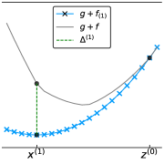
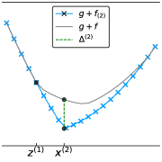
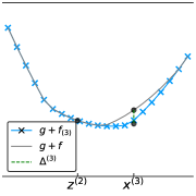
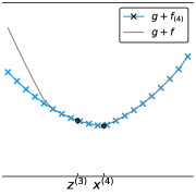
Figure 1: An illustration of L-KM (a)-(d) (left to right): blue curve marked with $\times$ denotes the $i$th function approximation $g+f_{(i)}$. In (d), note that L-KM approximation $g+f_{(4)}$ is obtained by dropping the leftmost constraint in $g+f_{(3)}$ (in (c)), unlike OSM.

L-KM and OSM differ only in the set of vertices $\mathcal{V}^{(i)}$ considered at each step: L-KM keeps only those vectors $w\in\mathcal{V}^{(i-1)}$ that maximize $w^{\top}x^{(i)}$, whereas OSM keeps every vector in $\mathcal{V}^{(i-1)}$.

We state some properties of L-KM here with proofs in Appendix C. We will revisit many of these properties later via the lens of duality.

The sets $\mathcal{V}^{(i)}$ in L-KM are affinely independent, which shows the size of the subproblems is bounded.

Theorem 3.1.

For all $i\geq 0$, vectors in $\mathcal{V}^{(i)}$ are affinely independent. Moreover, $|\mathcal{V}^{(i)}|\leq n+1$.

L-KM may discard pieces of the lower approximation $f_{(i)}$ at each iteration. However, it does so without any adverse affect on the solution to the current subproblem:

Lemma 3.2.

The convex subproblem (in Step 3 of algorithm L-KM) has the same solution and optimal value over the new active set $\mathcal{A}^{(i)}$ as over the memory $\mathcal{V}^{(i-1)}$:

$$x^{(i)}=\operatorname*{argmin}g(x)+\max\{w^{\top}x:w\in\mathcal{V}^{(i-1)}\}=\operatorname*{argmin}g(x)+\max\{w^{\top}x:w\in\mathcal{A}^{(i)}\}.$$

Lemma 3.2 shows that L-KM remembers the important information about the solution, i.e. only the tight subgradients, at each iteration. Note that at the $i$th iteration, the solution $x^{(i)}$ is unique by the strong convexity of $g$, and thus we can improve the lower bound $d^{(i)}$ since new information (i.e. $v^{(i)}$) is added:

Corollary 3.3.

The sequence {$d^{(i)}$} constructed by L-KM form strictly increasing lower bounds on the value of ($P$): $d^{(1)}<d^{(2)}<\cdots\leq p^{\star}\overset{\Delta}{=}\min_{x\mathop{\in}\mathbb{R}^{n}}f(x)+g(x)$.

Remark 3.4.

It is easy to see that the sequence $\{p^{(i)}\}$ constructed by L-KM form upper bounds of $p^{\star}$, hence by Corollary 3.3, $\{p^{(i)}-d^{(i)}\}$ form valid optimality gaps for L-KM.

Corollary 3.5.

L-KM does not stall: for any iterations $i_{1}\neq i_{2}$, we solve subproblems over a distinct set of vertices $\mathcal{V}^{(i_{1})}\neq\mathcal{V}^{(i_{2})}$.

We can strengthen Corollary 3.5 and show L-KM in fact converges to the exact solution in finite iterations:

Theorem 3.6.

L-KM (Algorithm 1) terminates after finitely many iterations. Moreover, for any given $\epsilon\geq 0$, suppose L-KM terminates when $i=i_{\epsilon}$, then $p^{\star}+\epsilon\geq p^{(i_{\epsilon})}\geq p^{\star}$ and $p^{\star}\geq d^{(i_{\epsilon})}\geq p^{\star}-\epsilon$. In particular, when we choose $\epsilon=0$, we have $p^{(i_{0})}=p^{\star}=d^{(i_{\epsilon})}$, and $x^{(i_{\epsilon})}$ is the unique optimal solution to ($P$).

In this section, we have shown that L-KM solves a series of limited memory convex subproblems with no more than $n+1$ linear constraints, and produces strictly increasing lower bounds that converge to the optimal value.

4 Duality

L-KM solves a series of subproblems parametrized by the sets $\mathcal{V}\subseteq\mathop{\textup{vert}}(B(F))$:

(P(V)) $$\begin{array}[]{ll}\mathop{\textup{minimize}}&g(x)+t\\ \mathop{\textup{subject to}}&t\geq v^{\top}x,\quad v\in\mathcal{V}\end{array}$$

Notice that when $\mathcal{V}=\mathop{\textup{vert}}(B(F))$, we recover ($P$). We now analyze these subproblems via duality. The Lagrangian of this problem with dual variables $\lambda_{v}$ for $v\in\mathcal{V}$ is,

$$\mathcal{L}(x,t,\lambda)=g(x)+t+\sum_{v\in\mathcal{V}}\lambda_{v}(v^{\top}x-t).$$

The pair $((x,t),\lambda)$ are primal-dual optimal for this problem iff they satisfy the KKT conditions [5]:

• Optimality.

  $$0\in\partial_{x}\mathcal{L}(x,t,\lambda)\implies\sum_{v\in\mathcal{V}}\lambda_{v}v\in-\partial g(x),\qquad 0=\frac{d}{dt}\mathcal{L}(x,t,\lambda)\implies\sum_{v\in\mathcal{V}}\lambda_{v}=1.\\$$

• Primal feasibility. $t\geq v^{\top}x$ for each $v\in\mathcal{V}$.

• Dual feasibility. $\lambda_{v}\geq 0$ for each $v\in\mathcal{V}$.

• Complementary slackness. $\lambda_{v}(v^{\top}x-t)=0$ for each $v\in\mathcal{V}$.

The requirement that $\lambda$ lie in the simplex emerges naturally from the optimality conditions, and reduces the Lagrangian to $\mathcal{L}(x,\lambda)=g(x)+(\sum_{v\in\mathcal{V}}\lambda_{v}v)^{\top}x$. One can introduce the variable $w=\sum_{v\in\mathcal{V}}\lambda_{v}v\in\operatorname*{conv}(\mathcal{V})$, which is dual feasible so long as $w\in\operatorname*{conv}(\mathcal{V})$. We can rewrite the Lagrangian in terms of $x$ and $w\in\operatorname*{conv}(\mathcal{V})$ as $L(x,w)=g(x)+w^{\top}x.$ Minimizing $L(x,w)$ over $x$, we obtain the dual problem

(D(V)) $$\begin{array}[]{ll}\mathop{\textup{maximize}}&-g^{*}(-w)\\ \mathop{\textup{subject to}}&w\in\operatorname*{conv}(\mathcal{V}).\end{array}$$

Note ($D$) is the same as (D(V)) if $\mathcal{V}=\mathrm{vert}(B(F))$ and $h(w)=-g^{*}(-w)$, the Fenchel conjugate of $g$. Notice that $g^{*}$ is smooth if $g$ is strongly convex (Lemma A.2 in Appendix A.2).

Theorem 4.1 (Strong Duality).

The primal problem (P(V)) and the dual problem (D(V)) have the same finite optimal value.

By analyzing the KKT conditions, we obtain the following result, which we will used later in the design of our algorithms.

Lemma 4.2.

Suppose $(x,\lambda)$ solve ((P(V)), (D(V))) and $t=\max_{v\in\mathcal{V}}v^{\top}x$. By complementary slackness,

$$\lambda_{v}>0 \implies v^{\top}x=t,$$

$$\text{and in particular,}~{}~{}\{v:\lambda_{v}>0\} \subseteq \{v:v^{\top}x=t\}.$$

Notice $\{v:v^{\top}x=t\}$ is the active set of L-KM. We will see $\{v:\lambda_{v}>0\}$ is the (minimal) active set of the dual method L-FCFW. (If strict complementary slackness holds, these sets are the same.)

The first KKT condition shows how to move between primal and dual optimal variables.

Theorem 4.3.

If $g:\mathbb{R}^{n}\to\mathbb{R}$ is strongly convex and $w^{\star}$ solves (D(V)), then

(5) $$x^{\star}=(\partial g)^{-1}(-w^{\star})=\nabla g^{*}(-w^{\star})$$

solves (P(V)). If in addition $g$ is smooth and $x^{\star}$ solves (P(V)), then $w^{\star}=\nabla g(x^{\star})$ solves (D(V)).

Proof 4.4.

Check the optimality conditions to prove the result. By definition, $x^{\star}$ satisfies the first optimality condition. To check complementary slackness, we rewrite the condition as

$$\lambda_{v}(v^{\top}x-t)=0\quad\forall v\in\mathcal{V}\iff\left(\sum_{v\in\mathcal{V}}\lambda_{v}v\right)^{\top}x=t\iff w^{\top}x=\max_{v\in\mathcal{V}}v^{\top}x.$$

Notice $(w^{\star})^{\top}(\nabla g^{*}(-w^{\star}))=\max_{v\in\mathcal{V}}v^{\top}(\nabla g^{*}(-w^{\star}))$ by optimality of $w^{\star}$, since $v-w^{\star}$ is a feasible direction for any $v\in\mathcal{V}$, proving $x^{\star}=\nabla g^{*}(-w^{\star})$ solves (P(V)).

That the primal optimal variable yields a dual optimal variable via $w^{\star}=\nabla g(x^{\star})$ follows from a similar argument together with ideas from the proof of strong duality in Appendix D.

5 Solving the dual problem

Let’s return to the dual problem ($D$): maximize a smooth concave function $h(w)=-g^{*}(-w)$ over the polytope $B(F)\subseteq\mathbb{R}^{n}$. Linear optimization over this polytope is easy; hence a natural strategy is to use the Frank-Wolfe method or one of its variants [15]. However, since the cost of each linear minimization is not negligible, we will adopt a Frank-Wolfe variant that makes considerable progress at each iteration by solving a subproblem of moderate complexity: Limited Memory fully corrective Frank-Wolfe (L-FCFW, Algorithm 2), which at every iteration exactly minimizes the function $-g^{*}(-w)$ over the the convex hull of the current subset of vertices $\mathcal{V}^{(i)}$. Here we overload notation intentionally: when $g$ is smooth and strongly convex, we will see that we can choose the set of vertices $\mathcal{V}^{(i)}$ in L-FCFW (Algorithm 2) so that the algorithm matches either L-KM or OSM depending on the choice of $\mathcal{B}^{(i)}$ (8 of L-FCFW). For details of the duality between L-KM and L-FCFW see Section 6.

Algorithm 2 L-FCFW: Limited Memory Fully Corrective Frank Wolfe for ($D$)

1:smooth concave function $h:\mathbb{R}^{n}\rightarrow\mathbb{R}$, submodular function $F:2^{n}\rightarrow\mathbb{R}$, tolerance $\epsilon\geq 0$

2:$\epsilon$-suboptimal solution $w^{\sharp}$ to ($D$)

3:initialize: set $\emptyset\subset\mathcal{V}^{(0)}\subseteq\mathrm{vert}(B(F))$

4:for $i=1,2,\ldots$ do

5:    Convex subproblem. Solve

$$w^{(i)}=\operatorname*{argmax}\{h(w):w\in\operatorname*{conv}(\mathcal{V}^{(i-1)})\}.$$

For each $v\in\mathcal{V}^{(i)}$, define $\lambda_{v}\geq 0$ so that $w^{(i)}=\sum_{v\in\mathcal{V}^{(i)}}\lambda_{v}v$ and $\sum_{v\in\mathcal{V}^{(i)}}\lambda_{v}=1$.

6:    Submodular subproblem. Compute gradient $x^{(i)}=\nabla h(w^{(i)})$ and solve

$$v^{(i)}=\operatorname*{argmax}\{w^{\top}x^{(i)}:w\in B(F)\}.$$

7:    Stopping condition. Break if duality gap $p^{(i)}-d^{(i)}\leq\epsilon$, where

$$p^{(i)}=(v^{(i)})^{\top}x^{(i)},\qquad d^{(i)}=(w^{(i)})^{\top}x^{(i)}.$$

8:    Update memory. Identify a supserset of active vertices $\mathcal{B}^{(i)}$ and update memory $\mathcal{V}^{(i)}$:

$$\mathcal{B}^{(i)}\supseteq\{w\in\mathcal{V}^{(i-1)}:\lambda_{w}>0\}\qquad\mathcal{V}^{(i)}=\mathcal{B}^{(i)}\cup\{v^{(i)}\}.$$

9:return $w^{(i)}$

Limited memory.

In L-FCFW, we may choose any active set $\mathcal{B}^{(i)}\supseteq\{w\in\mathcal{V}^{(i-1)}:\lambda_{w}>0\}$. When $\mathcal{B}^{(i)}=\mathcal{V}^{(i-1)}$, we call the algorithm (vanilla) FCFW. When $\mathcal{B}^{(i)}$ is chosen to be small, we call the algorithm Limited Memory FCFW (L-FCFW). Standard FCFW increases the size of the active set at each iteration, whereas the most limited memory variant of L-FCFW uses only those vertices needed to represent the iterate $w^{(i)}$.

Moreover, recall Carathéodory’s theorem (see e.g. [23]): for any set of vectors $\mathcal{V}$, if $x\in\operatorname*{conv}(\mathcal{V})\subseteq\mathbb{R}^{n}$, then there exists a subset $A\subseteq\mathcal{V}$ with $|A|\leq n+1$ such that $x\in\operatorname*{conv}(A)$. Hence we see we can choose $\mathcal{B}^{(i)}$ to contain at most $n+1$ vertices at each iteration (hence $n+2$ in $\mathcal{V}^{(i)}$), or even fewer if the iterate lies on a low-dimensional face of $B(F)$. (The size of $\mathcal{B}^{(i)}$ may depend on the solver used for (D(V)); to reduce the size of $\mathcal{B}^{(i)}$, we can minimize a random linear objective over the optimal set of (D(V)) as in [22].)

Linear convergence.

Lacoste-Julien and Jaggi [15] show that FCFW converges linearly to an $\epsilon$-suboptimal solution when $g$ is smooth and strongly convex so long as the active set $\mathcal{B}^{(i)}$ and iterate $x^{(i)}$ satisfy three conditions they call approximate correction($\epsilon$):

1. Better than FW. $h(y^{(i)})\leq\min_{\lambda\mathop{\in}[0,1]}h((1-\lambda)w^{(i-1)}+\lambda v^{(i-1)}))$.

2. Small away-step gap. $\max\{(w^{(i)}-v)^{\top}x^{(i)}:v\mathop{\in}\mathcal{V}(w^{(i)})\}\leq\epsilon$, where $\mathcal{V}(w^{(i)})=\{v\in\mathcal{V}^{(i-1)}:\lambda_{v}>0\}$.

3. Representation. $x^{(i)}\in\operatorname*{conv}(\mathcal{B}^{(i)})$.

By construction, iterates of L-FCFW always satisfy these conditions with $\epsilon=0$:

1. Better than FW. For any $\lambda\in[0,1]$, $w=(1-\lambda)w^{(i-1)}+\lambda v^{(i-1)}$ is feasible.

2. Zero away-step gap. For each $v\mathop{\in}\mathcal{V}^{(i)}$, if $w^{(i)}=v$, then clearly $(w^{(i)}-v)^{\top}(x^{(i)})=0$. otherwise (if $w^{(i)}\neq v$) $v-w^{(i)}$ is a feasible direction, and so by optimality of $w^{(i)}$ $(w^{(i)}-v)^{\top}(x^{(i)})\leq 0$.

3. Representation. We have $w^{(i)}\in\operatorname*{conv}(\mathcal{B}^{(i)})$ by construction of $\mathcal{B}^{(i)}$.

Hence we have proved Theorem 5.1:

Theorem 5.1.

Suppose $g$ is $\alpha$-smooth and $\beta$-strongly convex. Let $M$ be the diameter of $B(F)$ and $\delta$ be the pyramidal width of $P$, then the lower bounds $d^{(i)}$ in L-FCFW (Algorithm 2) converges linearly at the rate of $1-\rho$, i.e. $p^{\star}-d^{(i+1)}\leq(1-\rho)(p^{\star}-d^{(i)})$, where $\rho\overset{\Delta}{=}\frac{\beta}{4\alpha}(\frac{\delta}{M})^{2}$.

Primal-from-dual algorithm.

Recall that dual iterates yield primal iterates via Theorem 4.3. Hence the gradients $x^{(i)}=-\nabla g^{*}(-w^{(i)})$ computed by L-FCFW converge linearly to the solution $x^{\star}$ of ($P$). However, it is difficult to run L-FCFW directly to solve ($D$) given only access to $g$, since in that case computing $g^{*}$ and its gradient requires solving another optimization problem; moreover, we will see below that L-KM computes the same iterates. See Appendix E for more discussion.

6 L-KM (and OSM) converge linearly

L-KM (Algorithm 1) and L-FCFW (Algorithm 2) are dual algorithms in the following strong sense:

Theorem 6.1.

Suppose $g$ is $\alpha$-smooth and $\beta$-strongly convex. In L-FCFW (Algorithm 2), suppose we choose $\mathcal{B}^{(i)}=\mathcal{A}^{(i)}=\{v\in\mathcal{V}^{(i-1)}:v^{\top}x^{(i)}={w^{(i)}}^{\top}x^{(i)}\}$. Then

1. The primal iterates $x^{(i)}$ of L-KM and L-FCFW match.

2. The sets $\mathcal{V}^{(i)}$ used at each iteration of L-KM and L-FCFW match.

3. The upper and lower bounds $p^{(i)}$ and $d^{(i)}$ of L-KM and L-FCFW match.

Corollary 6.2.

The active sets of L-FCFW can be chosen to satisfy $|\mathcal{B}^{(i)}|\leq n+1$.

Theorem 6.3.

Suppose $g$ is $\alpha$-strongly convex and let $M$ be the diameter of $B(F)$, the duality gap $p^{(i)}-d^{(i)}$ in L-KM (Algorithm 1) converges linearly: $p^{(i)}-d^{(i)}\leq(p^{\star}-d^{(i)})+M^{2}/(2\beta)$ when $(p^{\star}-d^{(i)})\geq M^{2}/(2\beta)$ and $p^{(i)}-d^{(i)}\leq M\sqrt{2(p^{\star}-d^{(i)})/\beta}$ otherwise. Note that $p^{\star}-d^{(i)}$ converges linearly by Theorem 5.1.

When $g$ is smooth and strongly convex, OSM and vanilla FCFW are dual algorithms in the same sense when we choose $\mathcal{B}^{(i)}=\mathcal{V}^{(i-1)}$. For details of the duality between OSM and L-FCFW see Appendix G. Hence we have a similar convergence result for OSM:

Theorem 6.4.

Suppose $g$ is $\alpha$-strongly convex and let $M$ be the diameter of $B(F)$, the duality gap $p^{(i)}-d^{(i)}$ in OSM converges linearly: $p^{(i)}-d^{(i)}\leq(p^{\star}-d^{(i)})+M^{2}/(2\beta)$ when $(p^{\star}-d^{(i)})\geq M^{2}/(2\beta)$ and $p^{(i)}-d^{(i)}\leq M\sqrt{2(p^{\star}-d^{(i)})/\beta}$ otherwise.

Remark 6.5.

Note that $p^{\star}-d^{(i)}$ converges linearly by Theorem 5.1, Theorem 6.3 and Theorem 6.3 imply L-KM and OSM converge linearly when $g$ is smooth and strongly convex.

Moreover, this connection generates a new way to prune the active set of L-KM even further using a primal dual solver: we may use any active set $\mathcal{B}^{(i)}\supseteq\{w\in\mathcal{V}^{(i-1)}:\lambda_{w}>0\}$, where $\lambda\in\mathbb{R}^{|\mathcal{V}^{(i-1)}|}$ is a dual optimal solution to (P(V)). When strict complementary slackness fails, we can have $\mathcal{B}^{(i)}\subset\mathcal{A}^{(i)}$.

7 Experiments and Conclusion

We present in this section a computational study: we minimize non-separable composite functions $g+f$ where $g(x)=x^{\top}(A+n\mathbf{I}_{n})x+b^{\top}x$ for $x\in\mathbb{R}^{n}$, and $f$ is the Lovász extension of the submodular function $F(A)\mathop{=}\frac{|A|(2n-|A|+1)}{2}$ for $A\subseteq[n]$. To construct $g(\cdot)$, entries of $A\in M_{n}$ and $b\in\mathbb{R}^{n}$ were randomly sampled from $U[-1,1]^{n\times n}$, and $U[0,n]^{n}$ respectively. $\mathbf{I}_{n}$ is an $n\times n$ identity matrix.

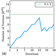
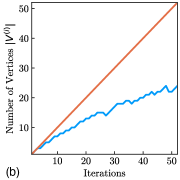
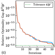
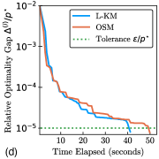
Figure 2: Dimension $n=10$ in (a), $n=100$ in (b), (c) and (d). The methods converged in (a), (b), (c) and (d).

We remark that L-KM converges so quickly that the bound on the size of the active set is less important, in practice, than the fact that the active set need not grow at every iteration.

Primal convergence: We first solve a toy problem Primal convergence: We first solve a toy problem for $n=10$ and show that the number of constraints does not exceed $n+1$. Note that the number of constraints might oscillate before it reaches $n+1$ (Fig. 2(a)). We next compare the memory used in each iteration (Fig. 2(b)), the optimality gap per iteration (Fig. 2(c)), and the running time (Fig. 2(d)) of L-KM and OSM by solving the problem for $n=100$ up to accuracy of $10^{-5}$ of the optimal value. Note that L-KM uses much less memory compared to OSM, converges at almost the same rate in iterations, and its running time per iteration improves as the iteration count increases.

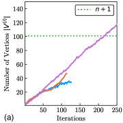
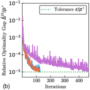
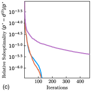
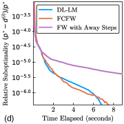
Figure 3: L-FCFW and FCFW converged in all plots, FW with away steps has converged in (b), (c) and (d).

Dual convergence: We compare the convergence of L-FCFW, FCFW and Frank-Wolfe with away steps for the dual problem $\max_{w\mathop{\in}B(F)}-(-w-b)^{\top}(A+n\mathbf{I}_{n})^{-1}(-w-b)$ for $n=100$ up to relative accuracy of $10^{-5}$. L-FCFW maintains smaller sized subproblems (Figure (3)(a)), and it converges faster than FCFW as the number of iteration increases (Figure (3)(d)). Their provable duality gap converges linearly in the number of iterations. Moreover, as shown in Figures (3)(b) and (c), L-FCFW and FCFW return better approximate solutions than Frank-Wolfe with away steps under the same optimality gap tolerance.

Conclusion This paper defines a new limited memory version of Kelley’s method adapted to composite convex and submodular objectives, and establishes the first convergence rate for such a method, solving the open problem proposed in [2, 3]. We show bounds on the memory requirements and convergence rate, and demonstrate compelling performance in practice.

Acknowledgments

This work was supported in part by DARPA Award FA8750-17-2-0101. A part of this work was done while the first author was at the Department of Mathematical Sciences, Tsinghua University and while the second author was visiting the Simons Institute, UC Berkeley. The authors would also like to thank Sebastian Pokutta for invaluable discussions on the Frank-Wolfe algorithm and its variants.

Appendix A Additional Background

A.1 Additional Examples

We list some examples of popular submodular functions in Table 1.

Problem	Submodular function, $S\subseteq E$ (unless specified)
n experts (simplex), $E=\{1,\ldots,n\}$	$f(S)=1$
k out of n experts (k-simplex), $E=\{1,\ldots,n\}$	$f(S)=\min\{|S|,k\}$
Permutations over $E=\{1,\ldots,n\}$	$f(S)=\sum_{s=1}^{|S|}(n+1-s)$
k-truncated permutations over $E=\{1,\ldots,n\}$	$f(S)=(n-k)|S|$ for $|S|\leq k$, $f(S)=k(n-k)+\sum_{s=k+1}^{|S|}(n+1-s)$ if $|S|\geq k$
Spanning trees on $G=(V,E)$	$f(S)=|V(S)|-\kappa(S)$, $\kappa(S)$ is the number of connected components of $S$
Matroids over ground set $E$: $M=(E,\mathcal{(I)}),\mathcal{(I)}\subseteq 2^{E}$	$f(S)=r_{M}(S)$, the rank function of the matroid
Coverage of T: given $T_{1},\ldots,T_{n}\subseteq T$	$f(S)=|\bigcup_{i\in S}T_{i}|$, $E=\{1,\ldots,n\}$
Cut functions on a directed graph $D=(V,E)$, $c:E\rightarrow\mathbb{R}_{+}$	$f(S)=c(\delta^{out}(S))$, $S\subseteq V$
Flows into a sink vertex $t$, given a directed graph $D=(V,E)$ and costs $c:E\rightarrow\mathbb{R}_{+}$	$f(S)=$ max flow from $S\subseteq V\setminus\{t\}$ into $t$
Maximal elements in $E$, $h:E\rightarrow\mathbb{R}$	$f(S)=\max_{e\in S}h(e)$, $f(\emptyset)=\min_{e\in E}h(e)$
Entropy $H$ of random variables $X_{1},\ldots,X_{n}$	$f(S)=H(\bigcup_{i\in S}X_{i})$, $E=\{1,\ldots,n\}$

Table 1: Problems and the submodular functions (on ground set of elements $E$) that give rise to them.

A.2 Strong Convexity and Smoothness

We say a function $g:\mathbb{R}^{n}\rightarrow\mathbb{R}$ is $\alpha$-strongly convex if $g(x)-\alpha/2\|x\|^{2}$ is convex, where $\alpha>0$. It is easy to see that the sum of a stronly convex function and a piecewise linear function is still strongly convex, and we have

Lemma A.1.

When $g:\mathbb{R}^{n}\rightarrow\mathbb{R}$ is a strongly convex function, then

(P(V)) $$\begin{array}[]{ll}\mathop{\textup{minimize}}&g(x)+\max_{w\mathop{\in}\mathop{\mathrm{conv}(\mathcal{V})}}w^{\top}x\\ \end{array}$$

has a unique optimal solution $x^{\star}$ for all $\mathcal{V}\subseteq\mathbb{R}^{n}$.

On the other hand, we say a function $g:\mathbb{R}^{n}\rightarrow\mathbb{R}$ is $\beta$-smooth if there exists $\beta>0$ such that $g(x)-\beta/2\|x\|^{2}$ is concave. We have[21]:

Lemma A.2.

When a function $g$ is $\alpha$-strongly convex, its Fenchel conjugate $g^{*}$ is $\frac{1}{\alpha}$- smooth.

Lemma A.3.

When a function $g$ is $\beta$-smooth, its Fenchel conjugate $g^{*}$ is $\frac{1}{\beta}$-strongly convex.

Appendix B The Original Simplicial Method (Section 3)

We present the Original Simplicial Method (OSM) in Algorithm 3.

Algorithm 3 OSM: The Original Simplicial Method for ($P$)

1:strongly convex function $g:\mathbb{R}^{n}\rightarrow\mathbb{R}$, submodular function $F:2^{n}\rightarrow\mathbb{R}$, tolerance $\epsilon>0$

2:$\epsilon$-suboptimal solution $x^{\sharp}$

3:initialize: choose $x^{(0)}\in\mathbb{R}^{n}$, set $\mathcal{V}^{(0)}=\emptyset$

4:for i=1,2,… do

5:    Convex subproblem. Define approximation $f_{(i)}(x)=\max\{w^{\top}x:w\mathop{\in}\mathcal{V}^{(i-1)}\}$ and solve

$$x^{(i)}=\operatorname*{argmin}g(x)+f_{(i)}(x).$$

6:    Submodular subproblem. Compute value and subgradient of $f$ at $x^{(i)}$

$$f(x^{(i)})=\max_{w\in B(F)}w^{\top}x^{(i)},\qquad v^{(i)}\mathop{\in}\partial f(x^{(i)})=\operatorname*{argmax}_{w\in B(F)}w^{\top}x^{(i)}.$$

7:    Stopping condition. Break if duality gap $p^{(i)}-d^{(i)}\leq\epsilon$, where

$$p^{(i)}=g(x^{(i)})+f(x^{(i)}),\qquad d^{(i)}=g(x^{(i)})+f_{(i)}(x^{(i)}).$$

8:    Update memory. Update memory $\mathcal{V}^{(i)}$:

$$\mathcal{V}^{(i)}=\mathcal{V}^{(i-1)}\cup\{v^{(i)}\}.$$

9:return $x^{(i)}$

Appendix C Limited Memory Kelley’s Method (Section 3)

In this section, we provide proofs of some of the results in Section 3.

Proof of Theorem 3.1.

Proof C.1.

We prove this by induction. The claim is true for $i=0$ since $\mathcal{V}^{(0)}$ has only one element. Suppose that the claim is true for $i<i_{0}$. When $\Delta>\epsilon$, we have ${v^{(i_{0})}}^{\top}x^{(i_{0})}=f(x^{(i_{0})})>f_{(i_{0})}(x^{(i_{0})})$. From $\mathcal{A}^{(i_{0})}\subseteq\{w\in\mathbb{R}^{n}\mid w^{\top}x^{(i_{0})}=f_{(i_{0})}(x^{(i_{0})})\}$ we have $v^{(i_{0})}\notin\mathop{\mathrm{affine}}(\mathcal{A}^{(i_{0})})$. Otherwise when $\Delta^{(i)}\leq\epsilon$, the algorithm terminates in the $i_{0}$th iteration.

Since vectors in $\mathcal{V}^{(i)}$ are affinely independent, we have $|\mathcal{V}^{(i)}|\leq n+1$ for all $i$ since $\mathcal{V}^{(i)}\subseteq\mathbb{R}^{n}$.

Before proving Lemma 3.2, we first present a lemma that is used in the proof of Lemma 3.2:

Lemma C.2.

Given a submodular function $F:2^{V}\to\mathbb{R}$, let $\mathcal{W}\subseteq\mathop{\mathrm{vert}}(B(F))$ be a subset of the vertices of its base polytope. For the piecewise linear function

$$\tilde{f}(x)=\max_{w\mathop{\in}\mathop{\mathrm{conv}}(\mathcal{W})}w^{\top}x,$$

let $\mathcal{A}(x)\overset{\Delta}{=}\{w^{\star}\in\mathcal{W}\mid{w^{\star}}^{\top}x=\tilde{f}(x)\}$ be the points in $\mathcal{W}$ that are active at $x$. Then given any $\bar{x}\in\mathbb{R}^{n}$, there exists $\epsilon>0$ such that

$$\tilde{f}(x)=\max_{w^{\star}\mathop{\in}\mathop{\mathrm{conv}}(\mathcal{A}(\bar{x}))}{w^{\star}}^{\top}x$$

for all $x\in\mathcal{B}(\bar{x},\ \epsilon)$.

Proof C.3.

Since $\mathcal{W}$ is finite, we have $\tilde{f}(\bar{x})\geq\max_{\tilde{w}\in\mathcal{W}\setminus\mathcal{A}(\bar{x})}\tilde{w}^{\top}\bar{x}+\epsilon$, where $\epsilon>0$. Let $L=\max_{w\in\mathcal{W}}\|w\|$, then for all $x\in\mathcal{B}(\bar{x},\ \epsilon/(3L))$, $w^{\star}\in\mathcal{A}(\bar{x})$ and $\tilde{w}\in\mathcal{W}\setminus\mathcal{A}(\bar{x})$, we have

(6) $$\begin{split}{w^{\star}}^{\top}x-\tilde{w}^{\top}x&=({w^{\star}}-\tilde{w})^{\top}\bar{x}+{w^{\star}}^{\top}(x-\bar{x})+\tilde{w}^{\top}(\bar{x}-x)\\ &\geq\epsilon-L\frac{\epsilon}{3L}-L\frac{\epsilon}{3L}\\ &=\frac{\epsilon}{3}.\end{split}$$

Hence $\tilde{f}(x)>\tilde{w}^{\top}x$ for all $x\in\mathcal{B}(\bar{x},\ \epsilon/(3L))$ and $\tilde{w}\in\mathcal{W}\setminus\mathcal{A}(\bar{x})$, which is equivalent to $\tilde{f}(x)=\max_{w^{\star}\mathop{\in}\mathop{\mathrm{conv}}(\mathcal{A}(\bar{x}))}{w^{\star}}^{\top}x$ for all $x\in\mathcal{B}(\bar{x},\ \epsilon/(3L))$.

Proof of Lemma 3.2.

Proof C.4.

Let $P_{(i)}(x)\overset{\Delta}{=}\min g(x)+\max_{w\mathop{\in}\mathop{\mathrm{conv}}(\mathcal{V}^{(i-1)})}w^{\top}x=g(x)+f_{(i)}(x)$ and $\widetilde{P}_{(i)}\overset{\Delta}{=}\min_{x\mathop{\in}\mathbb{R}^{n}}g(x)+\max_{w\mathop{\in}\mathop{\mathrm{conv}}(\mathcal{A}^{(i)})}w^{\top}x$. There exists at least one $w^{\star}\in\mathcal{V}^{(i-1)}$ such that $f_{(i)}(x^{(i)})=w^{\star T}x^{(i)}$. Therefore, $P_{(i)}(x^{(i)})=g(x^{(i)})+w^{\star T}x^{(i)}=g(x^{(i)})+\max_{w\in\mathop{\mathrm{conv}}(\mathcal{A}^{(i)})}w^{\top}x^{(i)}=\widetilde{P}_{(i)}(x^{(i)})$, where the last equality follows from the definition of $\mathcal{A}^{(i)}$. Next, if we can show local optimality of $x^{(i)}$ for $\widetilde{P}_{(i)}$, this would imply global optimality of $x^{(i)}$ for $\widetilde{P}_{(i)}$ due to convexity of $\widetilde{P}_{(i)}$, thus ${P}_{(i)}$ and $\widetilde{P}_{(i)}$ will have the same optimal value. By the definition of $\mathcal{A}^{(i)}$ and Lemma C.2, we have $f(x)=\max_{w\in\mathop{\mathrm{conv}}(\mathcal{A}(x^{(i)}))}=f_{(i)}(x^{(i)})$ in $\mathcal{B}(x^{(i)},\ \epsilon)$ for some $\epsilon>0$. Thus $P_{(i)}(x^{(i)})=g(x)+f(x)=g(x)+f_{(i)}(x)=\widetilde{P}_{(i)}(x)$ for $x\in\mathcal{B}(x^{(i)},\ \epsilon)$. Hence $x^{(i)}$ is an local optimal solution to $\widetilde{P}_{(i)}$, and the lemma is proved. By Lemma A.1, $x^{(i)}$ is the unique solution to both $P_{(i)}$ and $\widetilde{P}_{(i)}$.

Proof of Corollary 3.3.

Proof C.5.

For any $i\geq 1$, by Lemma A.1, there exists an $x^{(i)}\in\mathbb{R}^{n}$ that minimizes $g(x)+f_{(i)}(x)$. Thus we have

$$d^{(i)} =g(x^{(i)})+f_{(i)}(x^{(i)})$$

$$=g(x^{(i)})+\max_{w\in\mathop{\mathrm{conv}}(\mathcal{V}^{(i-1)})}w^{\top}x^{(i)}$$

(7) $$\geq g(x^{(i)})+\max_{w\in\mathop{\mathrm{conv}}(\mathcal{A}^{(i-1)})}w^{\top}x^{(i)} \triangleright\ \mathcal{A}^{(i-1)}\subseteq\mathcal{V}^{(i-1)}$$

$$>g(x^{(i-1)})+\max_{w\in\mathop{\mathrm{conv}}(\mathcal{A}^{(i-1)})}w^{\top}x^{(i-1)} \triangleright\ \text{optimality and uniqueness of }x^{(i-1)}$$

$$=d^{(i-1)}.$$

On the other hand, by $\mathcal{V}^{(i-1)}\subseteq\mathop{\mathrm{vert}}(B(F))$, we have

(8) $$\begin{split}d^{(i)}&=\min_{x\mathop{\in}\mathbb{R}^{n}}\{g(x)+\max_{w\in\mathop{\mathrm{conv}}(\mathcal{V}^{(i-1)})}w^{\top}x\}\\ &\leq\min_{x\mathop{\in}\mathbb{R}^{n}}\{g(x)+\max_{w\in B(F)}w^{\top}x\}\\ &=\min_{x\mathop{\in}\mathbb{R}^{n}}g(x)+f(x)\end{split}$$

for all $i\geq 0$.

Proof of Corollary 3.5.

Proof C.6.

Note that each $\mathcal{V}^{(i)}$ determines a unique $d^{(i)}$. Suppose for contradiction that there exists $i_{1}\neq i_{2}$ but $\mathcal{V}^{(i_{1})}=\mathcal{V}^{(i_{2})}$, then we will have $d^{(i_{1})}=d^{(i_{2})}$, which contradicts the fact that {$d^{(i)}$} strictly increases.

Proof of Theorem 3.6

Proof C.7.

Since $\mathop{\mathrm{vert}}(B(F))$ has finitely many vertices, there are only finitely many choices of $\mathcal{V}^{(i)}\subseteq\mathop{\mathrm{vert}}(B(F))$. Thus by Corollary 3.5, Algorithm 1 terminates within finitely many steps.

Suppose for contradiction that when the algorithm terminates at $i=i_{0}$, $p^{(i_{0})}-d^{(i_{0})}>\epsilon\geq 0$. Let $\mathcal{A}^{(i_{0})}\overset{\Delta}{=}\{w\in\mathcal{V}^{(i_{0}-1)}:w^{\top}{x^{(i_{0})}}\overset{\Delta}{=}f_{(i_{0})}(x^{(i_{0})})$ and $v^{(i_{0})}\in\mathcal{V}(x^{(i_{0})})$. Define $\mathcal{V}^{(i_{0})}\overset{\Delta}{=}\mathcal{A}^{(i_{0})}\cup\{v^{(i_{0})}\}$ and $f_{(i_{0}+1)}(x)=\max\{w^{\top}x:w\mathop{\in}\mathcal{V}^{(i_{0})}\}$, then let $x^{(i_{0}+1)}=\operatorname*{argmin}_{x\mathop{\in}\mathbb{R}^{n}}g(x)+f_{(i_{0}+1)}(x)$. By the proof of Corollary 3.3, we have $d^{(i_{0}+1)}=g(x^{(i_{0}+1)})+f_{(i_{0}+1)}(x^{(i_{0}+1)})>d^{i_{0}}$, so $\mathcal{V}^{(i_{0})}$ is different to any $V^{(i)}$ where $i\leq i_{0}$, and L-KM should not have terminated at $i=i_{0}$. Thus L-KM would never terminate when $p^{(i)}-d^{(i)}>\epsilon\geq 0$.

Appendix D Duality (Section 4)

To prove the strong duality between (P(V)) and (D(V)), we first verify the weak duality:

Theorem D.1 (Weak Duality).

The optimal value of primal problem (P(V)) is greater than or equal to the optimal value of the dual problem (D(V)).

Proof D.2.

We first have

(9) $$\min_{x\mathop{\in}\mathbb{R}^{n}}\{g(x)+\max_{w\mathop{\in}\mathop{\mathrm{conv}}(\mathcal{V})}w^{\top}x\}=\min_{x\mathop{\in}\mathbb{R}^{n}}\max_{w\mathop{\in}\mathop{\mathrm{conv}}(\mathcal{V})}g(x)+w^{\top}x.$$

For any given $\tilde{w}\in\mathop{\mathrm{conv}}(\mathcal{V})$, we also have

(10) $$\min_{x\mathop{\in}\mathbb{R}^{n}}\max_{w\mathop{\in}\mathop{\mathrm{conv}}(\mathcal{V})}g(x)+{\tilde{w}}^{\top}x\geq\min_{x\mathop{\in}\mathbb{R}^{n}}g(x)+{\tilde{w}}^{\top}x.$$

Thus by the definition of $g^{*}$, we can see that

(11) $$\begin{split}\min_{x\mathop{\in}\mathbb{R}^{n}}\max_{w\mathop{\in}\mathop{\mathrm{conv}}(\mathcal{V})}g(x)+w^{\top}x\mathop{\geq}&\max_{w\mathop{\in}\mathop{\mathrm{conv}}(\mathcal{V})}\min_{x\mathop{\in}\mathbb{R}^{n}}g(x)+w^{\top}x\\ \mathop{=}&\max_{w\mathop{\in}\mathop{\mathrm{conv}}(\mathcal{V})}-\max_{x\mathop{\in}\mathbb{R}^{n}}(-w)^{\top}x-g(x)\\ \mathop{=}&\max_{w\mathop{\in}\mathop{\mathrm{conv}}(\mathcal{V})}-g^{*}(-w).\end{split}$$

Combine (9) and (11), and the theorem follows.

Proof of Theorem 4.1

Proof D.3.

By Lemma A.1, we know (P(V)) has a unique solution $\bar{x}$. Since $g$ is convex, we have $\partial g(x)\neq\emptyset$. By the optimality of $\bar{x}$, we also have $0\in\partial g(\bar{x})+\partial f(\bar{x})$. Let $\bar{w}\in-\partial g(\bar{x})\cap\partial f(\bar{x})$, then

(12) $$g^{*}(-\bar{w})=(-\bar{w})^{\top}\bar{x}-g(\bar{x})$$

by Eq. 4. Note that $\bar{w}\in\partial f(\bar{x})$, we also have $f(\bar{x})={\bar{w}}^{\top}\bar{x}$ by Equation (2). Thus

(13) $$f(\bar{x})+g(\bar{x})=g^{*}({\bar{w}}),$$

$\bar{w}$ is an optimal solution to (D(V)) and we have (P(V)) and (D(V)) via weak duality.

Appendix E Primal-from-dual algorithm (Section 5)

Now consider the Primal-from-dual algorithm presented in Section 5.

Formally, assume $g$ is $\alpha$-strongly convex. Suppose we obtain $w\in B(F)$ with

$$\|w-w^{\star}\|\leq\epsilon$$

via some dual algorithm (e.g., L-FCFW). Define $x=\nabla_{w}(-g^{*}(-w))=\operatorname*{argmin}_{x}g(x)+w^{\top}x$. Since $g^{*}$ is $1/\alpha$ smooth, we have

$$\|x-x^{\star}\|\leq 1/\alpha\|w-w^{\star}\|\leq\epsilon/\alpha$$

Hence if the dual iterates converge linearly, so do the primal iterates.

The remaining difficulty is how to solve the L-FCFW subproblems. One possibility is to use the values and gradients of (a first order oracle for) $h=g^{*}$. To implement a first order oracle for $h=g^{*}$, we need only solve an unconstrained minimization problemma:

$$g^{*}(y)=\max_{x\mathop{\in}\mathbb{R}^{n}}y^{\top}x-g(x),\qquad\nabla g^{*}(y)=\operatorname*{argmax}_{x\mathop{\in}\mathbb{R}^{n}}y^{\top}x-g(x).$$

This problem is straightforward to solve since $g$ is smooth and strongly convex. However, it is not clear how solving these subproblems approximately affects the convergence of L-FCFW. Morever, we will see in the next section that L-KM achieves exactly the same sequence of iterates as the above (rather unwieldly) proposal.

Appendix F Duality between L-KM and L-FCFW (Section 6)

Lemma F.1.

Only vertices in $\mathcal{A}^{(i)}$ can have positive convex multipliers in the convex decomposition of $w^{(i)}$, i.e., if we write $w^{(i)}=\sum_{v\in\mathcal{V}^{(i-1)}}\lambda_{v}^{(i)}v$ such that $0\leq\lambda_{v}\leq 1$ for any $v\in\mathcal{V}^{(i-1)}$, then $\lambda_{v}^{(i)}=0$ for any $v\in\mathcal{V}^{(i-1)}\setminus\mathcal{A}^{(i)}$.

Proof F.2.

By the definition of $\mathcal{A}^{(i)}$, we have

$$\mathop{\mathop{\mathrm{conv}}}(\mathcal{A}^{(i)}) =\mathop{\mathop{\mathrm{conv}}}(\{v\in\mathcal{V}^{(i-1)}\mid v^{\top}x^{(i)}={w^{(i)}}^{\top}x^{(i)}\})$$

(14) $$=\mathop{\mathop{\mathrm{conv}}}(\{v\in\mathcal{V}^{(i-1)}\mid v^{\top}x^{(i)}=\max_{w\mathop{\in}\mathop{\mathop{\mathrm{conv}}}(\mathcal{V}^{(i-1)})}w^{\top}x^{(i)}\})$$

$$={\arg\max}_{w\mathop{\in}\mathop{\mathop{\mathrm{conv}}}(\mathcal{V}^{(i-1)})}w^{\top}x^{(i)}.$$

Then

$$0 =(w^{(i)}-w^{(i)})^{\top}x^{(i)}$$

(15) $$=(w^{(i)}-\sum_{v\mathop{\in}\mathcal{V}^{(i-1)}}\lambda_{v}^{(i)}v)$$

$$=\sum_{v\mathop{\in}\mathcal{V}^{(i-1)}\setminus\mathcal{A}^{i}}\lambda_{v}^{(i)}[(w^{(i)})^{\top}x^{(i)}-v^{\top}x^{(i)}]. \triangleright\ v^{\top}x^{(i)}={w^{(i)}}^{\top}x^{(i)},\ \mathop{\forall}v\in\mathcal{A}^{(i)}$$

By the definition of $\mathcal{A}^{(i)}$, we have $v^{\top}x^{(i)}-w^{(i)}x^{(i)}<0$ for any $v\in\mathcal{V}^{(i-1)}\setminus\mathcal{A}^{(i)}$. Thus $\lambda_{v}^{(i)}=0$ for any $v\in\mathcal{V}^{(i-1)}\setminus\mathcal{A}^{(i)}$.

Proof of Theorem 6.1.

Proof F.3.

We prove by induction. When $i=1$, $\mathcal{V}^{(0)}$ will naturally refer to the same set of points in L-KM and L-FCFW. By Lemma A.1, we have $x^{(1)}$ is the unique solution to $g+f_{(1)}$. Note $g^{*}$ is strongly convex given $g$ is smooth (Lemma A.3), we have $w^{(1)}$ is the unique solution to $\max_{w\mathop{\in}\mathop{\mathrm{conv}}(\mathcal{V}^{(0)})}-g^{*}(-w)$. Let $\mathcal{V}=\mathcal{V}^{(0)}$ in Theorem 4.3, we have that $x^{(1)}=-\nabla g^{*}(-w^{(1)})$ is the unique minimizer of $g+f_{(1)}$. So $x^{(1)}$ in the two algorithms match. Also note that $w^{(1)}$ solves $\max_{w\mathop{\in}\mathop{\mathrm{conv}}(\mathcal{V}^{(0)})}-g^{*}(-w)$, we have $w^{(1)}$ maximizes $w^{\top}x^{(1)}$ for all $w\in\mathop{\mathrm{conv}}(\mathcal{V}^{(i-1)})$ by the first order optimality condition, which gives ${w^{(i)}}^{\top}x^{(i)}=f_{(i)}(x^{(i)})$. Thus $\mathcal{A}^{(1)}$, $\mathcal{V}^{(1)}$ match consequently. By strong duality in Theorem 4.1, we have $d^{(1)}$ matches in the two algorithms. Note $g^{*}$ is strongly convex, which gives the uniqueness of $w^{(1)}$. By Theorem 4.3, $\nabla g(w^{(1)})$ solves the primal subproblem, so $x^{(1)}$ match in the two algorithms by the uniqueness of $x^{(1)}$.

Suppose that the theorem holds for $i=i_{0}$, in particular, the $\mathcal{V}^{(i_{0})}$ match in the two algorithms. Then for $i=i_{0}+1$, we can use the same argument as in the previous paragraph by substituting 0 with $i_{0}$ and 1 with $i_{0}+1$, and show that all the statements hold for $i=i_{0}+1$. Note that by Lemma F.1, $\mathcal{A}^{(i)}$ satisfies the condition in 8 of L-FCFW. Thus this theorem is valid.

Appendix G Duality between OSM and L-FCFW (Section 6)

Theorem G.1.

If $g$ is smooth and strongly convex and in Algorithm 2 we choose $\mathcal{B}^{(i)}=\mathcal{V}^{(i-1)}$, then

1. The primal iterates $x^{(i)}$ of Algorithm 3 and Algorithm 2 match.

2. The set $\mathcal{V}^{(i)}$ used at each iteration of Algorithm 3 and Algorithm 2 match.

3. The upper and lower bounds $p^{(i)}$ and $d^{(i)}$ of Algorithm 3 and Algorithm 2 match.

The proof of Theorem G.1 is similar to the proof of Theorem 6.1.

Appendix H Definition of Diameter and Pyramid Width

Diameter. The diameter of a set $\mathcal{P}\subseteq\mathbb{R}^{n}$ is defined as

(16) $$\mathop{\mathrm{Diam}}(\mathcal{P})\overset{\Delta}{=}\max_{v,\ w\mathop{\in}\mathcal{P}}\|v-w\|_{2}.$$

Directional Width. Given a direction $x\in\mathbb{R}^{n}$, the directional width of a set $\mathcal{P}\subseteq\mathbb{R}^{n}$ with respect to $x$ is defined as

(17) $$\mathop{\mathrm{dirW}}(\mathcal{P},\ x)\overset{\Delta}{=}\max_{v,\ w\mathop{\in}\mathcal{P}}{(v-w)}^{\top}\frac{x}{\|x\|_{2}}.$$

Pyramid directional width and pyramid width are defined by Lacoste-Julien and Jaggi in [15] for a finite sets of vectors $\mathcal{V}\subseteq\mathbb{R}^{n}$. Here we extend the definition of pyramid width to a polytope $\mathcal{P}=\mathop{\mathrm{conv}}(V)$, and it should be easy to see that the two definitions are essentially the same.

Pyramid Directional Width. Let $\mathcal{V}\subseteq\mathbb{R}^{n}$ be a finite set of vectors in $\mathbb{R}^{n}$. The pyramid directional width of $\mathcal{V}$ with respect to a direction $x$ and a base point $w\in\mathop{\mathrm{conv}}(\mathcal{V})$ is defined as

(18) $$\mathop{\mathrm{PdirW}}(\mathcal{V},\ x,\ w)\overset{\Delta}{=}\min_{A\mathop{\in}\mathcal{A}(w)}\mathop{\mathrm{dirW}}(A\cup\{\mathop{v}(\mathcal{V},\ x)\},\ x),$$

where $\mathcal{A}(w)\overset{\Delta}{=}\{A\subseteq\mathcal{V}\mid\text{the convex multipliers are non-zero for all}\ v\in A\ \text{in the decomposition of}\ w\}$ and $\mathop{v}(\mathcal{V},\ x)$ is a vector in $\arg\max_{v\in\mathcal{V}}v^{\top}x$. The pyramid directional width got its name because the set $A\cup\{\mathop{v}(\mathcal{V},\ x)\}$ has the shape of a pyramid with $A$ being the base and $v(\mathcal{V},\ x)$ being the summit.

Pyramid Width. The pyramid width of $\mathcal{P}$ is defined as

(19) $$\mathop{\mathrm{PWidth}}(\mathcal{P})\overset{\Delta}{=}\min_{\mathcal{K}\mathop{\in}\mathop{\mathrm{face}(\mathcal{P})}}\min_{x\mathop{\in}\mathop{\mathrm{cone}}(\mathcal{K}-w)\setminus\{0\},\ w\in{\mathcal{K}}}\mathop{\mathrm{PdirW}}(\mathcal{K}\cap\mathop{\mathrm{vert}(\mathcal{P})},\ x,\ w),$$

where $\mathop{\mathrm{face}(\mathcal{P})}$ stands for the faces of $\mathcal{P}$ and $\mathop{\mathrm{cone}}(\mathcal{K}-w)$ is equivalent to the set of vectors pointing inwards $\mathcal{K}$.

References

- [1] J. Audibert, S. Bubeck, and G. Lugosi. Regret in online combinatorial optimization. Mathematics of Operations Research, 39(1):31–45, 2013.
- [2] Francis Bach. Duality between subgradient and conditional gradient methods. SIAM Journal on Optimization, 25(1):115–129, 2015.
- [3] Francis Bach et al. Learning with submodular functions: A convex optimization perspective. Foundations and Trends® in Machine Learning, 6(2-3):145–373, 2013.
- [4] Francis R Bach. Structured sparsity-inducing norms through submodular functions. In Advances in Neural Information Processing Systems, pages 118–126, 2010.
- [5] S. Boyd and L. Vandenberghe. Convex optimization. Cambridge University Press, 2009.
- [6] E Ward Cheney and Allen A Goldstein. Newton’s method for convex programming and Tchebycheff approximation. Numerische Mathematik, 1(1):253–268, 1959.
- [7] Josip Djolonga and Andreas Krause. From MAP to marginals: Variational inference in bayesian submodular models. In Advances in Neural Information Processing Systems, pages 244–252, 2014.
- [8] Yoel Drori and Marc Teboulle. An optimal variant of Kelley’s cutting-plane method. Mathematical Programming, 160(1-2):321–351, 2016.
- [9] Marguerite Frank and Philip Wolfe. An algorithm for quadratic programming. Naval Research Logistics Quarterly, 3(1-2):95–110, 1956.
- [10] D. Hearn, S. Lawphongpanich, and J. Ventura. Restricted simplicial decomposition: Computation and extensions. Mathematical Programming Study, 31:99–118, 1987.
- [11] James E Kelley, Jr. The cutting-plane method for solving convex programs. Journal of the Society for Industrial and Applied Mathematics, 8(4):703–712, 1960.
- [12] Krzysztof C Kiwiel. Proximal level bundle methods for convex nondifferentiable optimization, saddle-point problems and variational inequalities. Mathematical Programming, 69(1-3):89–109, 1995.
- [13] W. M. Koolen, M. K. Warmuth, and J. Kivinen. Hedging structured concepts. COLT, 2010.
- [14] Walid Krichene, Syrine Krichene, and Alexandre Bayen. Convergence of mirror descent dynamics in the routing game. In European Control Conference (ECC), pages 569–574. IEEE, 2015.
- [15] Simon Lacoste-Julien and Martin Jaggi. On the global linear convergence of Frank-Wolfe optimization variants. In Advances in Neural Information Processing Systems, pages 496–504, 2015.
- [16] Claude Lemaréchal, Arkadii Nemirovskii, and Yurii Nesterov. New variants of bundle methods. Mathematical programming, 69(1-3):111–147, 1995.
- [17] L. Lovász. Submodular functions and convexity. Mathematical Programming: The State of the Art, 1983.
- [18] Marko Mäkelä. Survey of bundle methods for nonsmooth optimization. Optimization methods and software, 17(1):1–29, 2002.
- [19] Kiyohito Nagano, Yoshinobu Kawahara, and Kazuyuki Aihara. Size-constrained submodular minimization through minimum norm base. In Proceedings of the 28th International Conference on Machine Learning (ICML), pages 977–984, 2011.
- [20] A. S. Nemirovski and D. B. Yudin. Problem complexity and method efficiency in optimization. Wiley-Interscience, New York, 1983.
- [21] Ernest K Ryu and Stephen Boyd. Primer on monotone operator methods. Journal of Applied and Computational Mathematics, 15(1):3–43, 2016.
- [22] Madeleine Udell and Stephen Boyd. Bounding duality gap for separable problems with linear constraints. Computational Optimization and Applications, 64(2):355–378, 2016.
- [23] Roman Vershynin. High-dimensional probability: An introduction with applications in data science, volume 47. Cambridge University Press, 2018.
- [24] Balder Von Hohenbalken. Simplicial decomposition in nonlinear programming algorithms. Mathematical Programming, 13(1):49–68, 1977.
- [25] M. K. Warmuth and D. Kuzmin. Randomized PCA algorithms with regret bounds that are logarithmic in the dimension. In Advances in Neural Information Processing Systems, pages 1481–1488, 2006.
- [26] S. Yasutake, K. Hatano, S. Kijima, E. Takimoto, and M. Takeda. Online linear optimization over permutations. In Algorithms and Computation, pages 534–543. Springer, 2011.