Observational signatures of dark energy produced in an ancestor vacuum:
Forecast for galaxy surveys

Abstract

We study observational consequences of the model for dark energy proposed in Aoki:2017scu . We assume our universe has been created by bubble nucleation, and consider quantum fluctuations of an ultralight scalar field. Residual effects of fluctuations generated in an ancestor vacuum (de Sitter space in which the bubble was formed) is interpreted as dark energy. Its equation of state parameter $w_{\rm DE}(z)$ has a characteristic form, approaching $-1$ in the future, but $-1/3$ in the past. A novel feature of our model is that dark energy effectively increases the magnitude of the negative spatial curvature in the evolution of the Hubble parameter, though it does not alter the definition of the angular diameter distance. We perform Fisher analysis and forecast the constraints for our model from future galaxy surveys by Square Kilometre Array and Euclid. Due to degeneracy between dark energy and the spatial curvature, galaxy surveys alone can determine these parameters only for optimistic choices of their values, but combination with other independent observations, such as CMB, will greatly improve the chance of determining them.

Introduction.—

It is widely accepted that the expansion of the present universe is accelerating. The first clear evidence for acceleration has been provided by observations of supernovae (SNe) of type Ia Perlmutter:1998np ; Riess:1998cb . Strong support has been given by the fact that other independent phenomena such as cosmic microwave background (CMB), baryon acoustic oscillation (BAO), etc., consistently suggest cosmic acceleration (see e.g., Weinberg:2012es for a review). The source of the accelerating expansion is attributed to dark energy of unknown origin, which has the equation of state (EoS) parameter $w_{\rm DE}=p/\rho$ close to $-1$, contributing about 68% of the critical density Ade:2015xua ; Ade:2015rim . The next generation observations are expected to determine $w_{\rm DE}$ to a percent level, and also its derivative with respect to the scale factor to a 10 percent level Weinberg:2012es .

At a time of great observational developments, an important direction of research would be to construct a theoretically motivated model of dark energy, and have it tested by observations. There are models which describe dark energy (see Amendola:2015ksp for a review), such as quintessence (scalar field slowly rolling down a potential) and modified gravity, but they typically do not explain its origin. It remains a mystery why its energy density is extremely small compared to the fundamental scale, $\rho_{\rm DE}\sim 10^{-122}M_{\rm P}^{4}$.

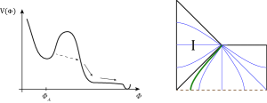
Figure 1: Left panel: A potential with a metastable de Sitter vacuum. Right panel: Penrose diagram for a bubble nucleated in de Sitter space. The horizontal line at the bottom represents a global slice in de Sitter space at the time of bubble nucleation. The green line is the bubble wall; on its left (right) is the true (ancestor) vacuum. Our universe is an open FLRW universe inside the bubble, represented as Region I.

In the previous paper Aoki:2017scu , five of the present authors proposed a model for dark energy, partially motivated by string landscape. Assuming our universe has been created by bubble nucleation from a metastable de Sitter space (the “ancestor vacuum”), residual effects of quantum fluctuations generated in the ancestor vacuum has been interpreted as the source of dark energy. Its equation of state parameter $w_{\rm DE}(z)$ has a characteristic form as a function of the redshift $z$. The purpose of the present Letter is to assess the possibility of observational tests of this model. Observations that we consider to be particularly promising are galaxy surveys by Square Kilometre Array (SKA) SKA and Euclid Euclid , planned to start operating in the early 2020’s. We will perform Fisher analysis and forecast the constraints for our model.

The theoretical setup.—

We consider bubble nucleation due to quantum tunneling, which occurs e.g., in a potential for a scalar field $\Phi$ shown in FIG. 1, left panel. The Hubble parameter of the ancestor vacuum will be denoted $H_{A}$. Our universe is inside the bubble, represented as Region I in FIG. 1, right panel. It should have negative spatial curvature Coleman:1980aw . After bubble nucleation, the ordinary inflation with the Hubble parameter $H_{I}(\ll H_{A})$ is assumed to occur.

We consider a scalar field $\phi$ which is different from the tunneling field $\Phi$ and has zero expectation value. We assume the field $\phi$ to have mass $m_{A}$ before tunneling, and $m_{0}$ after tunneling, where $m_{A}$ and $m_{0}$ could be different. The latter is assumed to satisfy $m_{0}\lesssim H_{0}$ where $H_{0}\sim 10^{-33}{\rm eV}$ is the present Hubble parameter. A candidate for such an ultralight field is one of the axion-like fields, expected to exist in string compactifications Arvanitaki:2009fg .

In Aoki:2017scu , the contribution from the field $\phi$ to the vacuum expectation value of the energy-momentum tensor $\langle T_{\mu\nu}\rangle$ has been computed, carefully taking into account the effect of the ancestor vacuum. In the free-field approximation, the energy-momentum tensor is quadratic in $\phi$, thus $\langle T_{\mu\nu}\rangle$ can be obtained by taking the coincident-point limit of the two-point function $\langle\phi\phi\rangle$ computed by the method developed in Yamamoto:1996qq ; Sasaki:1994yt ; Freivogel:2006xu . We refer the reader to Aoki:2017scu for details, and give an order-of-magnitude argument here. In the ancestor vacuum, quantum fluctuations give rise to the expectation value of the field-squared $\langle\phi^{2}\rangle\sim H_{A}^{4}/m_{A}^{2}$, as in pure de Sitter space (see e.g., Linde:2005ht ). The field $\phi$ is almost frozen until now, due to the assumption $m_{0}\lesssim H_{0}$ (and one more condition $\epsilon\ll 1$, to be mentioned below). If so, the energy-momentum tensor is dominated by the mass term, and takes the form of cosmological constant ($w_{\rm DE}=-1$), with the magnitude

$$\langle T_{\mu\nu}\rangle\sim m_{0}^{2}\langle\phi^{2}\rangle g_{\mu\nu}\sim H_{A}^{4}\left({m_{0}\over m_{A}}\right)^{2}g_{\mu\nu}\,.$$ (1)

It is not difficult for this to have the same order of magnitude as dark energy, $\rho_{\rm DE}\sim M_{P}^{2}H_{0}^{2}$, once we admit $m_{0}\sim H_{0}$: We just need $m_{A}/H_{A}\sim H_{A}/M_{P}$, i.e., $H_{A}$ being the geometric mean of $m_{A}$ and $M_{P}$.

Difference from quintessence.—

At the level of the above heuristic argument, it makes no difference whether $\phi$ is a classical or quantum field. However, fully quantum mechanical analysis in Aoki:2017scu has the following two important differences from the classical case.

First, there is no ambiguity in the initial condition for the field $\phi$, unlike in the classical case, in which one has to assign e.g., the axion misalignment angle by hand. Our prediction (1) is unambiguous when $H_{A}$, $m_{A}$, $m_{0}$ are given. This is a virtue of bubble nucleation, which allows us to go past the beginning of the FLRW time and uniquely determine the vacuum state of a quantum field.

Second, the mode of $\phi$ which gives the dominant contribution at late times is not strictly homogeneous. It is an eigenfunction of the Laplacian on the spatial slice $H^{3}$ with a non-zero eigenvalue. There is a peculiar feature of modes on a hyperboloid. Normalizable modes decay exponentially (since the volume grows exponentially) at large distances; they have eigenvalues $\nabla^{2}=-(k^{2}+1)$ with real $k$. However, in an open universe created by bubble nucleation, there is the so-called supercurvature mode Yamamoto:1996qq ; Sasaki:1994yt , which is non-normalizable on $H^{3}$, and has an eigenvalue with imaginary $k=i(1-\epsilon)$, i.e., $\nabla^{2}\sim-2\epsilon$ when $\epsilon\ll 1$. The parameter $\epsilon$ is determined by the properties of the ancestor vacuum,

$$\epsilon=c_{\epsilon}\left({m_{A}\over H_{A}}\right)^{2},$$ (2)

when $m_{A}/H_{A}\ll 1$, with an order-one coefficient $c_{\epsilon}$ which depends on the size of the critical bubbleAoki:2017scu . The supercurvature mode gives rise to long-range correlations in the open universe, which can be interpreted as the superhorizon fluctuations in the ancestor vacuum, seen from the inside of the bubble.

Observational signature.—

The energy-momentum tensor for $\phi$ at late times is dominated by the contribution from the supercurvature mode. The spatial derivative term in $\langle T_{\mu\nu}\rangle$ gives a non-zero contribution, $\langle(\nabla\phi)^{2}\rangle=-\langle\phi\nabla^{2}\phi\rangle\sim 2\epsilon\langle\phi^{2}\rangle$. If $\epsilon\ll 1$ and $m_{0}\ll H_{0}$ (though these inequalities do not have to be very strong, in practice), the time-derivative term is negligible Aoki:2017scu . Then, the EoS parameter $w_{\rm DE}$ can be obtained by simply taking the ratio of $p$ to $\rho$, and becomes

$$w_{\rm DE}=-{{2\over 3}(\epsilon/R_{c}^{2})+m_{0}^{2}a^{2}\over 2(\epsilon/R_{c}^{2})+m_{0}^{2}a^{2}}=-{1+{2\over 3}\tilde{\epsilon}(1+z)^{2}\over 1+2\tilde{\epsilon}(1+z)^{2}}\,.$$ (3)

where $R_{c}$ is the comoving radius of curvature, which is constant. The final expression shows that the functional form of $w_{\rm DE}(z)$ depends on a single parameter,

$$\tilde{\epsilon}\equiv{\epsilon\over(m_{0}/H_{0})^{2}}\Omega_{{\rm K},0}\equiv\xi\Omega_{\rm K,0}\,,$$ (4)

where $\Omega_{{\rm K},0}=1/H_{0}^{2}R_{c}^{2}$ is the fractional energy density of the spatial curvature at present. At late times, the mass term is dominant in (3), thus $w_{\rm DE}(z)\to-1$. At early times, the spatial derivative term becomes dominant, thus $w_{\rm DE}(z)\to-1/3$. The past asymptotic value $w_{\rm DE}(z)\to-1/3$ is unlikely to be realized in the ordinary inflation: $\langle T_{\mu\nu}\rangle$ in de Sitter space with a de Sitter invariant vacuum should have $w=-1$; evolution of wave functions after inflation will give rise to non-zero time derivatives, not only spatial derivatives.

We regard the functional form of $w_{\rm DE}(z)$ in (3) to be an indication of fluctuations generated before ordinary inflation, but in fact, this may not be specific to open universe or bubble nucleation. If an infrared part of the fluctuations is enhanced relative to the usual magnitude $H_{I}$ and is frozen until now, it will contribute to the spatial-derivative and mass terms of the energy-momentum tensor, giving the EoS parameter similar to (3). This can happen e.g., in a double inflation model in Aoki:2014ita ; Aoki:2014dqa .

Eq. (3) leads to a simple relation between $w_{0}$ and its derivative $w_{a}=-dw/da|_{a=1}$: When $\tilde{\epsilon}\ll 1$, we have $w_{a}=2(w_{0}+1)=8\tilde{\epsilon}/3$. This relation could be testable by ongoing observations such as Dark Energy Survey DES . This will be a first step toward testing our model.

Eq. (3) yields the energy density of dark energy as a function of the redshift,

$$\rho_{\rm DE}(z)=3M_{P}^{2}H_{0}^{2}\,\Omega_{\rm\Lambda,0}\left(1+2\widetilde{\epsilon}(1+z)^{2}\right)\,.$$ (5)

The mass term in the energy-momentum tensor gives the time-independent contribution $3M_{P}^{2}H_{0}^{2}\,\Omega_{\Lambda,0}$ to (5). The spatial derivative term gives a contribution with the relative factor $2\widetilde{\epsilon}(1+z)^{2}$. In terms of the model parameters, $\Omega_{\Lambda,0}$ is given by

$$\Omega_{\Lambda,0}=\frac{1}{6}\tilde{c}_{*}\frac{H_{A}^{4}}{H_{0}^{2}M_{P}^{2}}\left(\frac{m_{0}}{m_{A}}\right)^{2}\,,$$ (6)

with $\tilde{c}_{*}=c_{*}(H_{I}/H_{A})^{2\epsilon}$, where $c_{*}$ depends on the size of the critical bubble Aoki:2017scu . We can take $(H_{I}/H_{A})^{2\epsilon}\sim 1$ when $\epsilon$ is sufficiently small. The parameters $H_{A}$, $m_{A}$, $m_{0}$ in the model are related to the observables, $\Omega_{\Lambda,0}$ and $\xi$ as

$${H_{A}\over M_{P}}=\sqrt{6\xi\Omega_{\Lambda,0}\over\tilde{c}_{*}c_{\epsilon}}\,,\ \ {m_{A}\over M_{P}}=\sqrt{\frac{6\Omega_{\Lambda,0}}{\tilde{c}_{*}}}\,\frac{\xi}{c_{\epsilon}}\,\frac{m_{0}}{H_{0}}\,.$$ (7)

We will forecast the constraints for $\xi$, rather than $\tilde{\epsilon}=\xi\Omega_{K,0}$. Since the definition of $\xi$ is independent of $\Omega_{\rm K,0}$, it is not constrained to be very small; we expect $\xi={\cal O}(1)$ as a natural choice. If we can determine $\xi$ from observations, (7) allows us to determine an important parameter $H_{A}$.

Fisher analysis for galaxy surveys.—

SKA SKA is a ground based array of radio telescopes which covers about 3/4 of the sky and observes galaxies by detecting the 21cm emission line of neutral hydrogen. Euclid Euclid is a satellite based telescope working in the visible and near-infrared wavelength domains. SKA phase 2 (SKA2) and Euclid are both expected to observe a billion galaxies up to the redshift $z\sim 2$. In our analysis, we use the survey specifications described in Yahya:2014yva for SKA, and in Amendola:2016saw for Euclid. We take the power spectrum of galaxy distribution as an observable, and forecast the constraints on the parameters, following the standard procedure (see e.g., Tegmark:1997rp ; Seo:2003pu ; White:2008jy ; Yamauchi:2016ypt ).

As the fiducial cosmological model, we take a $w$CDM model whose dark energy is characterized by $w$ in (3) with the negative spatial curvature. The Hubble parameter $H(z)$ obeys

$$\frac{H^{2}}{H_{0}^{2}}=\Omega_{\rm m,0}(1+z)^{3}+\widetilde{\Omega}_{\rm K,0}(1+z)^{2}+\Omega_{\Lambda,0}\,,$$ (8)

$$\frac{\dot{H}}{H_{0}^{2}}=-\frac{3}{2}\Omega_{\rm m,0}(1+z)^{3}-\widetilde{\Omega}_{\rm K,0}(1+z)^{2}\,.$$ (9)

Interestingly, the spatial derivative term in the energy-momentum tensor contributes exactly in the same way as the spatial curvature to Eqs. (8) and (9), effectively replacing $\Omega_{\rm K,0}$ with $\widetilde{\Omega}_{\rm K,0}\equiv\left(1+2\xi\Omega_{\Lambda,0}\right)\Omega_{\rm K,0}$. Thus there is a tendency for degeneracy between $\Omega_{\rm K,0}$ and $\xi$. On the other hand, the angular diameter distance, $D_{\rm A}(z)=\left((1+z)H_{0}\sqrt{\Omega_{\rm K,0}}\right)^{-1}\sinh\left(H_{0}\sqrt{\Omega_{\rm K,0}}\int_{0}^{z}H^{-1}(z^{\prime})\mathrm{d}z^{\prime}\right)$, is defined in terms of the true curvature $\Omega_{\rm K,0}$. This fact is expected to break the degeneracy.

We consider a model for galaxy distribution in the linear regime. The matter density contrast $\delta_{\rm m}$ satisfies the $k$-independent equation at the linear level (see e.g., Peebles ),

$$\ddot{\delta}_{\rm m}+2H\dot{\delta}_{\rm m}-\frac{3}{2}H^{2}\Omega_{\rm m}\delta_{\rm m}=0\,.$$ (10)

An object of interest is the linear growth rate $f\equiv\frac{\mathrm{d}\ln\delta_{\rm m}}{\mathrm{d}\ln a}$. The observed galaxy power spectrum in the redshift space is well described by

$$P_{\rm g}({\bm{k}};z)=\left(b(z)+f(z)\mu^{2}\right)^{2}P_{\rm m}(k;z)e^{-k^{2}\mu^{2}\sigma_{\rm NL}^{2}}\,,$$ (11)

where $P_{\rm m}(k,z)$ is the linear matter power spectrum, and $b(z)$ is the so-called galaxy bias function, which should be chosen according to the type of target galaxies for the particular observation: for SKA, $b(z)=c_{1}\exp(c_{2}z)$ with constant $c_{1}$ and $c_{2}$; for Euclid, $b=\sqrt{1+z}$. The term $f\mu^{2}$, where $\mu$ is the cosine of the angle between the line of sight and the wave vector ${\bm{k}}$, represents the redshift space distortion Kaiser:1987qv , due to the contribution to the observed redshift from the peculiar velocity driven by the clustering of matter (making dense region look denser). The factor $e^{-k^{2}\mu^{2}\sigma_{\rm NL}^{2}}$ with a free parameter $\sigma_{\rm NL}\approx 7\,[{\rm Mpc}]$ to be marginalized, is introduced to represent the inaccuracies in the observed redshift, which results in the line-of-sight smearing. Further, taking into account the geometrical effects due to the difference between the possibly incorrect reference cosmology and the true one, the so-called Alcock-Paczynski (AP) effect Alcock:1979mp , the observed power spectrum is given by Seo:2003pu

$$P_{\rm obs}({\bm{k}}_{\perp}^{\rm ref},k_{\parallel}^{\rm ref};z)=\left(\frac{D_{\rm A}^{\rm ref}(z)}{D_{\rm A}(z)}\right)^{2}\frac{H(z)}{H^{\rm ref}(z)}P_{\rm g}({\bm{k}}_{\perp},k_{\parallel};z)\,.$$

Here the angular diameter distance $D_{\rm A}$ and the Hubble parameter $H$ in the reference cosmology are distinguished by the subscript ‘ref’, while those in true cosmology have no subscript. The wave number across and along the line-of-sight in the two cosmologies are related through $k_{\parallel}=\frac{H}{H^{\rm ref}}k_{\parallel}^{\rm ref}$ and ${\bm{k}}_{\perp}=\frac{D_{\rm A}^{\rm ref}}{D_{\rm A}}{\bm{k}}_{\perp}^{\rm ref}$.

The forecast.—

The Fisher matrix for a set of parameters $\{\theta^{\alpha}\}$ is defined as $F_{\alpha\beta}=\left\langle{\partial\over\partial\theta_{\alpha}}{\partial\over\partial\theta_{\beta}}\log{\cal L}\right\rangle$ where ${\cal L}$ is the likelihood function when we regard $\{\theta^{\alpha}\}$ as probabilistic variables which depends on the data set. The matrix $F_{\alpha\beta}$ is the inverse of the covariance matrix, and the minimum 1$\sigma$ error on $\theta_{\alpha}$ is given by $\sqrt{(F^{-1})_{\alpha\alpha}}$ (no sum on $\alpha$). In terms of galaxy power spectrum, the Fisher matrix can be written as Seo:2003pu ; Tegmark:1997rp

$$F_{\alpha\beta} =\sum_{z_{i}}\int_{k_{\rm min}}^{k_{\rm max}}\frac{\mathrm{d}^{3}{\bm{k}}}{(2\pi)^{3}}V_{\rm eff}({\bm{k}};z_{i})$$

$$\qquad\times\frac{\partial\ln P_{\rm obs}({\bm{k}};z_{i})}{\partial\theta^{\alpha}}\frac{\partial\ln P_{\rm obs}({\bm{k}};z_{i})}{\partial\theta^{\beta}}\,,$$ (12)

where the effective volume of the survey is given by

$$V_{\rm eff}({\bm{k}};z_{i})\approx\left(\frac{n_{\rm g}(z_{i})P_{\rm obs}({\bm{k}};z_{i})}{n_{\rm g}(z_{i})P_{\rm obs}({\bm{k}};z_{i})+1}\right)^{2}V_{\rm survey}(z_{i})\,.$$ (13)

The survey volume is divided into bins with the width $\Delta z=0.1$ in the redshift. Here $V_{\rm survey}(z_{i})$ is the comoving volume of the redshift slice centered at $z_{i}$. The minimum wavelength is $k_{\rm min}(z_{i})=2\pi/V_{\rm survey}^{1/3}(z_{i})$. The maximal wavelength is taken to be the scale beyond which non-linearities become non-negligible. It is estimated as $k_{\rm max}(z_{i})=0.14(1+z_{i})^{2/(2+n_{\rm s})}\,[{\rm Mpc}^{-1}]$.

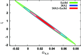
Figure 2: Forecast 1$\sigma$ and 2$\sigma$ marginal contours with the fiducial values $(\Omega_{\rm K,0},\xi)=(0.03,0.8)$ for SKA2 galaxy survey (blue), Euclid (green), and the combined analysis (red).

Our forecast is performed for the parameter set: $\{h,\Omega_{\Lambda,0},\Omega_{\rm K,0},h^{2}\Omega_{\rm b,0},\sigma_{8},n_{\rm s},\sigma_{\rm NL},b(z_{i})\}$ and $\{\xi\}$. The fiducial values are taken as $h=0.67,\ h^{2}\Omega_{\rm b,0}=0.0222,\ \Omega_{\Lambda,0}=0.6817,\ \sigma_{8}=0.834,\ n_{\rm s}=0.962,\ \Omega_{\rm K,0}=0.03,$ and $\xi=0.8$.

FIG. 2 shows the forecast 1$\sigma$ and 2$\sigma$ contour in the $(\Omega_{\rm K,0},\xi)$ plane for SKA2 and Euclid. There is degeneracy between $\Omega_{\rm K,0}$ and $\xi$ along the $\widetilde{\Omega}_{\rm K,0}=\text{const}$. direction, for the reason mentioned above. However, for this set of fiducial values of the parameters, one can see the difference from $\xi=0$ (i.e., time independent cosmological constant) at the 1$\sigma$ level.

Discussion.—

The above choice of parameters, $(\Omega_{\rm K,0},\xi)=(0.03,0.8)$, is barely consistent with the current constraint on the spatial curvature. These parameters may take smaller values. In that case, it might be difficult to determine these parameters solely from the results of galaxy surveys in the near future.

To break the degeneracy between $\Omega_{\rm K,0}$ and $\xi$, it is highly important to combine galaxy surveys with other observations of spatial curvature which have different dependence on the angular/luminosity/comoving distance. Possible detection of negative curvature by observations of the CMB will greatly improve the chance of determining the parameters, since the CMB involves larger $z$ than the galaxy surveys, and will be more sensitive to the angular diameter distance. On the other hand, positive curvature at the level of $\Omega_{\rm K,0}\lesssim-10^{-4}$ would falsify bubble nucleation, as argued in Kleban:2012ph , thus its detection would rule out our model.

If the results of galaxy surveys are consistent with our model with non-zero $\xi$, we may wonder whether this rules out other models. For instance, there is a quintessence model, called “scaling freezing” model, whose EoS parameter approaches $w_{\rm DE}\to-1$ in the future and $w_{\rm DE}\to 0$ in the past, and the transition occurs around $a\sim a_{t}$. Although it would be difficult for galaxy surveys at $z\lesssim 2$ to distinguish the past asymptotic values $w_{\rm DE}\to-1/3$ and $w_{\rm DE}\to 0$, in fact, there is already a strong constraint for the latter Chiba:2012cb ; Durrive:2018quo : The existing data of CMB, BAO, SNe, suggest that the transition has to occur quite early $a_{t}<0.11$ (i.e., $z>8.1$). Thus, the model with the past asymptotic behavior $w_{\rm DE}\to 0$ should have $w_{\rm DE}\approx-1$ at $z\lesssim 2$, and cannot be responsible for the possible deviation from $w_{\rm DE}=-1$ discussed in this Letter.

References

- (1) H. Aoki, S. Iso, D. S. Lee, Y. Sekino and C. P. Yeh, Phys. Rev. D 97, no. 4, 043517 (2018) [arXiv:1710.09179 [hep-th]].
- (2) S. Perlmutter et al. [Supernova Cosmology Project Collaboration], Astrophys. J. 517, 565 (1999) [astro-ph/9812133].
- (3) A. G. Riess et al. [Supernova Search Team], Astron. J. 116, 1009 (1998) [astro-ph/9805201].
- (4) D. H. Weinberg, M. J. Mortonson, D. J. Eisenstein, C. Hirata, A. G. Riess and E. Rozo, Phys. Rept. 530, 87 (2013) [arXiv:1201.2434 [astro-ph.CO]].
- (5) P. A. R. Ade et al. [Planck Collaboration], Astron. Astrophys. 594, A13 (2016) [arXiv:1502.01589 [astro-ph.CO]].
- (6) P. A. R. Ade et al. [Planck Collaboration], Astron. Astrophys. 594, A14 (2016) [arXiv:1502.01590 [astro-ph.CO]].
- (7) L. Amendola and S. Tsujikawa, “Dark Energy : Theory and Observations,” Cambridge University Press.
- (8) https://www.skatelescope.org/
- (9) http://sci.esa.int/euclid/
- (10) K. Kohri, Y. Oyama, T. Sekiguchi and T. Takahashi, JCAP 1702, no. 02, 024 (2017) [arXiv:1608.01601 [astro-ph.CO]].
- (11) S. R. Coleman and F. De Luccia, Phys. Rev. D 21, 3305 (1980).
- (12) J. Garriga, X. Montes, M. Sasaki and T. Tanaka, Nucl. Phys. B 551, 317 (1999) [astro-ph/9811257].
- (13) T. Tanaka and M. Sasaki, Prog. Theor. Phys. 97, 243 (1997) [astro-ph/9701053].
- (14) D. Yamauchi, T. Fujita and S. Mukohyama, JCAP 1403, 031 (2014) [arXiv:1402.2784 [astro-ph.CO]].
- (15) B. Freivogel, M. Kleban, M. Rodriguez Martinez and L. Susskind, JHEP 0603, 039 (2006) [hep-th/0505232].
- (16) A. Arvanitaki, S. Dimopoulos, S. Dubovsky, N. Kaloper and J. March-Russell, Phys. Rev. D 81, 123530 (2010) [arXiv:0905.4720 [hep-th]].
- (17) A. D. Linde, M. Sasaki and T. Tanaka, Phys. Rev. D 59, 123522 (1999) [astro-ph/9901135].
- (18) D. Yamauchi, A. Linde, A. Naruko, M. Sasaki and T. Tanaka, Phys. Rev. D 84, 043513 (2011) [arXiv:1105.2674 [hep-th]].
- (19) K. Sugimura, D. Yamauchi and M. Sasaki, EPL 100, no. 2, 29004 (2012) [arXiv:1208.3937 [astro-ph.CO]].
- (20) K. Sugimura, D. Yamauchi and M. Sasaki, JCAP 1201, 027 (2012) [arXiv:1110.4773 [gr-qc]].
- (21) K. Yamamoto, M. Sasaki and T. Tanaka, Phys. Rev. D 54, 5031 (1996) [astro-ph/9605103].
- (22) M. Sasaki, T. Tanaka and K. Yamamoto, Phys. Rev. D 51, 2979 (1995) [gr-qc/9412025].
- (23) B. Freivogel, Y. Sekino, L. Susskind and C. P. Yeh, Phys. Rev. D 74, 086003 (2006) [hep-th/0606204].
- (24) A. D. Linde, “Particle physics and inflationary cosmology,” CRC press, 1990 [hep-th/0503203].
- (25) S. Hannestad and E. Mortsell, JCAP 0409, 001 (2004) [astro-ph/0407259].
- (26) H. Aoki, S. Iso and Y. Sekino, Phys. Rev. D 89, no. 10, 103536 (2014) [arXiv:1402.6900 [hep-th]].
- (27) H. Aoki and S. Iso, PTEP 2015, no. 11, 113E02 (2015) [arXiv:1411.5129 [gr-qc]].
- (28) https://www.darkenergysurvey.org/
- (29) S. Yahya, P. Bull, M. G. Santos, M. Silva, R. Maartens, P. Okouma and B. Bassett, Mon. Not. Roy. Astron. Soc. 450, no. 3, 2251 (2015) [arXiv:1412.4700 [astro-ph.CO]].
- (30) L. Amendola et al., Living Rev. Rel. 21, no. 1, 2 (2018) [arXiv:1606.00180 [astro-ph.CO]].
- (31) N. Kaiser, Mon. Not. Roy. Astron. Soc. 227, 1 (1987).
- (32) M. White, Y. S. Song and W. J. Percival, Mon. Not. Roy. Astron. Soc. 397, 1348 (2008) [arXiv:0810.1518 [astro-ph]].
- (33) H. J. Seo and D. J. Eisenstein, Astrophys. J. 598, 720 (2003) [astro-ph/0307460].
- (34) C. Alcock and B. Paczynski, Nature 281, 358 (1979).
- (35) M. Tegmark, Phys. Rev. Lett. 79, 3806 (1997) [astro-ph/9706198].
- (36) D. Yamauchi et al. [SKA-Japan Consortium Cosmology Science Working Group], PoS DSU 2015, 004 (2016) [Publ. Astron. Soc. Jap. 68, no. 6, R2 (2016)] [arXiv:1603.01959 [astro-ph.CO]].
- (37) P.J.E. Peebles, ‘Large Scale Structure of the Universe,’ Princeton University Press.
- (38) M. Kleban and M. Schillo, JCAP 1206, 029 (2012) [arXiv:1202.5037 [astro-ph.CO]].
- (39) T. Chiba, A. De Felice and S. Tsujikawa, Phys. Rev. D 87, no. 8, 083505 (2013) [arXiv:1210.3859 [astro-ph.CO]].
- (40) J. B. Durrive, J. Ooba, K. Ichiki and N. Sugiyama, Phys. Rev. D 97, no. 4, 043503 (2018) [arXiv:1801.09446 [astro-ph.CO]].