Ultrahigh-precision measurement of the $n$$=$$2$ triplet P fine structure of atomic helium using frequency-offset separated oscillatory fields

Abstract

For decades, improved theory and experiment of the $n$$=$$2$ ³P fine structure of helium have allowed for increasingly-precise tests of quantum electrodynamics, determinations of the fine-structure constant $\alpha$, and limitations on possible beyond-the-Standard-Model physics. Here we use the new frequency-offset separated-oscillatory-fields (FOSOF) technique to measure the $2^{3}$P${}_{2}\!\!\to\!2^{3}$P₁ interval. Our result of $2\,291\,176\,590(25)$ Hz represents a major step forward in precision for helium fine-structure measurements.

PACS numbers

\pacs{32.70.Jz,32.80.-t}

In 1964, Schwartz suggested Schwartz (1964) that a part-per-million (ppm) determination of the fine-structure constant $\alpha$ might be possible using the 2³P fine structure of atomic helium if advances were made to both theory and experiment. In the past five decades, great progress has indeed been made in experimental measurements Pichanick et al. (1968); Kponou et al. (1971, 1981); Frieze et al. (1981); Shiner et al. (1994); Shiner and Dixson (1995); Castillega et al. (2000); Smiciklas and Shiner (2010); Prevedelli et al. (1996); Minardi et al. (1999); Pastor et al. (2004, 2006); Giusfredi et al. (2005); Zelevinsky et al. (2005); Storry and Hessels (1998); Storry et al. (2000); George et al. (2001); Borbely et al. (2009); Feng et al. (2015); Zheng et al. (2017) (including the evaluation of new systematic effects Marsman et al. (2012a, b, 2014, 2015a, 2015b)) and in the quantum-electrodynamic (QED) theory Schiff et al. (1965); Kim (1965); Hambro (1972a, b, 1973); Douglas and Kroll (1974); Daley et al. (1972); Lewis and Serafino (1978); Yan and Drake (1995); Zhang (1996a, b); Zhang et al. (1996); Drake (2002); Pachucki and Sapirstein (2000, 2003); Sapirstein (2010); Pachucki (1999, 2006); Pachucki and Yerokhin (2009a, b, 2010, 2011, 2012); Pei-Pei et al. (2015) of these intervals. The present measurement of the $2^{3}$P${}_{2}\!\!\to\!2^{3}$P₁ interval has an uncertainty of only 25 Hz, which, when compared to the full 31.9 GHz 2³P fine structure, for the first time reaches below one part per billion (ppb). Thus, the present measurement is the first building block towards using the 2³P fine structure for tests of physics and fundamental constants at the $<$1-ppb level. The other building blocks necessary will be a measurement of the the $2^{3}$P${}_{1}\!\!\to\!2^{3}$P₀ interval (which can be done with the same method demonstrated in this work) and an advance of QED theory to this same level of accuracy. The latter will require extending the already heroic calculation of Pachucki and Yerokhin Pachucki and Yerokhin (2010) to one order higher in $\alpha$.

The payoff from assembling all of the building blocks will be large. First, the comparison between experiment and theory will provide the most accurate test to date of QED in a multielectron system Pachucki et al. (2017). Second, a $<$1-ppb test of the 2³P fine structure will directly test (at 100 times the current accuracy) for beyond-the-Standard-Model physics Pachucki et al. (2017), such as exotic spin-dependent interactions between electrons Ficek et al. (2017). Third, the combination of $<$1-ppb theory and experiment would allow for a determination of the $\alpha$ at a level of $<$0.5 ppb, which is approaching the level of the current best determinations of $\alpha$ based on the electron magnetic moment ($g_{e}$) Hanneke et al. (2008); Aoyama et al. (2012); Laporta (2017); Aoyama et al. (2018) and atomic recoil Parker et al. (2018); Bouchendira et al. . Comparing values of $\alpha$ determined from various systems allows for tests of beyond-the-Standard-Model physics in each of the systems Bouchendira et al. ; Hanneke et al. (2008). In particular, the $g_{e}$ measurement, given another determination of $\alpha$, becomes a 0.25-ppb test of QED, and tests for possible substructure of the electron Bouchendira et al. ; Gabrielse et al. (2014) and the possible presence of dark photons Bouchendira et al. ; Hanneke et al. (2008); Kahn et al. (2017), and puts limits on possible dark axial vector bosons Bouchendira et al. ; Hanneke et al. (2008). The recoil measurement, along with another $\alpha$ determination, could be used for an absolute mass standard Lan et al. (2013).

The current work is the first implementation of the new frequency-offset separated-oscillatory-fields (FOSOF) technique Vutha and Hessels (2015), which is a modification of the Ramsey method Ramsey (1949) of separated oscillatory fields (SOF). For FOSOF, the frequencies of the two separated fields are slightly offset from each other, so that the relative phase of the two fields varies continuously with time.

Our measurement uses a beam of metastable 2³S atoms created in a liquid-nitrogen-cooled DC discharge source. Two-dimensional magneto-optical trapping (2DMOT), using permanent magnets and interactions with 1083-nm laser beams from the four transverse directions (that interact for 20 cm along the atomic beam) concentrates the beam to a flux of 2³S atoms of 7$\times$10¹²/cm²/s. The atoms in this beam are optically pumped (OP in Fig. 1) into the 2³S($m$=$-$1) state before passing through a 0.5-mm-high slit into a coaxial microwave airline. The measurement takes place inside this airline. The 2³S($m$=$-$1) atoms are excited by a 15-ns pulse of 1083-nm laser light (A in Fig. 1) up to the 2³P₁($m$=$-$1) state. The $2^{3}$P${}_{1}(m$=$-$1$)\!\!\to\!2^{3}$P${}_{2}(m$=$-$1) transition is then driven with microwaves. The resulting 2³P${}_{2}(m$=$-$1) atoms are detected by exciting them up to 4³D₃($m$=$-$1) using a 50-ns pulse of linearly-polarized 447-nm laser light (B in Fig. 1), and then to 18³P₂($m$=$-$1) using a 80-ns pulse of linearly-polarized 1532-nm light (C in Fig. 1). The 18³P₂ atoms are Stark-ionized by electric fields created using the wires shown in Fig. 1(c), and the resulting ions are focused through a 1-mm slit into a channel electron multiplier (CEM). The CEM current is dominated by ions created by these steps, with only a very small background from collisional ionization at our ultra-high-vacuum pressure of 3$\times$10^-9 torr.

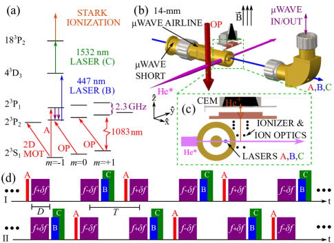
Figure 1: The experimental setup for the measurement. An energy-level diagram (a) shows the 2.3-GHz interval being measured and the laser transitions used. The experimental setup (b), along with an expanded view of the region where the measurement takes place (c) shows the laser and microwave interactions and ionization detection. The timing diagrams (d) show the FOSOF microwave pulses.

All three wavelengths are produced using diode lasers. The 1083-nm and 1532-nm light is amplified using fiber amplifiers. The pulses are created using double passes through acousto-optic modulators. The transition being measured is driven with two pulses of microwaves, each of duration $D$, and separated in time by $T$, as shown in Fig. 1(d). The pulses are created by fast switching of outputs from two precision microwave generators, with their internal clocks locked to each other and referenced to both Rb and GPS clocks. The microwaves enter one end of the airline, and reflect off of a short to form a standing wave. The returning wave is monitored on a power detector and an oscilloscope. The microwave frequencies of the pulses are offset by $\pm\delta\!f$, with pulses alternating between $f$$+$$\delta\!f$ and $f$$-$$\delta\!f$. The offset frequency $\delta\!f$ causes the relative phases of the two pulses to vary continuously in time. As a result, the atomic signal (see Fig. 2(a)) varies sinusoidally in time, cycling between destructive and constructive interference. The phase difference $\Delta\theta$ between this signal and a beat signal obtained by combining the microwaves at the two frequencies is shown in Fig. 2(a). We take data with two different timing sequences (Fig. 1(d)): with the $f$$+$$\delta\!f$ pulse before the $f$$+$$\delta\!f$ pulse (I), and vice versa (II). To switch from I to II, only the timing of the laser pulses is changed – the microwave pulses are untouched. Fig. 2(a) shows that the direction of the phase shift $\Delta\theta$ is opposite for the two cases, and, as a result, the average $\overline{\Delta\theta}$=($\Delta\theta_{I}$$-$$\Delta\theta_{II}$)/2 cancels unintended phase shifts due to lags in either the atomic or beat signals Vutha and Hessels (2015).

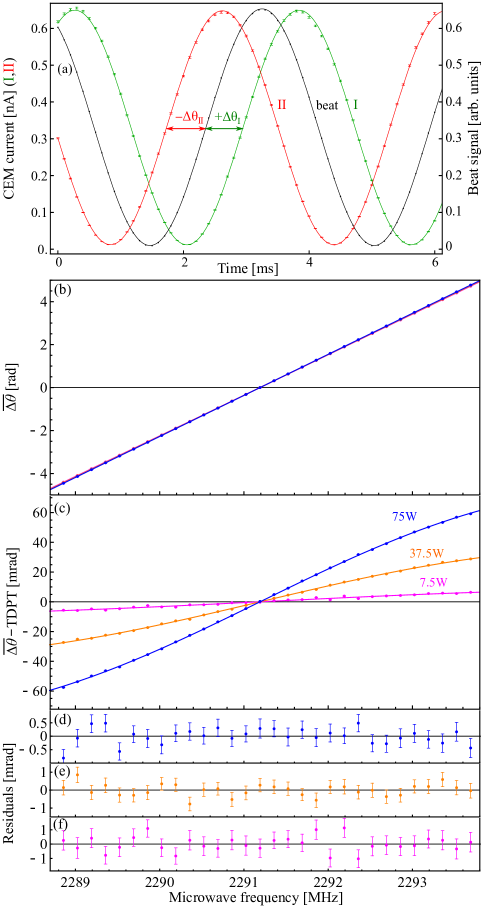
Figure 2: The FOSOF lineshape. The sinusoidal atomic signals for case I and II of Fig. 1(d) are shifted by $\Delta\theta_{I}$ and $\Delta\theta_{II}$ relative to a microwave beat signal, as shown in (a). The average phase shift $\overline{\Delta\theta}$ is shown in (b) for powers of 7.5, 37.5, and 75 W. A 100 times expanded scale in (c), where the straight-line predicted by TDPT is subtracted, resolves the lineshapes for different powers. The fits in (c) use Eq. (1), and the residuals from the fits are shown in (d), (e), and (f).

For the simple case of a two-level system with two ideal pulses of duration $D$ and separation $T$, the Schr$\ddot{\rm o}$dinger equation predicts a FOSOF lineshape $\overline{\Delta\theta}(f)$ of

$$\Delta\omega(T\!-\!D)\!+\!2\tan\!^{-1}\!\big{[}\frac{\Delta\omega\tan(\sqrt{4V^{2}\!+\!\Delta\omega^{2}}D/2)}{\sqrt{4V^{2}\!+\!\Delta\omega^{2}}}\big{]},$$ (1)

where $V$ is the magnetic-dipole matrix element driving the transition, and $\Delta\omega$/2$\pi$$=$$f$$-$$f_{0}$ is the separation between the applied microwave frequency and the atomic resonant frequency. This line shape is antisymmetric with respect to $\Delta\omega$, and reduces to simply $\Delta\omega T$ for small $V$, as can also be derived from time-dependent perturbation theory (TDPT). The observed lineshape is shown in Fig. 2(b) for the case of $T$$=$300 ns and $D$$=$100 ns for three different powers, $P$. The three powers give almost-identical, almost-linear lineshapes. On a 100-times expanded scale in Fig. 2(c), where the TDPT straight line has been subtracted, one can see that the data is described well by the lineshape of Eq. (1).

The signal-to-noise ratio (S/N) for the measurement is astonishingly good, due to the large number of metastable atoms afforded by the 2DMOT, due to the near-unity efficiency for detection via Stark ionization, and due to the lack of a background in our signal, which leads to uncertainties limited only by the shot noise in the signal itself. The excellent S/N can be seen directly in Fig. 2(a), where each point is an average of 20 ms of data. Note that the uncertainties in these plots are considerably larger at the top of the sinusoidal signal than at the bottom, as the shot-noise limited uncertainties are proportional to the square root of the signal size. The resulting lineshapes of Fig. 2(b), also show the excellent S/N, with each point representing 40 s of data. A fit to the 75-W data gives an $f_{0}$ determination with an uncertainty of only 30 Hz. This excellent S/N is despite the fact that measurement sequence takes 450 ns (much longer than the 98-ns 2³P lifetime), allowing only $e^{-(450\,{\rm ns})/(98\,{\rm ns})}$=1.0% of the 2³P atoms to contribute to the signal. The excellent S/N allows for a $T$ of up to 900 ns, where only 22 ppm of the 2³P atoms contribute. When all of the data used for this measurement is averaged, the statistical uncertainty is $<$2 Hz.

Our experiment is performed within a magnetic field $\vec{B}$ of typically 5 gauss. This $\vec{B}$ is applied by 20-cm-radius Helmholtz coils, with geomagnetic and other local fields canceled by six larger coils. The largest systematic effect in our measurement is a second-order Zeeman shift of 429.5 Hz/gauss². The quadratic shift rate is precisely calculated Yan and Drake (1994), and has been directly tested by other measurements Lewis et al. (1970); Zelevinsky et al. (2005) using larger $B$. We also use larger $B$ to directly show that we understand the magnetic shifts at a level of $<$0.1%, and we include a 0.1% uncertainty to all Zeeman corrections. Fig 4(a) shows that that measurements taken with $\vec{B}$ in the $+\hat{z}$ and $-\hat{z}$ directions agree, and that those with $|\vec{B}|$$<$5 gauss agree with those taken for $|\vec{B}|$$>$10 gauss (which have, on average, a six times larger Zeeman shift).

Eq. (1) assumes perfect microwave pulses, including sudden turn-on and turn-off, no chirp in the phase due to the microwave switching, and no changes in intensity or phase profiles as a function of $f$. Imperfections in the pulses cause the second largest systematic in our measurement. In our previous SOF measurement Borbely et al. (2009), we monitored the microwave pulses by directly digitizing them with an oscilloscope and attempted to determine shifts that result from pulse imperfections by integrating the Schr$\ddot{\rm o}$dinger equation using the recorded microwave pulses. Because of the excellent S/N, in this work, we could test such corrections directly, by varying both the power $P$ and the magnitude of the imperfections. Unfortunately, for both SOF and FOSOF measurements, we find the calculated corrections to be unreliable, with the corrected centers from different distortions and $P$ disagreeing at the level of several hundred Hz. We attribute this inconsistency to a combination of two factors: that the oscilloscope does not faithfully render the microwave pulse sent to it, and that the atoms do not see the same microwave profile as the oscilloscope (due, e.g., to impedance mismatches and resulting reflections and interferences).

Extensive modeling, however, shows that any form of distortion gives shifts that vary linearly with $P$. We find that FOSOF shifts extrapolate exactly to zero in the TDPT ($P$$\to$0) limit, but SOF shifts are only within $\sim$200 Hz of zero for $P$$\to$0. As a result of this modeling, the strategy used here is to extrapolate our FOSOF centers to $P$$=$0, as shown, e.g., in Fig 3. These extrapolations also account for small ($<$40 Hz) AC Zeeman shifts, and for AC Stark shifts, which are even smaller here because the beam passes through the standing wave at a node for the microwave electric field (an anti-node for the magnetic field). Measurements are repeated for combinations of $T$ and $D$ to confirm that all sets of parameters extrapolate to a single intercept, as shown in Fig. 4(b). Fig. 4(c) and (d) give averages for each $T$ and $D$, respectively. Both in the modeling and data, the extrapolations have slopes that vary approximately as $D/T$, and we could fit the data by using one extrapolation constant for each $D$ used in this experiment (as shown in Fig 3). Some data are also taken with larger imperfections which led to three-times-larger slopes for all extrapolations, but still obtained consistent intercepts within the 100 Hz accuracy of the test. As $P$ increases, the FOSOF signal starts to saturate, and the shifts no longer follow a linear trend. We use only data well below saturation in our fits, Fig. 4(e) shows that our results are independent of how strongly we enforce this saturation limit (by restricting $P\,D^{2}$$<$0.9, 0.75, 0.6, 0.45, or 0.3 W$\mu$s²).

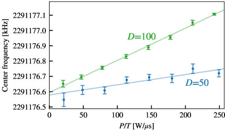
Figure 3: The extrapolation of the averaged $D$$=$100 ns and $D$$=$50 ns FOSOF fit centers to $P$$=$0, where the center is unaffected by imperfections in the pulses.

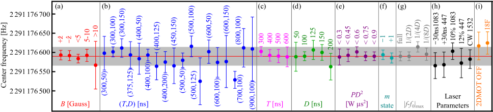
Figure 4: A summary of the average obtained center value for the various values of the experimental parameters. Details are explained in the text. All points use the saturation restriction of $PD^{2}$$<$0.75 W$\mu$s², the frequency range $|f-f_{0}|$$<$$1/(2D)$, and the magnetic field restriction $|\vec{B}|$$<$10 gauss, unless otherwise specified.

It is clear that our previous SOF data Borbely et al. (2009) should not have been corrected based on the oscilloscope traces, but rather should have been extrapolated to $P$=0. Using this method, the result from that work Borbely et al. (2009) changes from $2\,291\,177\,530(350)$ Hz to $2\,291\,176\,655(660)$ Hz.

The polarization for the optical-pumping step is reversed for half of the measurements, allowing the $2^{3}$P${}_{1}(m$=$+1)\!\!\to\!2^{3}$P${}_{2}(m$=$+$1) transition to also be measured. Fig. 4(f) shows that consistent results are obtained with $m$$=$$\pm 1$. To test for possible FOSOF lineshape effects, the data are also refit with only the central frequencies ($|f$$-$$f_{0}|$$<$$1/(2D)$, $1/(4D)$, or $1/(8D)$) included in the fit. Consistent results are found, as shown in Fig. 4(g). Data taken with up to 25 times higher pressure show no indication of a pressure shift and limits a possible shift to $<$4 Hz.

One concern is that the 18³P atoms travel through the rest of the airline before being ionized, and therefore they are exposed to additional microwave pulses which could drive atomic processes involving these states. To test for a systematic shift due to such processes, measurements are taken with lower duty cycles, with sufficient time between the FOSOF cycles to allow the 18³P atoms to exit without seeing additional microwave pulses. Additionally, measurements are performed in which the laser and microwave excitations are moved to the other side of the inner conductor of the airline of Fig. 1(c), so that the 18³P atoms spend far more time in the microwave fields. Finally, measurements are performed using the 18³F state instead of 18³P state (Fig. 4(h)). All three tests show that the $n$=18 states play no significant role.

To test for light shifts due to unintended temporal overlap of the laser and microwave pulses, data are taken at 8 times smaller 447-nm power, 10 times smaller 1083-nm power, with the 1532-nm laser on throughout the whole measurement sequence of Fig. 1(d), and by taking data with larger time delays between the laser and microwave pulses. In all cases, Fig. 4(i), the results indicate no light shifts. Consistent centers are also found for different offset frequencies: -2.8 kHz$<$$\delta\!f$$<$2.8 kHz. Also, different source temperatures (110 K to 300 K), different currents driving the DC discharge (10 mA to 25 mA), and not using the 2DMOT (Fig. 4(h)) reveal no inconsistencies.

Since this measurement is a first demonstration of the FOSOF method, we performed a parallel SOF experiment, in which we used the same microwave system as the one we used in Ref. Borbely et al. (2009), and the same laser cooling and detection method as applied here. Also, the magnitude and phase of the sinusoidal signals seen in the present FOSOF measurements (e.g., those in Fig. 2(b) and (c)) can be used to construct SOF data points, and these points can be fit to an SOF lineshape to find $f_{0}$. The $f_{0}$ obtained in this manner are less precise than the FOSOF $f_{0}$. Results for both SOF analyses (when extrapolated to $P$$=$0) agree with our present result to within 200 Hz – the level of agreement that we would expect since our modeling shows that SOF centers have a residual systematic shift even at $P$$=$0.

The weighted average of the results shown in Fig. 4(b) is $2\,291\,176\,590(11)_{\rm ext}(8)_{B}$ Hz, where the two uncertainties come from the extrapolations to $P$$=$0 and from the Zeeman shift. Based on the level of consistency demonstrated for a wide range of parameters in Fig. 4, we conservatively assign a larger uncertainty of $\pm$25 Hz to our measurement, giving a final measurement result of

$$[E(2^{3}{\rm P}_{1})-E(2^{3}{\rm P}_{2})]/h=2\,291\,176\,590(25)~{}{\rm Hz}.$$ (2)

Our result is slightly smaller (1.5 times the estimated theoretical uncertainty) than the best theoretical prediction Pachucki and Yerokhin (2010), as seen in Fig. 5. It disagrees with recent laser measurements by Hu, et al. Zheng et al. (2017); Feng et al. (2015) by 4.9 and 2.9 times their uncertainties. Only after the correction applied in this work does our previous SOF measurement Borbely et al. (2009) agree with the present measurement. With the inclusion of quantum interference corrections Marsman et al. (2015a, 2012b), the saturated-absorption measurement of Gabrielse, et al. Zelevinsky et al. (2005) and the the laser measurement of Shiner, et al. Smiciklas and Shiner (2010) also agree with the present measurement.

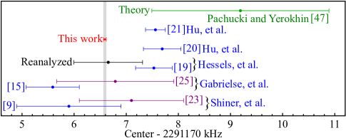
Figure 5: A comparison of the present measurement to previous measurements Zheng et al. (2017); Feng et al. (2015); Borbely et al. (2009); Zelevinsky et al. (2005); Smiciklas and Shiner (2010) and to theory Pachucki and Yerokhin (2010) Corrected centers including quantum interference effects Marsman et al. (2012b, 2015a) are also shown. The reanalyzed center from our previous SOF measurement as discussed in this work, is also shown.

This measurement is the most precise measurement to date of helium fine structure, and represents a major advance in this precision. The outstanding signal-to-noise ratio has allowed for a very extensive survey of systematic effects. This work sets the stage for the a new level of accuracy for this fine structure, which, when combined with more precise theory, could provide $<$1 ppb tests of the physics and constants relevant to the interval – including a precise determination of the fine-structure constant, the most precise test of QED in a multi-electron system, and tests for physics beyond the Standard Model.

This work is supported by NSERC, CRC, ORF, CFI, NIST and a York University Research Chair. We thank Amar Vutha, Daniel Fitzakerley, Matthew George, Hermina Beica, Travis Valdez, Nikita Bezginov, and Cody Storry for their contributions to this work.

References

- Schwartz (1964) C. Schwartz, Phys. Rev. 134, A1181 (1964).
- Pichanick et al. (1968) F. M. J. Pichanick, R. D. Swift, C. E. Johnson, and V. W. Hughes, Phys. Rev. 169, 55 (1968).
- Kponou et al. (1971) A. Kponou, V. W. Hughes, C. E. Johnson, S. A. Lewis, and F. M. J. Pichanick, Phys. Rev. Lett. 26, 1613 (1971).
- Kponou et al. (1981) A. Kponou, V. W. Hughes, C. E. Johnson, S. A. Lewis, and F. M. J. Pichanick, Phys. Rev. A 24, 264 (1981).
- Frieze et al. (1981) W. Frieze, E. A. Hinds, V. W. Hughes, and F. M. J. Pichanick, Phys. Rev. A 24, 279 (1981).
- Shiner et al. (1994) D. Shiner, R. Dixson, and P. Zhao, Phys. Rev. Lett. 72, 1802 (1994).
- Shiner and Dixson (1995) D. L. Shiner and R. Dixson, IEEE Trans. Instr. Meas. 44, 518 (1995).
- Castillega et al. (2000) J. Castillega, D. Livingston, A. Sanders, and D. Shiner, Phys. Rev. Lett. 84, 4321 (2000).
- Smiciklas and Shiner (2010) M. Smiciklas and D. Shiner, Phys. Rev. Lett. 105, 123001 (2010).
- Prevedelli et al. (1996) M. Prevedelli, P. Cancio, G. G, F. S. Pavone, and I. M, Opt. Comm. 125, 231 (1996).
- Minardi et al. (1999) F. Minardi, G. Bianchini, P. C. Pastor, G. Giusfredi, F. S. Pavone, and M. Inguscio, Phys. Rev. Lett. 82, 1112 (1999).
- Pastor et al. (2004) P. C. Pastor, G. Giusfredi, P. D. Natale, G. Hagel, C. de Mauro, and M. Inguscio, Phys. Rev. Lett. 92, 023001 (2004).
- Pastor et al. (2006) P. C. Pastor, G. Giusfredi, P. De Natale, G. Hagel, C. de Mauro, and M. Inguscio, Phys. Rev. Lett. 97, 139903 (2006).
- Giusfredi et al. (2005) G. Giusfredi, P. C. Pastor, P. D. Natale, D. Mazzotti, C. d. Mauro, L. Fallani, G. Hagel, V. Krachmalnicoff, and M. Inguscio, Can. J. Phys. 83, 301 (2005).
- Zelevinsky et al. (2005) T. Zelevinsky, D. Farkas, and G. Gabrielse, Phys. Rev. Lett. 95, 203001 (2005).
- Storry and Hessels (1998) C. H. Storry and E. A. Hessels, Phys. Rev. A 58, R8 (1998).
- Storry et al. (2000) C. H. Storry, M. C. George, and E. A. Hessels, Phys. Rev. Lett. 84, 3274 (2000).
- George et al. (2001) M. C. George, L. D. Lombardi, and E. A. Hessels, Phys. Rev. Lett. 87, 173002 (2001).
- Borbely et al. (2009) J. S. Borbely, M. C. George, L. D. Lombardi, M. Weel, D. W. Fitzakerley, and E. A. Hessels, Phys. Rev. A 79, 060503 (2009).
- Feng et al. (2015) G.-P. Feng, X. Zheng, and S.-M. Hu, Phys. Rev. A 91, 030502 (2015).
- Zheng et al. (2017) X. Zheng, Y. R. Sun, J.-J. Chen, W. Jiang, K. Pachucki, and S.-M. Hu, Phys. Rev. Lett. 118, 063001 (2017).
- Marsman et al. (2012a) A. Marsman, M. Horbatsch, and E. A. Hessels, Phys. Rev. A 86, 012510 (2012a).
- Marsman et al. (2012b) A. Marsman, M. Horbatsch, and E. A. Hessels, Phys. Rev. A 86, 040501 (2012b).
- Marsman et al. (2014) A. Marsman, E. A. Hessels, and M. Horbatsch, Phys. Rev. A 89, 043403 (2014).
- Marsman et al. (2015a) A. Marsman, M. Horbatsch, and E. A. Hessels, Phys. Rev. A 91, 062506 (2015a).
- Marsman et al. (2015b) A. Marsman, M. Horbatsch, and E. A. Hessels, J. Phys. and Chem. Ref. Data 44, 031207 (2015b).
- Schiff et al. (1965) B. Schiff, C. L. Pekeris, and H. Lifson, Phys. Rev. 137, A1672 (1965).
- Kim (1965) K. Y. Kim, Phys. Rev. 140, A1498 (1965).
- Hambro (1972a) L. Hambro, Phys. Rev. A 5, 2027 (1972a).
- Hambro (1972b) L. Hambro, Phys. Rev. A 6, 865 (1972b).
- Hambro (1973) L. Hambro, Phys. Rev. A 7, 479 (1973).
- Douglas and Kroll (1974) M. Douglas and N. M. Kroll, Ann. Phys. (N.Y.) 82, 89 (1974).
- Daley et al. (1972) J. Daley, M. Douglas, L. Hambro, and N. M. Kroll, Phys. Rev. Lett. 29, 12 (1972).
- Lewis and Serafino (1978) M. L. Lewis and P. H. Serafino, Phys. Rev. A 18, 867 (1978).
- Yan and Drake (1995) Z.-C. Yan and G. W. F. Drake, Phys. Rev. Lett. 74, 4791 (1995).
- Zhang (1996a) T. Zhang, Phys. Rev. A 54, 1252 (1996a).
- Zhang (1996b) T. Zhang, Phys. Rev. A 53, 3896 (1996b).
- Zhang et al. (1996) T. Zhang, Z.-C. Yan, and G. W. F. Drake, Phys. Rev. Lett. 77, 1715 (1996).
- Drake (2002) G. W. F. Drake, Can. J. Phys. 80, 1195 (2002).
- Pachucki and Sapirstein (2000) K. Pachucki and J. Sapirstein, J. Phys. B 33, 5297 (2000).
- Pachucki and Sapirstein (2003) K. Pachucki and J. Sapirstein, J. Phys. B 36, 803 (2003).
- Sapirstein (2010) J. Sapirstein, J. Phys. B 43, 074015 (2010).
- Pachucki (1999) K. Pachucki, J. Phys. B 32, 137 (1999).
- Pachucki (2006) K. Pachucki, Phys. Rev. Lett. 97, 013002 (2006).
- Pachucki and Yerokhin (2009a) K. Pachucki and V. A. Yerokhin, Phys. Rev. A 79, 062516 (2009a).
- Pachucki and Yerokhin (2009b) K. Pachucki and V. A. Yerokhin, Phys. Rev. A 80, 019902 (2009b).
- Pachucki and Yerokhin (2010) K. Pachucki and V. A. Yerokhin, Phys. Rev. Lett. 104, 070403 (2010).
- Pachucki and Yerokhin (2011) K. Pachucki and V. A. Yerokhin, Can. J. Phys. 89, 95 (2011).
- Pachucki and Yerokhin (2012) K. Pachucki and V. A. Yerokhin, J. Phys. Conf. Ser. 264, 012007 (2012).
- Pei-Pei et al. (2015) Z. Pei-Pei, Z. Zhen-Xiang, Y. Zong-Chao, and S. Ting-Yun, Chinese Physics B 24, 033101 (2015).
- Pachucki et al. (2017) K. Pachucki, V. Patkóš, and V. A. Yerokhin, Phys. Rev. A 95, 062510 (2017).
- Ficek et al. (2017) F. Ficek, D. F. J. Kimball, M. G. Kozlov, N. Leefer, S. Pustelny, and D. Budker, Phys. Rev. A 95, 032505 (2017).
- Hanneke et al. (2008) D. Hanneke, S. Fogwell, and G. Gabrielse, Phys. Rev. Lett. 100, 120801 (2008).
- Aoyama et al. (2012) T. Aoyama, M. Hayakawa, T. Kinoshita, and M. Nio, Phys. Rev. Lett. 109, 111807 (2012).
- Laporta (2017) S. Laporta, Phys. Lett. B 772, 232 (2017).
- Aoyama et al. (2018) T. Aoyama, T. Kinoshita, and M. Nio, Phys. Rev. D 97, 036001 (2018).
- Parker et al. (2018) R. H. Parker, C. Yu, W. Zhong, B. Estey, and H. Müller, Science 360, 191 (2018).
- (58) R. Bouchendira, P. Cladé, S. Guellati-Khélifa, F. Nez, and j. v. p. y. Biraben, F., .
- Gabrielse et al. (2014) G. Gabrielse, S. F. Hoogerheide, J. Dorr, and E. Novitski, in Fundamental Physics in Particle Traps (Springer, 2014) pp. 1–40.
- Kahn et al. (2017) Y. Kahn, G. Krnjaic, S. Mishra-Sharma, and T. M. P. Tait, J. High Energy Phys. 2017, 2 (2017).
- Lan et al. (2013) S.-Y. Lan, P.-C. Kuan, B. Estey, D. English, J. M. Brown, M. A. Hohensee, and H. Müller, Science 339, 554 (2013).
- Vutha and Hessels (2015) A. C. Vutha and E. A. Hessels, Phys. Rev. A 92, 052504 (2015).
- Ramsey (1949) N. F. Ramsey, Phys. Rev. 76, 996 (1949).
- Yan and Drake (1994) Z.-C. Yan and G. W. F. Drake, Phys. Rev. A 50, R1980 (1994).
- Lewis et al. (1970) S. A. Lewis, F. M. J. Pichanick, and V. W. Hughes, Phys. Rev. A 2, 86 (1970).