Dynamic Contagion in a Banking System
with Births and Defaults

Abstract.

We consider a dynamic model of interconnected banks. New banks can emerge, and existing banks can default, creating a birth-and-death setup. Microscopically, banks evolve as independent geometric Brownian motions. Systemic effects are captured through default contagion: as one bank defaults, reserves of other banks are reduced by a random proportion. After examining the long-term stability of this system, we investigate mean-field limits as the number of banks tends to infinity. Our main results concern the measure-valued scaling limit which is governed by a McKean-Vlasov jump-diffusion. The default impact creates a mean-field drift, while the births and defaults introduce jump terms tied to the current distribution of the process. Individual dynamics in the limit is described by the propagation of chaos phenomenon. In certain cases, we explicitly characterize the limiting average reserves.

1. Introduction

Lending and trading relationships between banks create dependence which can exacerbate financial crises through systemic risk. With this motivation in mind, we study a dynamic model of interacting particles representing the banking network. A particle represents the capital (or net assets) of a financial entity. On the individual level, a particle evolves in time according to a stochastic differential equation, in analogue to classical models of risky assets. On an aggregate or economy-wide level, the particles interact due to inter-bank lending and contractual obligations (such as bilateral derivative claims) that tie the assets and liabilities of different entities, generating mean-field effects.

Focusing on systemic stability, the key aspect of the macroscopic dynamics concerns bank defaults. Each particle is viewed as a defaultable asset, meaning it can enter the default state when reserves become low. Financial contagion is then represented through the interaction mechanism which increases default likelihood of other banks once a given bank defaults. Systemic risk emerges as the event of a large number, or cluster, of defaults.

To model such defaults, one may draw upon the two fundamental paradigms in credit risk.

1. Structural credit models: Defaults modeled by the first entrance times $\tau:=\inf\{t:X_{i}(t)\in\mathcal{D}\}$, i.e., bank capital entering the default region $\mathcal{D}$ (e.g., $\mathcal{D}=(-\infty,0]$). In that case, default contagion is usually viewed as a default of bank $i$ affecting the reserves $X_{j}(\tau)$ of bank $j$, which can generate cascading defaults, i.e., multiple banks defaulting simultaneously.

2. Reduced-form credit models: Defaults modeled by the death time $\tau$ of the particle, captured by a (hazard) rate process that controls the instantaneous probability of default. In this setting, contagion represents heightened default rate of bank $j$ following default of bank $i$, so that defaults cluster, but default events are still spaced out in time.

In this work we develop an extension of the interacting particles approach to systemic risk that makes the financial system dynamic not only on the individual level (bank reserves modeled by stochastic processes), but also in the aggregate (number of banks fluctuates). Thus, we explicitly capture the death (i.e. default) of existing banks, and the birth of new ones. Indeed, a limitation of existing models is that the size of the system $N$ is either kept constant or is decreasing over time due to defaults. In reality defaulted entities disappear and new entities are created in analogy to death and birth events in population dynamics. Therefore, aggregate reserves change continuously due to infinitesimal fluctuations in individual reserves, as well as discontinuously due to births/defaults.

Including birth and death of banks carries several important implications. First, it brings the opportunity to obtain stationary models (otherwise the number of active banks will just shrink over time), which is convenient for mathematical analysis, and especially for investigation of scaling limits. Stationarity is also necessitated economically for any longer-term model that covers more than a couple of years. Second, our setup offers further contagion mechanisms: We tie individual dynamics both to total system reserves $S(t)$, as well as the number of banks $N(t)$. Third, it brings more realism, paving the way to the next-generation dynamic models and helping to close the gap to the increasingly sophisticated static versions. Fourth, working with a varying dimension brings nontrivial mathematical challenges in studying the properties of the system, in particular to handle the non-standard state space $\mathcal{X}$ below. To do so, we use McKean-Vlasov jump-diffusions.

To summarize, our main contribution is to describe a class of interacting particle models with a dynamic dimension and mean-field birth and death interactions. Toward this end we: (i) rigorously construct the interacting banking system with local + mean-field default intensities, including investigating its stability; (iii) analyze convergence to a mean field limit for the average bank reserves that leads to a novel jump-diffusion McKean-Vlasov Stochastic Differential Equation (SDE). The drift and diffusion coefficients, as well as the jump measure, of the resulting representative particle depend both on the current position of the process, and the current distribution of the process.

1.1. Review of existing literature

Systemic risk and financial contagion in financial systems serves as a focus of much recent research, see for instance the handbook [FL13] describing many different approaches. In the context of a dynamic system with diffusing particles representing bank assets, there are at least three related mean-field approaches.

Using the reduced-form credit framework, [GSS13, CMZ12, SSG14] modeled the default rates $\lambda^{n}$ of $N$ particles as an interacting diffusion, adding in systemic effects, such as self-exciting defaults and common exogenous shocks. [BC15, FI13, Sun18] used diffusions interacting through drift to model bank assets, with defaults arising structurally from crossing a given default threshold. A related system with interaction through hitting a boundary is discussed in [LKR18].

In the paper [CF18], a mean-field game of interacting particles is introduced, where particles get absorbed upon exiting a certain domain (but there is no emergence of new banks). In the paper [DIRT15a] a discrete-space system of interacting particles is used to quantify systemic risk.

Finally, a nonlocal interaction arising from the default hitting times was recently investigated in the mean-field limit in [NS19, HLS18, HS18, KR18]. All of the above models either fix the size $N$ of the system, or take $N(t)$ to be non-increasing, representing, say, a fixed pool of defaultable assets that is monitored over time. To our knowledge, the only work that allows $N(t)$ to change have appeared for capturing bank splits/mergers in stochastic portfolio theory [SF11, KS16].

Compared to existing models who tend to focus on short-term (i.e. a few months to a couple of years), our population-dynamics-inspired setup targets the longer timescale, whereby the concept of a time-stationary banking system becomes appropriate. While there is an ongoing churn among individual banks, our focus is on the macroscopic quantities such as total/mean reserves and number of banks. In line with adoption of the birth-and-death perspective, we focus exclusively on default contagion, eschewing the other mechanisms of systemic dependence, such as interacting drifts or default cascades.

In terms of the mean-field scaling limit, we adapt the results of Graham from the 1990s [Gra92b, Gra92a]. Recently several other works investigated mean-field models with particles undergoing jump diffusions. In particular, a growing strand of literature [DIRT15a, DIRT15b, DMGLP15, FL16, MSSZ18] investigates neuronal networks where $X_{i}(t)$ are electrical states of individual neurons. These models feature jump diffusions that capture spikes from neurons firing, however the mean-field interaction is limited to the drift and jump size terms; jump activity is taken to be a Poisson process with a deterministic local intensity.

An extension to simultaneous jumps which transform to a drift term in the limit and are similar to our contagion mechanism appears in [ADPF18]. While the above works also establish the hydrodynamic McKean-Vlasov limit existence and propagation of chaos, their pre-limit models always feature a constant number of particles $N$ so the scaling procedure of $N\to\infty$ is standard. In contrast, endogenizing $N$ creates multiple scaling alternatives which is one of the main foci of our work. Finally, we should also mention [BCDP17a, BCDP17b] who analyzed mean-field games with jump-diffusions, however again they only consider interaction in the jump sizes.

1.2. Informal description of the model

We model the financial system by a vector of continuous time stochastic processes (individual “particle” locations) $X_{i}=(X_{i}(t),\,t\geq 0)$, with $X_{i}(t)\geq 0$ standing for the reserves of the corresponding bank $i$ at time $t\geq 0$. Low $X_{i}(t)$ means that the bank has minimal reserves and is close to being financially insolvent; healthy banks should have large reserves. Let $I(t)\in 2^{\mathbb{N}}$ be the finite set of banks at time $t\geq 0$ and

$$N(t)=|I(t)|,\quad S(t):=\sum\limits_{i\in I(t)}X_{i}(t),$$

so that $N(t)$ is the number of banks and $S(t)$ is the sum of their reserves at time $t$. Locally, each $X_{i}$ behaves as an independent geometric Brownian motion, representing the idiosyncratic shocks to the reserves of the $i$th bank. Banks randomly emerge and default. Birth of new banks has time-varying intensity $\lambda_{\cdot}$ and starting size distribution $\mathcal{B}$, both depending on $N(t)$ and $S(t)$. The respective dependence captures the idea that forming a new bank is easier with less competition.

An existing bank $i$ defaults ($X_{i}$ is killed) with intensity $\kappa_{t}$ depending on $N(t)$, $X_{i}(t)$, and $S(t)$. Default becomes more likely as $X_{i}$ drops; safety from default requires larger reserves. A default by $i$ affects other banks $j\neq i$: Their reserves $X_{j}(t)$ decrease at the default epoch by a random factor $\xi_{ij}$, which is dependent on $N(t)$, $X_{i}(t)$, $S(t)$, and idiosyncratic factors related to these particular banks $i$ and $j$. This models financial contagion in the interconnected financial system, including the intuition that defaults of larger banks $X_{i}(\tau-)$ trigger more contagion than smaller ones. The overall rules governing the system dynamics are thus:

(a) As long as the number of banks stays constant, each of them behaves as a geometric Brownian motion with drift $r$ and volatility $\sigma$, independently of other banks.

(b) A new bank is added to the system with rate $\lambda_{N(t)}(S(t))$. This bank has initial reserves distributed according to a probability measure $\mathcal{B}_{n,s}$ on $(0,\infty)$ when $N(t-)=n$, $S(t-)=s$. When $n=0$, we write $\mathcal{B}_{n,s}=\mathcal{B}_{0}$ for all $s>0$; this governs the distribution of the new bank reserves when it is the first emerging bank. We denote by $\overline{\mathcal{B}}(n,s)$ the mean size of a new bank, i.e. the first moment of $\mathcal{B}_{n,s}$.

(c) An existing bank $i\in I(t)$ defaults with rate $\kappa_{N(t)}(S(t),X_{i}(t))$. At the moment of default, reserves of remaining banks $j\in I(t),\,j\neq i$, decrease by a fraction

$$\xi_{ji}\sim\mathcal{D}_{N(t),S(t),X_{i}(t)}$$

which are i.i.d. random variables with values in $(0,1)$. The measure $\mathcal{D}_{n,s,x^{\prime}}$, with mean $\overline{\mathcal{D}}(n,s,x)$, governs the proportional impact of default given the number of banks, their total reserves, and the size of the defaulting bank $x^{\prime}$.

1.3. Questions of interest

First, we investigate conditions on this system to be well-defined probabilistically. In particular, we establish conditions for the system to be conservative: defined on the infinite time horizon. Next, we study the stronger notion of stability of this system: Whether the vector of $X_{i}(t)$ converges to some limiting distribution as $t\to\infty$. To find sufficient conditions for stability we use two different methods: (a) Lyapunov functions, developed in classic papers [MT93a, MT93b]; (b) comparison of $\{N(t)\}$ with a birth-death process.

Our main analysis is devoted to the limiting behavior of this system as the number of banks tends to infinity. After the proper scaling of birth and default intensities, the empirical distribution of $X_{i}(t)$ converges to a measure-valued process, which is a solution to a certain McKean-Vlasov stochastic differential equation with jumps, i.e., a nonlinear diffusion with discrete jump sets. For this process, the drift and diffusion coefficients, as well as the jump measure, depend not only on the current location of the process (as would be for a classical jump-diffusion), but also on the current distribution of this process. This is a mean field limit.

In fact, we find two different mean-field limits, with parameters scaled: (a) according to the current number of banks; (b) according to the initial number of banks. In both cases, the limit is a McKean-Vlasov jump-diffusion, but in case (b), the parameters (drift and diffusion coefficients, jump measures) depend on the whole history, rather than on the current state and distribution, of the process. Both limits are financially viable, depending on the birth-and-death rates $\lambda,\kappa$.

In certain cases, the McKean-Vlasov equation turns out to allow an explicit solution: geometric Brownian motion with time-dependent drift, killed with certain rate and then resurrected at a certain given probability distribution. Financial contagion described above leads to an additional drift coefficient in the limit, while emergence of banks creates the phenomenon of resurrection. Economically, this limit offers an equilibrium justification for using a local-intensity defaultable geometric Brownian motion model for an individual risky asset. Furthermore, we show that the time-stationary version of this limiting process is a mixture of lognormal distributions.

Systemic risk corresponds to a large number of defaults in our system. This can be interpreted as an event in terms of $N(T)$ for some horizon $T$, or a joint event about $\{N(T),S(T)\}$. Probabilities of such events can be evaluated numerically with our model; the mean field limit offers additional insights into the distribution of the mean bank size.

Lastly, we examine the behavior of an individual bank under these limits. It converges to a diffusion process, similar to geometric Brownian motion, with constant diffusion coefficient and an (easily computable) time-dependent drift, killed at a certain rate. For two banks (or any finite number), dependence vanishes in the limit. The corresponding processes converge to independent copies of such processes, similar to geometric Brownian motions. This phenomenon is called propagation of chaos.

1.4. Organization of the paper

In Section 2, we introduce necessary notation, and construct our model formally. In Section 3, we find sufficient conditions for no explosions and for stability of this system, as well as estimating rate of convergence. In Section 4, we consider large systems, to obtain the (first) mean field limit (scaling by current number of banks) and the resulting McKean-Vlasov-Itô-Skorohod process. We apply this to systemic risk. Finally, we consider behavior of individual banks in these large systems. In Section 5, we establish the second result (scaling by the initial number of banks). Sections 6-9 are devoted to proofs. Appendix in Section 10 collects auxiliary results.

2. Definitions and Formal Description

2.1. Notation

Before constructing the system, let us define the state space

$$\mathcal{X}:=\bigcup\limits_{N=0}^{\infty}(0,\infty)^{N},$$

with the understanding that $(0,\infty)^{0}:=\{\varnothing\}$, corresponding to the case of no banks (empty banking system). This is a Hausdorff topological space with disconnected components $(0,\infty)^{N},\,N=0,1,2,\ldots$. We define the Lebesgue measure $\operatorname{\bm{\mu}}$ on $\mathcal{X}$, which coincides with the $N$-dimensional Lebesgue measure on $(0,\infty)^{N}$ for each $N\geq 1$, and $\operatorname{\bm{\mu}}(\{\varnothing\})=1$ for $N=0$. We denote the integral of a measurable function $f:(0,\infty)\to\mathbb{R}$ with respect to a probability measure $\nu$ as $(\nu,f):=\int f(x)\,\nu({\mathrm{d}}x)$. Let $f_{p}(x):=x^{p}$ for $p,x>0$. For each $\mathbf{x}=(x_{1},\ldots,x_{\mathfrak{n}(\mathbf{x})})\in\mathcal{X}$, define:

(a) the dimension $\mathfrak{n}(\mathbf{x})$ of $\mathbf{x}$ , i.e.,  if $\mathbf{x}\in(0,\infty)^{N}$, then $\mathfrak{n}(\mathbf{x})=N$ for $N=1,2,\ldots$, and $\mathfrak{n}(\varnothing)=0$;

(b) the sum $\mathfrak{s}(\mathbf{x}):=\sum_{k=1}^{\mathfrak{n}(\mathbf{x})}x_{k}$, with $\mathfrak{s}(\varnothing):=0$;

(c) the empirical measure corresponding to $\mathbf{x}(\neq\varnothing)$ :

(2.1) $$\mu_{\mathbf{x}}:=\frac{1}{\mathfrak{n}(\mathbf{x})}\sum\limits_{i=1}^{\mathfrak{n}(\mathbf{x})}\delta_{x_{i}}(\cdot)\,\text{ and }\mu_{\varnothing}:=\delta_{\varnothing};$$

(d) for any function $f:(0,\infty)\to\mathbb{R}$, a corresponding function $\mathcal{E}_{f}:\mathcal{X}\to\mathbb{R}$:

(2.2) $$\mathcal{E}_{f}(\mathbf{x}):=(\mu_{\mathbf{x}},f)=\frac{1}{\mathfrak{n}(\mathbf{x})}\sum\limits_{i=1}^{\mathfrak{n}(\mathbf{x})}f(x_{i});$$

(e) the mean (average) $\overline{\mathbf{x}}=\mathfrak{s}(\mathbf{x})/\mathfrak{n}(\mathbf{x})=(\mu_{\mathbf{x}},f_{1})=\mathcal{E}_{f_{1}}(\mathbf{x})$.

A subset $E\subseteq\mathcal{X}$ is compact if it intersects only finitely many levels $(0,\infty)^{N}$, and if the intersection with each such level is compact in the usual Euclidean topology. Denote by $\mathcal{P}_{p}$ the family of all probability measures on $\mathbb{R}_{+}$ with finite $p$-th moment. This is a metric space under the Wasserstein distance:

(2.3) $$\mathcal{W}_{p}(\nu^{\prime},\nu^{\prime\prime})=\inf_{(\xi^{\prime},\xi^{\prime\prime})}\mathbb{E}[|\xi^{\prime}-\xi^{\prime\prime}|^{p}]^{1/p},\qquad\nu^{\prime},\nu^{\prime\prime}\in\mathcal{P}_{p},$$

where the infimum in (2.3) is taken over all couplings $(\xi^{\prime},\xi^{\prime\prime})$ of random variables with marginals $\nu^{\prime},\nu^{\prime\prime}$, respectively from the family $\mathcal{P}_{p}$ for $p\geq 1$. For $p\in(0,1)$, the distance (2.3) is not a metric, but it generates a topology. It is known that convergence in this space is equivalent to the weak convergence plus convergence of the $p$th moments. Here weak convergence of probability measures or random variables is denoted by $\Rightarrow$.

A geometric Brownian motion with drift $\mu$ and diffusion $\sigma^{2}$ is defined as

$$x_{0}\exp\left(\mu t+\sigma W(t)\right),\quad t\geq 0$$

for a Brownian motion $W$ on a filtered probability space and starting point $x_{0}$. We assume that all banks share fixed volatility $\sigma$ and drift $\mu:=r-\sigma^{2}/2$ where $r\geq 0$ is the asset growth rate. (Those quantities could be also straightforwardly randomized, in an i.i.d. manner across the banks.) Let $\mathcal{C}$, $\mathcal{C}_{b}$, and $\mathcal{C}^{2}$ be the spaces of continuous, bounded continuous, and twice continuously differentiable functions $(0,\infty)\to\mathbb{R}$, respectively. For bounded functions $f:(0,\infty)\to\mathbb{R}$, define $\left\lVert f\right\rVert:=\sup_{x>0}|f(x)|$. Define the following operators on $\mathcal{C}^{2}$:

(2.4) $$D_{1}f(x):=xf^{\prime}(x),\qquad D_{2}f(x):=x^{2}f^{\prime\prime}(x),\qquad\mathcal{G}f:=rD_{1}f+\frac{\sigma^{2}}{2}D_{2}f,$$

so that $\mathcal{G}$ is the infinitesimal generator of a geometric Brownian motion. Operators in (2.4) preserve the monomial function $f_{p}$ up to a constant multiple:

(2.5) $$D_{1}f_{p}=pf_{p},\quad D_{2}f_{p}=p(p-1)f_{p},\quad\mathcal{G}f_{p}=\bigl{(}\sigma^{2}p(p-1)/2+pr\bigr{)}f_{p}.$$

For a measure $\nu\in\mathcal{P}_{1}$, we denote its mean by $\overline{\nu}:=(\nu,f_{1})$. In particular, $\overline{\nu_{\mathbf{x}}}=\overline{\mathbf{x}}$. Define the space

$$\mathcal{C}^{2}_{b}:=\{f\in\mathcal{C}^{2}\mid f,D_{1}f,D_{2}f\in\mathcal{C}_{b}\}$$

with the norm which makes it a Banach space:

(2.6) $${|\kern-1.07639pt|\kern-1.07639pt|f|\kern-1.07639pt|\kern-1.07639pt|}:=\left\lVert f\right\rVert+\left\lVert D_{1}f\right\rVert+\left\lVert D_{2}f\right\rVert.$$

The total variation distance between two probability measures $P$ and $Q$ on $\mathcal{X}$:

(2.7) $$\left\lVert P-Q\right\rVert_{\operatorname{TV}}=\sup\limits_{f:\mathcal{X}\to\mathbb{R},\,|f|\leq 1}|(P,f)-(Q,f)|=2\sup\limits_{A\subseteq\mathcal{X}}|P(A)-Q(A)|.$$

A generalization of (2.7) is defined as follows: Fix a function $V:\mathcal{X}\to[1,\infty)$, and let

(2.8) $$\left\lVert P-Q\right\rVert_{V}:=\sup\limits_{f:\mathcal{X}\to\mathbb{R},|f|\leq V}|(P,f)-(Q,f)|.$$

For $V\equiv 1$, the norm (2.8) becomes the usual total variation norm from (2.7). Convergence in such norms is in some sense stronger than weak convergence or convergence in Wasserstein distance: The former requires convergence for all measurable test functions (bounded by a constant or by a function, depending on the measure), while the latter does only for continuous test functions.

Finally, for a metric space $(E,\rho)$, define the Skorohod space $\mathcal{D}([0,T],E)$ of $E$-valued, right-continuous functions with left limits (rcll) on $[0,T]$. In particular, $\mathcal{D}[0,T]:=\mathcal{D}([0,T],\mathbb{R})$.

2.2. Formal description of the system

Take a filtered probability space $(\Omega,\mathfrak{F},(\mathfrak{F}(t)),\mathbb{P})$ endowed with the following independent random objects:

(a) an initial condition $\mathbf{x}_{0}\in\mathcal{X}$;

(b) i.i.d. random variables $\xi_{i,j,n,s,x}\sim\mathcal{D}_{n,s,x}$ for $s>0$, $0<x<ns$, $i,j=1,2,\ldots$;

(c) i.i.d. Brownian motions $W_{i,j}$ for $i=0,1,2,\ldots$ and $j=1,2,\ldots$

(d) i.i.d. $(0,\infty)$-valued random variables $\zeta_{k,n,s}\sim\mathcal{B}_{n,s}$ for every $k,n=0,1,2,\ldots$ and $s>0$;

(e) i.i.d. exponential random variables $\eta_{k,i}$ with mean $1$ for $i,k=0,1,2,\ldots$,

where $\mathcal{D}_{n,s,x}$ is a probability distribution on $(0,1)$ with average default impact $\overline{\mathcal{D}}$, depending on $n,x,s$, and $\mathcal{B}_{n,s}$ is a probability distribution on $(0,\infty)$ with average size $\overline{\mathcal{B}}$ of new bank, depending on $n,s$. See Section 1.2 for informal description.

Our model consists of three components $(X,I,M)$:

(A) an $\mathcal{X}$-valued continuous-time process $X:=(X(t),\,t\geq 0)$ with right continuous with left limits (r.c.l.l.) trajectories, which jumps at random times $0=\tau_{0}<\tau_{1}<\tau_{2}<\ldots$, and on each time interval $[\tau_{k},\tau_{k+1}),\,k=0,1,2,\ldots$ has constant dimension $N(t):=\mathfrak{n}(X(t))$;

(B) a set-valued process $I:=(I(t),\,t\geq 0)$ such that for $t\geq 0$, $I(t)\in 2^{\mathbb{N}}$ is a finite set of positive integers, which is constant on each time interval $[\tau_{k},\tau_{k+1})$ for $k=0,1,2,\ldots$, with $|I(t)|=N(t)$; this is the set of the names of current banks. Initially, $I(0)=\{1,2,\ldots,\mathfrak{n}(\mathbf{x}_{0})\}$.

(C) a nondecreasing positive integer-valued process $M:=(M(t),\,t\geq 0)$, which is also constant on each interval $[\tau_{k},\tau_{k+1})$, such that $M(t):=\max\{k:k\in\cup_{s\in[0,t]}I(s)\}$; this is the maximum index or name of a bank which existed so far at some point.

We define $(X,I,M)$ inductively with $\,\lvert I(\cdot)\rvert=\mathfrak{n}(X(\cdot))\leq M(\cdot)\,$ on the time interval $[0,\tau_{\infty})$, where $\tau_{\infty}:=\lim_{k\to\infty}\tau_{k}$. The detailed, formal construction is discussed in Appendix. By construction, this is a Markov process on the state space

(2.9) $$\Xi:=\{(\mathbf{x},\mathfrak{i},\mathfrak{m})\in\mathcal{X}\times 2^{\mathbb{N}}\times\mathbb{N}\,:\,|\mathfrak{i}|=\mathfrak{n}(\mathbf{x})\leq\mathfrak{m}\},$$

and its law is uniquely determined up to explosion time. The generator $\mathfrak{L}$ of $(X,I,M)$ is given by

(2.10) $$\begin{split}&\mathfrak{L}f(\mathbf{x},\mathfrak{i},\mathfrak{m})=\sum\limits_{i\in\mathfrak{i}}\left(rx_{i}\frac{\partial f}{\partial x_{i}}+\frac{1}{2}\sigma^{2}x_{i}^{2}\frac{\partial^{2}f}{\partial x_{i}^{2}}\right)\\ &{}+\lambda_{\mathfrak{n}(\mathbf{x})}(\mathfrak{s}(\mathbf{x}))\int_{0}^{\infty}\left[f((\mathbf{x},y),\mathfrak{i}\cup\{\mathfrak{m}+1\},\mathfrak{m}+1)-f(\mathbf{x},\mathfrak{i},\mathfrak{m})\right]\mathcal{B}_{\mathfrak{n}(\mathbf{x}),\mathfrak{s}(\mathbf{x})}(\mathrm{d}y)\\ &{}+\sum\limits_{i\in\mathfrak{i}}\kappa_{\mathfrak{n}(\mathbf{x})}(\mathfrak{s}(\mathbf{x}),x_{i})\!\!\!\!\!\int\limits_{(0,1)^{\mathfrak{n}(\mathbf{x})-1}}\!\!\!\!\left[f\left({\mathbf{x}}_{-i}\!\circ\!(\mathbf{e}-\mathbf{z}_{-i}),\mathfrak{i}\setminus\{i\},\mathfrak{m}\right)-f(\mathbf{x},\mathfrak{i},\mathfrak{m})\right]\mathcal{D}_{\mathfrak{n}(\mathbf{x}),x_{i},\mathfrak{s}(\mathbf{x})}^{\otimes\mathfrak{n}(\mathbf{x})-1}(\mathrm{d}{\mathbf{z}}_{-i}),\end{split}$$

where we denote by ${\mathbf{x}}_{-i}$ any vector $\mathbf{x}\in\mathcal{X}$ with its $i$-th component $x_{i}$ removed; $\mathbf{e}$ is the vector of units of size $\mathfrak{n}(x)-1$; $\mathbf{z}_{-i}$ is a vector in $(0,1)^{\mathfrak{n}(\mathbf{x})-1}$, $\circ$ is used for the Schur product, i.e., element-wise multiplication of vectors, and $\mathcal{Q}^{\otimes m}$ is the direct product of $m$ copies of a probability measure $\mathcal{Q}$. The three terms on the different lines of (2.10) represent the continuous diffusion, births, and defaults of the banks, respectively. The domain of $\mathfrak{L}$ in  (2.10) is the space of functions $f:\Xi\to\mathbb{R}$ such that for every $(\mathfrak{i},\mathfrak{m})$ the restriction $\mathbf{x}\mapsto f(\mathbf{x},\mathfrak{i},\mathfrak{m})$ belongs to the space

$$\mathcal{C}^{2}(\mathcal{X}):=\{f:\mathcal{X}\to\mathbb{R}\,:\,\left.f\right|_{(0,\infty)^{N}}\in C^{2}((0,\infty)^{N}),\ \forall N=1,2,\ldots\}.$$

A sum over the empty set is understood to be zero. Sometimes, abusing the notation slightly, we shall apply $\mathfrak{L}$ to a function $f:\mathcal{X}\to\mathbb{R}$, $f\in\mathcal{C}^{2}(\mathcal{X})$, and regard $\mathfrak{L}f$ as a function only on $\mathcal{X}$, in effect ignoring auxiliary variables and concentrating only on the state space $\mathcal{X}$.

A sample path of $X$, together with the corresponding $S(\cdot)=\sum_{i\in I(\cdot)}X_{i}$ and $N(\cdot)$, is shown in Figure 1. One can clearly observe the contagion mechanism: as one bank defaults, the other reserves also drop, which due to the increased $\kappa$ (default rate being hyperbolic in available reserves) is likely to trigger further defaults. Consequently, there is a self-excitation effect to the downward jumps of $N(t)$ (while the upward jumps corresponding to births have a constant rate $\lambda$).

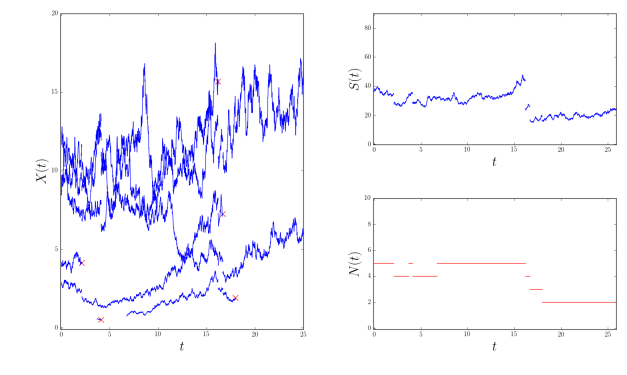
Figure 1. The sample paths of $X,S,N$ with $N(0):=5$, $\sigma:=0.2$, $r:=0.05$. The initial distribution of $\,X\,$ is i.i.d. standard log normal. Default rate is hyperbolic in bank reserves $x$: $\kappa_{n}(s,x)=0.2\cdot n/(0.01+x)$. The contagion measure (default impact) is uniform, i.e., $\mathcal{D}_{n,s,x}\sim\operatorname{Uni}[0,n^{-1}]$, the birth rate is constant $\lambda_{n}(s)=1$, and the new bank distribution is $\mathcal{B}_{n,s}\sim\operatorname{Exp}(1)$ for every $n$ and $s$. The $\times$ markers in the left panel represent defaults.

3. Existence and Stability

3.1. Conditions for existence

The following two lemmas describe the elementary properties of the Markov transition kernel of $X$. First, the process $X$ is totally irreducible. That is, its transition kernel $P^{t}(\mathbf{x},\cdot)$ is positive with respect to the Lebesgue measure $\operatorname{\bm{\mu}}$ on $\mathcal{X}$.

Lemma 1.

For all Borel subsets $A\subseteq\mathcal{X}$ with $\operatorname{\bm{\mu}}(A)>0$, we have:

(3.1) $$P^{t}(\mathbf{x},A):=\mathbb{P}(X(t)\in A\,|\,X(0)=\mathbf{x})>0\quad\mbox{for all}\quad t>0,\,\mathbf{x}\in\mathcal{X}.$$

This positivity property is used for the stability of $X$. The proof of Lemma 1 is in Section 6.4.

Second, due to local boundedness of the intensities of birth and default, $X$ satisfies the Feller property. The following Lemma follows from construction of $X$ by patching: constructing the continuous parts jump-after-jump; see [Bas79, Saw70].

Lemma 2.

The process $X$ is Feller continuous: That is, for any bounded continuous function $f:\mathcal{X}\to\mathbb{R}$, with convention that $f(\Delta)=0$, where $\Delta$ is the (isolated) cemetery state, the function $P^{t}f$ is also bounded and continuous for every $t>0$.

We proceed to state some sufficient conditions when $X$ is conservative, i.e., well-defined on the infinite time horizon so that $\tau_{\infty}=\infty$ a.s. We sometimes say in this case that the system does not explode. To this end, it suffices to find a Lyapunov function. This is a standard tool to prove that a random process is conservative or stable: See for example classic papers [MT93a, MT93b, DMT95]. Essentially, for our proof that $X$ is conservative, we need a function $V:\mathcal{X}\to[0,\infty)$ such that:

(a) for every $c>0$ the set $\{\mathbf{x}\in\mathcal{X}\mid V(\mathbf{x})\leq c\}$ is compact (informally “$V(\infty)=\infty$”);

(b) $V\in C^{2}(\mathcal{X})$, and for some constants $k,c>0$, $\mathfrak{L}V(\mathbf{x})\leq kV(\mathbf{x})+c$ for all $\mathbf{x}\in\mathcal{X}$.

For our setting, let us take the following Lyapunov function:

(3.2) $$V_{0}(\mathbf{x}):=\mathfrak{s}(\mathbf{x})+\mathfrak{n}(\mathbf{x}),\quad\mathbf{x}\in\mathcal{X}.$$

This function trivially belongs to $C^{2}(\mathcal{X})$. By construction of the topology on $\mathcal{X}$, the function $V_{0}$ from (3.2) satisfies the property (a) above. Plugging  (3.2) in  (2.10), we get after calculations (recall that $\overline{\mathcal{B}}$ and $\overline{\mathcal{D}}$ are the means of the respective distributions):

(3.3) $$\begin{split}\varphi(\mathbf{x})&:=\mathfrak{L}V_{0}(\mathbf{x})=r\mathfrak{s}(\mathbf{x})+\lambda_{\mathfrak{n}(\mathbf{x})}(\mathfrak{s}(\mathbf{x}))\left[\overline{\mathcal{B}}(\mathfrak{n}(\mathbf{x}),\mathfrak{s}(\mathbf{x}))+1\right]\\ &\qquad\qquad\qquad{}-\sum_{j=1}^{\mathfrak{n}(\mathbf{x})}\kappa_{\mathfrak{n}(\mathbf{x})}(\mathfrak{s}(\mathbf{x}),x_{j})\left[\overline{\mathcal{D}}(\mathfrak{n}(\mathbf{x}),\mathfrak{s}(\mathbf{x}),x_{i})\mathfrak{s}(\mathbf{x})+1\right]\\ &\qquad\qquad\qquad{}-\sum_{i=1}^{\mathfrak{n}(\mathbf{x})}x_{i}\kappa_{\mathfrak{n}(\mathbf{x})}(\mathfrak{s}(\mathbf{x}),x_{i})\left(1-\overline{\mathcal{D}}(\mathfrak{n}(\mathbf{x}),\mathfrak{s}(\mathbf{x}),x_{i})\right).\end{split}$$

Under some assumption on this function $\varphi(\cdot)$, we claim the following. Its proof is in Section 6.5.

Theorem 3.

Assume there exist positive constants $c_{1},c_{2},c_{3}$ such that $\varphi(\cdot)$ in (3.3) satisfies

$$\varphi(\mathbf{x})\leq c_{1}\mathfrak{s}(\mathbf{x})+c_{2}\mathfrak{n}(\mathbf{x})+c_{3}\quad\mbox{for}\quad\mathbf{x}\in\mathcal{X}.$$

Then the system exists and is conservative: It does not explode.

Example 4.

The simplest conservative example is described when the birth $\lambda$ and default rates $\kappa$ are independent of $N(t)$ and $S(t)$. Then the number $N(t)$ of banks at time $t$ forms a birth-death process with birth intensity $\lambda$ and death intensity $\kappa N(t)$. Hence, we can apply the usual sufficient conditions for this process being conservative. If this process is conservative, then the whole system is also conservative, since on each level $\{\mathfrak{n}(\mathbf{x})=N\}$ (for a given number $N$ of banks), the system behaves as a collection of independent geometric Brownian motions.

3.2. Stability of the system

On a macro-level, to obtain stability we need some balance between births and defaults. Recall that A probability measure $\Pi$ on $\mathcal{X}$ is called a stationary distribution or invariant measure for the system above if the following holds: If we start $X(0)\sim\Pi$, then for all $t\geq 0$, we remain at $X(t)\sim\Pi$. The system is called stable if it is nonexplosive, there exists a unique stationary distribution $\Pi$, and for every given initial condition $X(0)\in\mathcal{X}$, the distribution of $X(t)$ converges to $\Pi$ as $t\to\infty$ in the total variation distance:

(3.4) $$\lim\limits_{t\to\infty}\sup\limits_{A\subseteq\mathcal{X}}\left|\mathbb{P}(X(t)\in A)-\Pi(A)\right|=0.$$

Theorem 5.

The system is stable if the set $\{\mathbf{x}\in\mathcal{X}\mid\varphi(\mathbf{x})>-\varepsilon\}$ is compact for some $\varepsilon>0$, i.e., the function $\varphi$ from (3.3) satisfies $\varlimsup_{\mathbf{x}\to\infty}\varphi(\mathbf{x})<0$.

This result immediately follows from [MT93a, MT93b] and Lemmata 1, 2, [Sar17, Proposition 2.2, Lemma 2.3]. From the definition of compactness in $\mathcal{X}$ from Section 2, there exist constants $\varphi_{0},s_{0},N_{0}>0$ such that $\varphi(\mathbf{x})\leq-\varphi_{0}$ for $\mathfrak{s}(\mathbf{x})\geq s_{0}$ or $\mathfrak{n}(\mathbf{x})\geq N_{0}$.

Example 6.

A simple condition for stability is to have banks with finite lifetime, i.e., the default time $\tau_{i}$ of any bank $i$ is finite a.s. In that case the system will be stable as long as the birth rate remains bounded. Assume $\mathcal{B}_{n,s}$ and $\mathcal{D}_{n,s,x}$ depend only on $n$, and

$$\lambda_{*}:=\sup\limits_{n}\frac{1}{n}\lambda_{n}(s)<\infty,\ \mbox{and}\ \kappa_{n}(s,x_{i})\equiv g(x_{i}),$$

for some decreasing function $g:(0,\infty)\to\mathbb{R}_{+}$, with $g(0+)=+\infty$ and $g(+\infty)=:\kappa_{*}>0$. Then each bank has finite lifetime, which is dominated from above by an exponential random variable with rate $\kappa_{*}$. Therefore, the quantity of banks is stochastically dominated by a birth-death process with birth intensities $\lambda_{*}n$ and death intensities $\kappa_{*}n$ at level $n\geq 1$. If $\kappa_{*}>\lambda_{*}$ then this birth-death process is stable. Combining this observation with the independence of $\mathcal{B}_{n,s}$ and $\mathcal{D}_{n,s,x}$ of $x$ and $s$, we get that the whole system $X$ is stable.

3.3. Refinements of stability results

A stronger convergence than (3.4) (in the total variation distance from (2.7)) can happen exponentially fast as $t$ grows: There exist positive constants $C$ (depending on the initial condition $X(0)$) and $\alpha$ such that

(3.5) $$\sup\limits_{A\subseteq\mathcal{X}}\left|\mathbb{P}(X(t)\in A)-\Pi(A)\right|\leq Ce^{-\alpha t}.$$

Theorem 7.

The system $X$ satisfies (3.5) if there exist constants $c_{1},c_{2},c_{3}>0$ such that

(3.6) $$\varphi(\mathbf{x})\leq-c_{1}\mathfrak{s}(\mathbf{x})-c_{2}\mathfrak{n}(\mathbf{x})+c_{3},\quad\mathbf{x}\in\mathcal{X},$$

where $\varphi(\mathbf{x})$ is defined in (3.3). More generally, the system satisfies a stronger convergence statement: For the function $V_{0}$ defined in (3.2), there exist positive constants $C$ and $\alpha$ such that for all $\mathbf{x}\in\mathcal{X}$, the transition function $P^{t}(\mathbf{x},\cdot)$ of the Markov process $X$ satisfies

(3.7) $$\left\lVert P^{t}(\mathbf{x},\cdot)-\Pi(\cdot)\right\rVert_{V_{0}}\leq CV_{0}(\mathbf{x})e^{-\alpha t}.$$

Example 8.

Assume the following parameters do not depend on $n$, $x$, and $s$:

$$\lambda_{n}(s)\equiv\lambda,\quad\kappa_{n}(s,x)\equiv\kappa,\quad\overline{\mathcal{B}}(n,s)\equiv\overline{\mathcal{B}},\quad\overline{\mathcal{D}}(n,s,x)\equiv\overline{\mathcal{D}}$$

with some constants $\lambda,\kappa,\overline{\mathcal{B}},\overline{\mathcal{D}}>0$. Then the function $\varphi$ from (3.3) becomes

$$\varphi(\mathbf{x})=r\mathfrak{s}(\mathbf{x})+\left[\overline{\mathcal{B}}+1\right]\lambda-\overline{\mathcal{D}}\kappa\cdot\mathfrak{s}(\mathbf{x})\mathfrak{n}(\mathbf{x})-\kappa\mathfrak{n}(\mathbf{x})-\kappa(1-\overline{\mathcal{D}})\cdot\mathfrak{s}(\mathbf{x}).$$

Since $\mathfrak{n}(\mathbf{x})\geq 1$ for $\mathbf{x}\in\mathcal{X}\setminus\{0\}$, the condition of Theorem 5 holds when $\kappa(1-\overline{\mathcal{D}})>r$; that is, when the intensity of defaults, adjusted by the average contagion effect exceeds the growth rate of non-defaulting bank reserves.

Finally, we can sometimes find an explicit estimate for the rate $\alpha$ of exponential convergence. This is done using the coupling argument from [LMT96, Sar16, IS].

Theorem 9.

Assume $\lambda_{n}(y)\leq\lambda^{*}_{n}$ and $\kappa_{n}(y,x)\geq\kappa^{*}_{n}$ for all $n,x,y$. Take a nondecreasing function $\hat{V}:\{0,1,2,\ldots\}\to[1,\infty)$ such that $\hat{V}(0)=1$, and

(3.8) $$\lambda^{*}_{n}\hat{V}(n+1)+n\kappa^{*}_{n}\hat{V}(n-1)-(\lambda^{*}_{n}+n\kappa^{*}_{n})\hat{V}(n)\leq-\alpha V(n),\quad n=1,2,\ldots$$

Define $\tilde{V}:\mathcal{X}\to[1,\infty)$ via $\tilde{V}(\mathbf{x}):=\hat{V}(\mathfrak{n}(\mathbf{x}))$. (The function $\tilde{V}$ depends only on the quantity of components in the vector $\mathbf{x}$.) Then there exists a positive constant $C$ such that

$$\left\lVert P^{t}(\mathbf{x},\cdot)-\Pi(\cdot)\right\rVert_{\operatorname{TV}}\leq C\tilde{V}(\mathbf{x})e^{-\alpha t},\quad\mathbf{x}\in\mathcal{X},\quad t\geq 0.$$

Example 10.

Assume $\lambda^{*}_{n}\leq\lambda_{*}<\kappa_{*}\leq\kappa^{*}_{n}$ for constants $\lambda_{*},\,\kappa_{*}$. Then we can take $\hat{V}(n)=n+1$ and $\alpha:=(\kappa_{*}-\lambda_{*})/2$, since the left-hand side of (3.8) is less than or equal to

$$n\lambda_{*}-n\kappa_{*}\leq-2n\alpha\leq-(n+1)\alpha=-\alpha\hat{V}(n),\quad n=1,2,\ldots.$$

4. Large-Scale Behavior: First Setting

To analyze the distribution of bank reserves we consider the following scaling limit as the number of banks tends to infinity. Fix an index $p\geq 2$. Consider a sequence of systems $(X^{(N)})_{N\geq 1}$ governed by the same dynamics as described in Section 2, with the same parameters $\lambda_{\cdot}(\cdot)$, $\mathcal{B}_{\cdot,\cdot}$, $\kappa_{\cdot}(\cdot,\cdot)$ such that $\mathfrak{n}(X^{(N)}(0))=N$: the system $X^{(N)}$ starts with $N$ banks at time $t=0$. With the empirical measure $\mu_{\cdot}$ in (2.1) let us define the empirical measure process

(4.1) $$\mu^{(N)}=\bigl{(}\mu^{(N)}_{t},\,t\geq 0\bigr{)},\quad\mu_{t}^{(N)}:=\mu_{X^{(N)}(t)}.$$

We focus on the current level and current size

$$\mathcal{N}_{N}(t):=\mathfrak{n}\left(X^{(N)}(t)\right)\quad\mbox{and}\quad\mathcal{S}_{N}(t)=\mathfrak{s}\bigl{(}X^{(N)}(t)\bigr{)},\ t\geq 0,$$

of the systems, as well as the current mean reserves:

$$\mathbf{m}_{N}(t):=\frac{\mathcal{S}_{N}(t)}{\mathcal{N}_{N}(t)}=\overline{X^{(N)}(t)}.$$

4.1. McKean-Vlasov jump-diffusions

Now, let us describe the limiting measure-valued process which is a McKean-Vlasov jump-diffusion. This is a generalization of a McKean-Vlasov diffusion (with drift and diffusion coefficients depending not only on the current process, but on its distribution) to a jump-diffusion.

Consider a filtered probability space $(\Omega,\mathfrak{F},(\mathfrak{F}_{t})_{t\geq 0},\mathbb{P})$ with the filtration satisfying the usual conditions, and another measurable space $(\mathcal{U},\mathfrak{U})$ with a finite measure $\mathfrak{n}$. Fix $p>1$. Recall that $\mathcal{P}_{p}$ is the space of probability measures on $\mathbb{R}$ with finite $p$th moment, which is a metric space with respect to the Wasserstein distance $\mathcal{W}_{p}$.

Assume $W=(W(t),\,t\geq 0)$ is an $(\mathfrak{F}_{t})_{t\geq 0}$-Brownian motion, and $\mathbb{N}=(\mathbb{N}(t),\,t\geq 0)$ is an $(\mathfrak{F}_{t})_{t\geq 0}$-Poisson process with intensity $\lambda$, independent of $W$. Fix drift and diffusion functions $g,\sigma:\mathbb{R}\times\mathcal{P}_{p}\to\mathbb{R}$, as well as a $\mathcal{P}_{p}$-valued function $\mu:\mathbb{R}\times\mathcal{P}_{p}\to\mathcal{P}_{p}$ for jump size distributions. Also, fix a positive number $\lambda>0$. A process $Z=(Z(t),\,t\geq 0)$ with paths in the Skorohod space $\mathcal{D}[0,\infty)$ is called a McKean-Vlasov jump-diffusion if it satisfies

(4.2) $$Z(t)=Z(0)+\int^{t}_{0}\left[g(Z(s),\nu(s))\,\mathrm{d}s+\sigma(Z(s),\nu(s))\,\mathrm{d}W(s)\right]+\sum\limits_{k=1}^{\mathbb{N}(t)}\bigtriangleup Z(\tau_{k}),$$

where $0=\tau_{0}<\tau_{1}<\tau_{2}<\ldots$ are the jump times of the Poisson process $\mathbb{N}=(\mathbb{N}(t),\,t\geq 0)$ with intensity $\lambda$, and $\bigtriangleup Z(t)=Z(t)-Z(t-)\sim\mu_{Z(t-),\nu(t-)}$ for $t\geq 0$. Here, $\nu(t)$ is the distribution of $Z(t)$; and $\nu(t-)$ is the weak limit of $\nu(s)$ as $s\uparrow t$ (similarly to $Z(t-)$). Somewhat abusing the notation, we also call $\bm{\nu}$, which is the distribution of the process $Z$, a solution to (4.2).

To give some explanation about the process $Z$: Between jumps it behaves as a continuous McKean-Vlasov nonlinear diffusion, with drift and diffusion coefficients dependent not only on its current state, but also on its current distribution. The jump measure corresponds to killing $Z$ with rate $\lambda$, and restarting it according to the measure $\mu_{Z(t-),\nu(t-)}$ at every jump moment $t$.

We now state an existence and uniqueness result for $\mathcal{W}_{p}$, $p\geq 1$. Its proof is very similar to the result of [Gra92b, Theorem 2.2] for $\mathcal{W}_{1}$. We refer the interested reader also to [Gra92a, Fun84].

Lemma 11.

Fix $p\geq 1$. Assume $g,\sigma$ are jointly Lipschitz (with respect to $\mathcal{W}_{p}$ for their second argument), and $h$ is jointly Lipschitz with respect to the $L^{p}$-norm. That is, there exists a constant $C>0$ such that for all $x_{1},x_{2}\in\mathbb{R}$ and $\zeta_{1},\zeta_{2}\in\mathcal{P}_{p}$, we have:

(4.3) $$\begin{split}|g(x_{1},\zeta_{1})-g(x_{2},\zeta_{2})|&\leq C\left(|x_{1}-x_{2}|+W_{p}(\zeta_{1},\zeta_{2})\right),\\ |\sigma(x_{1},\zeta_{1})-\sigma(x_{2},\zeta_{2})|&\leq C\left(|x_{1}-x_{2}|+W_{p}(\zeta_{1},\zeta_{2})\right),\\ W_{p}\left(\mu_{x_{1},\zeta_{1}},\mu_{x_{2},\zeta_{2}}\right)&\leq C\left(|x_{1}-x_{2}|+W_{p}(\zeta_{1},\zeta_{2})\right).\end{split}$$

Take an initial condition $Z(0)\sim\nu(0)\in\mathcal{P}_{p}$. Then the equation (4.2) has a unique solution, which is an element of $\mathcal{P}_{p}(\mathcal{D}[0,T])$ for every $T>0$.

Remark 12.

Note that within this framework it is possible to accommodate varying intensity of jumps, that is, $\lambda$ dependent on $Z(t)$ and $\nu(t)$. Indeed, assume that $\lambda=\lambda(Z(t),\nu(t))$ is bounded from above by a constant $\overline{\lambda}$. Instead of the measures $\mu_{z,\nu}$, we can consider measures

(4.4) $$\tilde{\mu}_{z,\nu}:=\overline{\lambda}^{-1}\left[\lambda(z,\nu)\mu_{z,\nu}+(\overline{\lambda}-\lambda(z,\nu))\delta_{z}\right]$$

under the assumption that the intensity of jumps is now constant and is equal to $\overline{\lambda}$. If $\lambda(z,\nu)$ is Lipschitz in $z$ and $\nu$, and the third among (4.3) holds for the family $(\mu_{z,\nu})$, then the family $(\tilde{\mu}_{z,\nu})$ of measures from (4.4) also satisfy the third condition in (4.3).

Next, we can prove that the McKean-Vlasov jump-diffusion $\,Z\,$ in (4.2) satisfies for $p\geq 1$

$$\lim_{s\to t}\mathbb{E}[|Z(s)-Z(t)|^{p}]\,=\,0\qquad\forall t\in[0,T].$$

This implies that the mapping $t\mapsto\nu(t)$ is continuous, i.e., $\nu\in C([0,T],\mathcal{W}_{p})$. We can state the McKean-Vlasov-Itô process in an equivalent form as a martingale problem. For a function $f\in\mathcal{C}^{2}_{b}$, a scalar $z\in\mathbb{R}$, and a probability measure $\nu\in\mathcal{P}_{p}$, define

(4.5) $$\mathcal{L}f(z,\nu)=g(z,\nu)f^{\prime}(z)+\frac{1}{2}\sigma^{2}(z,\nu)f^{\prime\prime}(z)+\lambda\int_{\mathbb{R}}\left[f(z+u)-f(z)\right]\mu_{z,\nu}(\mathrm{d}u).$$

We say that a probability measure $\bm{\nu}$ in $\mathcal{P}_{p}(\mathcal{D}[0,T])$ is a solution to a McKean-Vlasov jump-diffusion martingale problem, if for every function $f\in\mathcal{C}^{2}_{b}$ the process

(4.6) $$f(Z(t))-f(Z(0))-\int_{0}^{t}\mathcal{L}f(Z(s),\nu(s))\,\mathrm{d}s,\ t\in[0,T],$$

is a martingale, where $\nu(s)$ is the projection of $\bm{\nu}$ at time $s$, and $Z\sim\bm{\nu}$ is a canonical stochastic process with trajectories in $\mathcal{D}[0,T]$. Taking expectations of this martingale, taking derivatives with respect to time, and then using that $Z(t)\sim\nu(t)$, we arrive at the following ODE

(4.7) $$\frac{\mathrm{d}}{\mathrm{d}t}(\nu(t),f)=(\nu(t),\mathcal{L}f(\cdot,\nu(t))),\quad t\in[0,T].$$

Equation (4.7) characterizes the McKean-Vlasov-Itô equation via martingale problems. The following lemma summarizes our description of McKean-Vlasov jump-diffusions.

Lemma 13.

Under the assumptions of Lemma 11, an adapted process $Z=(Z(t),\,t\geq 0)$ with rcll trajectories, with distribution $\nu(t)\sim Z(t)$, is a McKean-Vlasov jump-diffusion as in (4.2), if and only if for every test function $f\in\mathcal{C}^{2}_{b}$, the process in (4.6) is a martingale; or, equivalently, if for every test function $f\in\mathcal{C}^{2}_{b}$, the equation (4.7) holds.

The proof of Lemma 13 follows standard arguments (see for example [KS91, Section 5.4] or [EK86, Section 4.4]) and is therefore omitted.

Remark 14.

In Section 5 we shall need a version of (4.2) with parameters $g,\,\sigma,\,\mu$, depending not only on $Z(t)$ and $\nu(t)$, but on the whole history $Z(s)\,,\nu(s)\,,0\leq s\leq t$, as well as on time $t$. Thus, this McKean-Vlasov jump-diffusion is path-dependent and time-inhomogeneous. Similar to (4.3) we then modify the Lipschitz conditions as follows: For $t\in[0,T]$, $z_{1},z_{2}\in D[0,t]$, and $\bm{\nu}_{1},\bm{\nu}_{2}\in C([0,t],\mathcal{P}_{p})$, with $\nu_{1}(s)$, $\nu_{2}(s)$ being push-forwards of $\bm{\nu}_{1}$, $\bm{\nu}_{2}$ with respect to the projection mapping $x\mapsto x(s)$ for each $0\leq s\leq t$, we define the distance function:

$$\Delta(t):=\sup\limits_{0\leq s\leq t}|z_{1}(s)-z_{2}(s)|+\sup\limits_{0\leq s\leq t}\mathcal{W}_{p}(\nu_{1}(s),\nu_{2}(s)),$$

and impose the following Lipschitz conditions:

(4.8) $$\begin{split}\left|g(t,z_{1},\bm{\nu}_{1})-g(t,z_{2},\bm{\nu}_{2})\right|&\leq C\cdot\Delta(t),\\ \left|\sigma(t,z_{1},\bm{\nu}_{1})-\sigma(t,z_{2},\bm{\nu}_{2})\right|&\leq C\cdot\Delta(t),\\ \mathcal{W}_{p}\left(\mu_{t,z_{1},\bm{\nu}_{1}},\mu_{t,z_{2},\bm{\nu}_{2}}\right)&\leq C\cdot\Delta(t).\end{split}$$

Then Lemma 11 and Lemma 13 still hold, with the formula for the generator (4.5).

4.2. Mean-field limit: first main result

We investigate the limiting behavior of the empirical measure process $(\mu^{(N)}_{t},\,t\geq 0)$ as $N\to\infty$. We shall show that these measure-valued processes converge, in fact, to a deterministic measure-valued process, governed by a certain McKean-Vlasov equation. To this end, we impose some additional assumptions on the parameters of our model as the number of banks $n$ tends to infinity. Note that in our scaling, we re-parametrize in terms of $n$ and $y=s/n$ (i.e., $s=ny$) in reference to the mean size $\mathbf{m}$ above.

Assumption 15.

As $n\to\infty$, $\mathcal{B}_{n,ny}\to\mathcal{B}_{\infty,y}$ in the Wasserstein distance $\mathcal{W}_{p}$, uniformly over $y>0$, with the family $(\mathcal{B}_{\infty,y})_{y>0}$ continuous in $\mathcal{W}_{p}$; and the measures $\mathcal{B}_{n,s},\,n\geq 0,\,s>0$ have uniformly bounded $p$-th moments.

Assumption 16.

As $n\to\infty$, we assume uniform convergence to a continuous limit $\lambda_{\infty}$:

$$\frac{\lambda_{n}(ny)}{n}\to\lambda_{\infty}(y),\,y>0$$

uniformly in $y>0$. Moreover, there exists a constant $C_{\lambda}$ such that $\lambda_{n}(s)\leq C_{\lambda}(n+s)$ for all $n,s$.

Examples of birth rates satisfying Assumption  16 are $\lambda_{n}(s)=\bar{\lambda}s$ (new banks formed at rate proportional to total reserves) and $\lambda_{n}(s)=\bar{\lambda}n$ (new banks formed at rate proportional to current number) for a constant $\bar{\lambda}>0$, which both lead to $\lambda_{\infty}(y)=\bar{\lambda}y$. Note that birth rates must increase as system size $N$ grows to avoid the trivial limit $\lambda_{\infty}=0$.

Assumption 17.

If $\xi_{n,s,x}\sim\mathcal{D}_{n,s,x}$, then $n\xi_{n,ny,x}\to\xi_{\infty,y,x}\sim\mathcal{D}_{\infty,y,x}$ as $n\to\infty$ in the Wasserstein distance $\mathcal{W}_{p}$ uniformly over all $x,y>0$, where the family of measures $(\mathcal{D}_{\infty,y,x})_{x,y>0}$ is continuous in $\mathcal{W}_{p}$ jointly in $x$ and $y$; support of measures $\mathcal{D}_{\infty,y,x}$ is bounded from above uniformly in $x$ and $y$; and $\xi_{\infty,y,x}$ has uniformly bounded $p$th moment over all $x,y$.

Remark 18.

From (17) it follows that for $q\leq p$,

(4.9) $$C_{\mathcal{D},q}:=\sup\limits_{N,x,s}\bigl{[}N^{q}\int_{0}^{1}z^{q}\,\mathcal{D}_{N,x,s}(\mathrm{d}z)\bigr{]}<\infty,$$

and there exist $n_{0}$ and $\varepsilon_{0}\in(0,1)$ such that a.s. for all $n\geq n_{0}$, $0<x<ny$, $|\xi_{n,y,x}|\leq 1-\varepsilon_{0}$.

The requirement in Assumption 17 is that the default impact decreases inversely proportional to the scaling parameter. Larger banking systems will experience more defaults (namely proportionally to $N$, see the next assumption), so the impact of each default must shrink to compensate. Note that the limiting distribution $\mathcal{D}_{\infty,y,x}$ does not matter and only its mean will appear in the limit equation. An example would be $\xi_{n,s,x}\sim\operatorname{Uni}(0,\bar{d}/n)$ so that $\xi_{\infty,y,x}\sim\operatorname{Uni}(0,\bar{d})$. The next assumption is about the convergence of the default rates. Another example would be the case when default rates are independent of $n,s$: $\kappa_{\infty}(x)=\kappa_{n}(x)$.

Assumption 19.

As $n\to\infty$, uniformly over $y,x\in(0,\infty)$, we have: $\kappa_{n}(ny,x)\to\kappa_{\infty}(y,x)$, with $\kappa_{\infty}(y,x)$ continuous in $y$. Moreover, there exists a constant $C_{\kappa}$ independent of $x$, $n$ and $s$ such that $\kappa_{n}(s,x)\leq C_{\kappa}$ for all $n,s,x$.

Denote the means of the limiting measures $\mathcal{B}_{\infty,y}$ and $\mathcal{D}_{\infty,y,x}$ by $\overline{\mathcal{B}}_{\infty}(y)$ and $\overline{\mathcal{D}}_{\infty}(y,x)$. Define

(4.10) $$\psi(x,y):=r-\overline{\mathcal{D}}_{\infty}(y,x)\kappa_{\infty}(y,x),\qquad y>0,$$

(4.11) $$\mathcal{G}_{y}f(x):=\psi(x,y)D_{1}f(x)+\frac{\sigma^{2}}{2}D_{2}f(x)=\mathcal{G}f(x)-\overline{\mathcal{D}}_{\infty}(x,y)\kappa_{\infty}(x,y)D_{1}f,$$

where $\mathcal{G}$ is from (2.4). This will be the limiting diffusion term, corresponding to the original geometric Brownian motion dynamics, summarized by $\mathcal{G}$ plus the additional mean-field-based drift term due to the default interactions. Define the measure-valued process $\mu^{(\infty)}=(\mu^{(\infty)}_{t},\,t\geq 0)$ as the law of a McKean-Vlasov jump-diffusion with generator

(4.12) $$\begin{split}\mathcal{L}_{\nu}f(z)&:=\mathcal{G}_{\overline{\nu}}f+\lambda_{\infty}\left(\overline{\nu}\right)\int_{0}^{\infty}\left[f(w)-f(z)\right]\,\mathcal{B}_{\infty,\overline{\nu}}(\mathrm{d}w)\\ &+\kappa_{\infty}(\overline{\nu},z)\int_{0}^{\infty}\left[f(w)-f(z)\right]\,\nu(\mathrm{d}w).\end{split}$$

We can apply current distribution $\nu$ to this generator and get:

(4.13) $$\begin{split}\mathcal{A}(\nu,f):=(\nu,\mathcal{L}_{\nu}f)&=(\nu,\mathcal{G}_{\overline{\nu}}f)+\lambda_{\infty}\left(\overline{\nu}\right)\big{[}\left(\mathcal{B}_{\infty,\overline{\nu}},f\right)-\left(\nu,f\right)\big{]}\\ &+(\nu,f)\left(\nu,\kappa_{\infty}\left(\overline{\nu},\cdot\right)\right)-\left(\nu,\kappa_{\infty}\left(\overline{\nu},\cdot\right)f\right).\end{split}$$

The main result below is that $\mu^{(\infty)}$ is a suitable limit of $\mu^{(N)}$’s from (4.1). To explain the form of $\mathcal{A}$ we discuss each term. First, the $\mathcal{G}_{\overline{\nu}}$ term arises from the additional average downward drift from the defaults. Next, there are two different jump mechanisms: The second piece

(4.14) $$\lambda_{\infty}\left(\overline{\nu}\right)\left(\mathcal{B}_{\infty,\overline{\nu}},f\right)-\lambda_{\infty}\left(\overline{\nu}\right)\left(\nu,f\right)$$

arises from births from the pre-limit finite system which translate into killing and restarting according to the measure $\mathcal{B}_{\infty,\cdot}$. This can be viewed as exogenous “regeneration” with a source measure $\mathcal{B}_{\infty,\overline{\nu}}$. The third piece

(4.15) $$(\nu,f)\left(\nu,\kappa_{\infty}\left(\overline{\nu},\cdot\right)\right)-\left(\nu,\kappa_{\infty}\left(\overline{\nu},\cdot\right)f\right)$$

is an endogenous push due to the non-constant default intensity. Regions where $\kappa_{\infty}$ is higher experience higher rates of defaults, whereby the respective banks “dis-appear”; in the limit they immediately “re-appear” according to $\nu$. This can be thought of as a genetic mutation: particles in high-default regions get killed and replaced with new particles sampled according to $\nu$.

If $\kappa_{\infty}(y,x)=\kappa_{\infty}(y)$ depends only on $y$, then the term (4.15) vanishes. Indeed, this term then becomes proportional to the action $(\nu,f)$ of the current distribution $\nu$ on the test function $f$. This means we kill the process and restart it at the same distribution, which is equivalent to doing nothing. Thus, only the decrease of reserves of all remaining banks by i.i.d. fractions influences the empirical measure, turning the drift from $r$ into $\psi$ from (4.10).

Financially, we see that defaults from the pre-limit finite system translate into two effects. On the one hand, defaults themselves create additional downward drift inside $\psi$ from (4.10), as compared with the original drift $r$. On the other hand, financial contagion after a default creates reset times when the process is killed and restarted, which corresponds to the term (4.15). Let us mention how bankruptcies occur in this limit: The fraction of banks defaulting at time $[t,t+\Delta t]$ is $\kappa_{\infty}(\mathbf{m}(t))\,\mathrm{d}t$. That is, the fraction of banks defaulted during time interval $[s,t]$ is $\int_{s}^{t}\kappa_{\infty}(\mathbf{m}(u))\,\mathrm{d}u$. This fraction can be greater than $1$, because new banks emerge all the time.

In the notation of (4.2), we interpret the mean field limit as a McKean-Vlasov jump-diffusion $Z$ which has drift $\psi(Z(t),\nu_{t})Z(t)$, diffusion $\sigma Z(t)$ and the following family of jump measures:

(4.16) $$\mu_{z,\nu}(\mathrm{d}w)=\lambda_{\infty}\left(\overline{\nu}\right)\,\mathcal{B}_{\infty,\overline{\nu}}(\mathrm{d}w)+\kappa_{\infty}(\overline{\nu},z)\,\nu(\mathrm{d}w).$$

The process $Z$ can be thought of as a ‘representative particle’.

Lemma 20.

Under Assumptions  15, 16, 17, 19, there exists a unique McKean-Vlasov jump-diffusion $Z$ with generator (4.13).

Proof.

We verify the conditions of Lemma 11. Both terms in (4.16):

$$\lambda_{\infty}\left(\overline{\nu}\right)\mathcal{B}_{\infty,\overline{\nu}}(\mathrm{d}w)\quad\mbox{and}\ \quad\kappa_{\infty}(z,\overline{\nu})\,\nu(\mathrm{d}w)$$

have the $p$th moment uniformly bounded for $p\geq 2$. Note the Lipschitz property of these measures with respect to the measure $\nu$ in $\mathcal{W}_{p}$. Together with the Lipschitz property of the functions $x\mapsto\psi(x,y)x$ and $x\mapsto\sigma x$, this completes the proof. ∎

The following is the main result of this section, with proof postponed to Section 7.

Theorem 21.

Suppose the initial empirical measures converge in $\mathcal{W}_{p}$ with $p>1$:

$$\mu^{(N)}_{0}\Rightarrow\mu^{(\infty)}_{0}\ \mbox{as}\ N\to\infty.$$

Under Assumptions 15, 16, 17, 19, we have the following convergence in law in the Skorohod space $\mathcal{D}([0,T],\mathcal{P}_{q})$, for every $T>0$ and $q\in(1,p)$:

$$\mu^{(N)}\Rightarrow\mu^{(\infty)}\ \mbox{as}\ N\to\infty.$$

By Lemma 33, the functional $\nu\mapsto\overline{\nu}$ (taking the mean) is continuous in $\mathcal{P}_{q}$. Thus we have:

Corollary 22.

As $N\to\infty$, we have weak convergence in $\mathcal{D}[0,T]$:

$$\mathbf{m}_{N}(\cdot)\Rightarrow\mathbf{m}(\cdot)\quad\mbox{where}\quad\mathbf{m}(t):=\mathbb{E}[Z(t)]=(\mu^{(\infty)}_{t},f_{1}),$$

4.3. Default intensity independent of size

Under Assumptions 15, 16, 17, 19, if the killing rate and the mean of the contagion measure

$$\kappa_{\infty}(y,x)=\kappa_{\infty}(y)\quad\mbox{and}\quad\overline{\mathcal{D}}_{\infty}(y,x)\,=\,\overline{\mathcal{D}}_{\infty}(y)$$

are independent of the individual size $x$ but dependent only on the average of the system, we can solve the McKean-Vlasov equation explicitly. Indeed, in this case, in the limit $N\to\infty$ default intensities and default impacts are independent of the size of defaulting banks. In this case, we can rewrite (4.10) as $\psi(x,y)=\psi(y)=r-\overline{\mathcal{D}}_{\infty}(y)\kappa_{\infty}(y)$. Then we rewrite the McKean-Vlasov equation for $\mu^{(\infty)}$ as follows:

(4.17) $$Z(t)=Z(0)+\int_{0}^{t}\left[\psi(\mathbf{m}(s))\,Z(s)\,\mathrm{d}s+\sigma Z(s)\,\mathrm{d}B(s)\right]+\sum\limits_{k=1}^{\mathbb{N}(t)}\Delta Z(\tau_{k}),\quad\,\mathbf{m}(t)=\mathbb{E}[Z(t)],$$

with $B=(B(t),\,t\geq 0)$ being a Brownian motion; $\mathbb{N}(t)$ is a time-nonhomogeneous Poisson process with rate $\lambda_{\infty}(\mathbf{m}(t))$, with jump times $\tau_{k}$, and $Z(\tau_{k})\sim\mathcal{B}_{\infty,\mathbf{m}(\tau_{k}-)}$. Assuming the function $\psi$ is Lipschitz continuous, equation (4.17) has a unique solution for any initial condition, see for example [Fun84]. Let us now solve (4.17). Its parameters: drift, volatility, and jump measure $\lambda_{\infty}(\cdot)\mathcal{B}_{\infty,\cdot}$, depend on the distribution of $Z(t)$ only through its mean $\mathbf{m}(t)$. Therefore, we can solve first for $\mathbf{m}(\cdot)$ and then for $Z(t)$. Take expectations in (4.17):

(4.18) $$\mathbf{m}^{\prime}(t)=\psi(\mathbf{m}(t))\mathbf{m}(t)+\lambda_{\infty}(\mathbf{m}(t))\left(\overline{\mathcal{B}}_{\infty}(\mathbf{m}(t))-\mathbf{m}(t)\right),\quad\mathbf{m}(0)=\int_{0}^{\infty}x\mu^{(\infty)}_{0}(\mathrm{d}x).$$

Assuming this (deterministic) ODE has a unique solution $\mathbf{m}(\cdot)$ we plug it in (4.17) to obtain that $Z$ is a geometric Brownian motion with time-dependent drift:

(4.19) $$Z(t)=Z(0)\exp\left[\int_{0}^{t}\left[\psi(\mathbf{m}(s))-\sigma^{2}/2\right]\,\mathrm{d}s+\sigma B(t)\right],$$

killed at rate $\lambda_{\infty}(\mathbf{m}(t))$, and resurrected according to $\mathcal{B}_{\infty,\mathbf{m}(t)}$. Let us find constant solutions $\mu^{(\infty)}_{t}\equiv\Pi$, or, equivalently, stationary solutions for the process $Z$ in (4.19). For any such solution, its mean $\mathbf{m}(t)\equiv M$ is also independent of $t$. Therefore, we let the right-hand side of the ODE (4.18) to be equal to zero. This is an algebraic equation:

(4.20) $$\psi(M)M+\lambda_{\infty}(M)\left(\overline{\mathcal{B}}_{\infty}(M)-M\right)=0.$$

For every solution $M>0$ of this equation (which is notably independent of $\sigma$), from (4.19) we get geometric Brownian motion:

$$\mathrm{d}Z(t)=Z(t)\left[\psi(M)\,\mathrm{d}t+\sigma\,\mathrm{d}B(t)\right],$$

killed at constant rate $\lambda_{\infty}(M)$, and resurrected according to the probability measure $\mathcal{B}_{\infty,M}$. The most elementary case is when all limiting parameters are constant:

(4.21) $$\lambda_{\infty},\,\kappa_{\infty},\,\overline{\mathcal{B}}_{\infty},\,\overline{\mathcal{D}}_{\infty}.$$

Then the differential equation (4.18) takes the form

$$\mathbf{m}^{\prime}(t)=\lambda_{\infty}\overline{\mathcal{B}}_{\infty}+\gamma\mathbf{m}(t),\quad\text{ where }\quad\gamma:=\left(r-\overline{\mathcal{D}}_{\infty}\kappa_{\infty}-\lambda_{\infty}\right).$$

Given the initial condition $\mathbf{m}(0)$, the solution of this first-order linear equation is

(4.22) $$\mathbf{m}(t)=\left(\mathbf{m}(0)-\frac{\lambda_{\infty}\overline{\mathcal{B}}_{\infty}}{\gamma}\right)e^{-\gamma t}+\frac{\lambda_{\infty}\overline{\mathcal{B}}_{\infty}}{\gamma}.$$

If $\gamma\neq 0$, there exists a unique solution to the algebraic equation (4.20), which is the limit for the solution $\mathbf{m}(t)$ of the differential equation (4.22): $M=\gamma^{-1}\lambda_{\infty}\overline{\mathcal{B}}_{\infty}=\lim_{t\to\infty}\mathbf{m}(t)$. The left panel of Figure 2 illustrates the mean field limit in the constant default intensity case. We take $\lambda_{n}(s)=0.2n,\kappa_{n}(s,x)=0.1$, $\mathcal{B}_{n,s}\sim\operatorname{Exp}(1)$ and $\mathcal{D}_{n,s,x}\sim\operatorname{Uni}(0,n^{-1})$, and $r=0.05$. Note that in the mean field limit $\lambda_{\infty}=0.2$, $\kappa_{\infty}(x)=1$ and $\overline{\mathcal{B}}_{\infty}=1,\overline{\mathcal{D}}_{\infty}=0.5$, leading to

$$M=\frac{0.2\cdot 1}{0.2+0.1\cdot 0.5-0.05}=1.$$

In Figure 2 we initialize with $\mu_{0}^{(N)}\sim\operatorname{Exp}(0.5)$ so that $\mathbf{m}(0)=2$ and the solution of (4.22) reads as $\mathbf{m}(t)=1\exp(-0.2t)+1$. The figure shows the simulated distribution of $\mathbf{m}(t)$ based on running 100 paths of the pre-limit system $X^{(N)}$ with $N=5,25,100$. For each run $i=1,\ldots,100$ we compute the resulting $m^{i}_{N}(t)$ as the empirical average bank size at step $t$ and finally plot $\operatorname{Ave}(m^{i}_{N}(t))$, as well as the $5\%-95\%$ quantiles of $m^{i}_{N}(t)$ across the $100$ runs. The latter visualize the variance of $m_{N}(t)$; as expected as $N$ increases, $m_{N}(t)$ converges in distribution to the deterministic limit $\mathbf{m}(t)$ reported above. We note that in this example due to the limited interaction among the banks and the light-tailed default and birth distributions, the convergence is very rapid so already $\mathbb{E}[m_{N}(t)]\simeq\mathbf{m}(t)$ even for very small $N=5$.

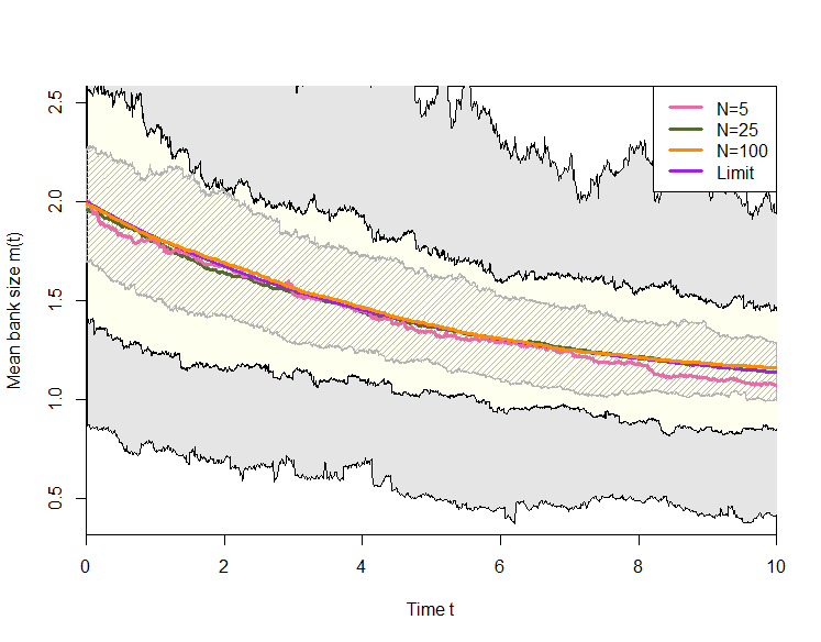
Figure 2. Left panel: distribution of $m_{N}(t)$ on $t\in[0,10]$ and $N=5,25,100$ based on $100$ simulated trajectories of $X^{(N)}$. The initial distribution is $\mu^{(N)}_{0}\sim\operatorname{Exp}(0.5)$ so that $m_{N}(0)=2$. Right panel: distribution of $d_{N}:=(\mu^{(N)}_{T},1_{[0,D]})$, proportion of banks with reserves less than $D=1$ at $T=10$.

4.4. Capital distribution

The mean field limit offers insight into the bank reserves distribution which is key to analyzing the probability of systemic events: when many banks default or have low reserves. For example, in structural models there is typically a risk threshold $D>0$ so that banks whose reserves are below $D$ are viewed as insufficiently capitalized. Taking $f_{D}(x):=1_{\{x\leq D\}}$, the systemic risk of the banking network at epoch $t$ can be assessed as

(4.23) $$\frac{|\#\{i\in I(t)\mid X_{i}(t)\leq D\}|}{N(t)}=\bigl{(}\mu_{t}^{(N)},f_{D}\bigr{)}.$$

As $N\to\infty$, empirical measures $\mu^{(N)}_{t}$ converge in $\mathcal{P}_{q}$ (and therefore weakly) to a deterministic measure $\mu^{(\infty)}_{t}$, which is absolutely continuous and hence $(\mu^{(N)},f_{D})\to\mu^{(\infty)}_{t}(0,D)$. At the same time, as $t$ becomes large, $\mu^{(\infty)}_{t}$ converges to its stationary distribution $\Pi$, so the fraction of banks below $D$ approaches $\Pi(0,D]$.

The right panel of Figure 2 shows the distribution of $d_{N}:=(\mu^{(N)}_{t},f_{D})$ at fixed $t$ as we vary $N$. Specifically, we use the same setting as in the left panel of that Figure and take $D=1$. As expected, $(\mu^{(N)}_{t},f_{D})$ becomes more deterministic as $N$ grows and the empirical fluctuations decrease. In the Figure, we see that about 60% of the banks will have assets below $D=1$ at $T=10$. The take-home message is that analysis of $\Pi$ (and $\mu^{(\infty)}_{\cdot}$ for shorter-term objectives) holds the key for understanding the financial riskiness of the system, for example whether the banks tend to cluster into distinct groups (small banks, large banks, etc.)

4.5. Propagation of chaos

Let us further describe the behavior of a typical bank as the number of banks tends to infinity. Consider, for example, the first bank $X_{1}$ starting from time $t=0$.

Theorem 23.

Assume $X_{1}^{(N)}(0)$ is deterministic for every $N\geq 1$, and $X_{1}^{(N)}(0)\to x_{1}$ as $N\to\infty$. As $N\to\infty$, $X_{1}^{(N)}\Rightarrow X_{1}^{(\infty)}$ weakly in $\mathcal{D}[0,T]$, where $X_{1}^{(\infty)}$ is a solution to the following stochastic differential equation:

(4.24) $$\mathrm{d}X_{1}^{(\infty)}(t)=\psi\bigl{(}X_{1}^{(\infty)}(t),\mathbf{m}(t)\bigr{)}\,X_{1}^{(\infty)}(t)\,\mathrm{d}t+\sigma X_{1}^{(\infty)}(t)\,\mathrm{d}W(t),$$

starting from $x_{1}$, killed with rate $\kappa_{\infty}(\mathbf{m}(t),X_{1}^{(\infty)}(t))$.

The proof of Theorem 23 is in Section 9. Observe that compared to (4.2), the limiting dynamics of $X_{1}$ are simpler: there is still a mean-field interaction through $\mathbf{m}(t)$, but solely via a mean-field killing rate. Births and hence jumps disappear. We can state this result as follows, recalling the definition of the generator (4.11): (4.24) is a McKean-Vlasov diffusion with generator

(4.25) $$\mathcal{A}^{*}_{\nu}f(x_{1})=\mathcal{G}_{\overline{\nu}}f(x_{1})-\kappa_{\infty}\left(\overline{\nu},x_{1}\right)f(x_{1}).$$

Similarly to Theorem 23, we have propagation of chaos. Namely, consider the first $k$ banks instead of only the first one: $(X_{1}^{(N)},\ldots,X_{k}^{(N)}).$ One can show that the resulting limit in $\mathcal{D}([0,T],\mathbb{R}^{k})$ as $N\to\infty$ is a vector of $k$ independent copies of the killed geometric Brownian motion described above: Dependence between the banks vanishes in the limit.

Financially, propagation of chaos offers two convenient features: (1) it abstracts away the complex bilateral dependencies that may exist between individual banks; (2) it distinguishes clearly between the global recurrent nature of the banking system and the individual banks that have finite lifetime (assuming suitable conditions on $\kappa_{\infty}$ which are expected to hold in realistic settings). The latter is the major difference between a representative particle $Z$ that is infinite-lived, and the prototypical bank $X_{1}$ that lives for some time and eventually defaults.

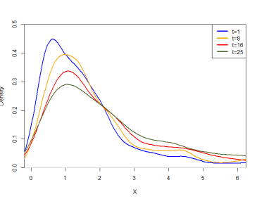
Figure 3. Density of $\nu_{t}$ approximated through an empirical distribution of $\check{X}$ of size $N^{\prime}=500$ (smoothed via built-in kernel density estimator in MATLAB) at $t=1,8,16,25$, with parameters inherited from Figure 1. The initial condition $\nu_{0}$ has the law of $e^{Z}$ for $Z\sim\mathcal{N}(0,1)$ with time step $\Delta t=10^{-3}$.

4.6. Illustrating the McKean-Vlasov equation

The limiting McKean-Vlasov equation can be studied using Monte Carlo approximation. Namely, the measures $\mu^{(\infty)}_{t}$ can be approximated through an empirical distribution of a system $\check{X}$ of $N^{\prime}$ interacting particles. The particles follow the dynamics of the dummy $\{Z(t)\}$, i.e., behave like geometric Brownian motions that are killed and restarted. Note that in contrast to the pre-limit systems $X^{(N)}$, $\check{X}$ has a fixed dimension, $\mathfrak{n}(\check{X}(t))=N^{\prime}\,$ for every $t$. Thus, its dynamics are only in terms of the empirical mean $\check{m}(t):=\frac{1}{N^{\prime}}\sum_{i=1}^{N^{\prime}}\check{X}^{(i)}(t)$, rather than system size $N$ and sum $S$. In turn, we may simulate $\check{X}$ using standard tools, for example an Euler scheme with a fixed time-step $\Delta t$.

To do so, each particle $\check{X}^{(i)}$ follows on $[t,t+\Delta t]$ the geometric Brownian motion dynamics with drift $\psi(\check{X}^{(i)}(t),\check{m}(t))$ and volatility $\sigma$, driven by independent Brownian motions $\check{W}_{i}(\cdot)$. In addition, each particle carries two exponential clocks that fire off at rates $\lambda_{\infty}(\check{m}(t))$ and $\kappa_{\infty}(\check{m}(t),\check{X}^{(i)}(t))$ respectively. Alarms of the first type result in regeneration, i.e., the respective particle instantaneously jumps from its current location $\check{X}^{(i)}(t-)$ to a location $\zeta\sim\mathcal{B}_{\infty,\check{m}(t)}$, generated independently of everything else. Alarms of the second type result in resampling due to non-uniform default rates: the particle jumps from $\check{X}^{(i)}(t-)$ to the location of another particle $j$, $\check{X}^{(i)}(t)=\check{X}^{(j)}(t)$, with index $j$ sampled uniformly from $\{1,2,\ldots,i-1,i+1,\ldots,N^{\prime}\}$. After this mutation procedure, which can be interpreted as killing particle $i$ and replacing it with a child of particle $j$, the two “sibling” particles resume independent movements as geometric Brownian motions.

Figure 3 shows the distribution of the McKean-Vlasov solution: the density $\nu_{t}$ (which has no closed-form expression) for several values of $t$ with the state-dependent default rates. We take limits of parameters from Figure 1. That is,

$$\lambda_{\infty}(y)=1,\quad\mathcal{B}_{\infty,y}\sim\operatorname{Exp}(1),\quad\kappa_{\infty}(y,x)=\frac{0.2}{0.01+x},\quad\mathcal{D}_{\infty,y,x}\sim\operatorname{Uni}[0,1].$$

5. Large-Scale Behavior: Second Setting

For a systemic risk application, our main interest is to build a model with a stationary $\{N(t)\}$. Indeed, we wish to have a dynamic banking network that expands and shrinks over time but is globally infinite-lived, even if individual banks have finite lifetimes. However, observe that in the setup above, asymptotically both the birth rate $\lambda_{n}(s)$ and the aggregate default rate $n\cdot\kappa_{n}(s,x)$ are linear in $n$. Thus they are comparable, and either births or defaults will ultimately dominate, so that the number of banks $N(t)$ will exponentially grow/shrink in $t$. In other words, starting with a finite $N(0)$, $\mathbb{E}[N(t)]$ will then either exponentially grow to $+\infty$ or exponentially collapse to $0$, neither of which are financially plausible.

To circumvent this issue (which is ultimately not important in the mean-field limit), in this section we consider the case when all parameters of the $N$th system, with $N$ the initial number of banks, are independent of $n$, the current number of banks, but depend on the initial $N$. The motivation is to have models with constant birth rates, whereby $\{N(t)\}$ roughly behaves as a linear birth-and-death process with the classical Poisson stationary distribution. We then again scale the systems to recover a (different!) McKean-Vlasov limit. This setting also intrinsically ensures the global recurrence.

To do so, we need to adjust Assumptions 15, 16, 17, 19, accordingly. Everywhere instead of subscript $n$ we now write $N$, because we now index parameters by the initial size $N$. Consider a sequence $(X^{(N)})_{N\geq 1}$ of banking systems with the initial values $X^{(N)}(0)=x^{(N)}_{0}\in\mathbb{R}^{N},\quad\mathfrak{n}(x^{(N)}_{0})=N$. The $N$th system $X^{(N)}$ is governed by birth intensities $\lambda_{N,n}(ny)=\lambda_{N}(y)$, birth measures $\mathcal{B}_{N,n,ny}=\mathcal{B}_{N,y}$, default intensities $\kappa_{N,n}(ny,x)=\kappa_{N}(y,x)$, and default contagion measures $\mathcal{D}_{N,n,ny,x}=\mathcal{D}_{N,y,x}$. In all these assumptions, we abuse the notation by dropping the dependence on $n$ (there is now only indirect dependence through $y=s/n$, the mean of the system).

Assumption 24.

As $N\to\infty$, $\mathcal{B}_{N,y}\to\mathcal{B}_{\infty,y}$ in the Wasserstein distance $\mathcal{W}_{p}$, uniformly over $y>0$, with the family $(\mathcal{B}_{\infty,y})_{y>0}$ continuous in $\mathcal{W}_{p}$; and the measures $\mathcal{B}_{N,y}$ have uniformly bounded $p$-th moments for all $N,y$.

Assumption 25.

As $N\to\infty$, we assume uniform convergence to a continuous limit $\lambda_{\infty}$:

$$\frac{\lambda_{N}(y)}{N}\to\lambda_{\infty}(y),\,y>0$$

uniformly in $y>0$; and for some constant $C_{\lambda}$, we have $\lambda_{N}(y)\leq C_{\lambda}(N+y)$ for all $N,y$.

Assumption 26.

If $\xi_{N,y,x}\sim\mathcal{D}_{N,y,x}$, then $N\xi_{N,y,x}\to\xi_{\infty,y,x}$ as $N\to\infty$ in the Wasserstein distance $\mathcal{W}_{p}$ uniformly over all $x,y>0$, where the family of measures $(\xi_{\infty,y,x})_{x,y>0}$ is continuous in $\mathcal{W}_{p}$ jointly in $x$ and $y$; and $N\xi_{N,y,x}$ has uniformly bounded $p$th moment over all $N,x,y$. We denote the corresponding limiting measure by $\mathcal{D}_{\infty,y,x}$.

Assumption 27.

As $N\to\infty$, uniformly over $y,x\in(0,\infty)$, we have: $\kappa_{N}(y,x)\to\kappa_{\infty}(y,x)$, with $\kappa_{\infty}(y,x)$ continuous in $y$. Moreover, there exists a constant $C_{\kappa}$ independent of $x,y,N$ such that $\kappa_{N}(y,x)\leq C_{\kappa}$ for all $N,x,y$.

Example 28.

Continuing the example from Figure 2, we take $\lambda_{N}(s)=\bar{\lambda}N=0.2N$; $\kappa_{N}(s,x)=\kappa_{\infty}(x)=0.1$; $\mathcal{D}_{N,s,x}=\operatorname{Uni}(0,1/N)$, so that $\mathcal{D}_{\infty,s,x}=\operatorname{Uni}(0,1)$, and $\mathcal{B}_{N,n,s}=\operatorname{Exp}(1)$ so that $\mathcal{B}_{\infty}=\operatorname{Exp}(1)$. This implies $\overline{\mathcal{D}}_{\infty}=0.5$ and $\overline{\mathcal{B}}_{\infty}=1$.

Similarly to (4.11), (4.12), define

(5.1) $$\begin{split}\tilde{\mathcal{L}}_{n,\nu}f(z)&:=\mathcal{G}_{n,\overline{\nu}}f(z)+\frac{\lambda_{\infty}\left(\overline{\nu}\right)}{n}\int_{0}^{\infty}\left[f(w)-f(z)\right]\mathcal{B}_{\infty,\overline{\nu}}(\mathrm{d}w)\\ &+\kappa_{\infty}(\overline{\nu},z)\int_{0}^{\infty}\left[f(w)-f(z)\right]\,\nu(\mathrm{d}w);\\ \mbox{where}&\quad\mathcal{G}_{n,y}f(z)=\left[r-n\kappa_{\infty}(y,z)\overline{\mathcal{D}}_{\infty}(y,z)\right]D_{1}f(z)+\frac{1}{2}\sigma^{2}D^{2}f(z).\end{split}$$

Similarly to (4.13), we apply the current distribution $\nu$ to the generator $\tilde{\mathcal{L}}_{n,\nu}$ in (5.1) and define

(5.2) $$\begin{split}\tilde{\mathcal{A}}(n,\nu,f):=\Bigl{[}r&-\kappa_{\infty}(\overline{\nu},z)\overline{\mathcal{D}}_{\infty}(\overline{\nu},z)n_{\infty}\Bigr{]}(\nu,D_{1}f)+\frac{1}{2}\sigma^{2}(\nu,D_{2}f)\\ &+n^{-1}_{\infty}\Bigl{[}\lambda_{\infty}\left(\overline{\nu}\right)\left(\mathcal{B}_{\infty,\overline{\nu}},f\right)-\lambda_{\infty}\left(\overline{\nu}\right)\left(\nu,f\right)\Bigr{]}\\ &+(\nu,f)\left[\left(\nu,\kappa_{\infty}\left(\overline{\nu},\cdot\right)\right)-\left(\nu,\kappa_{\infty}\left(\overline{\nu},\cdot\right)f\right)\right].\end{split}$$

Consider the following McKean-Vlasov jump-diffusion $\tilde{Z}=(\tilde{Z}(t),\,t\geq 0)$, with $\mathbf{\tilde{m}}(t)=\mathbb{E}[\tilde{Z}(t)]$, and $\tilde{\mu}^{(\infty)}_{t}\sim\tilde{Z}(t)$. Its generator at time $t$ is the version of the generator  (5.1) (cf.  (4.12)):

(5.3) $$\tilde{\mathcal{L}}_{t} :=\tilde{\mathcal{L}}_{\mathcal{N}_{\infty}(t),\,\tilde{\mu}^{(\infty)}_{t}},$$

where the function $\mathcal{N}_{\infty}:\mathbb{R}_{+}\to\mathbb{R}_{+}$ is the solution to the following linear first-order ODE:

(5.4) $$\mathcal{N}^{\prime}_{\infty}(t)=\lambda_{\infty}(\mathbf{\tilde{m}}(t))-\mathcal{N}_{\infty}(t)\bigl{(}\tilde{\mu}^{(\infty)}_{t},\kappa_{\infty}(\cdot,\mathbf{\tilde{m}}(t))\bigr{)},\quad\mathcal{N}_{\infty}(0)=1.$$

The role of $\mathcal{N}_{\infty}(t)$ is to scale the system size at time $t$ relative to its initial size $N$ at time $0$:

$$\lim_{N\to\infty}\frac{\,\mathcal{N}_{N}(t)\,}{\,N\,}=\mathcal{N}_{\infty}(t).$$

Solving this deterministic ODE (5.4) as follows:

(5.5) $$\begin{split}\mathcal{N}_{\infty}(t)&=\left[\mathcal{K}(t)\right]^{-1}\left[1+\int_{0}^{t}\lambda_{\infty}(\mathbf{\tilde{m}}(s))\mathcal{K}(s)\,\mathrm{d}s\right],\\ \mathcal{K}(t)&:=\exp\left[\int_{0}^{t}(\tilde{\mu}^{(\infty)}_{u},\kappa_{\infty}(\mathbf{\tilde{m}}(u),\cdot))\,\mathrm{d}u\right],\end{split}$$

and plugging back into (5.3), we rewrite it as a McKean-Vlasov jump-diffusion, which is time-inhomogeneous: Its parameters (specifically, the drift coefficient and the jump measure) depend on time $t$; in fact through $\mathcal{N}_{\infty}$, the $t$-dynamics depend on the whole history: $\tilde{\mu}^{(\infty)}_{s},\,0\leq s\leq t$, rather than $\tilde{\mu}^{(\infty)}_{t}$ and $\tilde{Z}(t)$.

In the following formulae (5.6),  (5.7),  (5.8), $z\in\mathcal{D}[0,t]$, where $t$ is another argument. The argument $\tilde{\mu}^{(\infty)}$ represents a measure-valued function $(\tilde{\mu}^{(\infty)}_{s},\,0\leq s\leq t)$. Its mean at time $t$ is denoted by $\tilde{\mathbf{m}}(t)$. The diffusion coefficient is very similar to the one in the first mean-field limit. (Slightly abusing the notation, we use $\sigma$ both for this coefficient and for the original volatility of each bank.)

(5.6) $$\sigma\left(t,\tilde{\mu}^{(\infty)},z\right)=\sigma z(t).$$

The new drift coefficient is, however, different; it is given by

(5.7) $$\begin{split}g\left(t,\tilde{\mu}^{(\infty)},z\right)&=z(t)\tilde{\psi}\left(\mathcal{N}_{\infty}(t),\tilde{\mathbf{m}}(t),z(t)\right),\\ \tilde{\psi}(n,y,v)&:=r-n\kappa_{\infty}(y,v)\overline{\mathcal{D}}_{\infty}(y,v).\end{split}$$

Thus, the counterpart $\mathcal{G}_{n,y}$ of $\mathcal{G}_{y}$ from (4.11) can be written as

$$\mathcal{G}_{n,y}f(v)=\tilde{\psi}(n,y,v)D_{1}f(v)+\frac{\sigma^{2}}{2}D_{2}f(v).$$

Finally, the new jump measure is given by (compare with (4.16)):

(5.8) $$\tilde{\mu}_{t,z,\tilde{\mu}^{(\infty)}}(\mathrm{d}w)=\mathcal{N}^{-1}_{\infty}(t)\lambda_{\infty}\left(\tilde{\mathbf{m}}(t)\right)\,\mathcal{B}_{\infty,\tilde{\mathbf{m}}(t)}(\mathrm{d}w)+\kappa_{\infty}(\tilde{\mathbf{m}}(t),z(t))\,\tilde{\mu}^{(\infty)}_{t}(\mathrm{d}w).$$

Remark 29.

The magnitude $\mathcal{N}_{\infty}(t)$, as a function of $(\tilde{\mu}^{(\infty)}_{u},\,0\leq u\leq s)$, is bounded and Lipschitz with respect to $\mathcal{W}_{p}$ in $\mathcal{P}_{p}(B[0,t])$, with Lipschitz constant uniform in $t$. Then, the drift and diffusion coefficients from (5.6), (5.7), (5.8) are Lipschitz with respect to

$$z=(z(u),\,0\leq u\leq t),\,(\tilde{\mu}^{(\infty)}_{u},\,0\leq u\leq t),$$

uniformly in $t$. This allows us to use the result of Remark 14.

The following is a counterpart of our result in Theorem 21, with proof given in Section 8.

Theorem 30.

Fix $p>1$. Assume initial empirical measures converge in $\mathcal{W}_{p}$: $\mu^{(N)}_{0}\Rightarrow\tilde{\mu}^{(\infty)}_{0}$. For every $T>0$ and $q\in[1,p)$, under Assumptions 24, 25, 26, 27, we have convergence in law in the Skorohod space $\mathcal{D}([0,T],\mathcal{P}_{q})$:

$$\mu^{(N)}\Rightarrow\tilde{\mu}^{(\infty)}\ \mbox{as}\ N\to\infty$$

where $\tilde{\mu}^{(\infty)}$ is a McKean-Vlasov-Itô process with generator (5.3).

For $q\in(1,p)$, the functional $\nu\mapsto(\nu,f_{1})$ is continuous in $\mathcal{W}_{q}$. This immediately implies the following about the mean bank capital distributions:

Corollary 31.

We have weak convergence of mean reserves as $N\to\infty$ in $\mathcal{D}[0,T]$:

$$\mathbf{m}_{N}(\cdot)\Rightarrow\mathbf{\tilde{m}}(\cdot).$$

5.1. Defaults independent of size

Under Assumptions 24, 25, 26, 27, if $\kappa_{\infty}(y,x)=\kappa_{\infty}(y)$ and $\overline{\mathcal{D}}_{\infty}(y,x)$ are independent of $x$, the diffusion part of McKean-Vlasov equation for $\tilde{Z}$ is

(5.9) $$\mathrm{d}\tilde{Z}(t)=\bigl{[}r-\overline{\mathcal{D}}_{\infty}(\mathbf{\tilde{m}}(t))\kappa_{\infty}(\mathbf{\tilde{m}}(t))\mathcal{N}_{\infty}(t)\bigr{]}\tilde{Z}(t)\,\mathrm{d}t+\sigma\tilde{Z}(t)\,\mathrm{d}B(t),$$

with $\tilde{Z}$ is killed with rate $\mathcal{N}_{\infty}(t)\lambda_{\infty}(\mathbf{\tilde{m}}(t))$, and resurrected according to the probability measure $\mathcal{B}_{\infty,\mathbf{\tilde{m}}(t)}$. As before, only the first component in the jump measure (5.8) remains because $\kappa_{\infty}(y,x)$ does not depend on $x$. To solve (5.9) we first compute $\mathbf{\tilde{m}}(t)$. Taking expectations, we obtain

(5.10) $$\left\{\begin{aligned} \mathcal{N}^{\prime}_{\infty}(t)&=\lambda_{\infty}(\mathbf{\tilde{m}}(t))-\mathcal{N}_{\infty}(t)\kappa_{\infty}(\mathbf{\tilde{m}}(t)),\\ \mathbf{\tilde{m}}^{\prime}(t)&=\left[r-\overline{\mathcal{D}}_{\infty}(\mathbf{\tilde{m}}(t))\kappa_{\infty}(\mathbf{\tilde{m}}(t))\mathcal{N}_{\infty}(t)\right]\mathbf{\tilde{m}}(t)+\frac{\lambda_{\infty}(\mathbf{\tilde{m}}(t))}{\mathcal{N}_{\infty}(t)}\left(\overline{\mathcal{B}}_{\infty}(\mathbf{\tilde{m}}(t))-\mathbf{\tilde{m}}(t)\right).\end{aligned}\right.$$

Assume this (deterministic) system (5.10) of ODEs has a unique solution $(\mathcal{N}_{\infty},\mathbf{\tilde{m}})$ with the initial condition

$$\mathbf{\tilde{m}}(0)=\int_{0}^{\infty}\!x\mu^{(\infty)}_{0}(\mathrm{d}x),\qquad\mathcal{N}_{\infty}(0)=1.$$

Plug this in (4.17) to get that $\tilde{Z}$ is a geometric Brownian motion with time-dependent drift:

(5.11) $$\tilde{Z}(t)=\tilde{Z}(0)\exp\left[\int_{0}^{t}\left[r-\overline{\mathcal{D}}_{\infty}(\mathbf{\tilde{m}}(s))\kappa_{\infty}(\mathbf{\tilde{m}}(s))\mathcal{N}_{\infty}(s)-\sigma^{2}/2\right]\,\mathrm{d}s+\sigma B(t)\right],$$

killed at rate $\lambda_{\infty}(\mathbf{\tilde{m}}(t))$, and resurrected according to $\mathcal{B}_{\infty,\mathbf{\tilde{m}}(t)}$. We revisit the case when all limiting parameters are constant. Then the system of differential equations (5.10) takes the form

(5.12) $$\begin{split}\mathcal{N}^{\prime}_{\infty}(t)&=\lambda_{\infty}-\mathcal{N}_{\infty}(t)\kappa_{\infty},\\ \mathbf{\tilde{m}}^{\prime}(t)&=r\mathbf{\tilde{m}}(t)-\overline{\mathcal{D}}_{\infty}\kappa_{\infty}\mathcal{N}_{\infty}(t)\mathbf{\tilde{m}}(t)+{\lambda_{\infty}}{\mathcal{N}_{\infty}^{-1}(t)}\left(\overline{\mathcal{B}}_{\infty}-\mathbf{\tilde{m}}(t)\right).\end{split}$$

The first equation in (5.12) starting at $\mathcal{N}_{\infty}(0)=1$ is solved as

$$\mathcal{N}_{\infty}(t)=\frac{\lambda_{\infty}}{\kappa_{\infty}}-\left[\frac{\lambda_{\infty}}{\kappa_{\infty}}-1\right]\exp\left(-\kappa_{\infty}t\right).$$

The second equation of (5.12), which is also linear, can similarly be solved explicitly. As $t\to\infty$, $\mathcal{N}_{\infty}(t)\to\mathcal{N}_{\infty}(\infty):=\lambda_{\infty}/\kappa_{\infty}$. Therefore, we can find the long-term limit of $\mathbf{\tilde{m}}(t)$ by plugging $\mathcal{N}_{\infty}(\infty)$ instead of $\mathcal{N}_{\infty}(t)$ into (5.12) and letting the right-hand side be equal to zero. This gives

$$\mathbf{\tilde{m}}(t)\to\frac{\kappa_{\infty}\overline{\mathcal{B}}_{\infty}}{\overline{\mathcal{D}}_{\infty}\lambda_{\infty}+\kappa_{\infty}-r},\qquad\mbox{as}\ t\to\infty.$$

The left panel of Figure 4 illustrates such convergence to the mean field limit. We take $\lambda_{N}(n,s)=0.2N$, $\kappa_{N}(n,s,x)=0.1$, $\mathcal{B}_{n,s}\sim\operatorname{Exp}(1)$ and $\mathcal{D}_{N,n,s,x}\sim\operatorname{Uni}(0,1/N)$, and $r=0.05$. Note that in the mean field limit $\lambda_{\infty}=0.2$, $\kappa_{\infty}(x)=0.1$, and $\overline{\mathcal{B}}_{\infty}=1,\overline{\mathcal{D}}_{\infty}=0.5$. Therefore,

$$\lim_{t\to\infty}\mathbf{\tilde{m}}(t)=\frac{0.1\cdot 1}{0.5\cdot 0.2+0.1-0.05}=\frac{2}{3}.$$

In Figure 4, we initialize with $\mu_{0}^{(N)}\sim\operatorname{Exp}(2)$, so that $\mathbf{\tilde{m}}(0)=0.5$. We see that the solution $\mathbf{\tilde{m}}(t)$ converges to its limiting value more slowly than in Figure 2, which is not surprising since the ODE (5.12) contains $\mathcal{N}_{\infty}$, which is also not constant. Moreover, the more complicated ODE governing the evolution of $\mathbf{\tilde{m}}$ leads to $t\mapsto\mathbf{\tilde{m}}(t)$ being non-monotone in this particular setup.

Note the difference to the model in Section 4. There, $\mathcal{N}(t)$ did not have a stationary distribution, since at level $\mathcal{N}(t)=n$, the birth rate was $0.2n$, larger than the total default rate $0.1n$. As a result, $\mathcal{N}(t)$ was growing exponentially in $t$. In the present Section, the birth rate is $0.2N$ (constant with respect to $n$) and the death rate is $0.1n$, so that $\mathcal{N}_{N}(t)$ is a constant-birth, linear-death process which has a stationary distribution of $N_{\infty}\sim\operatorname{Poi}(2N)$. Comparing to $\mathcal{N}_{N}(0)=N$, the relative ratio of $\mathbb{E}[N_{\infty}]/\mathcal{N}_{N}(0)=2$ matches the limit $\mathcal{N}_{\infty}(\infty)=\lambda_{\infty}/\kappa_{\infty}$. Similarly to Theorem 23 we have a propagation of chaos based on Theorem 30.

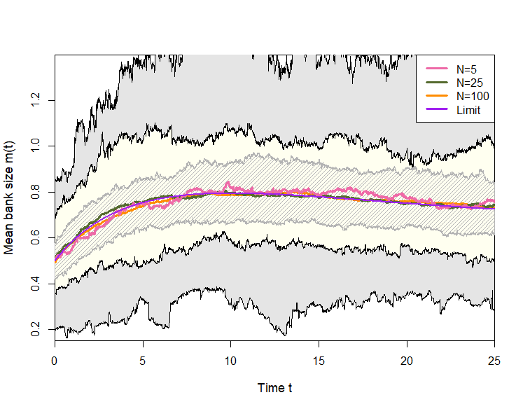
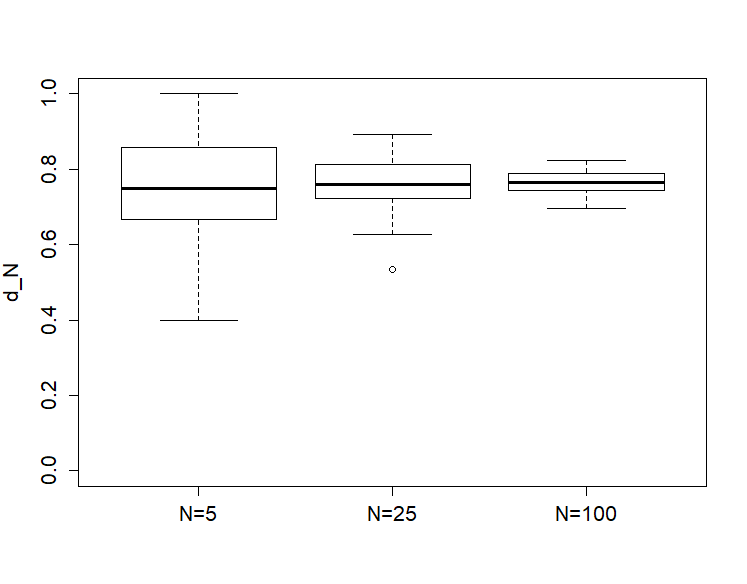
Figure 4. Left panel: distribution of $m_{N}(t)$ on $t\in[0,25]$ and $N=5,25,100$ based on $100$ simulated trajectories of $X^{(N)}$. The initial distribution is $\mu^{(N)}_{0}\sim\operatorname{Exp}(2)$, so $m_{N}(0)=0.5$. The deterministic limit $\mathbf{\tilde{m}}(\cdot)$ is also shown. Right panel: distribution of $d_{N}:=(\mu^{(N)}_{T},1_{[0,D]})$, proportion of banks with reserves less than $D=1$ at $T=25$.

Corollary 32.

We work under Assumptions 24, 25, 26, 27. Assume $X_{1}^{(N)}(0)$ is deterministic for every $N\geq 1$, and $X_{1}^{(N)}(0)\to x_{1}$ as $N\to\infty$. As $N\to\infty$, $X_{1}^{(N)}\Rightarrow X^{(\infty)}_{1}$ weakly in $\mathcal{D}[0,T]$, where $X^{(\infty)}_{1}$ is a solution to

(5.13) $$\mathrm{d}X^{(\infty)}_{1}(t)=\tilde{\psi}\bigl{(}t,X^{(\infty)}_{1}(t),\mathbf{\tilde{m}}(t)\bigr{)}X^{(\infty)}_{1}(t)\,\mathrm{d}t+\sigma X^{(\infty)}_{1}(t)\,\mathrm{d}W(t),$$

starting from $x_{1}$, killed with rate $\kappa_{\infty}(\mathbf{\tilde{m}}(t),X^{(\infty)}_{1}(t))$.

6. Proofs for Sections 2 and 3

We start with the following three technical lemmata and their proofs.

Lemma 33.

If $\nu_{n}\to\nu_{0}$ in $\mathcal{W}_{p}$ for some $p\geq 1$, then $(\nu_{n},f)\to(\nu_{0},f)$ for functions $f:\mathbb{R}_{+}\to\mathbb{R}$ with the following property:

$$C_{f}:=\sup_{x\geq 1}\left[x^{-q}|f(x)|\right]<\infty\quad\mbox{for some}\quad 0<q<p.$$

In particular, the functional of taking the mean $\nu\mapsto\overline{\nu}$ is continuous in $\mathcal{W}_{p}$.

Lemma 34.

For $0<q<p$ and any $C>0$, the set $\{\nu\in\mathcal{P}_{p}\,:\,(\nu,f_{p})\leq C\}$ is precompact in $\mathcal{P}_{q}$.

Lemma 35.

For every $\varepsilon\in(0,1)$, there exists a constant $C_{\varepsilon}$ such that for every function $f\in\mathcal{C}^{2}_{b}$, and for $x>0$, $z\in(0,1-\varepsilon)$, we have:

$$\left|f(x(1-z))-f(x)-zD_{1}f(x)\right|\leq C_{\varepsilon}z^{2}{|\kern-1.07639pt|\kern-1.07639pt|f|\kern-1.07639pt|\kern-1.07639pt|}.$$

6.1. Proof of Lemma 33

Let us take a sequence $(\xi_{n})$ of random variables: $\xi_{n}\sim\nu_{n}$ for every $n$. By the Skorohod representation theorem, we can assume $\xi_{n}\to\xi_{0}$ a.s., as $n\to\infty$. We also have $\mathbb{E}\lvert\xi_{n}\rvert^{p}\to\mathbb{E}\lvert\xi_{0}\rvert^{p}$, as $\nu_{n}\to\nu_{0}$ in the Wasserstein metric $\mathcal{W}_{p}$. Since $|f(x)|^{p/q}\leq C_{f}^{p/q}x^{p}$ for $f\in\mathcal{H}_{q}$, we get $\sup_{n\geq 1}\mathbb{E}\left[\lvert f(\xi_{n})\rvert^{p/q}\right]<\infty$. Thus for $p>q$ the family $(f(\xi_{n}))_{n\geq 1}$ is uniformly integrable, and hence, $(\nu_{n},f)=\mathbb{E}f(\xi_{n})\to\mathbb{E}f(\xi_{0})=(\nu_{0},f)$ as $n\to\infty$.

6.2. Proof of Lemma 34

Take a sequence $(\nu_{n})_{n\geq 1}$ of measures in $\{\nu\in\mathcal{P}_{p}:(\nu,f_{p})\leq C\}$, and generate random variables $\xi_{n}\sim\nu_{n}$. Since $\sup_{n\geq 1}\mathbb{E}\lvert\xi_{n}\rvert^{p}\leq C<\infty,$ the sequence $(\xi_{n})_{n\geq 1}$ is tight. Extract a weakly convergent subsequence; without loss of generality, we assume this sequence itself converges weakly to some random variable $\xi_{0}$. By the Skorohod representation theorem, we can assume $\xi_{n}\to\xi_{0}$ a.s. Moreover, the sequence $(\lvert\xi_{n}\rvert^{q})_{n\geq 1}$ is uniformly integrable for $q<p$, since $\mathbb{E}[(\lvert\xi_{n}\rvert^{q})^{p/q}]\leq C$. Therefore, $\mathbb{E}\lvert\xi_{n}\rvert^{q}\to\mathbb{E}\lvert\xi_{0}\rvert^{q}$, and hence, $\xi_{n}\to\xi_{0}$ in $\mathcal{W}_{q}$.

6.3. Proof of Lemma 35

Take a function $g(x):=f(e^{x})$. Then

$$g^{\prime}(x)=e^{x}f^{\prime}(e^{x})=(D_{1}f)(e^{x}),\quad g^{\prime\prime}(x)=e^{x}f^{\prime}(e^{x})+e^{2x}f^{\prime\prime}(e^{x})=(D_{1}f+D_{2}f)(e^{x}).$$

We can rewrite it for some $y\in[\ln x+\ln(1-z),\ln x]$:

$$f(x(1-z)) -f(x)-zD_{1}f(x)$$

$$=g(\ln x+\ln(1-z))-g(\ln x)-zg^{\prime}(\ln x)$$

$$=g(\ln x+\ln(1-z))-g(\ln x)+\ln(1-z)g^{\prime}(\ln x)-(\ln(1-z)+z)g^{\prime}(\ln x)$$

$$=\frac{1}{2}\ln^{2}(1-z)g^{\prime\prime}(y)-(\ln(1-z)+z)g^{\prime}(\ln x).$$

There exists a $C_{\varepsilon}$ such that for $z\in[0,1-\varepsilon]$,

$$\frac{1}{2}\ln^{2}(1-z)\leq C_{\varepsilon}z^{2},\quad\ln(1-z)+z\leq C_{\varepsilon}z^{2}.$$

It suffices to note that for all $y\in\mathbb{R}$, we have: $|g^{\prime\prime}(y)|\leq{|\kern-1.07639pt|\kern-1.07639pt|f|\kern-1.07639pt|\kern-1.07639pt|}$; and for all $x>0$, we have: $|g^{\prime}(\ln x)|\leq{|\kern-1.07639pt|\kern-1.07639pt|f|\kern-1.07639pt|\kern-1.07639pt|}$. This completes the proof.

6.4. Proof of Lemma 1

We need to establish (3.1), i.e., $P^{t}(\mathbf{x},A)>0\ \forall t>0$. Assume first that $A\subseteq(0,\infty)^{N}$ for $N=\mathfrak{n}(\mathbf{x})\geq 1$; that is, the target set $A$ lies on the same level as the initial point $\mathbf{x}$. Observe that the intensities of births and defaults of banks are locally bounded on $(0,\infty)^{N}$ as long as there are $N$ banks in the system; therefore, with positive probability there are $N$ banks at every time $s\in[0,t]$, and the process $X$ behaves as the solution to a certain stochastic differential equation on $(0,\infty)^{N}$ with a nonsingular covariance matrix. But such processes have the positivity property.

If $N=\mathfrak{n}(\mathbf{x})=0$, and $A=\{\varnothing\}$, then $P^{t}(\mathbf{x},A)=e^{-\lambda_{0}t}>0$: This is the probability that, starting with an empty system, no banks emerged during time $[0,t]$.

Assume now that $A\subseteq(0,\infty)^{M}$ for $M\neq N=\mathfrak{n}(\mathbf{x})\geq 1$. Then with positive probability we have: $\mathfrak{n}(X(s))=M$ for some $s\in[0,t)$, since the rates of birth and default are everywhere positive. Let $\tau^{\prime}$ be the first moment of hitting level $M$:

$$\tau^{\prime}:=\inf\{s\geq 0\mid\mathfrak{n}(X(s))=M\}.$$

Observe that the integral of a positive function over a set of positive measure is positive. Applying this and conditioning on $\tau^{\prime}$ and $X(\tau^{\prime})$, by the Markov property of $X$ we get:

$$\mathbb{P}(X(t)\in A)=\int_{0}^{t}\mathbb{P}(\tau^{\prime}\in\mathrm{d}s,\,X(\tau^{\prime})\in\mathrm{d}\mathbf{y})\,\mathbb{P}\left(X(t-s)\in A\mid X(0)=\mathbf{y}\right)>0.$$

This completes the proof of (3.1) for subsets $A$ which are on one level of $\mathcal{X}$. Any general set $A\subseteq\mathcal{X}$ can be split into its subsets, at least one of which has positive Lebesgue measure.

6.5. Proof of Theorem 3

The statement of Theorem 3 then follows from Lemmata 1, 2, and the classic results of [MT93a, MT93b], together with [Sar17, Proposition 2.2, Lemma 2.3]. In fact, since the last two terms in (3.3) are non-positive, the condition in Theorem 3 is effectively about the term due to births $\lambda_{\mathfrak{n}(\mathbf{x})}(\mathfrak{s}(\mathbf{x}))\left[\overline{\mathcal{B}}(\mathfrak{n}(\mathbf{x}),\mathfrak{s}(\mathbf{x}))+1\right],$ growing at most linearly in $\mathfrak{n}(x)$ and $\mathfrak{s}(x)$.

6.6. Proof of Theorem 7

Without loss of generality, assume $c_{1}=c_{2}=c$ by taking the smaller one among $c_{1}$ and $c_{2}$. Compare (3.3) with (3.6) and observe that for every $\varepsilon\in(0,1)$

$$\mathfrak{L}V_{0}(\mathbf{x})=\varphi(\mathbf{x})\leq-cV_{0}(\mathbf{x})+c_{3}\leq-(1-\varepsilon)cV_{0}(\mathbf{x})+c_{3}\cdot 1_{\mathcal{K}}(\mathbf{x}),\ \mathbf{x}\in\mathcal{X},$$

where $\mathcal{K}:=\{\mathbf{x}\in\mathcal{X}:V_{0}(\mathbf{x})\leq c_{3}/(\varepsilon c)\}$ is a compact subset of $\mathcal{X}$. The bound (3.7) follows from Lemmata 1, 2, and from the theory of Lyapunov functions, e.g. [MT93a, MT93b, Sar17]

6.7. Proof of Theorem 9

Take two copies $X^{(1)}=(X^{(1)}(t),\,t\geq 0)$ and $X^{(2)}=(X^{(2)}(t),\,t\geq 0)$ of this process, starting from $X^{(1)}(0)=\mathbf{x}_{1}$ and $X^{(2)}(0)=\mathbf{x}_{2}$. The idea is to couple them when the dimension-counting processes $N^{(1)}(\cdot)=\mathfrak{n}(X^{(1)}(\cdot))$ and $N^{(2)}(\cdot)=\mathfrak{n}(X^{(2)}(\cdot))$ meet at $0$. Then the original processes $X^{(1)}$ and $X^{(2)}$ meet at $\varnothing$. Define this coupling time $\tau$:

(6.1) $$\tau:=\inf\{t\geq 0\mid N^{(1)}(t)=N^{(2)}(t)=0\}.$$

By classic Lindvall’s inequality, the total variation distance from (2.7) between $P^{t}(\mathbf{x}_{1},\cdot)$ and $P^{t}(\mathbf{x}_{2},\cdot)$ is less than or equal to $2\,\mathbb{P}(\tau\geq t)$. Next, compare these dimension-counting processes $N^{(i)}$ with birth-death processes: $N^{(i)}(t)=\mathfrak{n}(X^{(i)}(t))\leq\hat{N}^{(i)}(t)$, $i=1,2$, $\,t\geq 0$, where $\hat{N}^{(i)}=(\hat{N}^{(i)}(t),\,t\geq 0)$ is a birth-death process with birth intensity $\lambda^{*}_{n}$ and death intensity $n\kappa^{*}_{n}$ at site $n\in\mathbb{Z}_{+}$, starting from $\hat{N}^{(i)}(0):=N^{(i)}(0)$, $i=1,2$. Similarly to [LMT96, Sar16], we find that the moment $\tau$ satisfies the following estimate:

(6.2) $$\mathbb{E}[e^{\alpha\tau}]\leq\hat{V}(\hat{N}^{(1)}(0)\vee\hat{N}^{(2)}(0))=\tilde{V}(\mathbf{x}_{1})\vee\tilde{V}(\mathbf{x}_{2}).$$

The coupling time (6.1) for the processes $\hat{N}^{(1)}$ and $\hat{N}^{(2)}$ is also a coupling time for the processes $X^{(1)}$ and $X^{(2)}$. The rest of the proof is similar to [LMT96, Theorem 2.2], [Sar16, Section 5].

7. Proof of Theorem 21

7.1. Overview of the proof

Recall the definition of $\mathcal{E}_{f}$ from (2.2). Itô’s formula applied to $\mathcal{E}_{f}(X^{(N)}(t))=(\mu^{(N)}_{t},f)$ for some function $f\in\mathcal{C}_{b}^{2}$ reads as:

(7.1) $$\mathcal{E}_{f}\left(X^{(N)}(t)\right)=\mathcal{E}_{f}\left(X^{(N)}(0)\right)+\int_{0}^{t}\mathcal{L}\mathcal{E}_{f}\bigl{(}X^{(N)}(s)\bigr{)}\,\mathrm{d}s+\mathcal{M}_{N}^{f}(t),$$

where $(\mathcal{M}_{N}^{f}(t),\,t\geq 0)$ is a real-valued rcll local martingale. Between jumps (while the number of banks $\mathfrak{n}(X^{(N)}(t))=\mathcal{N}_{N}(t)$ stays constant), the local martingale $\mathcal{M}_{N}^{f}$ is given by

$$\mathrm{d}\mathcal{M}_{N}^{f}(t):=\frac{\sigma}{\mathcal{N}_{N}(t)}\sum\limits_{i=1}^{\mathcal{N}_{N}(t)}(D_{1}f)\bigl{(}X_{i}^{(N)}(t)\bigr{)}\,\mathrm{d}W_{i}(t).$$

First, let us state the main convergence lemma, which makes the analytical crux of the proof.

Lemma 36.

Take a function $f\in\mathcal{C}^{2}_{b}$. Recalling (2.1), take a sequence $(\mathbf{x}^{(k)})_{k\geq 1}$ in $\mathfrak{X}$ with

(7.2) $$\mathfrak{n}\left(\mathbf{x}^{(k)}\right)=k\quad\mbox{and}\quad\mu_{\mathbf{x}^{(k)}}\to\nu\quad\mbox{in}\ \mathcal{W}_{p}\quad\text{as}\quad k\to\infty.$$

Then we have the following convergence of means and generators, as $N\to\infty$:

(7.3) $$\overline{\mathbf{x}}^{(k)}\to\overline{\nu};\quad\mbox{and}\quad\mathfrak{L}\mathcal{E}_{f}\left(\mathbf{x}^{(k)}\right)\to\mathcal{A}(\nu,f)\quad\text{from}\quad\eqref{eq:main-operator}.$$

The following technical estimate is used repeatedly in the subsequent proofs.

Lemma 37.

For a constant $C$ depending on the parameters, we have

$$\left|\mathfrak{L}\mathcal{E}_{f}(\mathbf{x})\right|\leq C\left[1+\overline{\mathbf{x}}\right]\cdot{|\kern-1.07639pt|\kern-1.07639pt|f|\kern-1.07639pt|\kern-1.07639pt|},\quad f\in\mathcal{C}^{2}_{b},\quad\mathbf{x}\in\mathcal{X}\setminus\{\varnothing\}.$$

We next show that the term $\mathcal{M}_{N}^{f}$ tends to zero. The rough idea is as follows: Since jump sizes tend to zero, the process converges to a continuous limit. Since the quadratic variation converges to zero, the limit is a continuous martingale with zero quadratic variation, which implies that the limit itself is identically zero. To formalize this argument and apply it to our more complicated situation, we state and prove the following series of lemmata.

Lemma 38.

For every $T>0$, $r>1$, and $f\in\mathcal{C}^{2}_{b}$,

$$\mathbb{E}\Big{[}\sup\limits_{0\leq s\leq T}\bigl{[}\mathcal{M}_{N}^{f}(s)\bigr{]}^{r}\Big{]}\to 0,\quad\mbox{as}\quad N\to\infty.$$

Lemma 39.

For every $T>0$, there exists a constant $C_{T}>0$ such that

$$\mathbb{E}\Big{[}\sup\limits_{t\in[0,T]}\bigl{(}\mu^{(N)}_{t},f_{p}\bigr{)}\Big{]}\leq C_{T}\quad\mbox{for all}\quad N\geq 1.$$

Lemma 40.

The sequence $(\mu^{(N)}_{t},\,0\leq t\leq T)_{N\geq 1}$ is tight in $\mathcal{D}([0,T],\mathcal{P}_{q})$ for every $q<p$.

Assume we already proved Lemmata 36, 38, 39, 40. Let us complete the proof of Theorem 21. In light of Lemma 40, it suffices to show the following statement: For $q\in[1,p)$, every weak limit point $\bigl{(}\mu^{(\infty)}_{t},\,t\in[0,T]\bigr{)}$ of $\bigl{(}\mu^{(N)}_{t},\,0\leq t\leq T\bigr{)}_{N\geq 1}$ in $\mathcal{D}([0,T],\mathcal{P}_{q})$ is governed by the McKean-Vlasov equation (4.17). Indeed, for any function $f\in\mathcal{C}^{2}_{b}$, we can rewrite (7.1) as follows:

(7.4) $$\bigl{(}\mu^{(N)}_{t},f\bigr{)}=\bigl{(}\mu^{(N)}_{0},f\bigr{)}+\int_{0}^{t}\mathcal{L}\mathcal{E}_{f}\left(X^{(N)}(s)\right)\,\mathrm{d}s+\mathcal{M}^{f}_{N}(t).$$

Lettting $N\to\infty$ in (7.4) with Lemmata 36,  38 and 39, we have that the last term vanishes while the key middle term converges to $\mathcal{A}(\mu^{(\infty)}_{s},f)$. Overall we thus obtain that the limit obeys

$$\bigl{(}\mu^{(\infty)}_{t},f\bigr{)}=\bigl{(}\mu^{(\infty)}_{0},f\bigr{)}+\int_{0}^{t}\mathcal{A}(\mu^{(\infty)}_{s},f)\,\mathrm{d}s.$$

Since this holds true for all $f\in\mathcal{C}^{2}_{b}$, then, as explained in subsection 4.1, this is the equivalent definition of the McKean-Vlasov jump-diffusion. This completes the proof of Theorem 21.

7.2. Proof of Lemma 36

Convergence of means follows from Lemma 33. Now, let us show the second statement in (7.3). Apply the generator $\mathfrak{L}$ from (2.10) to $\mathcal{E}_{f}$ from (2.2), for $f\in\mathcal{C}^{2}$, with the argument $\mathbf{x}=\bigl{(}x_{1},\ldots,x_{\mathfrak{n}(\mathbf{x})}\bigr{)}\neq\varnothing$. At first, we just do calculations of the generator, and only afterwards we plug in $\mathbf{x}^{(k)}$ instead of $\mathbf{x}$. Corresponding to the three lines in the right-hand side of (2.10) we shall use the shorthand $\mathfrak{L}\,\mathcal{E}_{f}=I_{1}+I_{2}+I_{3}$. The first term $I_{1}$ involving the diffusion operator is calculated as follows:

$$\frac{\partial\mathcal{E}_{f}}{\partial x_{i}}(\mathbf{x})=\frac{1}{\mathfrak{n}(\mathbf{x})}f^{\prime}(x_{i}),\quad\frac{\partial^{2}\mathcal{E}_{f}}{\partial x_{i}^{2}}(\mathbf{x})=\frac{1}{\mathfrak{n}(\mathbf{x})}f^{\prime\prime}(x_{i}),\quad i=1,\ldots,\mathfrak{n}(\mathbf{x}),$$

which leads to

(7.5) $$I_{1}=\frac{1}{\mathfrak{n}(\mathbf{x})}\sum\limits_{i=1}^{\mathfrak{n}(\mathbf{x})}\Bigl{[}rx_{i}f^{\prime}(x_{i})+\frac{\sigma^{2}}{2}x_{i}^{2}f^{\prime\prime}(x_{i})\Bigr{]}=\frac{1}{\mathfrak{n}(\mathbf{x})}\sum\limits_{i=1}^{\mathfrak{n}(\mathbf{x})}\mathcal{G}f(x_{i})=(\mu_{\mathbf{x}},\mathcal{G}f).$$

Next, the second term with the birth rates is equal to

(7.6) $$\begin{split}I_{2}&=\lambda_{\mathfrak{n}(x)}(\mathfrak{s}(\mathbf{x}))\int_{0}^{\infty}\Bigl{[}\frac{1}{\mathfrak{n}(\mathbf{x})+1}\Bigl{(}\sum\limits_{i=1}^{\mathfrak{n}(\mathbf{x})}f(x_{i})+f(y)\Bigr{)}-\frac{1}{\mathfrak{n}(\mathbf{x})}\sum\limits_{i=1}^{\mathfrak{n}(\mathbf{x})}f(x_{i})\Bigr{]}\,\mathcal{B}_{\mathfrak{n}(\mathbf{x}),\mathfrak{s}(\mathbf{x})}(\mathrm{d}y)\\ &=-\frac{1}{\mathfrak{n}(\mathbf{x})(1+\mathfrak{n}(\mathbf{x}))}\lambda_{\mathfrak{n}(\mathbf{x})}(\mathfrak{s}(\mathbf{x}))\sum\limits_{i=1}^{\mathfrak{n}(\mathbf{x})}f(x_{i})+\frac{\lambda_{\mathfrak{n}(\mathbf{x})}(\mathfrak{s}(\mathbf{x}))}{\mathfrak{n}(\mathbf{x})+1}\int_{0}^{\infty}f(y)\,\mathcal{B}_{\mathfrak{n}(\mathbf{x}),\mathfrak{s}(\mathbf{x})}(\mathrm{d}y)\\ &=-\frac{\lambda_{\mathfrak{n}(\mathbf{x})}(\mathfrak{s}(\mathbf{x}))}{\mathfrak{n}(\mathbf{x})+1}\left(\mu_{\mathbf{x}},f\right)+\frac{\lambda_{\mathfrak{n}(\mathbf{x})}(\mathfrak{s}(\mathbf{x}))}{\mathfrak{n}(\mathbf{x})+1}\int_{0}^{\infty}f(y)\,\mathcal{B}_{\mathfrak{n}(\mathbf{x}),\mathfrak{s}(\mathbf{x})}(\mathrm{d}y).\end{split}$$

Finally, the third term is

$$I_{3}=\sum\limits_{i=1}^{\mathfrak{n}(\mathbf{x})} \kappa_{\mathfrak{n}(\mathbf{x})}(\mathfrak{s}(\mathbf{x}),x_{i})\frac{1}{\mathfrak{n}(\mathbf{x})-1}\sum\limits_{j\neq i}^{\mathfrak{n}(\mathbf{x})}\int_{0}^{1}f(x_{j}(1-z_{j}))\,\mathcal{D}_{\mathfrak{n}(\mathbf{x}),\mathfrak{s}(\mathbf{x}),x_{i}}(\mathrm{d}z_{j})$$

$$-\frac{1}{\mathfrak{n}(\mathbf{x})}\sum\limits_{i=1}^{\mathfrak{n}(\mathbf{x})}\kappa_{\mathfrak{n}(\mathbf{x})}(\mathfrak{s}(\mathbf{x}),x_{i})\sum\limits_{j=1}^{\mathfrak{n}(\mathbf{x})}\int_{0}^{1}f(x_{j})\,\mathcal{D}_{\mathfrak{n}(\mathbf{x}),\mathfrak{s}(\mathbf{x}),x_{i}}(\mathrm{d}z_{j}),$$

which we re-arrange as

(7.7) $$\begin{split}I_{3}&=\frac{1}{\mathfrak{n}(\mathbf{x})}\sum\limits_{i=1}^{\mathfrak{n}(\mathbf{x})}\kappa_{\mathfrak{n}(\mathbf{x})}(\mathfrak{s}(\mathbf{x}),x_{i})\sum\limits_{j=1}^{\mathfrak{n}(\mathbf{x})}\int_{0}^{1}\left[f(x_{j}(1-z_{j}))-f(x_{j})\right]\,\mathcal{D}_{\mathfrak{n}(\mathbf{x}),\mathfrak{s}(\mathbf{x}),x_{i}}(\mathrm{d}z_{j})\\ &+\frac{1}{\mathfrak{n}(\mathbf{x})(\mathfrak{n}(\mathbf{x})-1)}\sum\limits_{i=1}^{\mathfrak{n}(\mathbf{x})}\kappa_{\mathfrak{n}(\mathbf{x})}(\mathfrak{s}(\mathbf{x}),x_{i})\sum\limits_{j=1}^{\mathfrak{n}(\mathbf{x})}\int_{0}^{1}f(x_{j}(1-z_{j}))\,\mathcal{D}_{\mathfrak{n}(\mathbf{x}),\mathfrak{s}(\mathbf{x}),x_{i}}(\mathrm{d}z_{j})\\ &-\frac{1}{\mathfrak{n}(\mathbf{x})-1}\sum\limits_{i=1}^{\mathfrak{n}(\mathbf{x})}\kappa_{\mathfrak{n}(\mathbf{x})}(\mathfrak{s}(\mathbf{x}),x_{i})\int_{0}^{1}f(x_{i}(1-z_{i}))\,\mathcal{D}_{\mathfrak{n}(\mathbf{x}),\mathfrak{s}(\mathbf{x}),x_{i}}(\mathrm{d}z_{i})=:I_{3,1}+I_{3,2}+I_{3,3}.\end{split}$$

Now, substitute the following sequence in the formulae above:

(7.8) $$\mathbf{x}:=\mathbf{x}^{(k)},\quad\mathfrak{n}\bigl{(}\mathbf{x}^{(k)}\bigr{)}=k,\quad s_{k}:=\mathfrak{s}\left(\mathbf{x}^{(k)}\right).$$

The first term of $\mathfrak{L}\mathcal{E}_{f}\left(\mathbf{x}^{(k)}\right)$, given in (7.5), converges as $k\to\infty$ as follows:

(7.9) $$I_{1}=(\mu_{\mathbf{x}^{(k)}},\mathcal{G}f)\to(\nu,\mathcal{G}_{\overline{\nu}}f).$$

This follows from the observation that $\mathcal{G}f\in\mathcal{H}_{q}$, and Lemma 33. Next, we get convergence of the second term $I_{2}$ given in (7.6):

(7.10) $$I_{2}\to\lambda_{\infty}\left(\overline{\nu}\right)\left(\mathcal{B}_{\infty,\overline{\nu}},f\right)-\lambda_{\infty}\left(\overline{\nu}\right)\left(\nu,f\right)$$

from Assumptions 15 and 16, together with the observation that $f\in\mathcal{C}^{2}_{b}$, and another application of Lemma 33. Finally, let us show convergence of $I_{3}$ from (7.7), i.e.,

(7.11) $$I_{3}\to-\left(\nu,\kappa_{\infty}\left(\overline{\nu},\cdot\right)f\right)+(\nu,f)\left(\nu,\kappa_{\infty}\left(\overline{\nu},\cdot\right)\right),\quad\text{ as }\quad k\to\infty.$$

The first term $I_{3,1}$ in (7.7) can be expressed, using Lemma 35:

(7.12) $$I_{3,1}=-\frac{1}{k}\sum\limits_{i=1}^{k}\kappa_{k}(s_{k},x^{(k)}_{i})\cdot\sum\limits_{j=1}^{k}D_{1}f(x^{(k)}_{j})\int_{0}^{1}z\,\mathcal{D}_{k,s_{k},x^{(k)}_{i}}(\mathrm{d}z)+\delta_{k}=:J_{k}+\delta_{k},$$

where the residual $\delta_{k}$ for $k\geq n_{0}$ can be estimated as

$$|\delta_{k}|\leq C_{\varepsilon_{0}}{|\kern-1.07639pt|\kern-1.07639pt|f|\kern-1.07639pt|\kern-1.07639pt|}\cdot\frac{1}{k}\sum\limits_{i=1}^{k}\kappa_{k}(s_{k},x^{(k)}_{i})\cdot k\cdot\int^{1}_{0}z^{2}\mathcal{D}_{k,s_{k},x_{i}^{(k)}}({\mathrm{d}}z).$$

By Remark 4.9 and Assumption 19,

(7.13) $$|\delta_{k}|\leq k^{-1}C_{\varepsilon_{0}}C_{\kappa}C_{\mathcal{D},2}\cdot{|\kern-1.07639pt|\kern-1.07639pt|f|\kern-1.07639pt|\kern-1.07639pt|}.$$

Finally, the main term $J_{k}$ in (7.12) of $I_{3,1}$ can be written as

$$J_{k} =-\frac{1}{k}\sum\limits_{i=1}^{k}\kappa_{k}(s_{k},x^{(k)}_{i})\cdot\frac{1}{k}\sum\limits_{j=1}^{k}kD_{1}f(x^{(k)}_{j})\overline{\mathcal{D}}(k,s_{k},x^{(k)}_{i})$$

(7.14) $$=-\left(\mu_{\mathbf{x}^{(k)}},k\overline{\mathcal{D}}(k,s_{k},\cdot)\kappa_{k}(s_{k},\cdot)\right)\left(\mu_{\mathbf{x}^{(k)}},D_{1}f\right).$$

As $k\to\infty$, the expression (7.14) tends to

(7.15) $$\lim_{k\to\infty}J_{k}=-\left(\nu,\kappa_{\infty}(\overline{\nu},\cdot)\overline{\mathcal{D}}_{\infty}(\overline{\nu},\cdot)\right)\left(\nu,D_{1}f\right).$$

From (7.12), (7.13), and (7.15), we get

(7.16) $$I_{3,1}\to-\left(\nu,\kappa_{\infty}(\overline{\nu},\cdot)\overline{\mathcal{D}}_{\infty}(\overline{\nu},\cdot)\right)\left(\nu,D_{1}f\right),$$

which becomes the mean-field drift term in (4.11). Similarly, we can show that the second and third terms $I_{3,2},I_{3,3}$ in (7.7) converge respectively to:

(7.17) $$\lim_{k\to\infty}I_{3,2}=+(\nu,f)\left(\nu,\kappa_{\infty}\left(\overline{\nu},\cdot\right)\right)\quad\mbox{and}\quad\lim\limits_{k\to\infty}I_{3,3}=-\left(\nu,\kappa_{\infty}\left(\overline{\nu},\cdot\right)f\right)\quad$$

Let us show this for $I_{3,2}$; the proof for $I_{3,3}$ is similar. It follows from Assumption 17 that the default contagion measures $\mathcal{D}_{\cdot,\cdot,\cdot}$ converge to $\delta_{0}$ (delta mass measure at zero) uniformly in $\mathcal{W}_{p}$. Because $f\in\mathcal{C}^{2}_{b}$, we have the following convergence as $k\to\infty$, uniformly over $j$:

$$\int_{0}^{1}f(x_{j}(1-z_{j}))\,\mathcal{D}_{k,s_{k},x^{(k)}_{i}}(\mathrm{d}z_{j})\to f(x_{j}),$$

which together with the assumption (7.2) yields

(7.18) $$\frac{1}{k}\sum\limits_{j=1}^{k}\int_{0}^{1}f(x_{j}(1-z_{j}))\,\mathcal{D}_{k,s_{k},x^{(k)}_{i}}(\mathrm{d}z_{j})\to(\nu,f),$$

as $k\to\infty$. Finally, by uniform boundedness of $\kappa_{\cdot}(\cdot,\cdot)$ together with (7.2), we get:

(7.19) $$\frac{1}{k}\sum\limits_{i=1}^{k}\kappa_{k}\bigl{(}s_{k},x_{i}^{(k)}\bigr{)}\to\bigl{(}\nu,\kappa_{\infty}\bigl{(}\overline{\nu},\cdot\bigr{)}\bigr{)}.$$

Combined, (7.16) and (7.17) complete the proof of (7.11), and of Lemma 36.

7.3. Proof of Lemma 37

From Assumptions 15, 16, 17, 19, we estimate separately each term for $f$ in $\mathfrak{L}\,\mathcal{E}_{f}(x)=I_{1}+I_{2}+I_{3}$, given in (7.5)-(7.7). The first term from (7.5) is estimated as:

$$|I_{1}|\leq r\left\lVert D_{1}f\right\rVert+\frac{\sigma^{2}}{2}\left\lVert D_{2}f\right\rVert.$$

For the second term in (7.6), from Assumption 16, we get:

$$|I_{2}|\leq 2C_{\lambda}\left\lVert f\right\rVert\left(1+\overline{\mathbf{x}}\right).$$

Finally, consider the third term in (7.7). Via Assumptions 17 and 19, similarly to the proof of Lemma 36, this term is estimated as

$$|I_{3}|\leq 2C_{\kappa}\left\lVert f\right\rVert+C_{\kappa}C_{\mathcal{D},1}\left\lVert D_{1}f\right\rVert+C_{\kappa}C_{\mathcal{D},2}\left\lVert D_{2}f\right\rVert+C_{\kappa}C_{\varepsilon_{0}}C_{\mathcal{D},2}\cdot{|\kern-1.07639pt|\kern-1.07639pt|f|\kern-1.07639pt|\kern-1.07639pt|},$$

where $C_{\mathcal{D},p}$ was defined in (4.9). Combining these estimates, we complete the proof of Lemma 37.

7.4. Estimation of the number of banks from above and below

These results will be needed for the proof of Lemma 39 and Lemma 40. Define the minimal and maximal number of banks in the system $X^{(N)}$ on time horizon $[0,T]$:

$$\mathfrak{M}^{-}_{N}(T):=\min\limits_{0\leq t\leq T}\mathcal{N}_{N}(t),\quad\mathfrak{M}^{+}_{N}(T):=\max\limits_{0\leq t\leq T}\mathcal{N}_{N}(t).$$

We start by estimating $\mathfrak{M}^{-}_{N}(T)$ from below. First, we claim that $\mathfrak{M}^{-}_{N}(T)$ stochastically dominates a Binomial random variable $\xi_{N}$ with parameters $\xi_{N}\sim\mathrm{Bin}(N,e^{-C_{\kappa}T})$ with mean $\bar{\xi}:=Ne^{-C_{\kappa}T}$. Indeed, $\mathcal{N}_{N}(0)=N$, and the default intensities are uniformly bounded from above by the constant $C_{\kappa}$. Then assume there is no birth of new banks, and all default intensities are exactly $C_{\kappa}$ on $[0,T]$ as an extreme case. This makes the number of banks at $T$ fewer than for our original system $X^{(N)}$ and distributed as the binomial random variable $\xi_{N}$. The latter tends to infinity in law: $\mathfrak{M}^{-}_{N}(T)\to\infty$ as $N\to\infty$ from Chernov’s inequality

(7.20) $$\mathbb{P}\big{(}\xi_{N}\leq\bar{\xi}/2\big{)}\leq\exp\left(-\bar{\xi}/8\right)$$

and from it, we get the following estimate: there exists a constant $C_{\mathfrak{M}}$ such that

(7.21) $$\mathbb{E}\left[(\mathfrak{M}^{-}_{N}(T)\vee 1)^{-r}\right]\leq\mathbb{E}\left[(\xi_{N}\vee 1)^{-r}\right]\leq\left(\bar{\xi}/2\right)^{-r}+\exp\left(-\bar{\xi}/8\right)\leq C_{\mathfrak{M}}N^{-r},\quad r>0.$$

Now, let us estimate the maximal number of banks from above. Consider a pure birth process $\beta_{N}=(\beta_{N}(t),\,t\geq 0)$ on $\{1,2,\ldots\}$ starting from $\beta_{N}(0)=N$, such that the intensity of births from level $n$ to $n+1$ is equal to $C_{\lambda}n$. Recall the estimate $\lambda_{N}(s)\leq C_{\lambda}N$ in Assumption 16. We have the following observation: If there are no defaults, then $\mathcal{N}_{N}(t)$ is dominated by the above birth process $\beta_{N}$: $\mathcal{N}_{N}(t)\leq\beta_{N}(T)$, where $\beta_{N}(0)=N$. At the same time,

$$d\mathbb{E}[\beta_{N}(t)]/dt=C_{\lambda}\mathbb{E}[\beta_{N}(t)],\quad\mbox{which implies}\quad\mathbb{E}[\beta_{N}(T)]=e^{C_{\lambda}T}N.$$

Therefore, for every $N\geq 1$,

(7.22) $$\mathbb{E}\left[\mathfrak{M}^{+}_{N}(T)\right]\leq e^{C_{\lambda}T}N.$$

What is more, we can estimate the second moment: The generator of $N^{-1}\beta_{N}$ is

$$\mathcal{L}_{N}f(x)=Nx\left(f(x+N^{-1})-f(x)\right).$$

Applying this to function $f:=f_{2}$, we get:

$$\mathcal{L}_{N}f_{2}(x)=2x^{2}+xN^{-1}.$$

If $m_{N}(t):=N^{-2}\mathbb{E}\beta_{N}^{2}(t)$, we can write Kolmogorov equations:

$$m^{\prime}_{N}(t)=\mathbb{E}[\mathcal{L}_{N}f_{2}(N^{-1}\beta_{N}(t))]=2m_{N}(t)+N^{-1}e^{C_{\lambda}T},\quad m_{N}(0)=1.$$

Solving this, it is easy to see that $\sup_{N}m_{N}(T)<\infty$. We can rewrite this as

(7.23) $$\mathbb{E}[\beta_{N}^{2}(T)]\leq C_{\beta}N^{2}.$$

7.5. Proof of Lemma 38

Consider the size of each jump of the process $\bigl{(}\mu^{(N)},f\bigr{)}$. At the emergence of a new bank with reserves $y$ at time $t$, the empirical measure process jumps

(7.24) $$\mbox{from}\quad\mu^{(N)}_{t-}=\frac{1}{\mathcal{N}_{N}(t-)}\sum\limits_{i=1}^{\mathcal{N}_{N}(t-)}\delta_{X^{(N)}_{i}(t-)}\quad\mbox{to}\quad\mu^{(N)}_{t}=\frac{1}{\mathcal{N}_{N}(t-)+1}\Biggl{[}\sum\limits_{i=1}^{\mathcal{N}_{N}(t-)}\delta_{X^{(N)}_{i}(t-)}+\delta_{y}\Biggr{]}.$$

Therefore, the displacement of $(\mu^{(N)},f)$ is equal to

$$\frac{1}{\mathcal{N}_{N}(t-)+1}\Biggl{[}\sum\limits_{i=1}^{\mathcal{N}_{N}(t-)}f\bigl{(}X_{i}^{(N)}(t-)\bigr{)}+f(y)\Biggr{]}-\frac{1}{\mathcal{N}_{N}(t-)}\sum\limits_{i=1}^{\mathcal{N}_{N}(t-)}f\bigl{(}X_{i}^{(N)}(t-)\bigr{)}.$$

This random variable is dominated a.s. by $2\left\lVert f\right\rVert/\mathcal{N}_{N}(t-)$. Similarly, at the default of the $i$th bank (assume without loss of generality that $i=1$), the displacement in $(\mu^{(N)},f)$ is

(7.25) $$\begin{split}\frac{1}{\mathcal{N}_{N}(t-)-1}&\sum\limits_{j=2}^{\mathcal{N}_{N}(t-)}f((1-z_{j})X^{(N)}_{j}(t-))-\frac{1}{\mathcal{N}_{N}(t-)}\sum\limits_{i=1}^{\mathcal{N}_{N}(t-)}f(X^{(N)}_{i}(t-)),\\ z_{j}&\sim\mathcal{D}_{\mathcal{N}_{N}(t-),\mathcal{S}_{N}(t-),X_{1}^{(N)}(t-)}.\end{split}$$

The expression in (7.25) is dominated by $2(\left\lVert D_{1}f\right\rVert+\left\lVert f\right\rVert)/\mathcal{N}_{N}(t-)$. To conclude, in both cases, recalling the definition of ${|\kern-1.07639pt|\kern-1.07639pt|\cdot|\kern-1.07639pt|\kern-1.07639pt|}$ in (2.6), the displacement of $(\mu^{(N)},f)$ is dominated by

(7.26) $$\frac{2}{\mathcal{N}_{N}(t-)}{|\kern-1.07639pt|\kern-1.07639pt|f|\kern-1.07639pt|\kern-1.07639pt|}.$$

Next, the quadratic variation $\langle\mathcal{M}_{N}^{f}\rangle$ satisfies

(7.27) $$\mathrm{d}\,\langle\mathcal{M}_{N}^{f}\rangle_{t}=\frac{\sigma^{2}}{\mathcal{N}_{N}(t)}\bigl{(}\mu^{(N)}_{t},(D_{1}f)^{2}\bigr{)}\,\mathrm{d}t.$$

From (7.27), it follows that

(7.28) $$\langle\mathcal{M}^{f}_{N}\rangle_{T}\leq\frac{\sigma^{2}}{\mathfrak{M}^{-}_{N}(T)}\int_{0}^{T}\left(\mu^{(N)}_{s},(D_{1}f)^{2}\right)\,\mathrm{d}s\leq\frac{\sigma^{2}T\cdot\left\lVert D_{1}f\right\rVert^{2}}{\mathfrak{M}_{N}^{-}(T)}.$$

On the time intervals when there are no banks at all, with $\mathcal{N}_{N}(t)=0$, the martingale $\mathcal{M}_{N}^{f}$ stays in fact constant, therefore we can neglect these intervals in our calculations. Apply (7.21) with $r/2$ instead of $r$ to get:

(7.29) $$\mathbb{E}\left[\langle\mathcal{M}^{f}_{N}\rangle_{T}\right]\to 0.$$

Next, from Lemma 37 we get that $(\mathcal{M}^{f}_{N})_{N\geq 1}$ is uniformly a.s. bounded on $[0,T]$ (by a constant $CT\cdot{|\kern-1.07639pt|\kern-1.07639pt|f|\kern-1.07639pt|\kern-1.07639pt|}+2\left\lVert f\right\rVert$). Extract a subsequence $(\mathcal{M}^{f}_{N_{j}}(T))_{j\geq 1}$ which converges a.s. and (by Lebesgue dominated convergence theorem) in $L^{2}$ to a random variable $\xi$. Let $\mathcal{M}_{\infty}^{f}(t):=\mathbb{E}(\xi\mid\mathfrak{F}_{t})$. Then by the standard martingale inequality

$$\mathbb{E}\sup\limits_{0\leq t\leq T}\bigl{(}\mathcal{M}_{\infty}^{f}(t)-\mathcal{M}_{N_{j}}^{f}\bigr{)}^{2}\leq 4\mathbb{E}\bigl{(}\xi-\mathcal{M}_{N_{j}}^{f}\bigr{)}^{2}\to 0.$$

Therefore, we can extract a subsequence such that

$$\mathcal{M}^{f}_{N_{j}^{\prime}}\to\mathcal{M}_{\infty}^{f}\quad\mbox{a.s.~{}uniformly on}\quad[0,T].$$

From (7.26), combined with estimates from below in subsection 7.4, we conclude that the process $\mathcal{M}_{\infty}^{f}$ is a.s. continuous. Moreover, it has zero quadratic variation by (7.29). Any continuous martingale with zero quadratic variation is constant. Therefore, $\mathcal{M}_{\infty}^{f}(t)=\mathcal{M}_{\infty}^{f}(0)=0$. Finally, every subsequence $(\mathcal{M}_{N}^{f})_{N\geq 1}$ contains its own subsequence which converges to $0$ uniformly in $L^{2}$. The result of Lemma 38 immediately follows from here.

7.6. Proof of Lemma 39

Recall that

$$\bigl{(}\mu^{(N)}_{t},f_{p}\bigr{)}=\frac{1}{\mathcal{N}_{N}(t)}\sum\limits_{i=1}^{\mathcal{N}_{N}(t)}\left[X_{i}^{(N)}(t)\right]^{p}\qquad\text{for }\quad\mathcal{N}_{N}(t)\geq 1.$$

If $\mathcal{N}_{N}(t)=0$, then $\bigl{(}\mu^{(N)}_{t},f_{p}\bigr{)}=0$. Therefore,

(7.30) $$\sup\limits_{0\leq t\leq T}\bigl{(}\mu^{(N)}_{t},f_{p}\bigr{)}\leq\frac{1}{\mathfrak{M}^{-}_{N}(T)\vee 1}\sum\limits_{i=1}^{\mathfrak{M}^{+}_{N}(T)}\sup\limits_{t\leq T}\left[X_{i}^{(N)}(t)\right]^{p}.$$

The supremum inside the sum in the right-hand side of (7.30) is taken over all $t\in[0,T]$ such that $X_{i}^{(N)}(t)$ is well-defined; that is, the $i$th bank exists at time $t$. Recall that $\beta_{N}(T)$ is defined as a pure birth process in Section 7.4. Use for (7.30) the estimate $\mathfrak{M}^{+}_{N}(T)\leq\beta_{N}(T)$, Wald’s identity and the estimate (7.21) for $\mathfrak{M}^{-}_{N}(T)$ with $r=2$. We get:

(7.31) $$\mathbb{E}\left[\sup\limits_{0\leq t\leq T}\bigl{(}\mu^{(N)}_{t},f_{p}\bigr{)}\right]^{2}\leq\mathbb{E}\left[\mathfrak{M}^{-}_{N}(T)\vee 1\right]^{-2}\cdot\mathbb{E}\left[\sum\limits_{k=1}^{\beta_{N}(T)}\sup\limits_{t\leq T}\left[X_{i}^{(N)}(t)\right]^{p}\right]^{2}.$$

The second multiple in the right-hand side of (7.31) is stochastically dominated by the random sum of random variables

(7.32) $$\sum\limits_{i=1}^{\beta_{N}(T)}\xi^{p}_{i},\quad\xi_{i}:=\eta_{i}\exp\left(\sup\limits_{0\leq t\leq T}\left[rt+\sigma W_{i}(t)\right]\right).$$

Here, $\eta_{i}\sim\nu$ are i.i.d. random variables, $\nu$ is a probability measure in $\mathcal{P}_{p}$ which stochastically dominates each $\mu^{(N)}_{0}$ and $\mathcal{B}_{\infty,N}$. Such measure exists because these measures have uniformly bounded $p$th moment. This, in turn, follows from $\mu^{(N)}_{0}\to\mu^{(\infty)}_{0}$ in $\mathcal{W}_{p}$ (this is an assumption of Theorem 21) and Assumption 15. Finally, $W_{1},W_{2},\ldots$ are i.i.d. Brownian motions, independent of $\eta_{i}$, and the birth process $\beta$ is independent of these Brownian motions and of $\eta_{i}$. By Wald’s identity, we get for some constant $C_{1}$:

(7.33) $$\mathbb{E}\Big{[}\sum\limits_{i=1}^{\beta_{N}(T)}\xi_{i}^{p}\Big{]}=\mathbb{E}[\beta_{N}(T)]\cdot\mathbb{E}[\xi_{1}^{p}]\leq C_{1}N.$$

Combining (7.32) with (7.33), we get for some constant $C_{2}$:

(7.34) $$\mathbb{E}\Big{[}\sum\limits_{i=1}^{\beta_{N}(T)}\sup\limits_{t}\left\{X_{i}^{(N)}(t)\right\}^{p}\Big{]}\leq C_{2}N.$$

Next, the variance of this random sum (7.32) is equal to

(7.35) $$\operatorname{Var}\beta_{N}(T)\cdot\mathbb{E}\xi_{1}^{2p}+\mathbb{E}\beta_{N}(T)\cdot\operatorname{Var}\xi_{1}^{p}\leq C_{3}N^{2}.$$

Here we used the estimate (7.23). Combining (7.33) and (7.35), we get the following estimate: For some constant $C_{4}$,

(7.36) $$\mathbb{E}\beta_{N}^{2}(T)\leq C_{4}N^{2}.$$

In turn, combining (7.31), (7.32), we complete the proof.

7.7. Proof of Lemma 40

Recall $C_{T}$ from Lemma 39. Take any $\eta>0$, and let $C:=C_{T}/\eta$. Consider the subset $\mathcal{K}:=\{\nu\in\mathcal{P}_{q}\mid(\nu,f_{p})\leq C\}$, which is compact in $\mathcal{P}_{q}$ by Lemma 34. From the standard Markov inequality, we have:

$$\mathbb{P}\left[\mu_{t}^{(N)}\in\mathcal{K}\quad\forall\,t\in[0,T]\right]>1-\eta.$$

Next, take the algebra $\mathfrak{A}$ in $C_{b}(\mathcal{P}_{q})$ generated by $\mathfrak{M}:=\{(\cdot,f)\mid f\in\mathcal{C}^{2}_{b}\}$. This set $\mathfrak{M}$ separates points: for every $\nu^{\prime}$ and $\nu^{\prime\prime}$ in $\mathcal{P}_{q}$, there exists an $f\in\mathcal{C}^{2}_{b}$ such that $(\nu^{\prime},f)\neq(\nu^{\prime\prime},f)$. This set $\mathfrak{M}$ also contains $1$, because $f_{0}=1\in\mathcal{C}^{2}_{b}$. By the Stone-Weierstrass theorem [Fol99, Section 4.7], the algebra $\mathfrak{A}$ is dense in $C_{b}(\mathcal{P}_{q})$ in the topology of uniform convergence on compact subsets.

From Lemmas 38, 37, the sequence $((\mu^{(N)}_{t},f),\,t\in[0,T])_{N\geq 1}$ is tight in $\mathcal{D}[0,T]$ for every $f\in\mathcal{C}^{2}_{b}$. Since $(\mu^{(N)}_{t},f)$ is uniformly bounded by $\left\lVert f\right\rVert$, for every collection $g_{1},\ldots,g_{m}\in\mathcal{C}^{2}_{b}$ the following sequence is tight in $\mathcal{D}[0,T]$:

$$\bigl{(}\mu^{(N)}_{t},g_{1}\bigr{)}\bigl{(}\mu^{(N)}_{t},g_{2}\bigr{)}\cdot\ldots\cdot\bigl{(}\mu^{(N)}_{t},g_{m}\bigr{)}.$$

Therefore, for every $\Phi\in\mathfrak{A}$, the following sequence is tight in $\mathcal{D}[0,T]$: $\bigl{(}\Phi\bigl{(}\mu^{(N)}_{t}\bigr{)},\,t\in[0,T]\bigr{)}_{N\geq 1}$. Apply the criteria of relative compactness: [EK86, Proposition 3.9.1], and complete the proof.

8. Proof of Theorem 30

8.1. Overview of the proof

The proof is similar to the proof of Theorem 21, except the following changes. We cannot apply Lemma 36 directly, because the birth intensities and the default contagion measures are scaled according to the initial number of banks $\mathcal{N}_{N}(0)=N$, rather than the current one $\mathcal{N}_{N}(t)$. Therefore, we need to take into account the ratio $N^{-1}\mathcal{N}_{N}(t)$, and its limit as $N\to\infty$ is $\mathcal{N}_{\infty}(t)$.

Lemma 41.

For every $q>0$, we have the following estimates:

(8.1) $$\begin{split}&\sup\limits_{N\geq 1}\mathbb{E}\Bigl{[}N^{-1}\max\limits_{0\leq t\leq T}\mathcal{N}_{N}(t)\Bigr{]}^{q}<\infty;\\ &\sup\limits_{N\geq 1}\mathbb{E}\Bigl{[}N^{-1}\max\limits_{0\leq t\leq T}S_{N}(t)\Bigr{]}^{q}<\infty.\end{split}$$

Lemma 42.

The sequence $(N^{-1}\mathcal{N}_{N}(t),\,0\leq t\leq T)$ of processes in $\mathcal{D}[0,T]$ is tight.

From Lemma 41, we prove the statement of Lemma 40: the sequence

$$(\mu^{(N)})_{N\geq 1}\quad\mbox{is tight in}\quad\mathcal{D}([0,T],\mathcal{W}_{q}).$$

Next, take a weak limit point $\mathcal{N}_{\infty}=(\mathcal{N}_{\infty}(t),\,0\leq t\leq T)$ from Lemma 42, and a weak limit point $\tilde{\mu}^{(\infty)}$ of $(\mu^{(N)})_{N\geq 1}$ in $\mathcal{D}([0,T],\mathcal{W}_{q})$, for some $q\in(1,p)$. Denote by $\mathbf{\tilde{m}}(t)$ the mean of $\tilde{\mu}^{(\infty)}(t)$. The functional $\nu\mapsto(\nu,f_{1})$ is continuous in $\mathcal{W}_{q}$ for $q>1$. Therefore, taking a limit as $N\to\infty$, we get that the following process $\tilde{N}$ is a martingale:

$$\tilde{N}(t):=\mathcal{N}_{\infty}(t)-\int_{0}^{t}\bigl{[}\lambda_{\infty}(\mathbf{\tilde{m}}(s))-\mathcal{N}_{\infty}(s)\left(\tilde{\mu}_{\infty}(s),\kappa_{\infty}(\mathbf{\tilde{m}}(s),\cdot)\right)\bigr{]}\,\mathrm{d}s.$$

It is continuous, and has zero quadratic variation; therefore, $\tilde{N}$ is constant (equal to its initial value $\tilde{N}(0)=1$). Thus $\mathcal{N}_{\infty}$ is, in fact, a deterministic function satisfying (5.4). Finally, let us adjust Lemma 36, so that the expression converges to the right type of the generator.

Lemma 43.

Take a function $f\in\mathcal{C}^{2}_{b}$. Consider a sequence $(\mathbf{x}^{(k)})_{k\geq 1}$ in $\mathcal{X}$ with

(8.2) $$\frac{\mathbf{n}\left(\mathbf{x}^{(k)}\right)}{k}\to n_{\infty}\quad\mbox{and}\quad\mu_{\mathbf{x}^{(k)}}\to\nu\quad\mbox{in}\quad\mathcal{W}_{p}.$$

For $\tilde{\mathcal{A}}$ defined in (5.2), we have: $\mathfrak{L}\mathcal{E}_{f}\left(\mathbf{x}^{(k)}\right)\to\tilde{\mathcal{A}}(n_{\infty},\nu,f)$ as $k\to\infty$.

From Lemma 43, we get that every weak limit point

$$(\mathcal{N}_{\infty}(t),\,\mu^{(\infty)}_{t},\,0\leq t\leq T)\quad\mbox{of}\quad(N^{-1}\mathcal{N}_{N}(t),\,\mu^{(N)}_{t},\,0\leq t\leq T)\quad\mbox{in}\quad D([0,T],\mathbb{R}\times\mathcal{P}_{p})$$

satisfies the system (5.3), (5.4). By uniqueness from Remark 29, we complete the proof.

8.2. Proof of Lemma 41

The estimation of the number of banks from above and below remains the same as in Lemma 39: In the proof of the upper estimate, we now have the intensity of births from level $n$ to level $n+1$ for the benchmark process $\beta_{N}$ (now dependent on $N$) equal to $C_{\lambda}N$, independent of $n$. Therefore,

$$N^{-1}\beta_{N}(t)=1+N^{-1}\theta_{N},\ \theta_{N}\sim\operatorname{Poi}(C_{\lambda}N).$$

Applying the law of large numbers to $N^{-1}\theta_{N}$ and observing that convergence holds in every space $L^{q}$, we prove the first formula in (8.1). Let us show the second formula:

(8.3) $$\begin{split}\left[N^{-1}\mathcal{S}_{N}(t)\right]^{q}&=\left[N^{-1}\mathcal{N}_{N}(t)\right]^{q}\left[\mathcal{N}^{-1}_{N}(t)\mathcal{S}_{N}(t)\right]^{q}=\left[N^{-1}\mathcal{N}_{N}(t)\right]^{q}\cdot\bigl{(}\mu^{(N)}_{t},f_{1}\bigr{)}^{q}\\ &\leq\left[N^{-1}\mathcal{N}_{N}(t)\right]^{q}\cdot\bigl{(}\mu^{(N)}_{t},f_{q}\bigr{)}.\end{split}$$

In the last step of (8.3), we applied the inequality $(\mathbb{E}\xi)^{q}\leq\mathbb{E}\xi^{q}$ for the random variable $f_{1}$ integrated against the probability measure $\mu^{(N)}_{t}$. Taking the supremum of (8.3) and applying expected value, by the Cauchy-Schwarz inequality,

$$\left[\mathbb{E}\sup\limits_{0\leq t\leq T}\left[N^{-1}\mathcal{S}_{N}(t)\right]^{q}\right]^{2} \leq\mathbb{E}\sup\limits_{0\leq t\leq T}\left[N^{-1}\mathcal{N}_{N}(t)\right]^{2q}\cdot\mathbb{E}\sup\limits_{0\leq t\leq T}\bigl{(}\mu^{(N)}_{t},f_{q}\bigr{)}^{2}$$

(8.4) $$\leq\mathbb{E}\sup\limits_{0\leq t\leq T}\left[N^{-1}\mathcal{N}_{N}(t)\right]^{2q}\cdot\mathbb{E}\sup\limits_{0\leq t\leq T}\bigl{(}\mu^{(N)}_{t},f_{2q}\bigr{)},$$

where we use the inequality $(\mathbb{E}\xi)^{2}\leq\mathbb{E}\xi^{2}$ with $\xi=f_{q}$ and the probability measure $\mu^{(N)}_{t}$ in the second inequality. Finally, in  (8.4) we may apply the second estimate in (8.1) to the first term in the right-hand side, and estimate the second term similarly to Lemma 39:

$$\sup\limits_{N\geq 1}\mathbb{E}\sup\limits_{0\leq t\leq T}\bigl{(}\mu^{(N)}_{t},f_{2q}\bigr{)}<\infty.$$

This completes the proof that the right-hand side of (8.4) is bounded from above by a constant, independent of $N$.

8.3. Proof of Lemma 42

The $N$th process starts from $1$, jumps upward by $N^{-1}$ with intensity

(8.5) $$\lambda_{N}(S_{N}(t))\leq C_{\lambda}(N+S_{N}(t))=NC_{\lambda}(1+N^{-1}S_{N}(t)),$$

and downward by $-N^{-1}$ with intensity

(8.6) $$\sum\limits_{i=1}^{\mathcal{N}_{N}(t)}\kappa_{N}\bigl{(}N^{-1}S_{N}(t),X_{i}^{(N)}(t)\bigr{)}\leq C_{\kappa}\mathcal{N}_{N}(t).$$

These estimates in (8.5) and (8.6) are taken from Assumptions 25 and 27, respectively. By Lemma 41, there exists a constant $C>0$ such that the intensities of jumps of $N^{-1}\mathcal{N}_{N}(\cdot)$ are bounded (in $L^{q}$ for every $q>0$) by $CN$, and the size of jumps is equal to $N^{-1}$. Therefore,

(8.7) $$\frac{1}{N}\mathcal{N}_{N}(t)-\frac{1}{N}\int_{0}^{t}\Bigl{[}\lambda_{N}(N^{-1}S_{N}(s))-\sum\limits_{i=1}^{\mathcal{N}_{N}(s)}\kappa_{N}\bigl{(}N^{-1}S_{N}(s),X_{i}^{(N)}(s)\bigr{)}\Bigr{]}\,\mathrm{d}s,\,0\leq t\leq T,$$

is a local martingale, and because it is in $L^{p}$ an actual martingale. Similarly to Lemma 38, we can imply that the sequence (8.7) converges to $0$. From Lemma 41 we get that for some constant $C$, for all $s,t\in[0,T]$ and $N\geq 1$, we get: $\mathbb{E}(N^{-1}\mathcal{N}_{N}(t)-N^{-1}\mathcal{N}_{N}(s))^{2}\leq C(t-s)^{2}$, which implies tightness by [KS91, Chapter 2, Problem 4.11].

8.4. Proof of Lemma 43

By Lemma 33, $\overline{\mathbf{x}}^{(N)}\to\overline{\nu}$. The rest of the proof is similar to that of Lemma 36, but with the following changes. As $N\to\infty$, $\left[\mathfrak{n}\bigl{(}\mathbf{x}^{(N)}\bigr{)}\right]^{-1}\lambda_{N}(\overline{\mathbf{x}})\to\mathcal{N}_{\infty}^{-1}\lambda_{\infty}\bigl{(}\overline{\nu}\bigr{)}$. Therefore, instead of (7.10), we have:

(8.8) $$I_{2}\to n_{\infty}^{-1}\lambda_{\infty}\left(\overline{\nu}\right)\left[\left(\mathcal{B}_{\infty,\overline{\nu}},f\right)-\left(\nu,f\right)\right].$$

A similar difference between Assumptions 17 and 26 means that, instead of (7.16), we have:

(8.9) $$I_{3,1}\to-n_{\infty}\left(\nu,\kappa_{\infty}(\overline{\nu},\cdot)\cdot\overline{\mathcal{D}}_{\infty}\bigl{(}\mathbf{n}\bigl{(}\mathbf{x}^{(N)}\bigr{)}\overline{\nu},\cdot\bigr{)}\right)\left(\nu,D_{1}f\right).$$

Convergence statements (7.9) and (7.17) stay the same. This completes the proof of Lemma 43.

9. Proof of Theorem 23

9.1. Overview of the proof

This is similar to the proof of Theorem 21, but easier, since we deal with real-valued processes instead of measure-valued ones. Let us split this proof into lemmas. For every function $f:(0,\infty)\to\mathbb{R}$, we can define a corresponding function $\varphi_{f}:\mathcal{X}\to\mathbb{R}$ as follows:

$$\varphi_{f}(\mathbf{x})\mapsto f(x_{1}),\quad\mathbf{x}\neq\varnothing;\quad\varphi_{f}(\varnothing):=0.$$

This function $\varphi_{f}$ effectively depends only on $x_{1}$. The generator $\mathfrak{L}$ from (2.10) applied to $\varphi_{f}$ gives

(9.1) $$\begin{split}\mathfrak{L}\varphi_{f}&\left(\mathbf{x}\right)=\mathcal{G}f(x_{1})-\kappa_{\mathfrak{n}(\mathbf{x})}(\mathfrak{s}(\mathbf{x}),x_{1})f(x_{1})\\ &+\sum\limits_{i=2}^{\mathfrak{n}(\mathbf{x})}\kappa_{\mathfrak{n}(\mathbf{x})}(\mathfrak{s}(\mathbf{x}),x_{i})\int_{0}^{\infty}\left[f(x_{1}(1-z))-f(x_{1})\right]\,\mathcal{D}_{\mathfrak{n}(\mathbf{x}),\mathfrak{s}(\mathbf{x}),x_{i}}(\mathrm{d}z).\end{split}$$

By Itô’s formula:

(9.2) $$\begin{split}f(X_{1}^{(N)}(t))=f(X_{1}^{(N)}(0))+\int_{0}^{t}\mathfrak{L}\varphi_{f}\left(X^{(N)}(s)\right)\,\mathrm{d}s+\widehat{\mathcal{M}}^{f}_{N}(t).\end{split}$$

Here we denote by $\widehat{\mathcal{M}}_{N}^{f}=(\widehat{\mathcal{M}}_{N}^{f}(t),\,t\geq 0)$ a local martingale. Its trajectories are right-continuous with left limits. Between jumps, it behaves according to the following stochastic equation:

(9.3) $$\mathrm{d}\,\widehat{\mathcal{M}}_{N}^{f}(t):=\sigma\,(D_{1}f)\bigl{(}X^{(N)}_{1}(s)\bigr{)}\,\mathrm{d}W_{1}(s),\quad t\geq 0,$$

The following two lemmas are proved similarly to Lemmas 36, 37.

Lemma 44.

Take a sequence $(\mathbf{x}^{(k)})_{k\geq 1}$ as in (7.2) with $x^{(k)}_{1}\to x_{1}^{(\infty)}$ as $k\to\infty$. For $f\in\mathcal{C}^{2}_{b}$, we get: $\mathfrak{L}\varphi_{f}\left(\mathbf{x}^{(k)}\right)\to\mathcal{A}^{*}(\overline{\nu},f)$, where $\mathcal{A}^{*}$ is defined in (4.25).

Lemma 45.

For a constant $C_{*}$ and all $f\in\mathcal{C}^{2}_{b}$, $\mathbf{x}\in\mathcal{X}\setminus\{\varnothing\}$, we have: $\left|\mathfrak{L}\varphi_{f}(\mathbf{x})\right|\leq C_{*}{|\kern-1.07639pt|\kern-1.07639pt|f|\kern-1.07639pt|\kern-1.07639pt|}$.

Next, let us state some new lemmas.

Lemma 46.

For some constant $C_{T,q}>0$, we get:

(9.4) $$\mathbb{E}\left[\varphi_{f_{q}}\left(X^{(N)}(t)\right)\right]=\mathbb{E}\left[\bigl{(}X^{(N)}_{1}(t)\bigr{)}^{q}\right]\leq C_{T,q},\quad t\in[0,T].$$

Lemma 47.

For $f\in\mathcal{C}^{2}_{b}$, the sequences $(\widehat{\mathcal{M}}_{N}^{f})_{N\geq 1}$ and $(X_{1}^{(N)})_{N\geq 1}$ are tight in $\mathcal{D}[0,T]$.

Extract a convergent subsequence $X_{1}^{(N_{j})}\Rightarrow X_{1}^{(\infty)}\quad\mbox{in}\quad\mathcal{D}[0,T]$. From Theorem 21, Lemmata 44, 45, we conclude that for every $f\in\mathcal{C}^{2}_{b}$ (with the usual convention that $f(\Delta)=0$ at the cemetery state), the following process is a local martingale:

$$f\bigl{(}X_{1}^{(\infty)}(t)\bigr{)}-f\bigl{(}X_{1}^{(\infty)}(0)\bigr{)}-\int_{0}^{t}\mathcal{G}_{\mathbf{m}(s)}f\bigl{(}X^{(\infty)}_{1}(s)\bigr{)}\mathrm{d}s-\kappa_{\infty}\bigl{(}\mathbf{m}(t),X^{(\infty)}_{1}(t)\bigr{)}f\bigl{(}X_{1}^{(\infty)}(t)\bigr{)}.$$

By uniqueness of the martingale problem for geometric (killed) Brownian motion, this completes the proof of Theorem 23.

9.2. Proof of Lemma 9.4

The process $X^{(N)}_{1}$ can only jump down. As long as it does not jump, it behaves as a geometric Brownian motion. Thus, $X^{(N)}_{1}(t)\leq X^{(N)}_{1}(0)\exp[(r-\sigma^{2}/2)t+\sigma W_{1}(t)]$. Fix a $q\in(0,p]$. Take the expectation of the $q$th degree of the maximum of $X^{(N)}_{1}(t)$ over $t\in[0,T]$. Analogous to Lemma 39, we get (9.4).

9.3. Proof of Lemma 47

For any function $f\in\mathcal{C}^{2}_{b}$, the process $f\bigl{(}X_{1}^{(N)}(t)\bigr{)}$ (until its killing time) is represented as in (9.2). The local martingale $\widehat{\mathcal{M}}_{N}^{f}$ has quadratic variation $\langle\widehat{\mathcal{M}}_{N}^{f}\rangle$ with

$$\frac{d\langle\widehat{\mathcal{M}}_{N}^{f}\rangle_{t}}{\mathrm{d}t}\leq\sigma^{2}\left\lVert D_{1}f\right\rVert<\infty.$$

The intensity of jumps of $\widehat{\mathcal{M}}_{N}^{f}$ at time $t$ can be estimated from Assumption 19:

(9.5) $$\sum\limits_{i=2}^{\mathcal{N}_{N}(t)}\kappa_{\mathcal{N}_{N}(t)}\bigl{(}S_{N}(t),X_{i}^{(N)}(t)\bigr{)}\leq\mathcal{N}_{N}(t)\,C_{\kappa}.$$

The displacement due to a default of $X_{i}$ at time $t$ is equal to

$$\eta_{i}:=f(X_{1}^{(N)}(t-)(1-\xi_{i}))-f(X_{1}^{(N)}(t-)),\quad\xi_{i}\sim\mathcal{D}_{\mathcal{N}_{N}(t-),S_{N}(t-),X_{i}^{(N)}(t-)}.$$

Because $\left\lVert D_{1}f\right\rVert$ is a well-defined finite quantity for $f\in\mathcal{C}^{2}_{b}$, this displacement $\eta_{i}$ can be estimated from above as $\left\lVert D_{1}f\right\rVert\xi_{i}\leq\left\lVert D_{1}f\right\rVert$. Combining Assumption 17 with this estimate, we get that the maximum size of jumps of $\widehat{\mathcal{M}}_{N}^{f}$ tends to zero in $L^{p}$, as $N\to\infty$. For $f\in\mathcal{C}_{b}^{2}$, the functions $f,D_{1}f,D_{2}f$ have finite norm $\left\lVert\cdot\right\rVert$. From the representation (9.2), we get: $\sup_{N\geq 1}\mathbb{E}[\widehat{\mathcal{M}}_{N}^{f}(T)]^{2}<\infty$. Therefore, similarly to the proof of Lemma 38 in Section 7, we show that the sequence $(\widehat{\mathcal{M}}_{N}^{f})_{N\geq 1}$ is tight in $\mathcal{D}[0,T]$. Lemma 9.4, together with the Markov inequality, implies compact containment condition: for every $\varepsilon>0$ and $T>0$, there exists a compact set $\mathcal{K}\subseteq(0,\infty)$ such that

(9.6) $$\mathbb{P}\bigl{(}X^{(N)}_{1}(t)\in\mathcal{K}\quad\forall\,t\in[0,T]\bigr{)}>1-\varepsilon.$$

This, together with [EK86, Proposition 3.9.1], Lemma 44, 45, tightness of $(\mathcal{M}^{f}_{N})$, and convergence of initial conditions, proves tightness of $f(X_{1}^{(N)})$ in $\mathcal{D}[0,T]$ for every $T>0$.

10. Appendix: System Construction

We define $(X,I,M)$ inductively, and the corresponding generator $\mathfrak{L}$ in (2.10) above. The initial conditions are defined as follows:

$$X(0):=\mathbf{x}_{0},\quad M(0)=N_{0}:=\mathfrak{n}(\mathbf{x}_{0}),\quad I(0):=\{1,\ldots,N_{0}\}.$$

Assume we already defined the system $(X(t),I(t),M(t))$ for $t\leq\tau_{k}$, where $k=0,1,2,\ldots$ is given. Let us define it on $[\tau_{k},\tau_{k+1})$. First, assume $N_{k}:=N(\tau_{k})\geq 1$ with $I(\tau_{k})\neq\varnothing$. Define auxiliary stochastic processes $X^{*}_{k,i}=(X^{*}_{k,i}(s),\,s\geq 0)$ for $i\in I(\tau_{k})$ to be independent geometric Brownian motions with drift $\mu$ and diffusion $\sigma^{2}$, and with initial value $X_{i}(\tau_{k})$. Define stopping times $\tau_{k,i}$:

(10.1) $$X^{*}_{k,i}(s) =X_{i}(\tau_{k})\exp\Bigl{[}\Bigl{(}r-\frac{\sigma^{2}}{2}\Bigr{)}t+\sigma W_{k,i}(s)\Bigr{]};\quad S^{*}_{k}(u):=\sum\limits_{i\in I(\tau_{k})}X^{*}_{k,i}(s),\ \ s\geq 0;$$

(10.2) $$\tau_{k,i} :=\inf\Bigl{\{}s\geq 0:\int_{0}^{s}\kappa_{N_{k}}(S^{*}(u),X^{*}_{k,i}(u))\,\mathrm{d}u\geq\eta_{k,i}\Bigr{\}},\ i\in I(\tau_{k});$$

(10.3) $$\tau_{k,0} :=\inf\Bigl{\{}s\geq 0:\int_{0}^{s}\lambda_{N_{k}}(S^{*}(u))\,\mathrm{d}u\geq\eta_{k,0}\Bigr{\}},$$

given the killing rate $\kappa_{n}(s,x)$ and birth rate $\lambda_{n}(s)$ functions for $n\in\mathbb{N}_{0}$, $x\in\mathcal{X}$, $s\in\mathbb{R}_{+}$. Here $\tau_{k,0}$ represents the necessary inter-arrival random time for the potential birth, and $\tau_{k,i}$ represents the potential default of bank $i$. The next event is now determined almost surely uniquely by the minimal arrival $\min\{\tau_{k,i},\,i\in I(\tau_{k})\cup\{0\}\}$ of these potential events. We set $\tau_{k+1}:=\tau_{k}+\tau_{k,j}$ with the index $j:=\arg\min_{i\in I(\tau_{k})\cup\{0\}}\tau_{k,i}$, and define for $t\in[\tau_{k},\tau_{k+1})$:

$$X_{i}(t):=X^{*}_{k,i}(t-\tau_{k}),\,i\in I(\tau_{k});\qquad I(t):=I(\tau_{k}),\quad M(t):=M(\tau_{k}).$$

Then we consider two cases. If $j=0$, a new bank emerges at time $\tau_{k+1}$ and set

$$M(\tau_{k+1}) :=M(\tau_{k})+1,\quad I(\tau_{k+1}):=I(\tau_{k})\cup\{M(\tau_{k+1})\};$$

$$X_{i}(\tau_{k+1}) :=X_{i}(\tau_{k+1}-),\,i\in I(\tau_{k}),\quad X_{M(\tau_{k+1})}:=\zeta_{k,M(\tau_{k}),S(\tau_{k+1}-)}.$$

If $j\in I(\tau_{k+1})$, the $j$-th bank defaults at time $\tau_{k+1}$ with $X_{j}(\tau_{k+1}):=\varnothing$ and

$$M(\tau_{k+1}) :=M(\tau_{k}),\quad I(\tau_{k+1}):=I(\tau_{k})\setminus\{j\};$$

$$X_{i}(\tau_{k+1}) :=X_{i}(\tau_{k+1}-)\left[1-\xi_{i,j,N_{k},S(\tau_{k+1}-),X_{j}(\tau_{k+1}-)}\right],\,i\in I(\tau_{k+1}).$$

Second, for the case of $N(\tau_{k})=N_{k}=0$ we have no banks at time $\tau_{k}$, i.e., $I(\tau_{k})=\varnothing$. In that case the system regenerates via a birth. Let us set $\tau_{k+1}:=\tau_{k}+(\eta_{k,0}/\lambda_{0}(0))$, and

$$N(t) :=0,\quad I(t):=\varnothing,\quad X(t):=\varnothing,\quad t\in[\tau_{k},\tau_{k+1});$$

$$M(\tau_{k+1}) :=M(\tau_{k})+1;\quad I(\tau_{k+1}):=\{M(\tau_{k+1})\},\quad X_{M(\tau_{k+1})}(\tau_{k+1}):=\zeta_{k,M(\tau_{k+1}),0}.$$

The triple $(X,I,M)$ is now well-defined with $\,\lvert I(\cdot)\rvert=\mathfrak{n}(X(\cdot))\leq M(\cdot)\,$ on the time interval $[0,\tau_{\infty})$, where $\tau_{\infty}:=\lim_{k\to\infty}\tau_{k}$. By construction, this is a Markov process on the state space

(10.4) $$\Xi:=\{(\mathbf{x},\mathfrak{i},\mathfrak{m})\in\mathcal{X}\times 2^{\mathbb{N}}\times\mathbb{N}\,:\,|\mathfrak{i}|=\mathfrak{n}(\mathbf{x})\leq\mathfrak{m}\},$$

and its law is uniquely determined up to explosion time.

References

- [ADPF18] Luisa Andreis, Paola Dai Pra, and Markus Fischer. Mckean-Vlasov limit for interacting systems with simultaneous jumps. Stoch. Anal. Appl., 36:960–995, 2018.
- [Bas79] Richard F. Bass. Adding and subtracting jumps from Markov processes. Trans. Amer. Math. Soc., 255:363–376, 1979.
- [BC15] Lijun Bo and Agostino Capponi. Systemic risk in interbanking networks. SIAM J. Fin. Math., 6(1):386–424, 2015.
- [BCDP17a] Chiara Benazzoli, Luciano Campi, and Luca Di Persio. Mean-field games with controlled jumps. Available at arXiv:1703.01919, 2017.
- [BCDP17b] Chiara Benazzoli, Luciano Campi, and Luca Di Persio. -nash equilibrium in stochastic differential games with mean-field interaction and controlled jumps. Available at arXiv:1710.05734, 2017.
- [CF18] Luciano Campi and Markus Fischer. -player games and mean-field games with absorption. Ann. Appl. Probab., 28(4):2188–2242, 2018.
- [CMZ12] Jakša Cvitanić, Jin Ma, and Jianfeng Zhang. The law of large numbers for self-exciting correlated defaults. Stoch. Proc. Appl., 122(8):2781–2810, 2012.
- [DIRT15a] François Delarue, James Inglis, Sylvain Rubenthaler, and Etienne Tanré. Global solvability of a networked integrate-and-fire model of McKean-Vlasov type. Ann. Appl. Probab., 25(4):2096–2133, 2015.
- [DIRT15b] François Delarue, James Inglis, Sylvain Rubenthaler, and Etienne Tanré. Particle systems with a singular mean-field self-excitation. Application to neuronal networks. Stoch. Proc. Appl., 125(6):2451–2492, 2015.
- [DMGLP15] Anna De Masi, Antonio Galves, Eva Löcherbach, and Errico Presutti. Hydrodynamic limit for interacting neurons. J. Stat. Phys., 158(4):866–902, 2015.
- [DMT95] Douglas G. Down, Sean P. Meyn, and Richard L. Tweedie. Exponential and uniform ergodicity of Markov processes. Ann. Probab., 23(4):1671–1691, 1995.
- [EK86] Stewart N. Ethier and Thomas G. Kurtz. Markov processes: Characterization and convergence. Wiley Series in Probability and Mathematical Statistics. John Wiley & Sons, 1986.
- [FI13] Jean-Pierre Fouque and Tomoyuki Ichiba. Stability in a model of interbank lending. SIAM J. Fin. Math., 4(1):784–803, 2013.
- [FL13] Jean-Pierre Fouque and Joseph Langsam. Handbook of Systemic Risk. Cambridge University Press, 2013.
- [FL16] Nicolas Fournier and Eva Löcherbach. On a toy model of interacting neurons. Ann. Inst. H. Poincaré Probab. Statist., 52(4):1844–1876, 2016.
- [Fol99] Gerald B. Folland. Real analysis. Pure and Applied Mathematics (New York). John Wiley & Sons, second edition, 1999.
- [Fun84] Tadahisa Funaki. A certain class of diffusion processes associated with nonlinear parabolic equations. Probab. Th. Rel. Fields, 67(3):331–348, 1984.
- [Gra92a] Carl Graham. McKean-Vlasov Itô-Skorohod equations, and nonlinear diffusions with discrete jump sets. Stoch. Proc. Appl., 40(1):69–82, 1992.
- [Gra92b] Carl Graham. Nonlinear diffusion with jumps. Ann. Inst. H. Poincaré Probab. Stat., 28(3):393–402, 1992.
- [GSS13] Kay Giesecke, Konstantinos Spiliopoulos, and Richard B. Sowers. Default clustering in large portfolios: typical events. Ann. Appl. Probab., 23(1):348–385, 2013.
- [HLS18] Benjamin Hambly, Sean Ledger, and Andreas Sojmark. A McKean–Vlasov equation with positive feedback and blow-ups. 2018. To appear in Ann. Appl. Probab. Available at arXiv:1801.07703.
- [HS18] Benjamin Hambly and Andreas Sojmark. An SPDE model for systemic risk with endogenous contagion. 2018. To appear in Finance Stoch. Available at arXiv:1801.10088.
- [IS] Tomoyuki Ichiba and Andrey Sarantsev. Convergence and stationary distributions for Walsh diffusions. To appear in Bernoulli. Available at arXiv:1706.07127.
- [KR18] Vadim Kaushansky and Christoph Reisinger. Simulation of particle systems interacting through hitting times. 2018. Available at arXiv:1805.11678.
- [KS91] Ioannis Karatzas and Steven E. Shreve. Brownian motion and stochastic calculus, volume 113 of Graduate Texts in Mathematics. Springer, second edition, 1991.
- [KS16] Ioannis Karatzas and Andrey Sarantsev. Diverse market models of competing Brownian particles with splits and mergers. Ann. Appl. Probab., 26(3):1329–1361, 2016.
- [LKR18] Alexander Lipton, Vadim Kaushansky, and Christoph Reisinger. Semi-analytical solution of a mckean-vlasov equation with feedback through hitting a boundary. 2018. Available at arXiv:1808.05311.
- [LMT96] Robert B. Lund, Sean P. Meyn, and Richard L. Tweedie. Computable exponential convergence rates for stochastically ordered Markov processes. Ann. Appl. Probab., 6(1):218–237, 1996.
- [MSSZ18] Sima Mehri, Michael Scheutzow, Wilhelm Stannat, and Bijan Z Zangeneh. Propagation of chaos for stochastic spatially structured neuronal networks with fully path dependent delays and monotone coefficients driven by jump diffusion noise. Available at arXiv:1805.01654, 2018.
- [MT93a] Sean P. Meyn and Richard L. Tweedie. Stability of Markovian processes. II. Continuous-time processes and sampled chains. Adv. Appl. Probab., 25(3):487–517, 1993.
- [MT93b] Sean P. Meyn and Richard L. Tweedie. Stability of Markovian processes. III. Foster-Lyapunov criteria for continuous-time processes. Adv. Appl. Probab., 25(3):518–548, 1993.
- [NS19] Sergey Nadtochiy and Mykhaylo Shkolnikov. Particle systems with singular interaction through hitting times: application in systemic risk modeling. Ann. Appl. Probab., 29(1):89–129, 2019.
- [Sar16] Andrey Sarantsev. Explicit rates of exponential convergence for reflected jump-diffusions on the half-line. ALEA Lat. Am. J. Probab. Math. Stat., 13(2):1069–1093, 2016.
- [Sar17] Andrey Sarantsev. Reflected Brownian motion in a convex polyhedral cone: tail estimates for the stationary distribution. J. Th. Probab., 30(3):1200–1223, 2017.
- [Saw70] Stanley A. Sawyer. A formula for semigroups, with an application to branching diffusion processes. Trans. Amer. Math. Soc., 152(1):1–38, 1970.
- [SF11] Winslow Strong and Jean-Pierre Fouque. Diversity and arbitrage in a regulatory breakup model. Ann. Finance, 7(3):349–374, 2011.
- [SSG14] Konstantinos Spiliopoulos, Justin A. Sirignano, and Kay Giesecke. Fluctuation analysis for the loss from default. Stoch. Proc. Appl., 124(7):2322–2362, 2014.
- [Sun18] Li-Hsien Sun. Systemic risk and interbank lending. J. Optim. Th. Appl., 179(2):400–424, 2018.