Multi-Agent Generative Adversarial Imitation Learning

Abstract

Imitation learning algorithms can be used to learn a policy from expert demonstrations without access to a reward signal. However, most existing approaches are not applicable in multi-agent settings due to the existence of multiple (Nash) equilibria and non-stationary environments. We propose a new framework for multi-agent imitation learning for general Markov games, where we build upon a generalized notion of inverse reinforcement learning. We further introduce a practical multi-agent actor-critic algorithm with good empirical performance. Our method can be used to imitate complex behaviors in high-dimensional environments with multiple cooperative or competing agents.

1 Introduction

Reinforcement learning (RL) methods are becoming increasingly successful at optimizing reward signals in complex, high dimensional environments (Espeholt et al., 2018). A key limitation of RL, however, is the difficulty of designing suitable reward functions for complex and not well-specified tasks (Hadfield-Menell et al., 2017; Amodei et al., 2016). If the reward function does not cover all important aspects of the task, the agent could easily learn undesirable behaviors (Amodei and Clark, 2016). This problem is further exacerbated in multi-agent scenarios, such as multiplayer games (Peng et al., 2017), multi-robot control (Matignon et al., 2012) and social interactions (Leibo et al., 2017); in these cases, agents do not even necessarily share the same reward function, especially in competitive settings where the agents might have conflicting rewards.

Imitation learning methods address these problems via expert demonstrations (Ziebart et al., 2008; Englert and Toussaint, 2015; Finn et al., 2016; Stadie et al., 2017); the agent directly learns desirable behaviors by imitating an expert. Notably, inverse reinforcement learning (IRL) frameworks assume that the expert is (approximately) optimizing an underlying reward function, and attempt to recover a reward function that rationalizes the demonstrations; an agent policy is subsequently learned through RL (Ng et al., 2000; Abbeel and Ng, 2004). Unfortunately, this paradigm is not suitable for general multi-agent settings due to environment being non-stationary to individual agents (Lowe et al., 2017) and the existence of multiple equilibrium solutions (Hu et al., 1998). The optimal policy of one agent could depend on the policies of other agents, and vice versa, so there could exist multiple solutions in which each agents’ policy is the optimal response to others.

In this paper, we propose a new framework for multi-agent imitation learning – provided with demonstrations of a set of experts interacting with each other within the same environment, we aim to learn multiple parametrized policies that imitate the behavior of each expert respectively. Using the framework of Markov games, we integrate multi-agent RL with a suitable extension of multi-agent inverse RL. The resulting procedure strictly generalizes Generative Adversarial Imitation Learning (GAIL, (Ho and Ermon, 2016)) in the single agent case. Imitation learning corresponds to a two-player game between a generator and a discriminator. The generator controls the policies of all the agents in a distributed way, and the discriminator contains a classifier for each agent that is trained to distinguish that agent’s behavior from that of the corresponding expert. Upon training, the behaviors produced by the policies are indistinguishable from the training data through the discriminator. We can incorporate prior knowledge into the discriminators, including the presence of cooperative or competitive agents. In addition, we propose a novel multi-agent natural policy gradient algorithm that addresses the issue of high variance gradient estimates commonly observed in reinforcement learning (Lowe et al., 2017; Foerster et al., 2016). Empirical results demonstrate that our method can imitate complex behaviors in high-dimensional environments, such as particle environments and cooperative robotic control tasks, with multiple cooperative or competitive agents; the imitated behaviors are close to the expert behaviors with respect to “true” reward functions which the agents do not have access to during training.

2 Preliminaries

2.1 Markov games

We consider an extension of Markov decision processes (MDPs) called Markov games (Littman, 1994). A Markov game (MG) for $N$ agents is defined via a set of states $\mathcal{S}$, $N$ sets of actions $\{\mathcal{A}_{i}\}_{i=1}^{N}$. The function $T:\mathcal{S}\times\mathcal{A}_{1}\times\cdots\times\mathcal{A}_{N}\to\mathcal{P}(\mathcal{S})$ describes the (stochastic) transition process between states, where $\mathcal{P}(\mathcal{S})$ denotes the set of probability distributions over the set $\mathcal{S}$. Given that we are in state $s_{t}$ at time $t$, the agents take actions $(a_{1},\ldots,a_{N})$ and the state transitions to $s_{t+1}$ with probability $T(s_{t+1}|s_{t},a_{1},\ldots,a_{N})$.

Each agent $i$ obtains a (bounded) reward given by a function $r_{i}:\mathcal{S}\times\mathcal{A}_{1}\times\cdots\times\mathcal{A}_{N}\to\mathbb{R}$. Each agent $i$ aims to maximize its own total expected return $R_{i}=\sum_{t=0}^{\infty}\gamma^{t}r_{i,t}$, where $\gamma$ is the discount factor and $T$ is the time horizon, by selecting actions through a (stationary and Markovian) stochastic policy $\pi_{i}:\mathcal{S}\times\mathcal{A}_{i}\to[0,1]$. The initial states are determined by a distribution $\eta:\mathcal{S}\to[0,1]$.

The joint policy is defined as ${\bm{\pi}}(a|s)=\prod_{i=1}^{N}\pi_{i}(a_{i}|s)$, where we use bold variables without subscript $i$ to denote the concatenation of all variables for all agents (e.g. ${\bm{\pi}}$ denotes the joint policy $\prod_{i=1}^{N}\pi_{i}$ in a multi-agent setting, ${{\bf r}}$ denotes all rewards, ${{\bf a}}$ denotes actions of all agents).

We use expectation with respect to a policy $\pi$ to denote an expectation with respect to the trajectories it generates. For example,

$$\mathbb{E}_{\pi}\left[r(s,a)\right]\triangleq\mathbb{E}_{s_{t},a_{t}\sim\pi}\left[\sum_{t=0}^{\infty}\gamma^{t}r(s_{t},a_{t})\right]$$

denotes the following sample process for the right hand side: $s_{0}\sim\eta$, $a_{t}\sim\pi(a_{t}|s_{t})$, $s_{t+1}\sim T(s_{t+1}|a_{t},s_{t})$, yet if we do not take expectation over the state $s$, then

$$\mathbb{E}_{\pi}\left[r(s,a)+\sum_{s^{\prime}\in\mathcal{S}}T(s^{\prime}|s,a)v(s^{\prime})\right]\triangleq\mathbb{E}_{a\sim{\bm{\pi}}(\cdot|s)}\left[r(s,a)+\sum_{s^{\prime}\in\mathcal{S}}T(s^{\prime}|s,a)v(s^{\prime})\right]$$

assumes the policy samples only the next-step action $a$.

We use subscript $-i$ to denote all agents except for $i$. For example, $(a_{i},a_{-i})$ represents $(a_{1},\ldots,a_{N})$, the actions of all $N$ agents.

2.2 Reinforcement learning and Nash equilibrium

In reinforcement learning (RL), the goal of each agent is to maximize total expected return $\mathbb{E}_{\pi}[r(s,a)]$ given access to the reward signal $r$. In single agent RL, an optimal Markovian policy exists but the optimal policy might not be unique (e.g., all policies are optimal for an identically zero reward; see Sutton and Barto (1998), Chapter 3.8). An entropy regularizer can be introduced to resolve this ambiguity. The optimal policy is found via the following RL procedure:

$$\mbox{RL}(r)=\operatorname*{arg\,max}_{\pi\in\Pi}H(\pi)+\mathbb{E}_{\pi}[r(s,a)],$$ (1)

where $H(\pi)$ is the $\gamma$-discounted causal entropy (Bloem and Bambos, 2014) of policy $\pi\in\Pi$.

Definition 1 ($\gamma$-discounted Causal Entropy)

The $\gamma$-discounted causal entropy for a policy $\pi$ is defined as follows:

$$H(\pi)\triangleq\mathbb{E}_{\pi}[-\log\pi(a|s)]=\mathbb{E}_{s_{t},a_{t}\sim\pi}\left[-\sum_{t=0}^{\infty}\gamma^{t}\log\pi(a_{t}|s_{t})\right]$$

If we scale the reward function by any positive value, the addition of $H(\pi)$ resolves ambiguity by selecting the policy among the set of optimal policies that have the highest causal entropy – the policy with both the highest reward and the highest entropy is unique because the entropy function is concave with respect to $\pi$ and the set of optimal policies is convex.

In Markov games, however, the optimal policy of an agent depends on other agents’ policies. One approach is to use an equilibrium solution concept, such as Nash equilibrium (Hu et al., 1998). Informally, a set of policies $\{\pi_{i}\}_{i=1}^{N}$ is a Nash equilibrium if no agent can achieve higher reward by unilaterally changing its policy, i.e. $\forall i\in[1,N],\forall\hat{\pi}_{i}\neq\pi_{i},\mathbb{E}_{\pi_{i},\pi_{-i}}[r_{i}]\geq\mathbb{E}_{\hat{\pi}_{i},\pi_{-i}}[r_{i}]$. The process of finding a Nash equilibrium can be defined as a constrained optimization problem (Filar and Vrieze (2012), Theorem 3.7.2):

$$\min_{\pi\in\Pi,{{\bf v}}\in\mathbb{R}^{\mathcal{S}\times N}}f_{r}(\pi,{{\bf v}})=\sum_{i=1}^{N}\left(\sum_{s\in\mathcal{S}}v_{i}(s)-\mathbb{E}_{a_{i}\sim\pi_{i}(\cdot|s)}q_{i}(s,a_{i})\right)$$ (2)

$$v_{i}(s)\geq q_{i}(s,a_{i})\triangleq\mathbb{E}_{\pi_{-i}}\left[r_{i}(s,{{\bf a}})+\gamma\sum_{s^{\prime}\in\mathcal{S}}T(s^{\prime}|s,{{\bf a}})v_{i}(s^{\prime})\right]\quad\forall i\in[N],s\in\mathcal{S},a_{i}\in\mathcal{A}_{i}$$ (3)

$${{\bf a}}\triangleq(a_{i},a_{-i})\triangleq(a_{1},\ldots,a_{N})\qquad{{\bf v}}\triangleq[v_{1};\ldots;v_{N}]$$

where the joint action ${{\bf a}}$ includes actions $a_{-i}$ sampled from $\pi_{-i}$ and $a_{i}$. Intuitively, ${{\bf v}}$ could represent some estimated value function for each state and ${{\bf q}}$ represents the $Q$-function that corresponds to ${{\bf v}}$. The constraints enforce the Nash equilibrium condition – when the constraints are satisfied, $(v_{i}(s)-q_{i}(s,a_{i}))$ is non-negative for every $i\in[N]$. Hence $f_{r}({\bm{\pi}},{{\bf v}})$ is always non-negative for a feasible $({\bm{\pi}},{{\bf v}})$. Moreover, this objective has a global minimum of zero if a Nash equilibrium exists, and $\pi$ forms a Nash equilibrium if and only if $f_{r}({\bm{\pi}},{{\bf v}})$ reaches zero while being a feasible solution (Prasad and Bhatnagar (2015), Theorem 2.4).

2.3 Inverse reinforcement learning

Suppose we do not have access to the reward signal $r$, but have demonstrations $\mathcal{D}$ provided by an expert ($N$ expert agents in Markov games). Imitation learning aims to learn policies that behave similarly to these demonstrations. In Markov games, we assume all experts/players operate in the same environment, and the demonstrations $\mathcal{D}=\{(s_{j},a_{j})\}_{j=1}^{M}$ are collected by sampling $s_{0}\sim\eta(s),{{\bf a}}_{t}=\pi_{E}({{\bf a}}_{t}|s_{t}),s_{t+1}\sim T(s_{t+1}|s_{t},{{\bf a}}_{t})$; we assume knowledge of $N$, $\gamma$, $\mathcal{S}$, $\mathcal{A}$, as well as access to $T$ and $\eta$ as black boxes. We further assume that once we obtain $\mathcal{D}$, we cannot ask for additional expert interactions with the environment (unlike in DAgger (Ross et al., 2011) or CIRL (Hadfield-Menell et al., 2016)).

Let us first consider imitation in Markov decision processes (as a special case to Markov games) and the framework of single-agent Maximum Entropy IRL (Ziebart et al., 2008; Ho and Ermon, 2016) where the goal is to recover a reward function $r$ that rationalizes the expert behavior $\pi_{E}$:

$$\mbox{IRL}(\pi_{E})=\operatorname*{arg\,max}_{r\in\mathbb{R}^{\mathcal{S}\times\mathcal{A}}}\mathbb{E}_{\pi_{E}}[r(s,a)]-\left(\max_{\pi\in\Pi}H(\pi)+\mathbb{E}_{\pi}[r(s,a)]\right)$$

In practice, expectations with respect to $\pi_{E}$ are evaluated using samples from $\mathcal{D}$.

The IRL objective is ill-defined (Ng et al., 2000; Finn et al., 2016) and there are often multiple valid solutions to the problem when we consider all $r\in\mathbb{R}^{\mathcal{S}\times\mathcal{A}}$. For example, we can assign the reward function for trajectories that are not visited by the expert arbitrarily so long as these trajectories yields lower rewards than the expert trajectories. To resolve this ambiguity, Ho and Ermon (2016) introduce a convex reward function regularizer $\psi:\mathbb{R}^{\mathcal{S}\times\mathcal{A}}\to\mathbb{R}$, which can be used to restrict rewards to be linear in a pre-determined set of features (Ho and Ermon, 2016):

$$\mbox{IRL}_{\psi}(\pi_{E})=\operatorname*{arg\,max}_{r\in\mathbb{R}^{\mathcal{S}\times\mathcal{A}}}-\psi(r)+\mathbb{E}_{\pi_{E}}[r(s,a)]-\left(\max_{\pi\in\Pi}H(\pi)+\mathbb{E}_{\pi}[r(s,a)]\right)$$ (4)

2.4 Imitation by matching occupancy measures

Ho and Ermon (2016) interpret the imitation learning problem as matching two occupancy measures, i.e., the distribution over states and actions encountered when navigating the environment with a policy. Formally, for a policy $\pi$, it is defined as $\rho_{\bm{\pi}}(s,a)={\bm{\pi}}(a|s)\sum_{t=0}^{\infty}\gamma^{t}T(s_{t}=s|\pi)$. Ho and Ermon (2016) draw a connection between IRL and occupancy measure matching, showing that the former is a dual of the latter:

Proposition 2 (Proposition 3.1 in (Ho and Ermon, 2016))

$$\mbox{RL}\circ\mbox{IRL}_{\psi}(\pi_{E})=\operatorname*{arg\,min}_{\pi\in\Pi}-H(\pi)+\psi^{\star}(\rho_{\pi}-\rho_{\pi_{E}})$$

Here $\psi^{\star}(x)=\sup_{y}x^{\top}y-\psi(y)$ is the convex conjugate of $\psi$, which could be interpreted as a measure of similarity between the occupancy measures of expert policy and agent’s policy. One instance of $\psi=\psi_{\text{GA}}$ gives rise to the Generative Adversarial Imitation Learning (GAIL) method:

$$\psi^{\star}_{\text{GA}}(\rho_{\pi}-\rho_{\pi_{E}})=\max_{D\in(0,1)^{\mathcal{S}\times\mathcal{A}}}\mathbb{E}_{\pi_{E}}[\log(D(s,a))]+\mathbb{E}_{\pi}[\log(1-D(s,a))]$$ (5)

The resulting imitation learning method from Proposition 2 involves a discriminator (a classifier $D$) competing with a generator (a policy $\pi$). The discriminator attempts to distinguish real vs. synthetic trajectories (produced by $\pi$) by optimizing (5). The generator, on the other hand, aims to perform optimally under the reward function defined by the discriminator, thus “fooling” the discriminator with synthetic trajectories that are difficult to distinguish from the expert ones.

3 Generalizing IRL to Markov games

Extending imitation learning to multi-agent settings is difficult because there are multiple rewards (one for each agent) and the notion of optimality is complicated by the need to consider an equilibrium solution (Hu et al., 1998). We use $\mbox{MARL}(r)$ to denote the set of (stationary and Markovian) policies that form a Nash equilibrium under $r$ and have the maximum $\gamma$-discounted causal entropy (among all equilibria):

$$\mbox{MARL}({{\bf r}})=\operatorname*{arg\,min}_{{\bm{\pi}}\in\Pi,{{\bf v}}\in\mathbb{R}^{\mathcal{S}\times N}}f_{r}({\bm{\pi}},{{\bf v}})-H({\bm{\pi}})$$ (6)

$$v_{i}(s)\geq q_{i}(s,a_{i})\quad\forall i\in[N],s\in\mathcal{S},a_{i}\in\mathcal{A}_{i}$$

where $q$ is defined as in Eq. 3. Our goal is to define a suitable inverse operator MAIRL, in analogy to IRL in Eq. 4. The key idea of Eq. 4 is to choose a reward that creates a margin between the expert and every other policy. However, the constraints in the Nash equilibrium optimization (Eq. 6) can make this challenging. To that end, we derive an equivalent Lagrangian formulation of (6), where we “move” the constraints into the objective function, so that we can define a margin between the expected reward of two sets of policies that captures their “difference”.

3.1 Equivalent constraints via temporal difference learning

Intuitively, the Nash equilibrium constraints imply that any agent $i$ cannot improve $\pi_{i}$ via 1-step temporal difference learning; if the condition for Equation 3 is not satisfied for some $v_{i}$, $q_{i}$, and $(s,a_{i})$, this would suggest that we can update the policy for agent $i$ and its value function. Based on this notion, we can derive equivalent versions of the constraints corresponding to $t$-step temporal difference (TD) learning.

Theorem 3

For a certain policy ${\bm{\pi}}$ and reward ${{\bf r}}$, let ${{\hat{v}}}_{i}(s;{\bm{\pi}},{{\bf r}})$ be the unique solution to the Bellman equation:

$${{\hat{v}}}_{i}(s;{\bm{\pi}},{{\bf r}})=\mathbb{E}_{\pi}\left[r_{i}(s,{{\bf a}})+\gamma\sum_{s^{\prime}\in\mathcal{S}}T(s^{\prime}|s,{{\bf a}}){{\hat{v}}}_{i}(s^{\prime};{\bm{\pi}},{{\bf r}})\right]\qquad\forall s\in\mathcal{S}$$

Denote ${{\hat{q}}}_{i}^{(t)}(\{s^{(j)},{{\bf a}}^{(j)}\}_{j=0}^{t-1},s^{(t)},a^{(t)}_{i};{\bm{\pi}},{{\bf r}})$ as the discounted expected return for the $i$-th agent conditioned on visiting the trajectory $\{s^{(j)},{{\bf a}}^{(j)}\}_{j=0}^{t-1},s^{(t)}$ in the first $t-1$ steps and choosing action $a^{(t)}_{i}$ at the $t$ step, when other agents use policy $\pi_{-i}$:

$$\ {{\hat{q}}}_{i}^{(t)}(\{s^{(j)},{{\bf a}}^{(j)}\}_{j=0}^{t-1},s^{(t)},a^{(t)}_{i};{\bm{\pi}},{{\bf r}})$$

$$=\ \ \sum_{j=0}^{t-1}\gamma^{j}r_{i}(s^{(j)},a^{(j)})+\gamma^{t}\mathbb{E}_{\pi_{-i}}\left[r_{i}(s^{(t)},{{\bf a}}^{(t)})+\gamma\sum_{s^{\prime}\in\mathcal{S}}T(s^{\prime}|s,{{\bf a}}^{(t)}){{\hat{v}}}_{i}(s^{\prime};{\bm{\pi}},{{\bf r}})\right]$$

Then $\pi$ is Nash equilibrium if and only if

$${{\hat{v}}}_{i}(s^{(0)};{\bm{\pi}},{{\bf r}})\geq\mathbb{E}_{\pi_{-i}}\left[{{\hat{q}}}_{i}^{(t)}(\{s^{(j)},{{\bf a}}^{(j)}\}_{j=0}^{t-1},s^{(t)},a^{(t)}_{i};{\bm{\pi}},{{\bf r}})\right]\triangleq Q_{i}^{(t)}(\{s^{(j)},a_{i}^{(j)}\}_{j=0}^{t};{\bm{\pi}},{{\bf r}})$$ (7)

$$\forall t\in\mathbb{N}^{+},i\in[N],j\in[t],s^{(j)}\in\mathcal{S},a^{(j)}\in\mathcal{A}$$

Intuitively, Theorem 3 states that if we replace the 1-step constraints with $(t+1)$-step constraints, we obtain the same solution as $\mbox{MARL}(r)$, since $(t+1)$-step TD updates (over one agent at a time) is still stationary with respect to a Nash equilibrium solution. So the constraints can be unrolled for $t$ steps and rewritten as ${{\hat{v}}}_{i}(s^{(0)})\geq Q_{i}^{(t)}(\{s^{(j)},a_{i}^{(j)}\}_{j=0}^{t};{\bm{\pi}},{{\bf r}})$ (corresponding to Equation 7).

3.2 Multi-agent inverse reinforcement learning

We are now ready to construct the Lagrangian dual of the primal in Equation 6, using the equivalent formulation from Theorem 3. The first observation is that for any policy ${\bm{\pi}}$, $f({\bm{\pi}},{{\hat{v}}})=0$ when ${{\hat{v}}}$ is defined as in Theorem 3 (see Lemma 8 in appendix). Therefore, we only need to consider the “unrolled” constraints from Theorem 3, obtaining the following dual problem

$$\max_{\lambda\geq 0}\min_{\pi}L^{(t+1)}_{{\bf r}}({\bm{\pi}},\lambda)\triangleq\sum_{i=1}^{N}\sum_{\tau_{i}\in\mathcal{T}_{i}^{t}}\lambda(\tau_{i})\left(Q_{i}^{(t)}(\tau_{i};{\bm{\pi}},{{\bf r}})-{{\hat{v}}}_{i}(s^{(0)};{\bm{\pi}},{{\bf r}})\right)$$ (8)

where $\mathcal{T}_{i}(t)$ is the set of all length-$t$ trajectories of the form $\{s^{(j)},a_{i}^{(j)}\}_{j=0}^{t}$, with $s^{(0)}$ as initial state, $\lambda$ is a vector of $N\cdot|\mathcal{T}_{i}(t)|$ Lagrange multipliers, and ${{\hat{v}}}$ is defined as in Theorem 3. This dual formulation is a sum over agents and trajectories, which uniquely corresponds to the constraints in Equation 7.

In the following theorem, we show that for a specific choice of $\lambda$ we can recover the difference of the sum of expected rewards between two policies, a performance gap similar to the one used in single agent IRL in Eq. (4). This amounts to “relaxing” the primal problem.

Theorem 4

For any two policies ${\bm{\pi}}^{\star}$ and ${\bm{\pi}}$, let

$$\lambda^{\star}_{\pi}(\tau_{i})=\eta(s^{(0)})\pi_{i}(a_{i}^{(0)}|s^{(0)})\prod_{j=1}^{t}\pi_{i}(a_{i}^{(j)}|s^{(j)})\sum_{a_{-i}^{(j-1)}}T(s^{(j)}|s^{(j-1)},a^{(j-1)})\pi_{-i}^{\star}(a_{-i}^{(j)}|s^{(j)})$$

be the probability of generating the sequence $\tau_{i}$ using policy $\pi_{i}$ and $\pi_{-i}^{\star}$. Then

$$\lim_{t\to\infty}L_{r}^{(t+1)}({\bm{\pi}}^{\star},\lambda^{\star}_{\bm{\pi}})=\sum_{i=1}^{N}\mathbb{E}_{\pi_{i},\pi^{\star}_{-i}}[r_{i}(s,a)]-\sum_{i=1}^{N}\mathbb{E}_{\pi^{\star}_{i},\pi^{\star}_{-i}}[r_{i}(s,a)]$$ (9)

where $L_{r}^{(t+1)}({\bm{\pi}}^{\star},\lambda^{\star}_{\pi})$ corresponds to the dual function where the multipliers are the probability of generating their respective trajectories of length $t$.

We provide a proof in Appendix A.3. Intuitively, the $\lambda^{\star}(\tau_{i})$ weights correspond to the probability of generating trajectory $\tau_{i}$ when the policy is $\pi_{i}$ for agent $i$ and $\pi_{-i}^{\star}$ for the other agents. As $t\to\infty$, the first term of left hand side in Equation 9, $\sum_{i=1}^{N}\sum_{\tau_{i}\in\mathcal{T}_{i}^{t}}\lambda(\tau_{i})Q_{i}^{(t)}(\tau_{i})$, converges to the expected total reward $\mathbb{E}_{\pi_{i},\pi_{-i}^{\star}}[r_{i}]$, which is the first term of right hand side. The marginal of $\lambda^{\star}$ over the initial states is the initial state distribution, so the second term of left hand side, $\sum_{s}{{\hat{v}}}(s)\eta(s)$, converges to $\mathbb{E}_{\pi^{\star}_{i},\pi^{\star}_{-i}}[r_{i}]$, which is the second term of right hand side. Thus, the left hand side and right hand side of Equation 9 are the same as $t\to\infty$.

Theorem 4 motivates the following definition of multi-agent IRL with regularizer $\psi$.

$$\mbox{MAIRL}_{\psi}({\bm{\pi}}_{E})=\operatorname*{arg\,max}_{{{\bf r}}}-\psi({{\bf r}})+\sum_{i=1}^{N}(\mathbb{E}_{{\bm{\pi}}_{E}}[r_{i}])-\left(\max_{\bm{\pi}}\sum_{i=1}^{N}(\beta H_{i}(\pi_{i})+\mathbb{E}_{\pi_{i},\pi_{E_{-i}}}[r_{i}])\right),$$ (10)

where $H_{i}(\pi_{i})=\mathbb{E}_{\pi_{i},\pi_{E_{-i}}}[-\log\pi_{i}(a_{i}|s)]$ is the discounted causal entropy for policy $\pi_{i}$ when other agents follow $\pi_{E_{-i}}$, and $\beta$ is a hyper-parameter controlling the strength of the entropy regularization term as in (Ho and Ermon, 2016). This formulation is a strict generalization to the single agent IRL in (Ho and Ermon, 2016).

Corollary 5

If $N=1$, $\beta=1$ then $\mbox{MAIRL}_{\psi}({\bm{\pi}}_{E})=\mbox{IRL}_{\psi}({\bm{\pi}}_{E})$.

Furthermore, if the regularization $\psi$ is additively separable, and for each agent $i$, $\pi_{E_{i}}$ is the unique optimal response to other experts $\pi_{E_{-i}}$, we obtain the following:

Theorem 6

Assume that $\psi({{\bf r}})=\sum_{i=1}^{N}\psi_{i}(r_{i})$, $\psi_{i}$ is convex for each $i\in[N]$, and that $\mbox{MARL}(r)$ has a unique solution for all $r\in\mbox{MAIRL}_{\psi}(\pi_{E})$, then

$$\mbox{MARL}\circ\mbox{MAIRL}_{\psi}(\pi_{E})=\operatorname*{arg\,min}_{\pi\in\Pi}\sum_{i=1}^{N}-\beta H_{i}(\pi_{i})+\psi_{i}^{\star}(\rho_{\pi_{i,E_{-i}}}-\rho_{\pi_{E}})$$

where $\pi_{i,E_{-i}}$ denotes $\pi_{i}$ for agent $i$ and $\pi_{E_{-i}}$ for other agents.

The above theorem suggests that $\psi$-regularized multi-agent inverse reinforcement learning is seeking, for each agent $i$, a policy whose occupancy measure is close to one where we replace policy $\pi_{i}$ with expert $\pi_{E_{i}}$, as measured by the convex function $\psi_{i}^{\star}$.

However, we do not assume access to the expert policy $\pi_{E}$ during training, so it is not possible to obtain $\rho_{\pi_{i,E_{-i}}}$. In the settings of this paper, we consider an alternative approach where we match the occupancy measure between $\rho_{\pi_{E}}$ and $\rho_{\pi}$ instead. We can obtain our practical algorithm if we select an adversarial reward function regularizer and remove the effect from entropy regularizers.

Proposition 7

If $\beta=0$, and $\psi({{\bf r}})=\sum_{i=1}^{N}\psi_{i}(r_{i})$ where $\psi_{i}(r_{i})=\mathbb{E}_{\pi_{E}}[g(r_{i})]$ if $r_{i}>0$; $+\infty$ otherwise, and

$$g(x)=\left\{\begin{array}[]{ll}-x-\log(1-e^{x})&\text{if}\quad r_{i}>0\\ +\infty&\text{otherwise}\\ \end{array}\right.$$

then

$$\operatorname*{arg\,min}_{\pi}\sum_{i=1}^{N}\psi_{i}^{\star}(\rho_{\pi_{i},\pi_{E_{-i}}}-\rho_{\pi_{E}})=\operatorname*{arg\,min}_{\pi}\sum_{i=1}^{N}\psi_{i}^{\star}(\rho_{\pi_{i},\pi_{-i}}-\rho_{\pi_{E}})=\pi_{E}$$

Theorem 6 and Proposition 7 discuss the differences from the single agent scenario. On the one hand, in Theorem 6 we make the assumption that $\mbox{MARL}({{\bf r}})$ has a unique solution, which is always true in the single agent case due to convexity of the space of the optimal policies. On the other hand, in Proposition 7 we remove the entropy regularizer because here the causal entropy for $\pi_{i}$ may depend on the policies of the other agents, so the entropy regularizer on two sides are not the same quantity. Specifically, the entropy for the left hand side conditions on $\pi_{E_{-i}}$ and the entropy for the right hand side conditions on $\pi_{-i}$ (which would disappear in the single-agent case).

4 Practical multi-agent imitation learning

Despite the recent successes in deep RL, it is notoriously hard to train policies with RL algorithmsbecause of high variance gradient estimates. This is further exacerbated in Markov games since an agent’s optimal policy depends on other agents (Lowe et al., 2017; Foerster et al., 2016). In this section, we address these problems and propose practical algorithms for multi-agent imitation.

4.1 Multi-agent generative adversarial imitation learning

We select $\psi_{i}$ to be our reward function regularizer in Proposition 7; this corresponds to the two-player game introduced in Generative Adversarial Imitation Learning (GAIL, (Ho and Ermon, 2016)). For each agent $i$, we have a discriminator (denoted as $D_{\omega_{i}}$) mapping state action-pairs to scores optimized to discriminate expert demonstrations from behaviors produced by $\pi_{i}$. Implicitly, $D_{\omega_{i}}$ plays the role of a reward function for the generator, which in turn attempts to train the agent to maximize its reward thus fooling the discriminator. We optimize the following objective:

$$\min_{\theta}\max_{\omega}\mathbb{E}_{{\bm{\pi}}_{\theta}}\left[\sum_{i=1}^{N}\log D_{\omega_{i}}(s,a_{i})\right]+\mathbb{E}_{{\bm{\pi}}_{E}}\left[\sum_{i=1}^{N}\log(1-D_{\omega_{i}}(s,a_{i}))\right]$$ (11)

We update $\pi_{\theta}$ through reinforcement learning, where we also use a baseline $V_{\phi}$ to reduce variance. We outline the algorithm – Multi-Agent GAIL (MAGAIL) – in Appendix B.

We can augment the reward regularizer $\psi(r)$ using an indicator $y(r)$ denoting whether $r$ fits our prior knowledge; the augmented reward regularizer $\hat{\psi}:\mathbb{R}^{\mathcal{S}\times\mathcal{A}}\to\mathbb{R}\cup\{\infty\}$ is then: $\psi(r)$ if $y(r)=1$ and $\infty$ if $y(r)=0$. We introduce three types of $y(r)$ for common settings.

Centralized

The easiest case is to assume that the agents are fully cooperative, i.e. they share the same reward function. Here $y(r)=\mathbb{I}(r_{1}=r_{2}=\ldots r_{n})$ and $\psi(r)=\psi_{\text{GA}}(r)$. One could argue this corresponds to the GAIL case, where the RL procedure operates on multiple agents (a joint policy).

Decentralized

We make no prior assumptions over the correlation between the rewards. Here $y(r)=\mathbb{I}(r_{i}\in\mathbb{R}^{\mathcal{O}_{i}\times\mathcal{A}_{i}})$ and $\psi_{i}(r_{i})=\psi_{\text{GA}}(r_{i})$. This corresponds to one discriminator for each agent which discriminates the trajectories as observed by agent $i$. However, these discriminators are not learned independently as they interact indirectly via the environment.

Zero Sum

Assume there are two agents that receive opposite rewards, so $r_{1}=-r_{2}$. As such, $\psi$ is no longer additively separable. Nevertheless, an adversarial training procedure can be designed using the following fact:

$$v(\pi_{E_{1}},\pi_{2})\geq v(\pi_{E_{1}},\pi_{E_{2}})\geq v(\pi_{1},\pi_{E_{2}})$$

where $v(\pi_{1},\pi_{2})=\mathbb{E}_{\pi_{1},\pi_{2}}[r_{1}(s,a)]$ is the expected outcome for agent 1. The discriminator could maximize the reward for trajectories in $(\pi_{E_{1}},\pi_{2})$ and minimize the reward for trajectories in $(\pi_{2},\pi_{E_{1}})$.

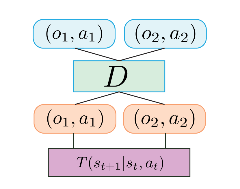
(a) Centralized (Cooperative)

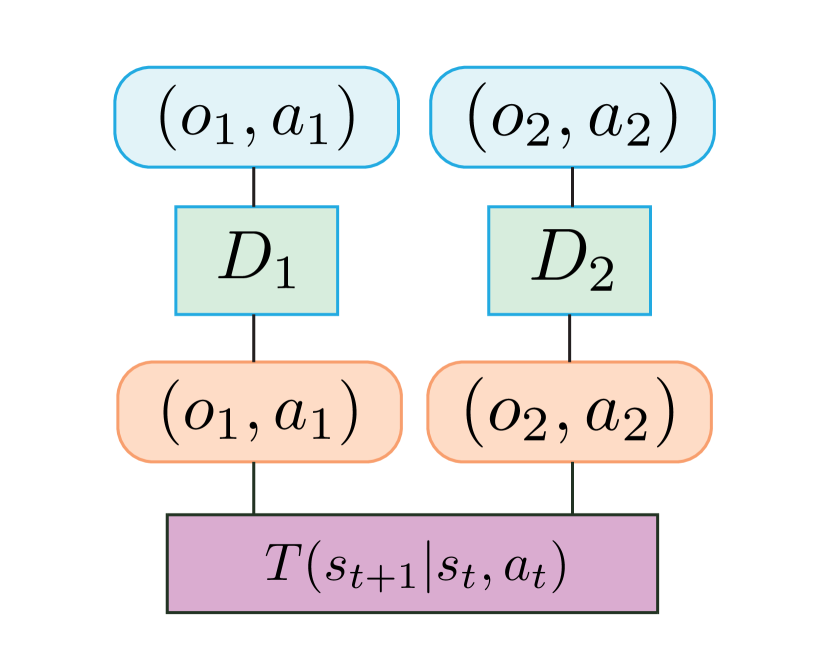
(b) Decentralized (Mixed)

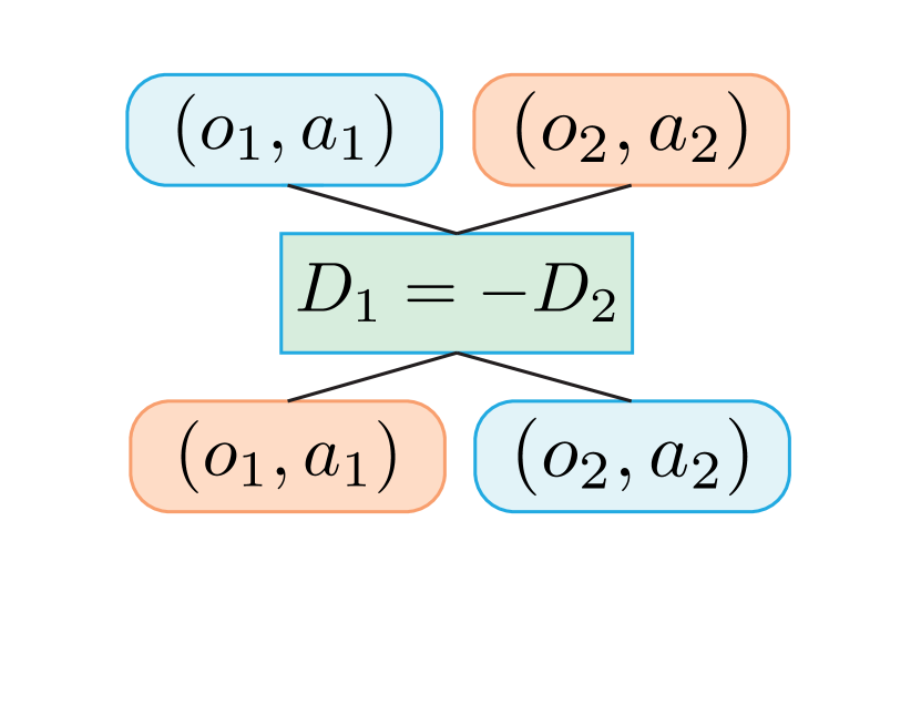
(c) Zero-sum (Competitive)

Figure 1: Different MAGAIL algorithms obtained with different priors on the reward structure. The discriminator tries to assign higher rewards to top row and low rewards to bottom row. In centralized and decentralized, the policy operates with the environment to match the expert rewards. In zero-sum, the policy do not interact with the environment; expert and policy trajectories are paired together as input to the discriminator.

These three settings are in summarized in Figure 1.

4.2 Multi-agent actor-critic with Kronecker factors

To optimize over the generator parameters $\theta$ in Eq. (11) we wish to use an algorithm for multi-agent RL that has good sample efficiency in practice. Our algorithm, which we refer to as Multi-agent Actor-Critic with Kronecker-factors (MACK), is based on Actor-Critic with Kronecker-factored Trust Region (ACKTR, (Wu et al., 2017)), a state-of-the-art natural policy gradient (Amari, 1998; Kakade, 2002) method in deep RL. MACK uses the framework of centralized training with decentralized execution (Foerster et al., 2016); policies are trained with additional information to reduce variance but such information is not used during execution time. We let the advantage function of every agent agent be a function of all agents’ observations and actions:

$$A_{\phi_{i}}^{\pi_{i}}(s,a_{t})=\sum_{j=0}^{k-1} (\gamma^{j}r(s_{t+j},a_{t+j})+\gamma^{k}V_{\phi_{i}}^{\pi_{i}}(s_{t+k},a_{-i,t}))V_{\phi_{i}}^{\pi_{i}}(s_{t},a_{-i,t})$$ (12)

where $V_{\phi_{i}}^{\pi_{i}}(s_{k},a_{-i})$ is the baseline for $i$, utilizing the additional information $(a_{-i})$ for variance reduction. We use (approximated) natural policy gradients to update both $\theta$ and $\phi$ but without trust regions to schedule the learning rate – a linear decay learning rate schedule achieves similar empirical performance.

MACK has some notable differences from Multi-Agent Deep Deterministic Policy Gradient (Lowe et al., 2017). On the one hand, MACK does not assume knowledge of other agent’s policies nor tries to infer them; the value estimator merely collects experience from other agents (and treats them as black boxes). On the other hand, MACK does not require gradient estimators such as Gumbel-softmax (Jang et al., 2016; Maddison et al., 2016) to optimize over discrete actions, which is necessary for DDPG (Lillicrap et al., 2015).

5 Experiments

We evaluate the performance of (centralized, decentralized, and zero-sum versions) of MAGAIL under two types of environments. One is a particle environment which allows for complex interactions and behaviors; the other is a control task, where multiple agents try to cooperate and move a plank forward. We collect results by averaging over 5 random seeds. Our implementation is based on OpenAI baselines (Dhariwal et al., 2017); please refer to Appendix C for implementation details.

We compare our methods (centralized, decentralized, zero-sum MAGAIL) with two baselines. The first is behavior cloning (BC), which learns a maximum likelihood estimate for $a_{i}$ given each state $s$ and does not require actions from other agents. The second baseline is the GAIL IRL baseline that operates on each agent separately – for each agent we first pretrain the other agents with BC, and then train the agent with GAIL; we then gather the trained GAIL policies from all the agents and evaluate their performance.

5.1 Particle environments

We first consider the particle environment proposed in (Lowe et al., 2017), which consists of several agents and landmarks. We consider two cooperative environments and two competitive ones. All environments have an underlying true reward function that allows us to evaluate the performance of learned agents.

The environments include: Cooperative Communication – two agents must cooperate to reach one of three colored landmarks. One agent (“speaker”) knows the goal but cannot move, so it must convey the message to the other agent (“listener”) that moves but does not observe the goal. Cooperative Navigation – three agents must cooperate through physical actions to reach three landmarks; ideally, each agent should cover a single landmark. Keep-Away – two agents have contradictory goals, where agent 1 tries to reach one of the two targeted landmarks, while agent 2 (the adversary) tries to keep agent 1 from reaching its target. The adversary does not observe the target, so it must act based on agent 1’s actions. Predator-Prey – three slower cooperating adversaries must chase the faster agent in a randomly generated environment with obstacles; the adversaries are rewarded by touching the agent while the agent is penalized.

For the cooperative tasks, we use an analytic expression defining the expert policy; for the competitive tasks, we use MACK to train expert policies based on the true underlying rewards (using larger policy and value networks than the ones that we use for imitation). We then use the expert policies to simulate trajectories $\mathcal{D}$, and then do imitation learning on $\mathcal{D}$ as demonstrations, where we assume the underlying rewards are unknown. Following (Li et al., 2017), we pretrain our Multi-Agent GAIL methods and the GAIL baseline using behavior cloning as initialization to reduce sample complexity for exploration. We consider 100 to 400 episodes of expert demonstrations, each with 50 timesteps, which is close to the amount of timesteps used for the control tasks in Ho and Ermon (2016). Moreover, we randomly sample the starting position of agent and landmarks each episode, so our policies have to learn to generalize when they encounter new settings.

5.1.1 Cooperative tasks

We evaluate performance in cooperative tasks via the average expected reward obtained by all the agents in an episode. In this environment, the starting state is randomly initialized, so generalization is crucial. We do not consider the zero-sum case, since it violates the cooperative nature of the task. We display the performance of centralized, decentralized, GAIL and BC in Figure 2.

Naturally, the performance of BC and MAGAIL increases with more expert demonstrations. MAGAIL performs consistently better than BC in all the settings; interestingly, in the cooperative communication task, centralized MAGAIL is able to achieve expert-level performance with only 200 demonstrations, but BC fails to come close even with 400 trajectories. Moreover, the centralized MAGAIL performs slightly better than decentralized MAGAIL due to the better prior, but decentralized MAGAIL still learns a highly correlated reward between two agents.

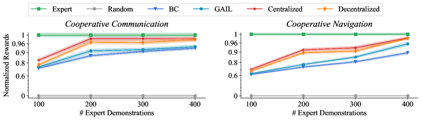
Figure 2: Average true reward from cooperative tasks. Performance of experts and random policies are normalized to one and zero respectively. We use inverse log scale for better comparison.

Table 1: Average agent rewards in competitive tasks. We compare behavior cloning (BC), GAIL (G), Centralized (C), Decentralized (D), and Zero-Sum (ZS) methods. Best marked in bold (high vs. low rewards is preferable depending on the agent vs. adversary role).

Task	Predator-Prey
Agent	Behavior Cloning					G	C	D	ZS
Adversary	BC	G	C	D	ZS	Behavior Cloning
Rewards	-93.20	-93.71	-93.75	-95.22	-95.48	-90.55	-91.36	-85.00	-89.4
Task	Keep-Away
Agent	Behavior Cloning					G	C	D	ZS
Adversary	BC	G	C	D	ZS	Behavior Cloning
Rewards	24.22	24.04	23.28	23.56	23.19	26.22	26.61	28.73	27.80

5.1.2 Competitive tasks

We consider all three types of Multi-Agent GAIL (centralized, decentralized, zero-sum) and BC in both competitive tasks. Since there are two opposing sides, it is hard to measure performance directly. Therefore, we compare by letting (agents trained by) BC play against (adversaries trained by) other methods, and vice versa. From Table 1, decentralized and zero-sum MAGAIL often perform better than centralized MAGAIL and BC, which suggests that the selection of the suitable prior $\hat{\psi}$ is important for good empirical performance. More details for all the particle environments are in the appendix.

5.2 Cooperative control

In some cases we are presented with sub-optimal expert demonstrations because the environment has changed; we consider this case in a cooperative control task (K. Gupta and Egorov, 2017), where $N$ bipedal walkers cooperate to move a long plank forward; the agents have incentive to collaborate since the plank is much longer than any of the agents. The expert demonstrates its policy on an environment with no bumps on the ground and heavy weights, while we perform imitation in an new environment with bumps and lighter weights (so one is likely to use too much force). Agents trained with BC tend to act more aggressively and fail, whereas agents trained with centralized MAGAIL can adapt to the new environment. With 10 (imperfect) expert demonstrations, BC agents have a chance of failure of $39.8\%$ (with a reward of 1.26), while centralized MAGAIL agents fail only $26.2\%$ of the time (with a reward of 26.57). We show videos of respective policies in the supplementary.

6 Related work and discussion

There is a vast literature on single-agent imitation learning (Bagnell, 2015). Behavior Cloning (BC) learns the policy through supervised learning (Pomerleau, 1991). Inverse Reinforcement Learning (IRL) assumes the expert policy optimizes over some unknown reward, recovers the reward, and learns the policy through reinforcement learning (RL). BC does not require knowledge of transition probabilities or access to the environment, but suffers from compounding errors and covariate shift (Ross and Bagnell, 2010; Ross et al., 2011).

Most existing work in multi-agent imitation learning assumes the agents have very specific reward structures. The most common case is fully cooperative agents, where the challenges mainly lie in other factors, such as unknown role assignments (Le et al., 2017), scalability to swarm systems (Šošic et al., 2016) and agents with partial observations (Bogert and Doshi, 2014). In non-cooperative settings,  Lin et al. (2014) consider the case of IRL for two-player zero-sum games and cast the IRL problem as Bayesian inference, while Reddy et al. (2012) assume agents are non-cooperative but the reward function is a linear combination of pre-specified features.

Our work is the first to propose a general multi-agent IRL framework that bridges the gap between state-of-the art multi-agent reinforcement learning methods (Lowe et al., 2017; Foerster et al., 2016) and implicit generative models such as generative adversarial networks (Goodfellow et al., 2014). Experimental results demonstrate that it is able to imitate complex behaviors in high-dimensional environments with both cooperative and adversarial interactions. An interesting research direction is to explore new techniques for gathering expert demonstration; for example, when the expert is allowed to aid the agents by participating in part of the agent’s learning process (Hadfield-Menell et al., 2016).

A Proofs

We use ${{\hat{v}}}_{i}(s)$, ${{\hat{q}}}_{i}(s,a_{i})$ and $Q(\tau)$ to represent ${{\hat{v}}}_{i}(s;{\bm{\pi}},{{\bf r}})$, ${{\hat{q}}}_{i}(s,a_{i};{\bm{\pi}},{{\bf r}})$ and $Q(\tau;{\bm{\pi}},{{\bf r}})$, where we implicitly assume dependency over ${\bm{\pi}}$ and ${{\bf r}}$.

A.1 Proof to Lemma 8

For any policy ${\bm{\pi}}$, $f_{{\bf r}}({\bm{\pi}},{{\hat{v}}})=0$ when ${{\hat{v}}}$ is the value function of ${\bm{\pi}}$ (due to Bellman equations). However, only policies that form a Nash equilibrium satisfies the constraints in Eq. 2; we formalize this in the following Lemma.

Lemma 8

Let ${{\hat{v}}}_{i}(s;{\bm{\pi}},{{\bf r}})$ be the solution to the Bellman equation

$${{\hat{v}}}_{i}(s)=\mathbb{E}_{{\bm{\pi}}}[r_{i}(s,{{\bf a}})+\gamma\sum_{s^{\prime}\in\mathcal{S}}T(s^{\prime}|s,{{\bf a}}){{\hat{v}}}_{i}(s^{\prime})]$$

and ${{\hat{q}}}_{i}(s,a_{i})=\mathbb{E}_{\pi_{-i}}[r_{i}(s,{{\bf a}})+\gamma\sum_{s^{\prime}\in\mathcal{S}}T(s^{\prime}|s,{{\bf a}}){{\hat{v}}}_{i}(s^{\prime})]$. Then for any $\pi$,

$$f_{{\bf r}}({\bm{\pi}},{{\hat{v}}}({\bm{\pi}}))=0$$

Furthermore, ${\bm{\pi}}$ is Nash equilibrium under $r$ if and only if ${{\hat{v}}}_{i}(s)\geq{{\hat{q}}}_{i}(s,a_{i})$ for all $i\in[N],s\in\mathcal{S},a_{i}\in\mathcal{A}_{i}$.

Proof  By definition of ${{\hat{v}}}_{i}(s)$ we have:

$${{\hat{v}}}_{i}(s) =\mathbb{E}_{{\bm{\pi}}}[r_{i}(s,{{\bf a}})+\gamma\sum_{s^{\prime}\in\mathcal{S}}T(s^{\prime}|s,{{\bf a}}){{\hat{v}}}_{i}(s^{\prime})]$$

$$=\mathbb{E}_{\pi_{i}}\mathbb{E}_{\pi_{-i}}[r_{i}(s,{{\bf a}})+\gamma\sum_{s^{\prime}\in\mathcal{S}}T(s^{\prime}|s,{{\bf a}}){{\hat{v}}}_{i}(s^{\prime})]$$

$$=\mathbb{E}_{\pi_{i}}[{{\hat{q}}}_{i}(s,a_{i})]$$

which uses the fact that $a_{i}$ and $a_{-i}$ are independent conditioned on $s$. Hence $f_{{\bf r}}({\bm{\pi}},{{\hat{v}}})=0$ immediately follows.

If ${\bm{\pi}}$ is a Nash equilibrium, and at least one of the constrains does not hold, i.e. there exists some $i$ and $s,a_{i}$ such that ${{\hat{v}}}(s)<{{\hat{q}}}(s,a_{i})$, then agent $i$ can achieve a strictly higher expected return if it chooses to take actions $a_{i}$ whenever it encounters state $s_{i}$ and follow $\pi_{i}$ for rest of the states, which violates the Nash equilibrium assumption.

If the constraints hold, i.e. for all $i$ and $(s,a_{i})$, ${{\hat{v}}}_{i}(s)\geq{{\hat{q}}}_{i}(s,a_{i})$ then

$${{\hat{v}}}_{i}(s)\geq\mathbb{E}_{\pi_{i}}[{{\hat{q}}}_{i}(s,a_{i})]={{\hat{v}}}_{i}(s)$$

so value iteration over ${{\hat{v}}}_{i}(s)$ converges. If we can find another policy ${\bm{\pi}}^{\prime}$ such that ${{\hat{v}}}_{i}(s)<\mathbb{E}_{\pi^{\prime}_{i}}[{{\hat{q}}}_{i}(s,a_{i})]$, then there should be at least one violation in the constraints since $\pi^{\prime}_{i}$ must be a convex combination (expectation) over actions $a_{i}$. Therefore, for any policy $\pi_{i}^{\prime}$ and action $a_{i}$ for any agent $i$, $\mathbb{E}_{\pi_{i}}[{{\hat{q}}}_{i}(s,a_{i})]\geq\mathbb{E}_{\pi_{i}^{\prime}}[{{\hat{q}}}_{i}(s,a_{i})]$ always hold, so $\pi_{i}$ is the optimal response to $\pi_{-i}$, and $\pi$ constitutes a Nash equilibrium when we repeat this argument for all agents.

Notably, Theorem 3.8.2 in Filar and Vrieze (2012) discusses the equivalence by assuming $f_{{\bf r}}({\bm{\pi}},v)=0$ for some $v$; if $v$ satisfies the assumptions, then $v={{\hat{v}}}^{\prime}$.  

A.2 Proof to Theorem 3

Proof  If $\pi$ is a Nash equilibrium, and at least one of the constraints does not hold, i.e. there exists some $i$ and $\{s^{(j)},a_{i}^{(j)}\}_{j=0}^{t}$, such that

$${{\hat{v}}}_{i}(s^{(0)})<\mathbb{E}_{\pi_{-i}}[{{\hat{q}}}_{i}^{(t)}(\{s^{(j)},{{\bf a}}^{(j)}\}_{j=0}^{t-1},s^{(t)},a^{(t)}_{i})]$$

Then agent $i$ can achieve a strictly higher expected return on its own if it chooses a particular sequence of actions by taking $a_{i}^{(j)}$ whenever it encounters state $s^{(j)}$, and follow $\pi_{i}$ for the remaining states. We note that this is in expectation over the policy of other agents. Hence, we construct a policy for agent $i$ that has strictly higher value than $\pi_{i}$ without modifying $\pi_{-i}$, which contradicts the definition of Nash equilibrium.

If the constraints hold, i.e for all $i$ and $\{s^{(j)},a_{i}^{(j)}\}_{j=0}^{t}$,

$${{\hat{v}}}_{i}(s^{(0)})\geq\mathbb{E}_{\pi_{-i}}[{{\hat{q}}}_{i}^{(t)}(\{s^{(j)},{{\bf a}}^{(j)}\}_{j=0}^{t-1},s^{(t)},a^{(t)}_{i})]$$

then we can construct any ${{\hat{q}}}_{i}(s^{(0)},a_{i}^{(0)})$ via a convex combination by taking the expectation over $\pi_{i}$:

$${{\hat{q}}}_{i}(s^{(0)},a_{i}^{(0)})=\mathbb{E}_{\pi_{i}}[\mathbb{E}_{\pi_{-i}}[{{\hat{q}}}_{i}^{(t)}(\{s^{(j)},{{\bf a}}^{(j)}\}_{j=0}^{t-1},s^{(t)},a^{(t)}_{i})]]$$

where the expectation over $\pi_{i}$ is taken over actions $\{a_{i}^{(j)}\}_{j=0}^{t}$ (the expectation over states are contained in the inner expectation over $\pi_{-i}$). Therefore, $\forall i\in[N],s\in\mathcal{S},a_{i}\in\mathcal{A}_{i}$,

$${{\hat{v}}}_{i}(s)\geq{{\hat{q}}}_{i}(s,a_{i})$$

and we recover the constraints in Eq. 2. By Lemma 8, $\pi$ is a Nash equilibrium.  

A.3 Proof to Theorem 4

Proof  We use $Q^{\star},{{\hat{q}}}^{\star},{{\hat{v}}}^{\star}$ to denote the $Q$, ${{\hat{q}}}$ and ${{\hat{v}}}$ quantities defined for policy ${\bm{\pi}}^{\star}$. For the two terms in $L_{r}^{(t+1)}({\bm{\pi}}^{\star},\lambda_{\bm{\pi}}^{\star})$ we have:

$$L_{r}^{(t+1)}({\bm{\pi}}^{\star},\lambda_{\bm{\pi}}^{\star})=\sum_{i=1}^{N}\sum_{\tau_{i}\in\mathcal{T}_{i}}\lambda^{\star}(\tau_{i})(Q_{i}^{\star}(\tau_{i})-{{\hat{v}}}_{i}^{\star}(s^{(0)}))$$ (13)

For any agent $i$, we note that

$$\sum_{\tau_{i}\in\mathcal{T}_{i}}\lambda^{\star}(\tau_{i})Q_{i}^{\star}(\tau_{i})=\mathbb{E}_{\pi_{i}}\mathbb{E}_{\pi^{\star}_{-i}}[\sum_{j=0}^{t-1}\gamma^{j}r_{i}(s^{(j)},a^{(j)})+\gamma^{t}{{\hat{q}}}_{i}^{\star}(s^{t},a_{i}^{(t)})]$$

which amounts to using $\pi_{i}$ for agent $i$ for the first $t$ steps and using $\pi^{\star}_{i}$ for the remaining steps, whereas other agents follow $\pi^{\star}_{-i}$. As $t\to\infty$, this converges to $\mathbb{E}_{\pi_{i},\pi^{\star}_{-i}}[r_{i}]$ since $\gamma^{t}\to 0$ and $q^{\star}_{i}(s^{(t)},a_{i}^{(t)})$ is bounded. Moreover, for ${{\hat{v}}}^{\star}_{i}(s^{(0)})$, we have

$$\sum_{\tau_{i}\in\mathcal{T}_{i}}\lambda^{\star}(\tau_{i}){{\hat{v}}}^{\star}_{i}(s^{(0)})=\mathbb{E}_{s^{(0)}\sim\eta}[{{\hat{v}}}^{\star}_{i}(s^{(0)})]=\mathbb{E}_{{\bm{\pi}}^{\star}}[r_{i}]$$

Combining the two we have

$$L_{r}^{(t+1)}({\bm{\pi}}^{\star},\lambda^{\star}_{\bm{\pi}})=\sum_{i=1}^{N}\mathbb{E}_{\pi_{i},\pi^{\star}_{-i}}[r_{i}]-\sum_{i=1}^{N}\mathbb{E}_{{\bm{\pi}}^{\star}}[r_{i}]$$

which describes the differences in expected rewards.  

A.4 Proof to Theorem 6

Proof  Define the “MARL” objective for a single agent $i$ where other agents have policy $\pi_{E_{i}}$:

$$\mbox{MARL}_{i}(r_{i})=\max_{\pi_{i}}H_{i}(\pi_{i})+\mathbb{E}_{\pi_{i},\pi_{E_{-i}}}[r_{i}]$$

Define the “MAIRL” objective for a single agent $i$ where other agents have policy $\pi_{E}$:

$$\mbox{MAIRL}_{i,\psi}(\pi^{\star})=\operatorname*{arg\,max}_{r_{i}}\psi_{i}(r_{i})+\mathbb{E}_{\pi_{E}}[r_{i}]-(\max_{\pi_{i}}H_{i}(\pi_{i})+\mathbb{E}_{\pi_{i},\pi_{E_{-i}}}[r_{i}])$$

Since $r_{i}$ and $\pi_{i}$’s are independent in the MAIRL objective, the solution to $\mbox{MAIRL}_{\psi}$ can be represented by the solutions of $\mbox{MAIRL}_{i,\psi}$ for each $i$:

$$\mbox{MAIRL}_{\psi}=[\mbox{MAIRL}_{1,\psi},\ldots,\mbox{MAIRL}_{N,\psi}]$$

Moreover, the single agent “MARL” objective $\mbox{MARL}_{i}(r_{i})$ has a unique solution $\pi_{E_{i}}$, which also composes the (unique) solution to MARL (which we assumed in Section 3. Therefore,

$$\mbox{MARL}({{\bf r}})=[\mbox{MARL}_{1}(r_{1}),\ldots,\mbox{MARL}_{N}(r_{N})]$$

So we can use Proposition 3.1 in Ho and Ermon (2016) for each agent $i$ with $\mbox{MARL}_{i}(r_{i})$ and $\mbox{MAIRL}_{i,\psi}(\pi^{\star})$ and achieve the same solution as $\mbox{MARL}\circ\mbox{MAIRL}_{\psi}$.  

A.5 Proof to Proposition 7

Proof  From Corollary A.1.1 in Ho and Ermon (2016), we have

$$\psi^{\star}_{GA}(\rho_{\bm{\pi}}-\rho_{{\bm{\pi}}_{E}})=\max_{D\in(0,1)^{\mathcal{S}\times\mathcal{A}}}\mathbb{E}_{{\bm{\pi}}}[\log D(s,a)]+\mathbb{E}_{{\bm{\pi}}_{E}}[\log(1-D(s,a))]\equiv D_{JS}(\rho_{\bm{\pi}},\rho_{{\bm{\pi}}_{E}})$$

where $D_{JS}$ denotes Jensen-Shannon divergence (which is a squared metric), and $\equiv$ denotes equivalence up to shift and scaling.

Taking the min over this we obtain

$$\operatorname*{arg\,min}_{\pi}\sum_{i=1}^{N}\psi^{\star}_{GA}(\rho_{\pi}-\rho_{{\bm{\pi}}_{E}})={\bm{\pi}}_{E}$$

Similarly,

$$\operatorname*{arg\,min}_{\pi}\sum_{i=1}^{N}\psi^{\star}_{GA}(\rho_{\pi_{i},\pi_{E_{-i}}}-\rho_{{\bm{\pi}}_{E}})={\bm{\pi}}_{E}$$

So these two quantities are equal.  

B MAGAIL Algorithm

We include the MAGAIL algorithm as follows:

Algorithm 1 Multi-Agent GAIL (MAGAIL)

  Input: Initial parameters of policies, discriminators and value (baseline) estimators $\theta_{0},\omega_{0}$, $\phi_{0}$; expert trajectories $\mathcal{D}=\{(s_{j},a_{j})\}_{j=0}^{M}$; batch size $B$; Markov game as a black box $(N,\mathcal{S},\mathcal{A},\eta,T,r,{{\bf o}},\gamma)$.

  Output: Learned policies $\pi_{\theta}$ and reward functions $D_{\omega}$.

  for $u=0,1,2,\ldots$ do

     Obtain trajectories of size $B$ from $\pi$ by the process: $s_{0}\sim\eta(s),a_{t}\sim\pi_{\theta_{u}}(a_{t}|s_{t}),s_{t+1}\sim T(s_{t}|a_{t})$.

     Sample state-action pairs from $\mathcal{D}$ with batch size $B$.

     Denote state-action pairs from $\pi$ and $\mathcal{D}$ as $\chi$ and $\chi_{E}$.

     for $i=1,\ldots,n$ do

        Update $\omega_{i}$ to increase the objective

$$\mathbb{E}_{\chi}[\log D_{\omega_{i}}(s,a_{i})]+\mathbb{E}_{\chi_{E}}[\log(1-D_{\omega_{i}}(s,a_{i}))]$$

     end for

     for $i=1,\ldots,n$ do

        Compute value estimate $V^{\star}$ and advantage estimate $A_{i}$ for $(s,a)\in\chi$.

        Update $\phi_{i}$ to decrease the objective

$$\mathbb{E}_{\chi}[(V_{\phi}(s,a_{-i})-V^{\star}(s,a_{-i}))^{2}]$$

        Update $\theta_{i}$ by policy gradient with small step sizes:

$$\mathbb{E}_{\chi}[\nabla_{\theta_{i}}\pi_{\theta_{i}}(a_{i}|o_{i})A_{i}(s,a)]$$

     end for

  end for

C Experiment Details

C.1 Hyperparameters

For the particle environment, we use two layer MLPs with 128 cells in each layer, for the policy generator network, value network and the discriminator. We use a batch size of 1000. The policy is trained using K-FAC optimizer (Martens and Grosse, 2015) with learning rate of 0.1. All other parameters for K-FAC optimizer are the same in (Wu et al., 2017).

For the cooperative control task, we use two layer MLPs with 64 cells in each layer for all the networks. We use a batch size of 2048, and learning rate of 0.03. We obtain expert trajectories by training the expert with MACK and sampling demonstrations from the same environment. Hence, the expert’s demonstrations are imperfect (or even flawed) in the environment that we test on.

Table 2: Performance in cooperative navigation.

# Expert Episodes	100	200	300	400
Expert	-13.50 $\pm$ 6.3
Random	-128.13 $\pm$ 32.1
Behavior Cloning	-56.82 $\pm$ 18.9	-43.10 $\pm$ 16.0	-35.66 $\pm$ 15.2	-25.83 $\pm$ 12.7
Centralized	-46.66 $\pm$ 20.8	-23.10 $\pm$ 12.4	-21.53 $\pm$ 12.9	-15.30 $\pm$ 7.0
Decentralized	-50.00 $\pm$ 18.6	-25.61 $\pm$ 12.3	-24.10 $\pm$ 13.3	-15.55 $\pm$ 6.5
GAIL	-55.01 $\pm$ 17.7	-39.21 $\pm$ 16.5	-29.89 $\pm$ 13.5	-18.76 $\pm$ 12.1

Table 3: Performance in cooperative communication.

# Expert Episodes	100	200	300	400
Expert	-6.22 $\pm$ 4.5
Random	-62.49 $\pm$ 28.7
Behavior Cloning	-21.25 $\pm$ 10.6	-13.25 $\pm$ 7.4	-11.37 $\pm$ 5.9	-10.00 $\pm$ 5.36
Centralized	-15.65 $\pm$ 10.0	-7.11 $\pm$ 4.8	-7.11 $\pm$ 4.8	-7.09 $\pm$ 4.8
Decentralized	-18.68 $\pm$ 10.4	-8.06 $\pm$ 5.3	-8.16 $\pm$ 5.5	-7.34 $\pm$ 4.9
GAIL	-20.28 $\pm$ 10.1	-11.06 $\pm$ 7.8	-10.51 $\pm$ 6.6	-9.44 $\pm$ 5.7

C.2 Detailed Results

We use the particle environment introduced in (Lowe et al., 2017) and the multi-agent control environment (K. Gupta and Egorov, 2017) for experiments. We list the exact performance in Tables 2, 3 for cooperative tasks, and Table 4 and competitive tasks. The means and standard deviations are computed over 100 episodes. The policies in the cooperative tasks are trained with varying number of expert demonstrations. The policies in the competitive tasks are trained with on a dataset with 100 expert trajectories.

The environment for each episode is drastically different (e.g. location of landmarks are randomly sampled), which leads to the seemingly high standrad deviation across episodes.

Table 4: Performance in competitive tasks.

Task	Agent Policy	Adversary Policy	Agent Reward
Predator-Prey	Behavior Cloning	Behavior Cloning	-93.20 $\pm$ 63.7
		GAIL	-93.71 $\pm$ 64.2
		Centralized	-93.75 $\pm$ 61.9
		Decentralized	-95.22 $\pm$ 49.7
		Zero-Sum	-95.48 $\pm$ 50.4
	GAIL	Behavior Cloning	-90.55 $\pm$ 63.7
	Centralized		-91.36 $\pm$ 58.7
	Decentralized		-85.00 $\pm$ 42.3
	Zero-Sum		-89.4 $\pm$ 48.2
Keep-Away	Behavior Cloning	Behavior Cloning	24.22 $\pm$ 21.1
		GAIL	24.04 $\pm$ 18.2
		Centralized	23.28 $\pm$ 20.6
		Decentralized	23.56 $\pm$ 19.9
		Zero-Sum	23.19 $\pm$ 19.9
	GAIL	Behavior Cloning	26.22 $\pm$ 19.1
	Centralized		26.61 $\pm$ 20.0
	Decentralized		28.73 $\pm$ 18.3
	Zero-Sum		27.80 $\pm$ 19.2

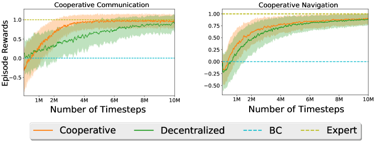
Figure 3: Sample complexity of multi-agent GAIL methods under cooperative tasks. Performance of experts is normalized to one, and performance of behavior cloning is normalized to zero. The standard deviation is computed with respect to episodes, and is noisy due to randomness in the environment.

C.3 Video Demonstrations

We show certain trajectories generated by our methods. The vidoes are here: videos.

For the particle case:

Navigation-BC-Agents.gif

Agents trained by behavior cloning in the navigation task.

Navigation-GAIL-Agents.gif

Agents trained by proposed framework in the navigation task.

Predator-Prey-BC-Agent-BC-Adversary.gif

Agent (green) trained by behavior cloning play against adversaries (red) trained by behavior cloning.

Predator-Prey-GAIL-Agent-BC-Adversary.gif

Agent (green) trained by proposed framework play against adversaries (red) trained by behavior cloning.

For the cooperative control case:

Multi-Walker-Expert.mp4

Expert demonstrations in the “easy” environment.

Multi-Walker-GAIL.mp4

Centralized GAIL trained on the “hard” environment.

Multi-Walker-BC.mp4

BC trained on the “hard” environment.

Interestingly, the failure modes for the agents in “hard” environment is mostly having the plank fall off or bounce off, since by decreasing the weight of the plank will decrease its friction force and increase its acceleration.

References

- Abbeel and Ng (2004) Pieter Abbeel and Andrew Y Ng. Apprenticeship learning via inverse reinforcement learning. In Proceedings of the twenty-first international conference on Machine learning, page 1. ACM, 2004.
- Amari (1998) Shun-Ichi Amari. Natural gradient works efficiently in learning. Neural computation, 10(2):251–276, 1998.
- Amodei and Clark (2016) Dario Amodei and Jack Clark. Faulty reward functions in the wild, 2016.
- Amodei et al. (2016) Dario Amodei, Chris Olah, Jacob Steinhardt, Paul Christiano, John Schulman, and Dan Mané. Concrete problems in ai safety. arXiv preprint arXiv:1606.06565, 2016.
- Bagnell (2015) J Andrew Bagnell. An invitation to imitation. Technical report, CARNEGIE-MELLON UNIV PITTSBURGH PA ROBOTICS INST, 2015.
- Bloem and Bambos (2014) Michael Bloem and Nicholas Bambos. Infinite time horizon maximum causal entropy inverse reinforcement learning. In Decision and Control (CDC), 2014 IEEE 53rd Annual Conference on, pages 4911–4916. IEEE, 2014.
- Bogert and Doshi (2014) Kenneth Bogert and Prashant Doshi. Multi-robot inverse reinforcement learning under occlusion with interactions. In Proceedings of the 2014 international conference on Autonomous agents and multi-agent systems, pages 173–180. International Foundation for Autonomous Agents and Multiagent Systems, 2014.
- Dhariwal et al. (2017) Prafulla Dhariwal, Christopher Hesse, Oleg Klimov, Alex Nichol, Matthias Plappert, Alec Radford, John Schulman, Szymon Sidor, and Yuhuai Wu. Openai baselines. https://github.com/openai/baselines, 2017.
- Englert and Toussaint (2015) Peter Englert and Marc Toussaint. Inverse kkt–learning cost functions of manipulation tasks from demonstrations. In Proceedings of the International Symposium of Robotics Research, 2015.
- Espeholt et al. (2018) Lasse Espeholt, Hubert Soyer, Remi Munos, Karen Simonyan, Volodymir Mnih, Tom Ward, Yotam Doron, Vlad Firoiu, Tim Harley, Iain Dunning, Shane Legg, and Koray Kavukcuoglu. Impala: Scalable distributed deep-rl with importance weighted actor-learner architectures. arXiv preprint arXiv:1802.01561, 2018.
- Filar and Vrieze (2012) Jerzy Filar and Koos Vrieze. Competitive Markov decision processes. Springer Science & Business Media, 2012.
- Finn et al. (2016) Chelsea Finn, Sergey Levine, and Pieter Abbeel. Guided cost learning: Deep inverse optimal control via policy optimization. In International Conference on Machine Learning, pages 49–58, 2016.
- Foerster et al. (2016) Jakob Foerster, Yannis Assael, Nando de Freitas, and Shimon Whiteson. Learning to communicate with deep multi-agent reinforcement learning. In Advances in Neural Information Processing Systems, pages 2137–2145, 2016.
- Goodfellow et al. (2014) Ian Goodfellow, Jean Pouget-Abadie, Mehdi Mirza, Bing Xu, David Warde-Farley, Sherjil Ozair, Aaron Courville, and Yoshua Bengio. Generative adversarial nets. In Advances in neural information processing systems, pages 2672–2680, 2014.
- Hadfield-Menell et al. (2016) Dylan Hadfield-Menell, Stuart J Russell, Pieter Abbeel, and Anca Dragan. Cooperative inverse reinforcement learning. In Advances in neural information processing systems, pages 3909–3917, 2016.
- Hadfield-Menell et al. (2017) Dylan Hadfield-Menell, Smitha Milli, Pieter Abbeel, Stuart J Russell, and Anca Dragan. Inverse reward design. In Advances in Neural Information Processing Systems, pages 6768–6777, 2017.
- Ho and Ermon (2016) Jonathan Ho and Stefano Ermon. Generative adversarial imitation learning. In Advances in Neural Information Processing Systems, pages 4565–4573, 2016.
- Hu et al. (1998) Junling Hu, Michael P Wellman, et al. Multiagent reinforcement learning: theoretical framework and an algorithm. In ICML, volume 98, pages 242–250. Citeseer, 1998.
- Jang et al. (2016) Eric Jang, Shixiang Gu, and Ben Poole. Categorical reparameterization with gumbel-softmax. arXiv preprint arXiv:1611.01144, 2016.
- K. Gupta and Egorov (2017) Jayesh K. Gupta and Maxim Egorov. Multi-agent deep reinforcement learning environment. https://github.com/sisl/madrl, 2017.
- Kakade (2002) Sham M Kakade. A natural policy gradient. In Advances in neural information processing systems, pages 1531–1538, 2002.
- Le et al. (2017) Hoang M Le, Yisong Yue, and Peter Carr. Coordinated multi-agent imitation learning. arXiv preprint arXiv:1703.03121, 2017.
- Leibo et al. (2017) Joel Z Leibo, Vinicius Zambaldi, Marc Lanctot, Janusz Marecki, and Thore Graepel. Multi-agent reinforcement learning in sequential social dilemmas. In Proceedings of the 16th Conference on Autonomous Agents and MultiAgent Systems, pages 464–473. International Foundation for Autonomous Agents and Multiagent Systems, 2017.
- Li et al. (2017) Yunzhu Li, Jiaming Song, and Stefano Ermon. Infogail: Interpretable imitation learning from visual demonstrations. arXiv preprint arXiv:1703.08840, 2017.
- Lillicrap et al. (2015) Timothy P Lillicrap, Jonathan J Hunt, Alexander Pritzel, Nicolas Heess, Tom Erez, Yuval Tassa, David Silver, and Daan Wierstra. Continuous control with deep reinforcement learning. arXiv preprint arXiv:1509.02971, 2015.
- Lin et al. (2014) Xiaomin Lin, Peter A Beling, and Randy Cogill. Multi-agent inverse reinforcement learning for zero-sum games. arXiv preprint arXiv:1403.6508, 2014.
- Littman (1994) Michael L Littman. Markov games as a framework for multi-agent reinforcement learning. In Proceedings of the eleventh international conference on machine learning, volume 157, pages 157–163, 1994.
- Lowe et al. (2017) Ryan Lowe, Yi Wu, Aviv Tamar, Jean Harb, Pieter Abbeel, and Igor Mordatch. Multi-agent actor-critic for mixed cooperative-competitive environments. arXiv preprint arXiv:1706.02275, 2017.
- Maddison et al. (2016) Chris J Maddison, Andriy Mnih, and Yee Whye Teh. The concrete distribution: A continuous relaxation of discrete random variables. arXiv preprint arXiv:1611.00712, 2016.
- Martens and Grosse (2015) James Martens and Roger Grosse. Optimizing neural networks with kronecker-factored approximate curvature. In International Conference on Machine Learning, pages 2408–2417, 2015.
- Matignon et al. (2012) Laëtitia Matignon, Laurent Jeanpierre, Abdel-Illah Mouaddib, et al. Coordinated multi-robot exploration under communication constraints using decentralized markov decision processes. In AAAI, 2012.
- Ng et al. (2000) Andrew Y Ng, Stuart J Russell, et al. Algorithms for inverse reinforcement learning. In Icml, pages 663–670, 2000.
- Peng et al. (2017) Peng Peng, Quan Yuan, Ying Wen, Yaodong Yang, Zhenkun Tang, Haitao Long, and Jun Wang. Multiagent bidirectionally-coordinated nets for learning to play starcraft combat games. arXiv preprint arXiv:1703.10069, 2017.
- Pomerleau (1991) Dean A Pomerleau. Efficient training of artificial neural networks for autonomous navigation. Neural Computation, 3(1):88–97, 1991.
- Prasad and Bhatnagar (2015) HL Prasad and Shalabh Bhatnagar. A study of gradient descent schemes for general-sum stochastic games. arXiv preprint arXiv:1507.00093, 2015.
- Reddy et al. (2012) Tummalapalli Sudhamsh Reddy, Vamsikrishna Gopikrishna, Gergely Zaruba, and Manfred Huber. Inverse reinforcement learning for decentralized non-cooperative multiagent systems. In Systems, Man, and Cybernetics (SMC), 2012 IEEE International Conference on, pages 1930–1935. IEEE, 2012.
- Ross and Bagnell (2010) Stéphane Ross and Drew Bagnell. Efficient reductions for imitation learning. In AISTATS, pages 3–5, 2010.
- Ross et al. (2011) Stéphane Ross, Geoffrey J Gordon, and Drew Bagnell. A reduction of imitation learning and structured prediction to no-regret online learning. In AISTATS, page 6, 2011.
- Šošic et al. (2016) Adrian Šošic, Wasiur R KhudaBukhsh, Abdelhak M Zoubir, and Heinz Koeppl. Inverse reinforcement learning in swarm systems. stat, 1050:17, 2016.
- Stadie et al. (2017) Bradly Stadie, Pieter Abbeel, and Ilya Sutskever. Third person imitation learning. In ICLR, 2017.
- Sutton and Barto (1998) Richard S Sutton and Andrew G Barto. Reinforcement learning: An introduction, volume 1. MIT press Cambridge, 1998.
- Wu et al. (2017) Yuhuai Wu, Elman Mansimov, Roger B Grosse, Shun Liao, and Jimmy Ba. Scalable trust-region method for deep reinforcement learning using kronecker-factored approximation. In Advances in neural information processing systems, pages 5285–5294, 2017.
- Ziebart et al. (2008) Brian D Ziebart, Andrew L Maas, J Andrew Bagnell, and Anind K Dey. Maximum entropy inverse reinforcement learning. In AAAI, volume 8, pages 1433–1438. Chicago, IL, USA, 2008.