Towards the Theory of the Yukawa Potential

Abstract

Using three different approaches, Perturbation Theory (PT), the Lagrange Mesh Method (Lag-Mesh) and the Variational Method (VM), we study the low-lying states of the Yukawa potential $V(r)=-(\lambda/r)e^{-\alpha r}\,$. First orders in PT in powers of $\alpha$ are calculated in the framework of the Non-Linerization Procedure. It is found that the Padé approximants to PT series together with the Lag-Mesh provide highly accurate values of the energy and the positions of the radial nodes of the wave function. The most accurate results, at present, of the critical screening parameters ($\alpha_{c}$) for some low-lying states and the first coefficients in the expansion of the energy at $\alpha_{c}$ are presented. A locally-accurate and compact approximation for the eigenfunctions of the low-lying states for any $r\in[0,\infty)$ is discovered. This approximation used as a trial function in VM eventually leads to energies as precise as those of PT and Lag-Mesh. Finally, a compact analytical expression for the energy as a function of $\alpha$, that reproduce at least $6$ decimal digits in the entire physical range of $\alpha$, is found.

I Introduction

The Yukawa potential, sometimes called the screened Coulomb potential, has a wide range of applications in many branches of physics. Originally, Yukawa Yukawa proposed this potential to describe the interaction between a pair of nucleons. However, it is often used as a first approximation of the interaction between two dust particles immersed in a plasma Plasma1 ; Plasma2 ; Plasma3 . The interaction of dark matter particles through a Yukawa potential could explain the recently observed cores in dwarf galaxies Dark . The Yukawa potential has also been employed to model the systems of colloidal particles in electrolytes Colloidal .

In the standard form the three-dimensional Yukawa potential is given by

$$V(r)\ =\ -\lambda\,\frac{e^{-\alpha r}}{r}\ ,$$ (1)

where $\alpha\geq 0$ and $\lambda>0$ are parameters and $r$ is the radial coordinate. If $\alpha=0$, the Yukawa potential degenerates into the Coulomb potential. When $\alpha\rightarrow\infty$, the Yukawa potential vanishes: it describes a free motion.

In the non-relativistic approximation the radial Schrödinger equation (in atomic units $\hbar=m=1$) with the Yukawa potential (1) reads

$$\left[-\frac{1}{2}\,\frac{d^{2}}{dr^{2}}\ -\ \frac{1}{r}\,\frac{d}{dr}+\ \frac{l\,(l+1)}{2r^{2}}\ -\ \lambda\,\frac{e^{-\alpha r}}{r}\right]\Psi_{n,l}\ =\ E_{n,l}(\lambda,\alpha)\,\Psi_{n,l}\ ,$$ (2)

where $n=0$, $1$, $...,$ is the principal quantum number and $l=0$, $1$, …, $n-1,$ is the angular momentum. It is well known that the Schrödinger equation (2) with $\alpha\neq 0$ is not exactly solvable and only holds a finite number of bound states. Naturally, this number depends on the parameters $\alpha$ and $\lambda$. The scaling transformation $r\rightarrow\lambda^{-1}\,r$ in the equation (2) allow us to remove the $\lambda$ dependence of the energy since it is scaled as

$$E_{n,l}(\lambda,\alpha)\ =\ \lambda^{2}\,E_{n,l}(1,\alpha\,\lambda^{-1})\,.$$ (3)

From now on we set $\lambda=1$. Consequently the number of bound states as well as the energy $E_{n,l}$ depends only on the value of $\alpha$.

There is a certain critical value of $\alpha$, denoted by $\alpha_{c}^{(n,l)}$, with the following property: for $\alpha<\alpha_{c}^{(n,l)}$ the state $(n,l)$ is bound being characterized by a normalized wave function, otherwise if $\alpha>\alpha_{c}^{(n,l)}$ the energy of the state $(n,l)$ passes to the continuous regime and the corresponding state is no longer bound, i.e. the wave function becomes non-normalizable. Hence, for the state $(n,l)\,$ the critical (screening) parameter $\alpha_{c}^{(n,l)}$ is such that

$$E_{n,l}\left(\alpha_{c}^{(n,l)}\right)\ =\ 0\ .$$ (4)

There is a large number of papers in the literature devoted to the calculation of the critical screening parameters $\alpha_{c}^{(n,l)}$. Let us list some of the approaches used for this purpose: pseudo spectral method IJQC , variational calculations lam ; stubbins ; variational , perturbation theory Logarithmic , finite scaling finite , matrix propagation matrix , direct solution of the Schrödinger equation Rogers ; Weber and various numerical methods. At the moment there are certain discrepancies in the critical parameters $\alpha_{c}^{(n,l)}$, in general they differ in the sixth decimal digit. A brief historical discussion is given in Weber and complemented with katriel about some estimates of the critical parameter of the ground state $\alpha_{c}^{(0,0)}$.

Following the results SIMON , the energy $E_{n,l}$ can be represented as a series expansion at $\alpha_{c}^{(n,l)}$. For states with $l=0$ this expansion is

$$E_{n,0}(\alpha)\ =\ \alpha^{2}\sum_{k=2}^{\infty}\beta_{k}^{(n,0)}\,\alpha^{-k}\left(\alpha_{c}^{(n,0)}-\alpha\right)^{k},$$ (5)

while for states with $l\geq 1$ it reads

$$E_{n,l}(\alpha)\ =\ \alpha^{2}\sum_{k=2}^{\infty}\beta_{k-1}^{(n,l)}\,\alpha^{-k/2}\left(\alpha_{c}^{(n,0)}-\alpha\right)^{k/2},$$ (6)

where $\beta_{k}^{(n,0)}$ and $\beta_{k-1}^{(n,l\neq 0)}$, $k=2,3,..$, are real coefficients. One of the aims of this study is to calculate the critical screening parameter $\alpha_{c}^{(n,l)}$ and to find the first terms in the expansion (5) and (6). We focus on the low-lying states with quantum numbers $n\leq 5$ and $l\leq 3$.

Contrary to the situation of $\alpha_{c}^{(n,l)}$, the first coefficients $\beta^{(n,l)}$ in (5) and (6) are not known. The simplest way to estimate them is to construct an interpolating function which has the form of terminated expansions (5) and (6) and find coefficients by describing the energy in a close vicinity of $\alpha_{c}^{(n,l)}$. In this manner the coefficients $\beta^{(n,l)}$ are free parameters to be adjusted in a fit. As we will discuss in Section III.C, $\beta_{2}^{(n,0)}$ and $\beta_{1}^{(n,l\neq 0)}$ are related to the Hellmann-Feynman theorem, therefore their calculation turns out to be appropriate to measure the accuracy of an approximate wave function corresponding to $\Psi_{n,l}$ via an expectation value.

Our calculations of $\alpha_{c}^{(n,l)}$ are carried out using two approaches: PT in powers of $\alpha$ and Lag-Mesh. The first one is PT within the framework of the Non-Linearization Procedure Turbiner1984 . Due to the probably divergent nature of this PT we will use a continued fraction representation for the perturbation series Vrscay . The second one is Lag-Mesh Baye1 that, within its applicability domain, is one of the most accurate numerical methods to solve the Schrödinger equation.

To compute $\beta_{k}^{(n,0)}$ and $\beta_{k-1}^{(n,l\neq 0)}$, $k=2,3,...$, we proceed with the interpolation procedure already described. The calculation of the first terms in expansions (5) and (6) plays a fundamental role in the construction of an analytical approximation to $E_{n,l}$ via rational functions. We present such approximations for some states. Naturally, highly accurate energy estimates are needed to construct accurate analytical approximations. Therefore we complement the energy estimates that come from PT and Lag-Mesh with variational calculations. We construct a locally accurate and compact trial function for the low-lying states based on the interpolation of the series expansions of the wave function at $r=0$ and $r=\infty$. The Non-Linearization Procedure allows us to estimate the accuracy of the variational calculations for the energy and also for the trial function.

It is found that the three approaches (PT, Lag-Mesh and VM) are also appropriate to calculate the real radial nodes {$r_{0}$} of the wave function where it vanishes

$$\Psi_{n,l}(r_{0})\ =\ 0\ .$$ (7)

A precise calculation of the real nodes (and more general, the nodal surface) is relevant in quantum mechanics. For instance, in nodes it is shown that the nodes plays an essential role for the variational estimation of upper bounds of the energy of excited states. A similar situation occurs with fermionic systems studied with the diffusion Monte Carlo method within the fixed-node approximation DMC . As we will present, the Non-Linearization Procedure is adequate to construct a PT for the factor of the wave function that defines the radial nodes. Again, since PT in powers of $\alpha$ is probably divergent, we use the continued fraction representation to estimate $\{r_{0}\}$. It is found that the results of PT are in excellent agreement with those provided by the Lag-Mesh and VM.

II The methods

II.1 Perturbation Theory and its Summation

II.1.1 Non-Linerization Procedure

This perturbative approach, sometimes called Logarithmic PT, has shown to be a useful tool in non-relativistic quantum mechanics, see e.g. Turbiner1984 and Turbiner1984H . In particular, it is a very efficient method to calculate perturbation series. Let us give a brief review of this procedure by considering a generic spherically symmetric potential $V(r)$.

For convenience we use the following representation of the radial part of the wave function,

$$\Psi_{n,l}(r)\ =\ r^{l}f_{n,l}(r)\,e^{-\Phi_{n,l}(r)}\ .$$ (8)

Note that if we restrict $e^{-\Phi_{n,l}(r)}\neq 0$ for finite $r$ then the function $f_{n,l}(r)$ completely characterizes the nodal surface of any excited state $(n>1)$. Similar as in the one-dimensional case Turbiner1984 , we require $f_{n,l}$ to be a polynomial of degree ($n-l-1$) with real (and non-negative) zeros. Substituting (8) in the radial Schrödinger equation (2), we obtain the non-linear differential equation

$$y_{n,l}^{\prime}\ -\ y_{n,l}\left(y_{n,l}\ -\ \dfrac{2(l+1)}{r}\right)\ +\ \frac{2\,\left(y_{n,l}\ -\ \dfrac{l+1}{r}\right)\,f^{\prime}_{n,l}\ -\ f_{n,l}^{\prime\prime}}{f_{n,l}}\ =\ 2\,(E_{n,l}-V)\ ,$$ (9)

where $y_{n,l}(r)=\Phi^{\prime}_{n,l}(r)$. The equation (9) is the starting point to develop PT. First, we assume that the potential can be written as an expansion in powers of some parameter $\gamma$,

$$V(r;\gamma)\ =\ \sum_{k=0}^{\infty}V^{(k)}(r)\,\gamma^{k}\ ,$$ (10)

where $V^{(k)}$ are some given functions. The energy is also expanded in series of powers of $\gamma$,

$$E_{n,l}\ =\ \sum_{k=0}^{\infty}E^{(k)}_{n,l}\,\gamma^{k}\ ,$$ (11)

as well as the functions $f_{n,l}$ and $y_{n,l}$,

$$f_{n,l}(r)\ =\ \sum_{k=0}^{\infty}f_{n,l}^{(k)}(r)\,\gamma^{k}\ ,\quad\quad y_{n,l}(r)\ =\ \sum_{k=0}^{\infty}y_{n,l}^{(k)}(r)\,\gamma^{k}\ .$$ (12)

One can show that the linear differential equation that determines the $k$th corrections $E_{n,l}^{(k)}\,$, $f_{n,l}^{(k)}$ and $y_{n,l}^{(k)}$ is

$$(f^{(k)})^{\prime\prime}+\dfrac{2(l+1)}{r}(f^{(k)})^{\prime}-2\sum_{i=0}^{k}(f^{(i)})^{\prime}y^{(k-i)}$$

$$+\sum_{i=0}^{k}\left\{f^{(i)}\left(\sum_{j=0}^{k-i}y^{(j)}y^{(k-i-j)}+2\left(E^{(k-i)}-V^{(k-i)}\right)-\left(y^{(k-i)}\right)^{\prime}-\dfrac{2(l+1)}{r}y^{(k-i)}\right)\right\}= 0$$

where $\Phi^{(0)}_{n,l}(r)=\int y^{(0)}_{n,l}(r)\,dr\,$. The boundary condition

$$y_{n,l}^{(k)}\,e^{-\Phi^{(0)}_{n,l}}\Bigr{|}_{r\,=\,0,\,\{r_{0}\},\,\infty}\rightarrow\ 0\$$ (14)

must be imposed Turbiner1984 . For convenience we have omitted the labels $(n,l)$ in some expressions. Interestingly, the equation (LABEL:eq:kcorrection) can be further developed to obtain an integral representation for the $k$th energy correction Turbiner1984 . One should note that this approach does not require the previous knowledge of the entire spectrum of the unperturbed ($\gamma=0$) equation to construct perturbation series.

For the Yukawa potential (1) we set $\gamma=\alpha$ and consequently for the expansion (10) we have

$$V^{(k)}(r)\ =\ \frac{(-r)^{k-1}}{k!}\ .$$ (15)

With $\alpha=0$ the expansion (10) corresponds to the Coulomb potential. In this case the quantum numbers take the values $n=1,2,...$ and $l=0,1,2,...,n-1$. The zeroth order corrections $E_{n,l}^{(0)}$, $f^{(0)}_{n,l}$ and $y^{(0)}_{n,l}$ are well known,

$$E_{n,l}^{(0)}\ =\ -\frac{1}{2n^{2}}\ ,\quad\quad\quad f_{n,l}^{(0)}(r)\ =\ L_{n-l-1}^{2l+1}(r)\ ,\quad\quad\quad y_{n,l}^{(0)}\ =\ \frac{1}{n}\ ,$$ (16)

where $L_{n-l-1}^{2l+1}(r)$ is the generalized Laguerre polynomial of degree $(n-l-1)$. For convenience we will denote

$$L_{n-l-1}^{2l+1}(r)=\sum_{i=0}^{n-l-1}a_{n,l}^{(0)}[i]\,r^{i}$$ (17)

and choose $a_{n,l}^{(0)}[n-l-1]=1$ as a normalization.

II.1.2 Continued Fractions and Padé Approximants

For the ground state of the Yukawa potential, it is well known that PT (11) in powers of $\alpha$ is divergent Logarithmic . For excited states this PT is probably divergent. This statement is also true for the series (12). Even though perturbation series (11) are not Stieldjes Vrscay , the continued fraction representation can be used to calculate accurately the energy of a given state Lai ; Vrscay . The basic idea is to assume that the energy $E_{n,l}$ has the representation

$$E_{n,l}(\alpha)\ =\ c_{0}\ +\ \cfrac{c_{1}\,\alpha}{1\ +\ \cfrac{c_{2}\,\alpha}{1\ +\ \cfrac{c_{3}\,\alpha}{1\ +\ \cdots}}}\ ,$$ (18)

where $c_{J}$, with $J=0,1,...$, are coefficients to be determined. For convenience we omit the label ($n,l$) in the coefficients $c_{J}$. In practice, the continued fraction is truncated by setting $c_{J}=0$ if $J>M$, where $M$ is some positive integer. As a result of this truncation, a Padé approximant of the form $P^{\left\lceil{M/2}\right\rceil}_{\left\lfloor{M/2}\right\rfloor}(\alpha)$ emerges,

$$P^{\left\lceil{M/2}\right\rceil}_{\left\lfloor{M/2}\right\rfloor}(\alpha)\ =\ \frac{\sum_{k=0}^{\left\lceil{M/2}\right\rceil}C_{k}\,\alpha^{k}}{\sum_{k=0}^{\left\lfloor{M/2}\right\rfloor}D_{k}\,\alpha^{k}}\,,$$ (19)

where$\left\lceil{\ }\right\rceil$ and $\left\lfloor{\ }\right\rfloor$ denote the ceiling and floor functions, respectively. The coefficients $C_{k}$ and $D_{k}$ are determined by demanding

$$\sum_{k=0}^{M}E_{n,l}^{(k)}\,\alpha^{k}\ -\ P^{\left\lceil{M/2}\right\rceil}_{\left\lfloor{M/2}\right\rfloor}(\alpha)\ =\ O\left(\alpha^{M+1}\right)\ .$$ (20)

Once the Padé approximant is completely determined it is used to calculate the energy $E_{n,l}(\alpha)$, the value of the critical parameter $\alpha_{c}^{(n.l)}$ and the coefficients and $\beta^{(n,0)}_{k}\,$ and $\beta^{(n,l\neq 0)}_{k-1}\,$. Additionally, we will show that if the continued fraction representation is assumed for the perturbation series of $f_{n,l}\,$, see (12), we can calculate the position of the nodes with high accuracy via Padé approximants.

II.2 The Lagrange Mesh Method

The Lag-Mesh has shown to be a simple and very accurate method to solve the Schrödinger equation, see Baye1 ; Baye2 . Essentially, the wave function is expanded in terms of the Lagrange functions while the Gauss quadrature is used to calculate approximately the matrix elements of the Hamiltonian. Once the matrix elements are known, we proceed to calculate the eigenvalues and the corresponding eigenfunctions. In the next two Subsections we give a brief review of the method nevertheless it is described in full detail in Baye1 ; Baye2 ; Baye3 .

II.2.1 The Lagrange Functions and the Gauss Quadrature

A mesh of dimension $N$ involves $N$ real zeros $r_{i=1,...,N}$ of a particular orthogonal polynomial $P_{N}(r)$ of degree $N$. Given the values of a function $F(r)$ at $r_{i}\,$, the polynomial of minimal grade $(N-1)$, denoted by $L_{N-1}(r)$, which interpolates the function $F(r)$ is of the form

$$L_{N-1}(r)\ =\ \sum_{i=1}^{N}F(r_{i})\,f_{i}(r)\ ,$$ (21)

where the Lagrange functions $f_{i}(r)$ are defined by

$$f_{i}(r)\ =\ \frac{P_{N}(r)}{(r-r_{i})\,P_{N}^{\prime}(r_{i})}\ .$$ (22)

Since $r_{i}$ are the roots of $P_{N}(r)$ the Lagrange functions satisfy the property $f_{i}(r_{j})=\delta_{ij}$, and therefore $L_{N-1}(r_{i})=F(r_{i})$. The integral of the function $F(r)$ in the domain $[a,b]$ can be approximated using the Gauss Quadrature as follows

$$\int_{a}^{b}F(r)\,dr\ \approx\ \sum_{i}^{N}\lambda_{i}\,F(r_{i})\,,$$ (23)

where $\lambda_{i}=\int_{a}^{b}f_{i}(r)dr$ are the associated weights. The Gauss quadrature provides high accuracy on the integrals except when the function $F(r)$ contains singularities or discontinuities Baye1 .

II.2.2 The Lag-Mesh in Quantum Mechanics

For spherically symmetric potentials it is convenient to transform the radial Schrödinger equation (2) into its one-dimensional counterpart. If we assume a wave function of the form $\Psi_{n,l}(r)=r^{-1}u_{n,l}(r)$, then the function $u_{n,l}(r)$ satisfies

$$\left[-\frac{1}{2}\,\frac{d^{2}}{dr^{2}}\ +\ U(r)\right]u_{n,l}\ =\ E_{n,l}\,u_{n,l}\ ,$$ (24)

with the effective potential $U(r)$ given by

$$U(r)\ =\ V(r)\ +\ \frac{l\,(l+1)}{2\,r^{2}}\ .$$ (25)

Now, we consider a wave function $u_{n,l}$ given as an expansion

$$u_{n,l}(r)\ =\ \sum_{i=1}^{N}c_{i}\,\hat{f}_{i}(r)\ ,$$ (26)

where $c_{i}$ are coefficients and $\hat{f}_{i}(r)$ are the regularized Lagrange functions

$$\hat{f}_{i}(r)\ =\ \lambda_{i}^{-1/2}\,\frac{r}{r_{i}}w(r)^{1/2}\,f(r)\ ,$$ (27)

here $w(r)$ is the weight function associated to the orthogonal polynomial $P_{N}(r)$. One can immediately notice that in this representation the function $u_{n,l}(r)$ always vanishes at the origin. The other boundary condition, $u(r)\rightarrow 0$ as $r\rightarrow\infty$, is satisfied by choosing the appropriate polynomial $P_{N}(r)$. Since we are interested in the domain $r\in[0,\infty)$ the Laguerre mesh is adequate. Therefore, we set $P_{N}(r)=L_{N}^{0}(r)$, where $L_{N}^{0}(r)$ is the $N$th Laguerre polynomial and the weight function is $w(r)=e^{-r}$.

The coefficients $c_{i}$ are determined by the secular equation related to (24),

$$\sum_{j=1}^{N}\left\{\,T_{ij}\ +\ U_{ij}\ \right\}c_{j}\ =E\,c_{i}\ ,$$ (28)

where the matrix elements are

$$T_{ij}\ =\ -\,\frac{1}{2}\int\hat{f}_{i}(r)\,\frac{d^{2}}{dr^{2}}\,\hat{f}_{j}(r)\,dr\ ,\quad\quad\quad U_{ij}\ =\ \int\hat{f}_{i}(r)\,U(r)\,\hat{f}_{j}(r)\,dr\ .$$ (29)

With the Gauss quadrature the matrix elements of the effective potential $U_{ij}$ are found

$$U_{ij} = U(r_{i})\,\delta_{ij}\ =\ \left(V(r_{i})\ +\ \frac{l\,(l\ +\ 1)}{2\,r_{i}^{2}}\right)\delta_{ij}\ .$$ (30)

Therefore, we can see that the matrix representation of $U$ is diagonal in the Gauss approximation. For the kinetic matrix elements $T_{ij}\,$, the discrete variable representation Szalay of the operator $d^{2}/dr^{2}$ is useful to obtain the elements in closed form within the Gauss quadrature,

$$T_{ii}\ = \ \frac{4\ +\ (4N\ +\ 2)\,r_{i}\ -\ r_{i}^{2}}{24\,r_{i}^{2}}\ ,\quad\quad i=j\ ,$$ (31)

$$T_{ij}\ = \ \frac{(-1)^{i-j}\,(r_{i}\ +\ r_{j})}{2\,(r_{i}\,r_{j})^{1/2}\,(r_{i}\ -\ r_{j})^{2}}\ ,\quad\quad i\neq j\ .$$ (32)

It is worth mentioning that the use of the regularized Lagrange functions circumvents the error of the Gauss quadrature induced by the singularity of the Yukawa potential at $r=0$. Once all the matrix elements are known, we proceed to solve the secular equation (28) for the Yukawa potential (1). From the solution of the secular equation we obtain the first $N$ approximate wave functions and their corresponding energies for a fixed angular momentum $l$ and parameter $\alpha$. Interestingly, the expectation value of any function ${g}(r)$ can be computed (in the Gauss quadrature approximation) as follows

$$\langle\Psi_{n,l}|g(r)|\Psi_{n,l}\rangle\ =\ \sum_{i=1}^{N}|c_{i}|^{2}\,g(r_{i})\ .$$ (33)

II.3 Trial Functions

In order to design a trial function for the state $(n,l)$ we will follow the approach presented in TURBINER2005 . In the latter, a trial function was constructed for the one-dimensional quartic anharmonic and double-well potentials which leaded to the most accurate variational energy estimates of the ground state. The basic idea is to construct a minimal interpolation between the expansions of the wave function at $r=0$ and $r=\infty$.

We begin the construction by considering the ground state wave function $\Psi_{1,0}$ in the representation (8),

$$\Psi_{1,0}(r)\ =\ e^{-\Phi_{1,0}(r)}\ .$$ (34)

Using (2), it is straightforward to show that the function $y_{1,0}=\Phi_{1,0}^{\prime}$ satisfies a non-linear differential equation, namely

$$\Phi_{1,0}^{\prime\prime}-\Phi^{\prime}_{1,0}\left(\Phi^{\prime}_{1,0}-\frac{2}{r}\right)=2\left(E_{1,0}+\frac{e^{-\alpha r}}{r}\right)\ .$$ (35)

From this equation one can construct the series expansions of the function $\Phi_{1,0}$ at $r=0$ and $r=\infty$. These expansions read

$$\Phi_{1,0}(r)\ =\ \ r\ +\ \frac{1}{6}(1-2\alpha+2E_{1,0})\,r^{2}\ +\ \frac{1}{36}(2-4\alpha+3\alpha^{2}+4E_{1,0})\,r^{3}\ +\ \ldots\ ,$$ (36)

$$\Phi_{1,0}(r)\ =\ \sqrt{-2E_{1,0}}\,r\ +\ \ln r\ -\ \frac{4}{\alpha(\alpha+2\sqrt{-2E_{1,0}})}\,\frac{e^{-\alpha r}}{r}\ -\ \frac{4}{\alpha(\alpha+2\sqrt{-2E_{1,0}})^{2}}\frac{e^{-\alpha r}}{r^{2}}\ +\ \ldots\ ,$$ (37)

for $r=0$ and $r=\infty$, respectively. In the limit $\alpha\rightarrow 0$ both expansions are truncated and they coincide

$$\Phi_{1,0}(r)\ =\ r\ .$$ (38)

Together with (34), this is nothing but the ground state wave function of the hydrogen atom. One of the simplest interpolations between (36) and (37) is given by

$$\Phi_{1,0}^{(t)}\ =\ r\left(\frac{a_{1,0}\,r\ +\ b_{1,0}\,e^{-\alpha r}\ +\ c_{1,0}\,e^{-2\alpha r}}{d_{1,0}\,r\ +\ e^{-ar}}\right)\ +\ \log(d_{1,0}\,r\ +\ e^{-\alpha r})$$ (39)

where $\{a_{1,0},b_{1,0},c_{1,0},d_{1,0}\}$ are variational parameters. In this manner, our trial function for the ground state is

$$\Psi_{1,0}^{(t)}(r)\ =\ e^{-\Phi_{1,0}^{(t)}(r)}\ .$$ (40)

For excited states we use $\Psi_{1,0}^{(t)}$ as a building block to construct the trial function of the state $(n,l)$

$$\Psi_{n,l}^{(t)}(r)\ =\ f_{n,l}^{(t)}(r)\,e^{-\Phi_{n,l}^{(t)}(r)}\ ,\quad\quad f_{n,l}^{(t)}(r)\ =r^{l}\,P^{(t)}_{n,l}(r)\ ,$$ (41)

where $P^{(t)}_{n,l}(r)$ is a polynomial of degree $n-l-1$. Here $\Phi_{n,l}^{(t)}$ has the same functional structure as (39) with a different set of parameters $\{a_{n,l},b_{n,l},c_{n,l},d_{n,l}\}$. We impose the constraint that the trial function $\Psi_{n,l}^{(t)}$ must be orthogonal to the functions $\Psi_{n-1,l}^{(t)}$, $\Psi_{n-2,l}^{(t)}$, $...$, $\Psi_{l+1,l}^{(t)}$. This constraint fixes the value of some parameters of $\Psi_{n,l}^{(t)}$. The remaining free parameters are taken as variational parameters. This parameters are adjusted such that the expectation value of the radial Hamiltonian

$$\hat{h}\ =\ -\frac{1}{2}\,\frac{d^{2}}{dr^{2}}\ -\ \frac{1}{r}\,\frac{d}{dr}\ +\ \frac{l\,(l+1)}{2r^{2}}\ \ -\frac{e^{-\alpha r}}{r}\,,$$ (42)

is minimal.

Interestingly, there is a connection between PT and VM Turbiner1984 that we explain briefly. Any potential $V(r)$ can always be rewritten as

$$V(r)\ =\ V_{0}(r)\ +\ \gamma\,\left(V(r)\ -\ V_{0}(r)\right)\ ,\quad\quad\gamma=1\ ,$$ (43)

where $\gamma$ is formal parameter and $V_{0}$ is the potential for which the trial function $\Psi^{(t)}_{n,l}$ is the exact solution of the Schrödinger equation

$$\left[-\frac{1}{2}\,\frac{d^{2}}{dr^{2}}\ -\ \frac{1}{r}\,\frac{d}{dr}\ +\ \frac{l\,(l+1)}{2r^{2}}\ +\ V_{0}(r)\right]\Psi^{(t)}_{n,l}\ =\ E^{(0)}_{n,l}\,\Psi^{(t)}_{n,l}\ .$$ (44)

In equation (43)

$$V^{(1)}(r)\ =\ V(r)\ -\ V_{0}(r)$$ (45)

plays the role of the perturbation potential. Consequently, the variational energy corresponds to the first two terms of a perturbative series,

$$\frac{\int_{0}^{\infty}\Psi^{(t)}_{n,l}\,\hat{h}\,\Psi^{(t)}_{n,l}\,r^{2}\,dr}{\int_{0}^{\infty}(\Psi^{(t)}_{n,l})^{2}\,r^{2}\,dr}\ =\ E^{(0)}_{n,l}\ +\ \gamma\,E^{(1)}_{n,l}\ ,\quad\quad\quad E_{n,l}^{(1)}\ =\ \frac{\int_{0}^{\infty}\Psi^{(t)}_{n,l}\,V^{(1)}\,\Psi^{(t)}_{n,l}\,r^{2}\,dr}{\int_{0}^{\infty}(\Psi^{(t)}_{n,l})^{2}\,r^{2}\,dr}\ .$$ (46)

Since the Non-Linearization Procedure only requires as entry the unperturbed wave function, we can take the trial function $\Psi^{(t)}_{n,l}$ as an unperturbed wave function and then develop PT in order to construct higher order corrections for $E_{n,l}^{(0)}$, $f_{n,l}^{(t)}$ and $\Phi_{n,l}^{(t)}$. In this manner we can estimate the accuracy of our calculations by means of the perturbative corrections. As a consequence we can define (and calculate), for example

$$E_{n,l;1}\ =\ E^{(0)}_{n,l}\ +\ E^{(1)}_{n,l}$$ (47)

and

$$E_{n,l;2}\ =\ E^{(0)}_{n,l}\ +\ E^{(1)}_{n,l}\ +\ E^{(2)}_{n,l}\,,$$ (48)

which correspond to the first and second order approximations to the energy. In general we can define the sum of the corrections

$$E_{n,l;i}\ =\ \sum_{k=0}^{i}E_{n,l}^{(k)}$$ (49)

as the $i$-th approximation to the exact energy $E_{n,l}$. In particular, if the trial function is chosen appropriately a convergent PT occurs Turbiner1984 ,

$$\lim_{i\rightarrow\infty}E_{n,l;i}\ =\ E_{n,l}\ .$$ (50)

Similar approximations can be defined for the functions $f_{n,l}^{(t)}$ and $\Phi_{n,l}^{(t)}$. However, if the exact position of the node is known and this information is codified in the trial function, no correction of $f_{n,l}^{(t)}$ should be calculated. This situation occurs for the states with quantum numbers ($l+1,l$) which only have a node of order $l$ at $r=0$.

III Results

III.1 Some Remarks on PT

We begin by presenting some results about the realization of PT in the framework of the Non-Linearization Procedure.

The first order corrections always vanish, $f^{(1)}_{n,l}=y_{n,l}^{(1)}=0$. We found that the corrections $f_{n,l}^{(k)}(r)$ and $y_{n,l}^{(k)}(r)$ are both polynomials in $r$ of the form

$$f_{n,l}^{(k)}(r)\ =\ \sum_{i=0}^{n-l-2}a_{n,l}^{(k)}[i]\,r^{i}\ ,\quad\quad k>1\ ,$$ (51)

and

$$y^{(k)}_{n,l}(r)\ =\ \sum_{i=0}^{k-1}b_{n,l}^{(k)}[i]\,r^{i}\ ,\quad\quad k>1\ ,$$ (52)

respectively. The coefficients $a_{n,l}^{(k)}[i]$ and $b_{n,l}^{(k)}[i]$ are always real and rational numbers. Since the corrections are polynomials the realization of PT is an algebraic and iterative procedure. More precisely, using expressions (51) and (52), the differential equation (LABEL:eq:kcorrection) transforms into an algebraic equation for $a_{n,l}^{(k)}[i]\,$, $b_{n,l}^{(k)}[i]$ and the energy correction $E_{n,l}^{(k)}\,$. The expansion of $E_{n,l}$ in powers of $\alpha$ is an alternating series and the coefficients $E_{n,l}^{(k)}$, $k=0,1,...$, are also rational numbers. The algebraic nature of the realization of the PT allowed us to calculate high orders in PT by using the software Mathematica. The Padé approximants to the series can be easily constructed using also this software. For some selected states the first 10 corrections $E^{(k)}_{n,l}$ are presented in the Table 1. However, for the states considered, we were able to calculate exactly the first 400 perturbative corrections in (11) and (12). For example, for the energy of the ground state, some high-order coefficients (rounded) are: $E_{1,0}^{(100)}=-7.6658\times 10^{84}$, $E_{1,0}^{(200)}=-1.1169\times 10^{211}$, $E_{1,0}^{(300)}=-5.1980\times 10^{354}$ and $E_{1,0}^{(400)}-1.1292\times 10^{510}$.

From the polynomial structure of the corrections $f_{n,l}^{(k)}$ we corroborate that the function $f_{n,l}(r)$ is also a polynomial,

$$f_{n,l}(r)\ =r^{l}\,\sum_{k=0}^{n-l-1}A_{n,l}[k]\,r^{k}\ ,$$ (53)

where

$$A_{n,l}[n-l-1]\ =\ 1\$$ (54)

and

$$A_{n,l}[k]\ =\ \sum_{i=0}^{\infty}a_{n,l}^{(k)}[i]\,\alpha^{i}\quad\quad\text{for $k<n-l-1$}\ .$$ (55)

Since both series, for the energy $(\ref{eq:E})$ and for coefficients (55) of $f_{n,l}(r)$, are probably divergent, we used a continued fraction representation (and hence Padé approximants) for the summation. Therefore, once the coefficients (55) are known, the radial nodes correspond to the real roots of the polynomial (53). At Subsection D we present numerical results of the position of the nodes.

Table 1: First ten energy corrections $E^{(k)}_{n,l}$ for the Yukawa potential in PT in powers of $\alpha$ for some selected states $(n,l)$.

$E^{(k)}$	$(1,0)$	$(2,0)$	$(2,1)$	$(3,0)$	$(3,1)$
$E^{(0)}$	-1/2	-1/8	-1/8	-1/18	-1/18
$E^{(1)}$	1	1	1	1	1
$E^{(2)}$	-3/4	-3	-5/2	-27/4	-25/4
$E^{(3)}$	1/2	7	5	69/2	30
$E^{(4)}$	-11/16	-121/4	-95/4	-5049/16	-2295/8
$E^{(5)}$	21/16	186	144	65043/16	29403/8
$E^{(6)}$	-145/48	-8239/6	-6431/6	-994437/16	-449307/8
$E^{(7)}$	757/96	34414/3	26570/3	34182081/32	7672725/8
$E^{(8)}$	-69433/3072	-1256135/12	-959575/12	-20438702541/1024	-9115776855/512
$E^{(9)}$	321499/4608	9197837/9	6926485/9	203591436363/512	45060827715/128
$E^{(10)}$	-2343967/10240	-157991444/15	-117213974/15	-85364162187201/10240	-37495774897443/5120

III.2 Critical Screening Parameter $\alpha_{c}^{(n,l)}$

We carried out calculations of the energy of the low-lying states of the Yukawa potential using PT (+ Padé approximants) and Lag-Mesh. For the Lag-Mesh calculations, we wrote a computational code in Fortran 90. The roots $r_{i}$, $i=1,2,..,N$, that define the mesh were calculated with Mathematica. We diagonalized the matrix representation of the secular equation (28) using the DSYEV routine of LAPACK Diagonal .

Far enough from $\alpha_{c}^{(n,l)}$, the Padé approximants $P^{25}_{25}(\alpha)$ provide high accuracy estimates of the energy $E_{n,l}$. As regards to the Lag-Mesh, a dimension $N\sim 30$ generates accurate results that agree with those of PT.

As the parameter $\alpha$ approximates to $\alpha_{c}^{(n,l)}\,$ a remarkable difference between the energy $E_{n,l}$ obtained by the two methods appears. Near $\alpha_{c}^{(n,l)}$ the state $(n,l)$ becomes weakly bound, the corresponding wave function is very flat and extended: an extension of the configuration domain of the variable $r$ is required. In PT an extension of the domain is achieved by calculating higher order terms in the expansion of the energy (11), while in the Lag-Mesh we need a larger dimension of the mesh, i.e. a larger value of $N$. It is found that the first 100 coefficients in the expansion (11) provide, via Padé approximants, high accuracy for states with $l=0$ near $\alpha_{c}^{(n,0)}$. Otherwise, when $l\neq 0$, even $M=400$ in (19) is not large enough to reach the accuracy of the Lag-Mesh. In any case, we only present results with diagonal Padé approximants of the form $P^{200}_{200}(\alpha)$.

For the results of Lag-Mesh we present only stable digits with respect to variations of the dimension $N$. The largest value of $N$ considered was $N=2000$. In the case of $l=0$ we scale $r$ with a positive parameter $g$ in the form $r\rightarrow gr$. The parameter $g$ is such that the first positive energy is minimal.

The calculations of the energy are presented in Tables 2 - 3. In Table 2 we compare the energy of the ground state obtained by the two methods. One can see that the difference appears in the 15th decimal digit. The same difference in digits appears in the energy of the excited states. In Table 3 we only present the digits that are in agreement using both methods. In general, for $\alpha$ sufficiently far from the critical value $\alpha_{c}^{(n,l)}$, both methods provides at least 14 decimal digits.

Table 2: Energy of the ground state ($1,0$) of the Yukawa potential as a function of $\alpha$. We present the results that come from PT and those from Lag-Mesh.

$-E_{1,0}$
$\alpha$	PT	Lag-Mesh.	$\alpha$	PT	Lag-Mesh
0.1	$\ 0.4070580306134030\$	$\ 0.4070580306134029\$	0.9	$\ 0.0243141938275020\$	$\ 0.0243141938274960\$
0.2	0.3268085113691935	0.3268085113691779	1.0	0.0102857899900177	0.0102857899900174
0.3	0.2576385863030541	0.2576385863030501	1.12	0.0013846277112477	0.0013846277112464
0.4	0.1983760833618501	0.1983760833618504	1.14	0.0007091358638104	0.0007091358638094
0.5	0.1481170218899326	0.1983760833618504	1.16	0.0002586220063766	0.0002586220063757
0.6	0.1061359075058142	0.1061359075058019	1.18	0.0000309859108740	0.0000309859108732
0.7	0.0718335559045121	0.0718335559045112	1.19	0.0000001030319614	0.0000000776158087
0.8	0.0447043044973596	0.0447043044973624

Table 3: Energy $E_{n,l}$ of some low-lying states as a function of $\alpha$. We present states with quantum numbers $n=2,3\,$ and $l=0,1,2\,$.

$\quad\alpha$		$\quad\quad\quad-E_{2,0}$			$\alpha$		$\quad\quad\quad-E_{2,1}$			$\alpha$		$\quad\quad\quad-E_{3,0}$			$\alpha$		$-E_{3,1}$			$\alpha$		$-E_{3,2}$
0.001		0.12400299303006			0.001		0.12400249502360			0.001		0.05456227136711			0.001		0.05456177583881			0.001		0.05456078476559
0.005		0.12007414334559			0.005		0.12006188940983			0.005		0.05072017847317			0.005		0.05070822417583			0.005		0.05068430583285
0.01		0.11529328516799			0.01		0.11524522409056			0.01		0.04619885779903			0.01		0.04615310482916			0.01		0.04606145416065
0.02		0.10614832024469			0.05		0.08074038703778			0.02		0.03802001439301			0.02		0.03785238920022			0.02		0.03751512770068
0.04		0.08941463418515			0.06		0.07314961938586			0.03		0.03088608377997			0.03		0.03054096758451			0.03		0.02984182966659
0.06		0.07457853441270			0.07		0.06594417699615			0.04		0.02469226725768			0.04		0.02413235361039			0.04		0.02298785675988
0.08		0.06146465621230			0.08		0.05911280478703			0.05		0.01935255481475			0.05		0.01855775188340			0.05		0.01691557056981
0.10		0.04992827133191			0.09		0.05264570133158			0.06		0.01479415729517			0.06		0.01376134530350			0.06		0.01160182947416
0.12		0.03984659244361			0.10		0.04653439048672			0.07		0.01095392247489			0.07		0.00969759375197			0.07		0.00703987880545
0.14		0.03111313315223			0.12		0.03535143759661			0.08		0.00777587703895			0.08		0.00632999543926			0.08		0.00324836046238
0.15		0.02722219072568			0.14		0.02552081310910			0.09		0.00520944042038			0.09		0.00363154381363			0.09		0.00033545763623
0.20		0.01210786519544			0.16		0.01702093755237			0.10		0.00320804674469			0.10		0.00158900152586			0.091		0.00001
0.25		0.00339590628323			0.18		0.00985980857128			0.12		0.00072747319105			0.11		0.000226339
0.30		0.00009160244389			0.20		0.00410164653054			0.13		0.00016543177793
0.31		0.0000000379			0.22		0.00002			0.139		0.0000004

The critical values of $\alpha_{c}^{(n,l)}$ are presented in Table 4. The results are compared with those of matrix . For states with angular momentum $l=0$, we find that Padé approximants give more accurate estimates of $\alpha_{c}^{(n,0)}$ in comparison with those of Lag-Mesh (see results of matrix ). Otherwise, when $l\neq 0$, the Lag-Mesh provides more accurate results in comparison with those of PT. As one can see in Table 4, the critical parameters obtained with Lag-Mesh exhibit more precision as the angular momentum $l$ increases.

Table 4: Critical parameter $\alpha_{c}^{(n,l)}$ of some low-lying states with principal quantum number $n=1,2,3,4,5$ and angular momentum $l=0,1,2$. The results marked with $*$ in the first row were obtained with Lag-Mesh, the results marked with $**$ are the results of PT (+ Padé approximants) and the results marked with $\dagger$ were obtained in matrix .

	0	1	2	3	4
	$1.190\,612^{*}$
1	$1.190\,612\,421\,060\,617\,70^{**}$
	$1.190\,612\,421\,060\,618^{\dagger}$
	$0.310\,209^{*}$	$0.220\,216\,806\,605^{*}$
2	$0.310\,209\,282\,713\,935\,93^{**}$	$0.220\,216\,275^{**}$
	$0.310\,209\,282\,713\,937^{\dagger}$	$0.220\,216\,806\,61^{\dagger}$
	$0.139\,450^{*}$	$0.112\,710\,498\,359^{*}$	$0.091\,345\,120\,771\,732^{*}$
3	$0.139\,450\,294\,064\,178\,01^{**}$	$0.112\,708\,652\,7^{**}$	$0.091\,345\,116$
	$0.139\,450\,294\,064\,18^{\dagger}$	$0.112\,710\,498\,36^{\dagger}$	$0.091\,345\,120\,771\,732^{\dagger}$
	$0.078\,428^{*}$	$0.067\,885\,376\,100^{*}$	$0.058\,105\,052\,754\,469^{*}$	$0.048\,731\,132\,318\,646^{*}$
4	$0.078\,828\,110\,273\,170\,6^{**}$	-	-	-
	$0.078\,828\,110\,273\,172^{\dagger}$	$0.067\,885\,376\,10^{\dagger}$	$0.058\,105\,052\,754\,469^{\dagger}$	$0.049\,831\,132\,318\,646^{\dagger}$
	$0.050\,583^{*}$	$0.045\,186\,248\,071^{*}$	$0.040\,024\,353\,938\,324^{*}$	$0.035\,389\,389\,799\,949^{*}$	$0.031\,343\,552\,436\,537^{*}$
5	$0.050\,583\,170\,374\,5^{**}$	-	-	-	-
	$0.050\,583\,170\,560^{\dagger}$	$0.045\,186\,248^{\dagger}$	$0.040\,024\,353\,938\,325^{\dagger}$	$0.035\,389\,389\,799\,949$	-

III.3 Expansion of the Energy at $\alpha_{c}^{(n,l)}$

Near the critical parameter $\alpha_{c}^{(n,l)}$, the energy of the states $(n,0)$ can be represented as an expansion (5), while the energy of the states ($n,l\neq 0$) is represented as an expansion of the type (6). Interestingly, both expansions (5) and (6) can be re-expanded at $\alpha=\alpha_{c}^{(n,l)}$ to obtain a Taylor series and a Puiseux series in half-integer powers, respectively,

$$E_{n,0}(\alpha)\ =\ \sum_{k=2}^{\infty}\tilde{\beta}_{k}^{(n,0)}\left(\alpha_{c}^{(n,0)}-\alpha\right)^{k}\ ,\quad\quad\quad E_{n,l\neq 0}(\alpha)\ =\ \sum_{k=2}^{\infty}\tilde{\beta}_{k-1}^{(n,l)}\left(\alpha_{c}^{(n,l)}-\alpha\right)^{k/2}\ .$$ (56)

The coefficients $\beta_{k}^{(n,l)}$ of (5) and (6) are related with the coefficients $\tilde{\beta}_{k}^{(n,l)}$ of (56) as follows

$$l\neq 0 \rightarrow\tilde{\beta}_{2}^{(n,l)}=\beta_{2}^{(n,l)},\quad\tilde{\beta}_{3}^{(n,l)}=\frac{\beta_{3}^{(n,l)}}{\alpha_{c}^{(n,l)}},$$

$$l\neq 0 \rightarrow\tilde{\beta}_{1}^{(n,l)}=\beta_{1}^{(n,l)}\alpha_{c}^{(n,l)},\quad\tilde{\beta}_{2}^{(n,l)}=\beta_{2}^{(n,l)}\sqrt{\alpha_{c}^{(n,l)}},\quad\tilde{\beta}_{3}^{(n,l)}=\beta_{3}^{(n,l)}-\beta_{1}^{(n,l)}\,,$$ (57)

therefore we can calculate either $\beta_{k}^{(n,l)}$ or $\tilde{\beta}_{k}^{(n,l)}$.

We calculated the coefficients $\beta_{k}^{(n,l)}$ using the interpolation procedure mentioned in the Section I. Alternatively the first coefficients $\tilde{\beta}_{k}^{(n,l)}$ can be found using the Hellman-Feynman, via expectation values

$$\tilde{\beta}_{2}^{(n,0)} = \frac{1}{2}\,\partial_{\alpha}^{2}E_{n,0}\Bigr{|}_{\alpha=\alpha_{c}^{(n,0)}}=\frac{1}{2}\ \expectationvalue{\partial^{2}_{\alpha}\hat{h}}{\Psi_{n,0}}\ +\ \bra{\partial_{\alpha}\Psi_{n,0}}\partial_{\alpha}\hat{h}\ket{\Psi_{n,0}}\Bigr{|}_{\alpha=\alpha_{c}^{(n,0)}}\ ,$$ (58)

$$\tilde{\beta}_{1}^{(n,l)} = -\partial_{\alpha}E_{n,l}\Bigr{|}_{\alpha=\alpha_{c}^{(n,l)}}=\ -\expectationvalue{\partial_{\alpha}\hat{h}}{\Psi_{n,l}}\Bigr{|}_{\alpha=\alpha_{c}^{(n,l)}}\,,$$ (59)

where $\hat{h}$ represents the radial Hamiltonian (42). However the Lag-Mesh wave function (26) does not contain explicit dependence on $\alpha$ and therefore it is only applied straightforwardly to obtain $\tilde{\beta}_{1}^{(n,l)}$, see (58). Using the expectation value of a function within the Lag-Mesh via (33) we estimated the coefficient $\tilde{\beta}_{1}^{(n,l)}$.

Padé approximants turn out to be appropriate to calculate straightforwardly the coefficients $\tilde{\beta}_{n,0}$ by means of its Taylor series at $\alpha=\alpha_{c}^{(n,l)}$. Consequently no interpolation for states ($n,0$) is needed to construct the corresponding expansion presented in (56). However, for states with $l\neq 0$ we found that the estimation of the coefficient $\tilde{\beta}_{1}^{(n,l\neq 0)}$ by means of the Padé approximants $P^{\left\lceil{M/2}\right\rceil}_{\left\lfloor{M/2}\right\rfloor}(\alpha)$ converges too slowly as $M$ increases (even $M=400$ is not large enough).

The first three dominant coefficients are presented in Table 5. It must be remarked that the coefficients $\tilde{\beta}_{i=1,2,3}^{(n,l)}$ are always negative and decreasing as a function of $n$ (for a fixed angular momentum $l$). Since the critical parameter $\alpha_{c}^{(n,0)}$ provided by PT is more accurate than that of Lag-Mesh, we expect that PT provides more accurate coefficients $\tilde{\beta}_{i=2,3,...}^{(n,0)}$. Otherwise (if $l\neq 0$) the coefficient $\tilde{\beta}_{1}^{(n,l)}$ provided by Lag-Mesh is more accurate than that of PT.

Table 5: First coefficients $\tilde{\beta}_{k}$ of the expansion of the energy in the neighborhood of the critical parameter, see (56). We consider the low-lying states with principal quantum number $n=1,2,3,4,5$ and angular momentum $l=0,1,2$. The results of PT are marked with the super index $*$, the results of Lag-Mesh with $**$ and the results of the interpolating function with $\dagger$.

$(n,l)$	$\tilde{\beta}_{1}$	$\tilde{\beta}_{2}$	$\tilde{\beta}_{3}$	$(n,l)$	$\tilde{\beta}_{1}$	$\tilde{\beta}_{2}$	$\tilde{\beta}_{3}$
$(1,0)$	-	-$0.274683^{*}$	-$0.041881^{*}$	$(3,2)$	-$0.221946^{*}$
$(2,0)$	-	-$0.867186^{*}$	-$1.141192^{*}$		-$0.221917^{**}$
$(2,1)$	-$0.1292^{*}$				-$0.221916^{\dagger}$	-$0.000426^{\dagger}$	-$10.844400^{\dagger}$
	-$0.1264^{**}$			$(4,0)$	-	-$3.019744^{*}$	$-27.462522^{*}$
	-$0.1260^{\dagger}$	-$0.4182^{\dagger}$	-$0.8856^{\dagger}$	$(4,1)$	-$0.0369^{**}$
$(3,0)$	-	-$1.783905^{*}$	-$7.365419^{*}$		-$0.0363^{\dagger}$	-$0.3685^{\dagger}$	-$2.3894^{\dagger}$
$(3,1)$	-$0.0624^{*}$			$(4,2)$	-$0.129012^{**}$
	-$0.0597^{**}$				-$0.129011^{\dagger}$	-$0.000597^{\dagger}$	-$16.126500^{\dagger}$
	-$0.0592^{\dagger}$	-$0.3799^{\dagger}$	-$1.5677^{\dagger}$

III.4 Nodes

Using Padé approximants of series (55) and the Lag-Mesh we computed the real radial nodes of the states (2,0), (3,0) and (3,1). Results are presented in the Table 6. Just as for the energy estimates, the agreement between both approaches is 13 decimal digits if $\alpha$ is sufficiently far from $\alpha_{c}^{(n,l)}$. The results indicate that Padé approximants of series (55) converge to the exact result. It is worth mentioning that the radial nodes of any state do not exhibit any critical behavior near $\alpha_{c}^{(n,l)}$. They turn out to be continuous and smooth functions of $\alpha$, this fact is also reflected in coefficients $A_{n,l}[k]$, see (55). In Figures 1 - 3 we plot of the coefficients $A_{n,l}[k]$ with $k=0,1,...,n-l-1$ as functions of $\alpha$. Interestingly, the coefficient $A_{n,l}[k]$ is a monotonic function with a well-defined sign.

Table 6: Radial nodes of some selected states $(n,l)$ as functions of $\alpha$ . We present only the digits which coincide in both methods PT (+ Padé approximants) and Lag-Mesh. The state $(3,1)$ has a node at $r=0$ for any value of $\alpha$. The numbers presented in the second row corresponds to the second finite node of the wave function of the state (3,0).

$\quad\alpha$	$(2,0)$				$\alpha$	$(3,0)$				$\alpha$	$(3,1)$
0.001	2.00000398939430				0.001	1.9019318839321				0.001	6.0001073618376
						7.0981888374472
0.01	2.00038991232397				0.01	1.9026977265017				0.01	6.0102406162908
						7.1087623332409
0.12	2.04685329041174				0.10	1.9612099323332				0.05	6.2289083505411
						8.0003411447325
0.14	2.06255289338718				0.11	1.9723796976230				0.06	6.3269229450805
						8.2019699771969
0.15	2.07120228041780				0.12	1.9843916443692				0.07	6.4444890892019
						8.4345171899446
0.20	2.12263667670952				0.13	1.9972337679448				0.08	6.5841588244220
						8.7042030005712
0.25	2.18866874660131				0.139	2.0094908935673				0.09	6.7497210992869
						8.9856673091028
0.30	2.27150103691977									0.10	6.9469183539167
0.31	2.29036843836199									0.112	7.2400431333415

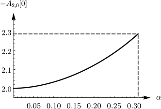
Figure 1: Absolute value of $A_{2,0}[0]$ (calculated by means of Padé approximants) as a function of $\alpha$. The dashed lines indicates the position of $\alpha_{c}^{(2,0)}$ and the corresponding value of the coefficient $A_{2,0}[0]$.

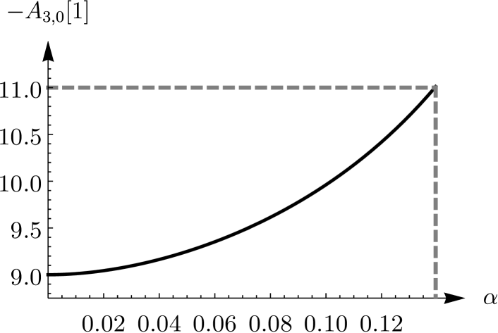
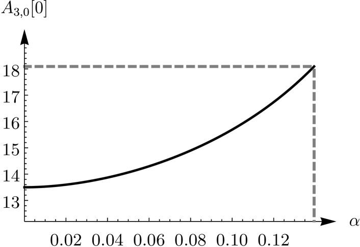
Figure 2: Absolute value of $A_{3,0}[1]$ and $A_{3,0}[0]$ (both calculated by means of Padé approximants) as a function of $\alpha$. The dashed lines indicates the position of $\alpha_{c}^{(3,0)}$ and the corresponding value of the coefficient $-A_{3,0}[1]$ and $A_{3,0}[0]$.

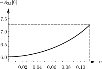
Figure 3: Absolute value of $A_{3,1}[0]$ (calculated by means of Padé approximants) as a function of $\alpha$. The dashed lines indicates the position of $\alpha_{c}^{(3,1)}$ and the corresponding value of the coefficient $A_{2,0}[0]$.

III.5 Variational Calculation and its Accuracy

We carried out variational calculations for the states with quantum numbers $(1,0)$, $(2,0)$ and $(2,1)$. A computational code was written in FORTRAN 90 in other to perform variational calculations. The integration routine was designed using the algorithm described in Integracion . The optimization of the variational parameters was performed by means of the MINUIT routine Minuit of CERN-LIB.

In Table 7 we present variational energies of the states (1,0) and (2,1) for different values of $\alpha$. We also present their corresponding corrections and approximations (49) up to third order in PT. In Table 8 we present the variational energy of the state (2,0). For this state we include up to the second order corrections and the corresponding approximations of the energy. Additionally, Table 8 contains the zeroth and first order approximation of the position of the radial node.

We must emphasize that the nodal surface of the exact wave functions of the states $(1,0)$ and ($2,1$) do not depend on $\alpha$. Of course this information is codified in their corresponding trial functions $\Psi_{1,0}^{(t)}$ and $\Psi_{2,0}^{(t)}$, see (41). Therefore, no correction to the nodal surface has to be calculated. In contrast, the state (2,1) develops a node at finite $r\neq 0$ which can be only approximated by numerical means. For this state, following (41), the trial function reads

$$\Psi_{2,0}^{(t)}(r)\ =\ \left(r-r_{0}^{(0)}\right)\,e^{-\Phi_{2,0}^{(t)}}\,,$$ (60)

where $r_{0}^{(0)}$ is the zeroth order approximation of the position of the node. In fact $r_{0}^{(0)}$ is determined from the orthogonality constraint that we impose between the trial functions of the states (1,0) and (2,0),

$$r_{0}^{(0)}\ =\ \frac{\int_{0}^{\infty}e^{\Phi_{1,0}^{(t)}}\,e^{-\Phi_{2,0}^{(t)}}\,r^{3}\,dr}{\int_{0}^{\infty}e^{\Phi_{1,0}^{(t)}}\,e^{-\Phi_{2,0}^{(t)}}\,r^{2}\,dr}\ .$$ (61)

The first order correction of $r_{0}^{(0)}$ must be a constant and, from equation (LABEL:eq:kcorrection) together with boundary conditions (14), one can show that it is given by

$$r_{0}^{(1)}\ =\ \frac{2\int_{0}^{r_{0}^{(0)}}(E_{2,0;1}-V^{(1)})\,\left(\Psi_{2,0}^{(t)}\right)^{2}\,r^{2}\,dr}{\left(r_{0}^{(0)}\right)^{2}\,e^{-2\Phi_{2,0}^{(t)}}}\ .$$ (62)

Higher order corrections $r_{0}^{(k)}$ with $k>1$ can be calculated, however, the higher order correction, the more cumbersome calculations have to be performed. As one can expect, the calculation of the corrections in PT is simpler if the exact function $f_{n,l}(r)$ is known.

Table 7: Variational energy of the state $(1,0)$ and $(2,1)$ for some selected values of $\alpha$. We present up to the third order correction in PT. For corrections and approximations of different order we take the notation used in (49). The digits presented for $E_{1,0;3}$ correspond to digits verified with Padé approximants and the Lag-Mesh.

$\alpha$	-$E_{1,0;1}$	$E_{1,0}^{(2)}$	-$E_{1,0;2}$	$\quad\quad E_{1,0}^{(3)}$	-$E_{1,0;3}$
0.01	$0.4900745066986851$	-$4.80011\times 10^{-11}$	$0.4900745067466863$	-$7.97\times 10^{-15}$	$0.4900745067466942$
0.10	$0.40705803060984105$	-$3.56285\times 10^{-12}$	$0.40705803061340390$	$7.58\times 10^{-16}$	0.40705803061340315
0.50	$0.148117017843659$	-$4.046202\times 10^{-9}$	$0.148117021889861$	-$7.13\times 10^{-14}$	$0.148117021889933$
1.00	$0.01028575123218$	-$3.874918\times 10^{-8}$	$0.01028578998128$	-$8.7607\times 10^{-12}$	$0.01028578999004$
$\alpha$	-$E_{2,1;1}$	$E_{2,1}^{(2)}$	-$E_{2,1;2}$	$E_{2,1}^{(3)}$	-$E_{2,1;3}$
0.01	0.115245224090557422	-$6.762\times 10^{-15}$	0.115245224090564185	-$3.7\times 10^{-20}$	0.115245224090564185
0.10	0.046534388129	-$2.341\times 10^{-9}$	0.046534390471	-$1.52\times 10^{-11}$	0.046534390486
0.15	0.021104690	-$1.924\times 10^{-7}$	0.021104882	-$5.80\times 10^{-9}$	0.021104888
0.20	0.004093	-$6.84\times 10^{-6}$	0.004100	-$7.16\times 10^{-7}$	0.004101

Table 8: Variational energy of the first state (2,0) and its corrections in PT for some selected values of $\alpha$. For corrections and approximations of different order we take the notation used in (49). The digits presented for $E_{1,0;2}$ and $r_{0}^{(0)}+r_{0}^{(1)}$ correspond to digits verified with Padé approximants and the Lag-Mesh.

$\alpha$	-$E_{2,0;1}$	$\quad\quad E_{2,0}^{(2)}$	-$E_{2,0;2}$	$\quad\quad r_{0}^{(0)}$	$\quad\quad r_{0}^{(1)}$	$r_{0}^{(0)}+r_{0}^{(1)}$
0.01	0.11529328517404	$6.05\times 10^{-12}\quad$	0.11529328516799	2.000381392	-$8.519\times 10^{-6}\quad$	2.000389912
0.10	0.0499282672	-$4.05\times 10^{-9}$	0.0499282713	2.03333727	$5.2755\times 10^{-5}$	2.03328451
0.2	0.012104	-$3.27\times 10^{-6}$	0.012107	2.12385	0.00120	2.12266
0.25	0.00336	-$2.48\times 10^{-5}$	0.00339	2.189	0.0008	2.188

Results indicates that PT developed for the variational energy leads to a fast convergent series. Therefore, equation (50) should be fulfilled. In the case of the ground state (1,0) we are able to provide 14 - 17 exact digits in the range $0\leq\alpha\leq 1$. For the three states studied, the variational calculation of energy becomes less accuracy as $\alpha\rightarrow\alpha_{c}$. In general, the trail function with optimized parameters becomes very flat. In this regime, by calculating corrections of the energy we obtain a slow convergent series. For the state (2,0) we obtain also a high accurate value for the position of the node which agree with previous results presented in Table 6.

The Non-Linearization Procedure allows us to estimate the absolute deviation between the exact wave function $\Psi_{n,l}$ and the trial function $\Psi_{n,l}^{(t)}$. For example, for the ground state we obtain a very small deviation

$$|\Psi_{1,0}(r)-\Psi_{1,0}^{(t)}(r)|<1\times 10^{-4}\ ,$$ (63)

in the domain $0\leq r<\infty$ with $0\leq\alpha<1$. In this sense, we conclude that the trial wave function $\Psi_{1,0}^{(t)}$ that we designed is locally accurate. For the states (2,0) and (2,1) the same situation occurs.

III.6 Analytic Expression for $E_{n,l}$

Following the prescription described in interpolaciones we construct analytical expressions of the energy $E_{n,l}$. We use the expansion of the energy in the regime of PT (11) and the expansion in the neighborhood of the critical parameter (5,6) in order to construct a compact interpolating function.

The interpolating function is a rational function with free parameters to be adjusted by least squares. The expansions of the interpolating functions at $\alpha\rightarrow 0$ and $\alpha\rightarrow\alpha_{c}^{(n,l)}$ must reproduce functionally the expansions (11), (5,6). In order to do this, four restrictions are introduced such that only the dominant and subdominant terms of each expansion are exactly reproduced.

For the states with angular momentum $l=0$ we propose the function

$$E_{n,0}(\alpha)=\frac{\sum_{i=2}^{M}c_{i}^{(n,0)}(\alpha_{c}^{(n,0)}-\alpha)^{i}}{\sum_{j=0}^{N}d_{j}^{(n,0)}(\alpha_{c}^{(n,0)}-\alpha)^{j}}\,,$$ (64)

where $c_{i}^{(n,0)}$ and $d_{j}^{(n,0)}$ are parameters. The parameter $d_{0}^{(n,0)}$ is fixed to the unity as a normalization. In this case the function contains $M+N-5$ free parameters. For states with $l\neq 0$ we propose the function

$$E_{n,l}(\alpha)=\frac{\sum_{i=2}^{M}c_{i}^{(n,l)}(\alpha_{c}^{(n,l)}-\alpha)^{i/2}}{\sum_{j=0}^{N}d_{j}^{(n,l)}(\alpha_{c}^{(n,l)}-\alpha)^{j}}\,,$$ (65)

where $c_{i}^{(n,l)}$ and $d_{j}^{(n,l)}$ are parameters and $d_{0}^{(n,l)}$ is fixed to the unity. In this case the interpolating function also contains $M+N-5$ free parameters.

For all cases, $M=N=4$ is the the minimal value which provides at least $6$ correct digits for any value of $\alpha$. In Table 9 we present the fitted parameters of the states (1,0), (2,0) and (2,1).

Table 9: Fitted parameters of the interpolating functions (64) and (65) for some states $(n,l)$.

$(n,l)$	$c_{2}^{(n,l)}$	$c_{3}^{(n,l)}$	$c_{4}^{(n,l)}$	$d_{1}^{(n,l)}$	$d_{2}^{(n,l)}$	$d_{3}^{(n,l)}$	$d_{4}^{(n,l)}$
(1,0)	-0.274683	0.273223	-0.064690	-1.147158	0.369868	-0.0228517	-0.001716
(2,0)	-0.867186	0.297361	2.965554	-1.658874	-1.40866	0.481608	1.367597
(2,1)	-0.126016	-0.418180	-0.840617	-0.0330058	-3.268627	9.004197	-15.528311

IV Conclusions

The Yukawa potential is studied using three different approaches: PT, Lag-Mesh and VM. Perturbation series in powers of $\alpha$ are calculated algebraically within the framework of the Non-Linerazation Procedure. It is shown that the Padé approximants related to the PT series of the energy provide 13 - 14 exact decimal digits which are in agreement with the Lag-Mesh calculations. The methods of PT (+ Padé approximants) and Lag-Mesh describe correctly the behavior of a particle in the Yukawa potential even near the critical parameters where the states become weakly bound. For all states considered, we reproduce or even exceed the precision of the critical screening parameters that are known in the literature to the authors at the moment. The nodes of the radial wave function are found for various states and also exhibit a good agreement between the three methods. The Padé approximants allow us to calculate the nodes as the roots of some polynomials. We design a locally accurate and compact trial function whose absolute deviation from the exact wave function is less than $10^{-4}$ in the range of $r$. Together with perturbative corrections within the Non-Linearization Procedure, the trial function leads to highly accurate estimates of the energy comparable with other numerical methods (in particular, Lag-Mesh). The knowledge of a highly accurate trial functions will allow to calculate transition amplitudes with high accuracy and hence to create a theory of radiative transitions for the Yukawa potential. Finally, a remarkable analytical expression for the energy of several states is obtained: it reproduces 6 significant digits correctly in the entire physical range of the screening parameter $\alpha$.

References

- (1) H. Yukawa, On the interaction of elementary participles, Proc. Phys. Math. Soc. Jap 17, 48 (1935).
- (2) C. Henning et al., Ground state of a confined Yukawa plasma, Phys. Rev. E, 74, 056403 (2006).
- (3) H. Khälert and M. Bonitz, Fluid modes of a spherically Yukawa Plasma, Phys. Rev. E, 82, 036407 (2010).
- (4) H. Totsuji, T. Kishimoto, C. Totsuji, T. Sasabe, Structure of Yukawa dusty plasma mixtures, Phys. Rev. E, 58, 7831 (1998).
- (5) A. Loeb and N. Weiner, Cores in Dwarf Galaxies from Dark Matter with a Yukawa Potential, Phys. Rev. Lett. 106, 171302 (2011).
- (6) Y. Z. Lin, Y. G. Li, J. D. Li, Study on multi-Yukawa potential between charged colloid particles, J. Mol. Liq. 125, 29-36 (2006).
- (7) A. K. Roy, Critical parameters and spherical confinement of H in screened Coulomb potential, Int. J. Quantum Chem. 116, (2016).
- (8) C. S. Lam and Y. P. Varshni, Energies of eigenstates in a static screened coulomb potential Phys. Rev. A 4, 1875 (1971).
- (9) C. Stubbins, Bound states of the Hulthen and Yukawa potentials , Phys. Rev. A 48, 220 (1993).
- (10) O. A. Gomes, H. Chacham and J. R. Mohallem, Variational calculations for the bound-unbound transition of the Yukawa potential, Phys. Rev. A, 50, 228-231 (1994).
- (11) V. M. Vainberg, V. L. Eletskii, V. S. Popov, Logarithmic perturbation theory for screened Coulomb potential and a charmonium potential, Sh. Eksp. Ther Fiz, 81, 1567-1582 (1981).
- (12) P. Serra, J. P. Neirotti, S. Kais, Finite scaling in quantum mechanics, J. Phys. Chem. A, 102, 9518-9522 (1998).
- (13) C. G. Diaz, F. M. Fernández and E. A. Castro, Critical screening parameters for screened Coulomb potentials, J. Phys. A, 24, 2061-2068 (1991).
- (14) J. Rogers, H. C. Graboske and D. J. Harwood, Bound eigenstates of the static screened Coulomb potential Phys. Rev. A 1, 1577 (1970).
- (15) J. P. Edwards et al., The Yukawa potential: ground state energy and critical screening, Progr. Theor. Exp. Phys. 8 (2017).
- (16) H. E. Montgomery, K. D. Sen and J. Katriel, Critical screening in the one- and two-electron Yukawa atoms, Phys. Rev. A 97, 022503 (2018).
- (17) M. Klaus and B. Simon, Coupling constants thresholds in non relativistic quantum mechanics. I. Short-range two body case, Ann. Phys. 130, 2 (1980).
- (18) A. V. Turbiner, The eigenvalue spectrum in quantum mechanics and the nonlinearization procedure, Phys. Usp. 27, 668-694 (1984).
- (19) E. Vrscay, Hydrogen atom with Yukawa potential: Perturbation theory and continued-fractions-Padé approximants at large order, Phys. Rev. A, 33, 1433-1436 (1986).
- (20) D. Baye, The Lagrange-mesh method, Phys. Rep. 565, 1 (2015).
- (21) D. Bressanini, P. J. Reynolds, Generalized variational principle for excited states using nodes of trial functions, Phys. Rev. E, 84 (2011).
- (22) P. J. Reynolds, D. M. Ceperley, B. J. Alder and W. A. Lester Jr., Fixed‐node quantum Monte Carlo for molecules a) b), J. Chem. Phys 77, 5593-5603 (1983).
- (23) A. V. Turbiner, The hydrogen atom in an external magnetic field, J. Phys. A: Math. Gen. 17, 859 (1984).
- (24) C. S. Lai, Padé approximants and perturbation theory for screened Coulomb potentials, Phys. Rev. A 23, 455 (1981).
- (25) D. Baye, L. Filippin, M. Godefroid, Accurate solution of the Dirac equation on Lagrange meshes, Phys. Rev. E 89, 043305 (2014) .
- (26) D. Baye, Integrals of Lagrange functions and sum rules, J. Phys. A 44 (2011) 395204.
- (27) V. Szalay, Discrete variable representations of differential operators, J. Chem. Phys. 99, 1978 (1993).
- (28) A. V. Turbiner, Anharmonic oscillator and double-well potential: approximating eigenfunctions, Lett. Math. Phys. 74, 169-180 (2005).
- (29) E. Anderson, et al., LAPACK User’s Guide, SIAM, (1992).
- (30) A. Genz and A. Malik, An adaptive algorithm for numerical integration over an N-dimensional rectangular region, J. Comput. Appl. Math. 6(4), 295–302 (1980).
- (31) F. James and M. Roos, Minuit-a system for function minimization and analysis of the parameter errors and correlations, Comput. Phys. Commun. 10, 343–367 (1975).
- (32) A. V. Turbiner, J. C. López-Vieyra, H. Olivares Pilón, J. C. del Valle, and D. J. Nader, Ground state energy in quantum mechanics: Interpolating between weak and strong coupling regime (work in progress).