Characteristic interfacial structure behind a rapidly moving contact line

Abstract

In forced wetting, a rapidly moving surface drags with it a thin layer of trailing fluid as it is plunged into a second fluid bath. Using high-speed interferometry, we find characteristic structure in the thickness of this layer with multiple thin flat triangular structures separated by much thicker regions. These features, depending on liquid viscosity and penetration velocity, are robust and occur in both wetting and de-wetting geometries. Their presence clearly shows the importance of motion in the transverse direction. We present a model using the assumption that the velocity profile is robust to thickness fluctuations that gives a good estimate of the thin gap thickness.

Introduction: A solid entrains surrounding air along with its moving surface when it is pushed rapidly into a liquid bath. In this process, known as “forced wetting”, a three-phase contact line between the substrate, air and liquid is forced to move across the surface of the solid. If the penetration velocity is high enough, the contact-line distorts downwards to create a pocket of air. The effects of such entrainment are observed in the form of entrapped bubbles that can be problematic in printing and coating technologies.

When the substrate velocity, $U$, is low, the contact line remains approximately level with the liquid surface. At higher velocity, the line distorts and evolves towards a steady-state “V” shape Perry (1967); Burley and Kennedy (1976); Blake and Ruschak (1979) shown schematically in Fig. 1a. The top row of Fig. 1b shows images, spaced $100ms$ apart, of the transient evolution to this shape. The first frame shows the contact line immediately after a plastic substrate starts to move at fixed velocity into a liquid bath; the next images show the development towards the steady-state “V” shown in the last frame.

These images, taken with white light, show the lateral evolution of the contact line but provide no information about the thickness of the air gap at different points across its surface. We obtain such information from interference fringes, which are visible when the optical path across the gap is less than the coherence length of the light. In the bottom panel of Fig. 1b, interference fringes appear for thicknesses less than $\approx 30\mu m$. These images reveal unexpected structure in the gap thickness that was not visible in the top panel.

As the contact line evolves, the air gap is thick near the edge and becomes thin and extremely flat in the center. This flatness can be ascertained because over regions of approximately $5mm$ in width there are only two fringes. These correspond to equal-height contours, with a difference in thickness between successive bright fringes of $\approx 0.32\mu m$. Once the contact line has formed the “V” shape, the air gap continues to evolve until it reaches a steady shape shown in the last frame; at that point the air pocket has two very flat triangular structures that are symmetrically placed in the upper corners of the gap separated by an intervening thicker region.

These features are very robust. They appear regardless of the solid material (e.g., metal or plastic) and the fluid viscosity; they appear if the air is replaced by a second liquid. More surprisingly, similar structures appear in de-wetting experiments where the liquid drains from the substrate as it is withdrawn from the bath.

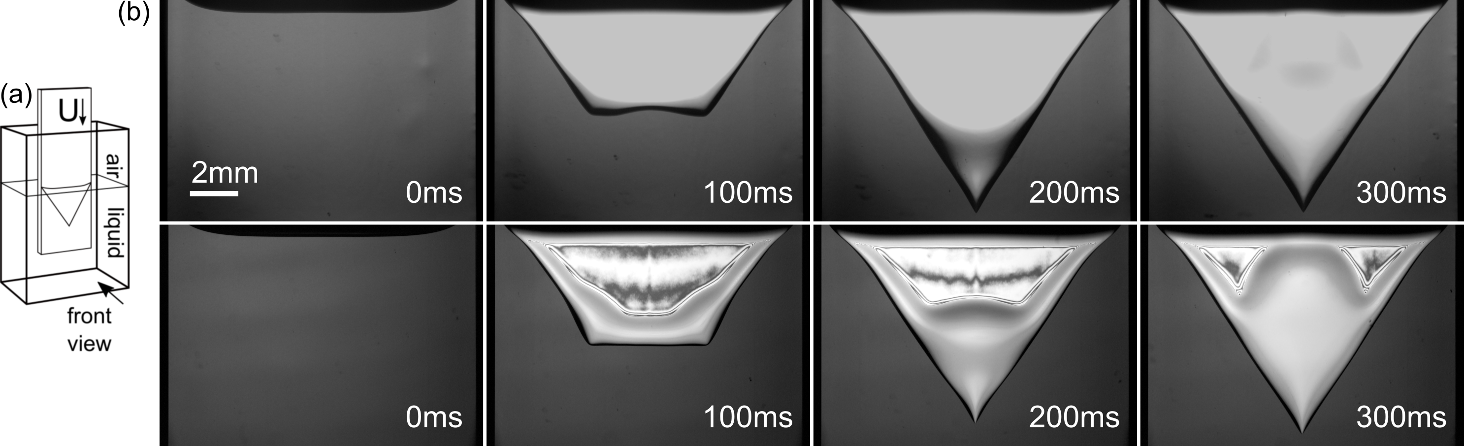
Figure 1: (a) Schematic showing the “V”-shaped steady-state contact line as viewed from the front. (b) Images during the evolution of the “V” shape spaced $100ms$ apart. A $12.7mm$ wide tape travels vertically into a water/glycerol mixture of viscosity, $\eta=226cP$, at $U=130mm/s$. Top row: Images using a white light. Bottom row: Images using red light of coherence length $60\mu m$. Interference patterns appear where the air pocket is thinner than $60\mu m/2=30\mu m$.

We measured the dependence of the gap dimensions on the liquid viscosity, substrate width, and penetration velocity. The absolute thickness at different points in the gap were measured in order to characterize the three-dimensional structure of the air pocket.

Methods: In our experiments, we used flexible Mylar tape as the solid substrate. The tape was held vertically as it was forced into (wetting) or pulled out of (de-wetting) the bath. Vibrations and twist were minimized by supports located along the path of the tape. These and the chamber walls were kept distant from the air pocket to avoid any interactions Vandre et al. (2012, 2014). Except where specifically stated otherwise, the tape width was $12.7mm$. In each run, the tape velocity, $U$, was held constant at speeds between $50mm/s$ and $1000mm/s$.

The liquid bath consisted of water/glycerol mixtures whose viscosity, $\eta_{out}$, could be tuned between different runs by varying the relative concentration of the components: $26cP\leq\eta_{out}\leq 572cP$. In order to check whether the structure of the gap was robust to the type of entrained fluid, we also replaced the air by a silicon oil of viscosity $0.65cP$. Interfacial tensions, $\gamma$, and densities, $\rho$, were measured for different mixtures to be between $53mN/m$ and $66mN/m$ and between $1.21g/cm^{3}$ and $1.25g/cm^{3}$ respectively.

The absolute thickness, $H(x,y)$, of the air gap at different points on the surface $(x,y)$, was measured using high-speed interferometric imaging Driscoll and Nagel (2011) from multiple wavelengths of light simultaneously Tran et al. (2012); van der Veen et al. (2012); Bouwhuis et al. (2012). Once the thickness of the thin regions is known, the thickness of the gap in the thicker regions can be measured by counting fringes from a laser (see Supplemental Information).

Role of viscosity and evolution to steady state: The “V” shape of the steady-state contact line was quantitatively interpreted by Blake and Ruschak Blake and Ruschak (1979) in terms of a maximum contact-line velocity $U_{max}$ with which the liquid can wet the solid. When $U>U_{max}$, the contact line is forced to tilt by an angle $\phi$ so that the normal velocity of the contact line does not surpass this threshold:

$$Ucos\phi=U_{max}.$$ (1)

In the Supplemental information we compare $U_{max}$ to the normal relative velocity at each point of the contact-line filmed during its evolution from an initial horizontal line into the final “V” shape.

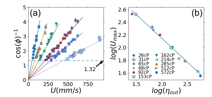
Figure 2: (a) $(cos\phi)^{-1}$ versus velocity $U$ for water/glycerol mixtures with viscosities between $26cP$ and $572cP$. Solid lines: least-square-fits to Eq. 1. (b) $U_{max}$ extracted from (a), versus $\eta_{out}$. Solid line: $U_{max}\sim\eta_{out}^{-0.75}$.

Figure 2a shows $(cos\phi)^{-1}$ versus $U$ for liquids of different viscosities, $\eta_{out}$. (Due to growing fluctuations in the contact line as $U$ decreases towards $U_{max}$, our data does not extend below $(cos\phi)^{-1}\approx 1.3$.) Figure 2b shows that $U_{max}$ determined from Eq. 1 varies as

$$U_{max}\sim\eta_{out}^{-0.75\pm 0.03}.$$ (2)

This exponent is similar to that found in earlier works Perry (1967); Wilkinson (1975); Burley and Kennedy (1976); Gutoff and Kendrick (1982); Burley and Jolly (1984); Buonopane et al. (1986); Blake and Ruschak (1997) but is larger than the value (between $1/3$ and $1/2$) suggested by Marchant et al. Marchand et al. (2012).

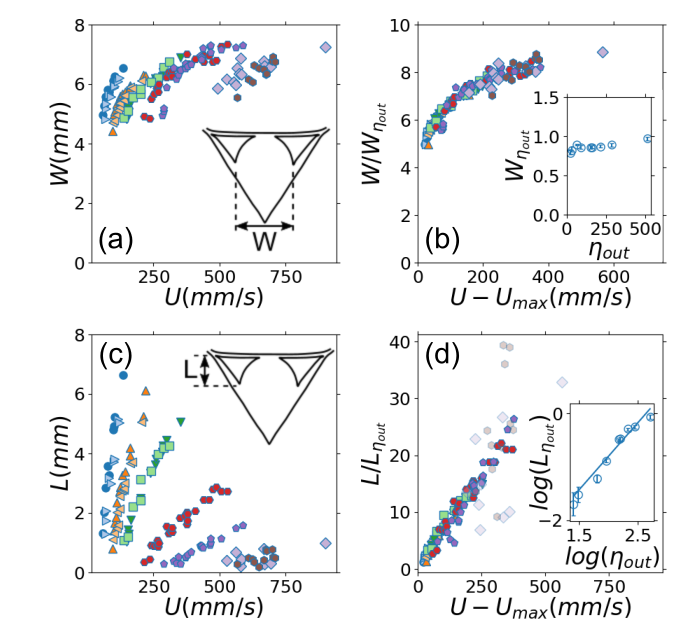
Figure 3: Lateral geometry of thin structures in the air gap. (a) Distance between tips, $W$, versus $U$. (b) Data collapse of the form $W/W_{\eta_{out}}=F_{W}(U-U_{max})$. Inset: $W_{\eta_{out}}$ versus $\eta_{out}$. (c) Vertical span $L$ versus $U$. (d) Data collapse of the form $L/L_{\eta_{out}}=F_{L}(U-U_{max})$. Inset: $L_{\eta_{out}}$ versus $\eta_{out}$. Line $L_{\eta_{out}}\propto\eta_{out}^{1.3}$.

Structure within the steady-state air gap: As the images in the bottom row of Fig. 1(b) make clear, there is considerable structure in the thickness of the air gap, $H(x,y)$. Most striking is the unexpected appearance of two flat steady-state triangular shapes in the upper corners of the last image.

Figure 3a shows $W$, the tip separation of the triangular regions indicated in the inset, versus $U$. Figure 3b shows that the data can be collapsed to a form: $W/W_{\eta_{out}}=F_{W}(U-U_{max})$. The inset shows the empirical fitting parameter $W_{\eta_{out}}\approx 1$ for all $\eta_{out}$. $W$ appears to saturate at large $U$. Figure 3c shows $L$, the vertical span of the triangular regions, versus $U$. The slope of $L$ versus $U$ increases with increasing bath viscosity. In Fig. 3d we collapsed the data using the form: $L/L_{\eta_{out}}=F_{L}(U-U_{max})$ where $L_{\eta_{out}}$ is an empirical fitting parameter shown in the inset. With the exception of low $\eta_{out}$ where there are large fluctuations (shown as translucent), the collapse is good with $L_{\eta_{out}}\propto\eta_{out}^{1.3\pm 0.1}$.

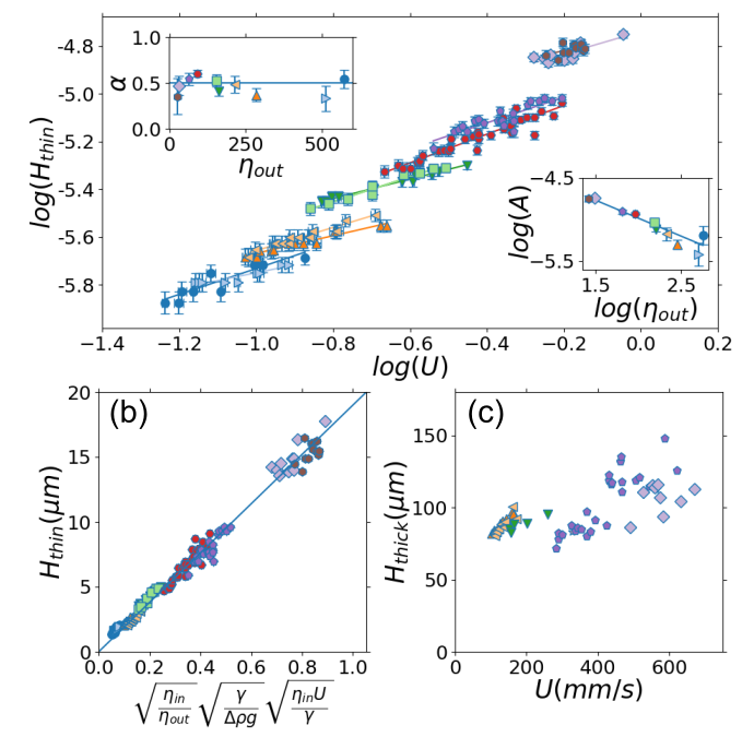
Figure 4: Thickness of air gap. (a) Thickness of the thin triangular regions measured at their centers, $H_{thin}$, versus $U$. Lines show fits for $H_{thin}\propto A*U^{\alpha}$. Upper inset: $\alpha$ versus $\eta_{out}$. The average $<\alpha>\approx 0.46\pm 0.03$. Lower inset: $A$ versus $\eta_{out}$. Line shows fit $A\propto\eta_{out}^{-0.43}$. (b) Data collapsed to Eq. 8. (c) Thickness at thickest point of the gap, $H_{thick}$, versus $U$.

An average thickness of the air gap was previously estimated to be between $0.05\mu m$ and $0.9\mu m$ (e.g., see  Perry (1967); Miyamoto (1991)); in the case of a plunging liquid jet (instead of plunging solid) it was measured to be several microns Lorenceau et al. (2004). No structure within the gap was reported.

In Fig. 4(a) we show $H_{thin}$, the absolute thickness of the gap in the center of the triangular regions obtained from the multi-wavelength interference method described in Supplemental Information, versus $U$. These regions are extremely flat with a height variation of only $\Delta H_{thin}\approx 0.1\sim 0.7\mu m$ depending on the outer fluid viscosity. As one might naively expect, $H_{thin}$ increases with increasing penetration velocity. Each data set starts only when $U>U_{max}$ (from Fig. 2(b)); thus as $\eta_{out}$ increases, the data range shifts to lower velocities.

The data for different values of $\eta_{out}$ do not fall on top of one another but splay out and are roughly parallel to one another. We fit each data set to the form: $H_{thin}=A*U^{\alpha}$. The insets in Fig. 4a show the least-square-fits of the parameters $\alpha$ and $A$ versus $\eta_{out}$. The upper inset shows that the average $\alpha=0.46\pm 0.03$. The lower inset shows $A\propto\eta_{out}^{\beta}$ with a best-fit exponent $\beta=-0.43\pm 0.07$ (solid line). This suggests the form:

$$H_{thin}\propto\sqrt{\frac{\gamma}{\Delta\rho g}}\bigg{(}\frac{\eta_{in}U}{\gamma}\bigg{)}^{0.46\pm 0.03}\bigg{(}\frac{\eta_{in}}{\eta_{out}}\bigg{)}^{0.43\pm 0.07}$$ (3)

where$\Delta\rho g$ is the buoyancy force and $\eta_{in}$ is the inner fluid viscosity (air in this case).

In order to understand this behavior, we model the air flow within the gap. Because the contact line is stationary in the lab frame, the total flux of air must be zero; any air that is entrained by the substrate must have a return path to the surface. (This is different from the situation of depositing a liquid layer on an infinite substrate pulled out of a bath Landau and Levich (1942); Derjaguin (1943)). The case where there is no lateral flow so that the geometry is a two-dimensional wedge with fluid-substrate contact angle $\theta$ is treated by Huh & Scriven Huh and Scriven (1971). However, in the situation of forced wetting, with the “V” shape, there is clearly transverse flow. The central, thickest part of the gap can accommodate the return of most of the entrained air so that in the very thin triangular regions there need not be any return flow. In those thin regions, the entrained air can escape by flowing downwards towards the contact line and then sideways towards the central thicker part of the gap. Our experiments show a different flow field than the scheme proposed by Severtson & Aidun Severtson and Aidun (1996).

We assume that the overall velocity of the liquid/liquid interface, $U_{I}$, is still given by the two-dimensional results of Huh & Scriven:

$$U_{I}=\zeta U\approx(1-D_{\theta}\frac{\eta_{in}}{\eta_{out}})U$$ (4)

where $D_{\theta}$ depends on contact angle $\theta$ and the second approximate expression is valid near $\theta\approx 2^{\circ}$ over the experimental range of $\eta_{in}/\eta_{out}$. We assume that $U_{I}$ is determined by the average air flow in the gap, which is dominated by the thicker regions, and does not vary significantly across the surface.

In the thin regions, where the liquid interface is nearly vertical, the buoyancy force is balanced by the viscous forces in the inner fluid: $\eta_{in}\partial^{2}u(y)/\partial y^{2}=\Delta\rho g$ where $y$ is in the horizontal direction perpendicular to the substrate surface and the flow is in the $z$ direction. Using the boundary conditions at the substrate $u(y=0)=U$ and at the liquid/liquid interface $u(y=H_{thin})=U_{I}$ we find:

$$u=\frac{\Delta\rho g}{2\eta_{in}}y^{2}+By+U$$ (5)

$$\text{with }B=-\bigg{(}\frac{(1-\zeta)U}{H_{thin}}+\frac{\Delta\rho g}{2\eta_{in}}H_{thin}\bigg{)}.$$ (6)

Given an arbitrary $H_{thin}$ there is a solution satisfying both boundary conditions. In order to determine which solution is chosen, we argue that the system selects the one that is invariant to thickness fluctuations. Any noise or vibration in the flow can perturb $H_{thin}$ and disrupt the flows. If the velocity profile is invariant to such fluctuations it will be stationary and robust against such noise with the least “wandering” of the system in the flow-field phase space. Thus the system chooses the solution where $B$ is an extremum. In that case, not only is $B$ independent of $H_{thin}$, but the profile has zero slope at the liquid/liquid interface. Setting $dB/dH_{thin}=0$ gives:

$$H_{thin}=\sqrt{2(1-\zeta)}\sqrt{\frac{\gamma}{\Delta\rho g}}\sqrt{\frac{\eta_{in}U}{\gamma}}$$ (7)

(We note that this is the same solution as would be obtained by assuming minimum dissipation.)

Inserting Eq. 4 for $\zeta$ leads to:

$$H_{thin}=D_{\theta}\sqrt{\frac{\eta_{in}}{\eta_{out}}}\sqrt{\frac{\gamma}{\Delta\rho g}}\sqrt{\frac{\eta_{in}U}{\gamma}}.$$ (8)

Comparing Eq. 8 to our data in Fig. 4b shows an excellent agreement with $D_{\theta}\approx 19$ corresponding to $\theta=2.7^{\circ}$.

To see if $\theta=2.7^{\circ}$ is reasonable for our experiment, we measure $H_{thick}$, the thickness of the air pocket at its maximum height (near the center of the “V” shape). Figure 4c shows that $H_{thick}$ is typically $\sim 100\mu m$, which is more than an order of magnitude larger than $H_{thin}$, and has large fluctuations. From $H_{thick}$ and the dimensions of the “V” shape, we estimate $\theta$ to be between $1^{\circ}$ and $4^{\circ}$. Thus, this model for the air flow in the thin regions is in quantitative agreement with our data. When the substrate width is varied, the number of thin regions in the air gap varies but leaves the distance, $W$, between them roughly constant. Figure 5a shows an image of such an entrained layer for a $25.4mm$ wide tape (i.e., twice as wide as was used in the data shown above) with more thin-thick alternations across the tape surface. Similar thin triangles appear if the air is replaced by another fluid as shown in Fig. 5b where a $12.7mm$ tape moves between a $0.65cP$ silicone oil and a $60cP$ water/glycerol mixture. Two thin triangular regions appear in the upper corners of the “V”. If we reverse the direction of $U$, so that the solid emerges from the bath and the liquid de-wets the substrate, a liquid film forms with three thin regions (now near the bottom) as shown in Fig. 5c. Rim-like structure behind the contact line in the longitudinal direction was previously seen in de-wetting Redon et al. (1991); Snoeijer et al. (2006, 2008); Maleki et al. (2011), but no transverse thickness modulation was reported. As with forced wetting, increasing the substrate width produces more thin-thick alternations while leaving the distance $W$ between thin parts roughly constant. Thus these thin triangular regions are a robust feature under both wetting and de-wetting conditions.

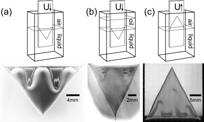
Figure 5: Robustness of structure for wetting and de-wetting geometries as shown in schematics. (a) A wide $25.4mm$ tape moving from air into an $150cP$ water/glycerol bath showing four thin regions. (b) A $0.65cP$ silicone oil (replacing air) above a $60cP$ water/glycerol mixture. A tape of width $12.7mm$ was used showing two thin triangular regions. (c) A tape of width $25.4mm$ pulled out of a water bath into air showing three thin regions. Gray scale inverted for clarity in (a) and (b).

Summary: We have found an unexpected characteristic entrained layer in forced-wetting and de-wetting experiments. This generic structure, consisting of extremely flat thin sections alternating with thick pockets, is stable and is controlled by viscosity contrast between the inner and outer fluids, the penetration velocity and width of the substrate.

Forced wetting is very different from wetting caused by a drop impacting a solid and spreading radially. In that case, the contact line does not slide smoothly across the substrate; rather it moves by the nucleation of touch-down events near the encroaching interface. The air gap breaks down at spots where the liquid film above it makes local contact with the surface Driscoll and Nagel (2011); Driscoll et al. (2010); Thoroddsen et al. (2010); Kolinski et al. (2012). Our forced-wetting experiments show no such re-wetting holes.

For thin film problems such as gravitational flows, liquid films in rotating cylinders (i.e., the printer’s instability), spinning drops and circular hydraulic jumps, the instability along the direction perpendicular to the general motion of the fluid has been observed and analyzed Huppert (1982); Troian et al. (1989); Thoroddsen and Mahadevan (1997); Rabaud et al. (1991); Hosoi and Mahadevan (1999); Melo et al. (1989); Bush et al. (2006). On the other hand, many attempts to understand wetting ignore motion transverse to the velocity of the substrate Oron et al. (1997). Such a simplification reduces the problem to a two-dimensional geometry. While effective in describing the onset of the forced-wetting transition Snoeijer et al. (2007); Delon et al. (2008); Eggers (2004); Snoeijer et al. (2006, 2008); Vandre et al. (2013); Sprittles (2017), such analyses exclude the three-dimensional structures that emerge at later stages. Our experiments show a pure two-dimensional analysis is no longer adequate in the steady state. A uniform longitudinal velocity profile is unstable to transverse modulation; air in the thin regions of the gap flows in the direction of substrate motion and only in the thicker regions is there a return flow to the surface of the entrained air. Our argument that assumes the velocity profile is robust to thickness fluctuations gives an excellent estimate for the flow profile in the thin regions.