Embeddings for the space $LD_{\gamma}^{p}$ on sets of finite perimeter

Abstract.

Given an open set with finite perimeter $\Omega\subset\mathbb{R}^{n}$, we consider the space $LD_{\gamma}^{p}(\Omega)$, $1\leq p<\infty$, of functions with $p$th-integrable deformation tensor on $\Omega$ and with $p$th-integrable trace value on the essential boundary of $\Omega$. We establish the continuous embedding $LD_{\gamma}^{p}(\Omega)\subset L^{pN/(N-1)}(\Omega)$. The space $LD_{\gamma}^{p}(\Omega)$ and this embedding arise naturally in studying the motion of rigid bodies in a viscous, incompressible fluid.

1. Introduction

In this work, we establish Sobolev-type embeddings for a non-standard function space that arise in the study of the motion of rigid bodies in a viscous, incompressible fluid.

The problem of the motion of solid bodies in a viscous fluid filling a bounded container, has been studied by several authors — we cite, in particular, Hoffmann, Starovoitov [21], San Martín, Starovoitov, Tucsnak [30], Feireisl, Hillairet, Nečasová [13], Bost, Cottet, Maitre [8], Gunzburger, Lee, Seregin [16], Takahashi [32], Judakov [39]. The authors of these works considered the no-slip condition, that is, the velocity is assumed to equal the velocity at the surface of the rigid bodies and the velocity of the container walls, also assumed rigid. In the simplest case in which the container is fixed, the velocity vanishes at the walls.

However, it has been shown mathematically that this assumption leads to some non-physical results, namely, under the no-slip condition collision between the bodies and between the bodies and the walls cannot happen in finite time (see Hesla [19], Hillairet [20], Starovoitov [31] among others).

One way to include the possibility of collision that is physically motivated is to allow slippage at the boundaries. There are several ways to allow for a non-trivial slip at the boundary by modifying the boundary condition. The Navier boundary condition models slip with friction and it is amenable to a theoretical analysis. The first to study collisions under the Navier conditions were Neustupa and Penel [27, 28], who considered a prescribed collision of a ball with a flat wall, while the free motion of a single rigid body in the whole space $\mathbb{R}^{3}$ was investigated in [29]. The local existence result, i.e., up to the time of first collision, for motion of a solid in the presence of walls and slip was recently obtained by Gérard-Varet and Hillairet [14]. In [15], it was shown that, when Navier boundary conditions are imposed on both the solid and walls, collision of the solid body with the boundary indeed can happen in finite time. The work [9] contains a global existence result for weak solutions when the Navier friction condition is imposed at the surface of the body and the no-slip condition is imposed at the container walls.

When bodies collide, the fluid domain, which coincide with the portion of the container that is exterior to the bodies can have low regularity, typically at the level of cusps, especially if the solid bodies have smooth boundary (see Figure 1). In this situation, both Poincaré and Korn’s inequalities do not hold in general, so no standard embedding results are available.

However, in studying existence of weak solution for the fluid-interaction problem past collision, one is confronted with the integrability of functions that have only bounded deformation tensor in $L^{2}$. Our main result is a Sobolev-type embedding result for functions with this level of regularity in cusp domains, and even rougher sets, more precisely, sets of finite perimeter, if in addition some information is available on the trace of the function at the boundary.

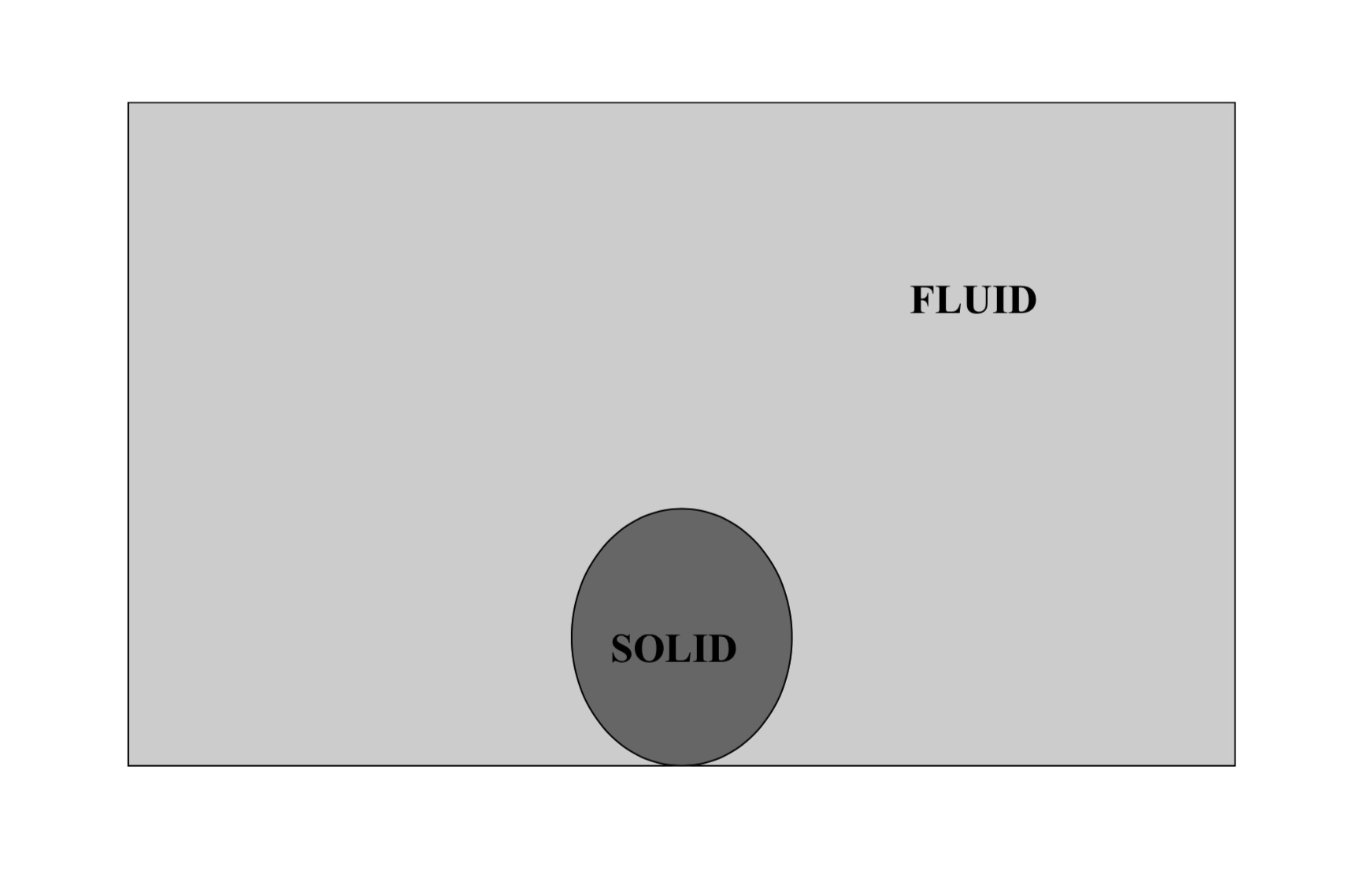
(a) Body touching the container walls.

(b) Cuspidal subregion generated after touching.

Figure 1. The fluid geometry in the presence of collisions.

We begin by recalling the notion of bounded deformation. Let $\Omega\subset\mathbb{R}^{N}$ be a bounded open set. In applications, $N=2,3$. We consider a vector-function $\ \mathbf{v:x}\in\Omega\rightarrow\mathbb{R}^{N}$, and define the tensor of deformation $\mathbb{D}\mathbf{v}=\frac{1}{2}(\nabla\mathbf{v}+\left(\nabla\mathbf{v}\right)^{T})$ with components

$$d{{}_{ij}(}\mathbf{v})=\frac{1}{2}\left(\frac{\partial v_{i}}{\partial x_{j}}+\frac{\partial v_{j}}{\partial x_{i}}\right),\qquad i,j=1,...N.$$

Definition 1.1.

Given $p\geq 1$, we define the space of functions with $L^{p}$-bounded deformation as

$$LD^{p}(\Omega)=\left\{\mathbf{v}\in L^{p}(\Omega):\,\mathbb{D}\mathbf{v}\in L^{p}(\Omega)\right\},$$

endowed by the norm $\ ||\mathbf{v}||_{LD^{p}(\Omega)}=||\mathbf{v}||_{L^{p}(\Omega)}+||\mathbb{D}\mathbf{v}||_{L^{p}(\Omega)}.$

Our main motivation is the validation of the convective term in the Navier - Stokes equations for the fluid-structure interaction problem in the presence of collisions

(1) $$\int_{\Omega}(\mathbf{u}\otimes\mathbf{u}):\mathbb{D}\bm{\psi}\,d\mathbf{x\qquad}\text{for a test function\quad\ }\bm{\psi}\in LD^{2}(\Omega)$$

in cuspidal domains $\Omega$  (see the definition 2.1 in [9]). The convective term is then well defined as a distribution, if the solution $\mathbf{u}\in LD^{2}(\Omega)$ belongs at least to $L^{4}(\Omega)$.

We briefly review existing embedding results for domains with cusps. There are well known embedding results involving the Sobolev space $W_{2}^{1}(\Omega)$ when $\Omega$ has cusps (see [1], [18], [26]).  However, the methods used in these works can not be applied in the case of $LD^{2}(\Omega)$ if one wants a bound on the norm in $LD^{2}(\Omega)$.  The optimal embedding theorem $\,W_{2}^{1}(V(x^{\alpha}))\hookrightarrow L^{r}(V(x^{\alpha}))\,$ for $r\in[1,\frac{2(\alpha+1)}{\alpha-1}]\,$ in the cuspidal domain

$$V(x^{\alpha})=\left\{\mathbf{x}=(x,y):\leavevmode\nobreak\ 0<x<1,\quad 0<y<x^{\alpha}\right\}\subset\mathbb{R}^{2}$$

was obtained in [25]. The embedding result $\,W_{2}^{1}(V(x^{\alpha}))\hookrightarrow L^{q}(\partial V(x^{\alpha})),\,$ with $\,\,1\leqslant q\leqslant 2\,$ for optimal values of $\alpha:\,\,\alpha<1+\frac{2}{q},\,$ was proved in [2]. For a more complete description of optimal embedding results in cuspidal domains, we refer to [7], [22], [24], [26] and [37].

We will show next with an example that knowing $\mathbf{u}\in LD^{2}(\Omega)$ is not enough to guarantee that the convective term in Equation (1) is well defined and additional hypotheses are needed.

Example 1.2.

We consider the cusp domain $V(x^{2})$. This type of cusp appears at the moment in which a solid disk collides with a flat walls in two space dimensions. We take the vector function

(2) $$\mathbf{w}_{s}=((s-1)yx^{-s},x^{1-s})$$

with $s$ a real parameter to be chosen later on. One can compute the associated deformation tensor

$${\mathbb{D}}\mathbf{w}_{s}=\left[\begin{array}[]{cc}-s(s-1)yx^{-s-1}&0\\ 0&0\end{array}\right]$$

as in [3], p. 219-221, from which it follows that

$$||{\mathbb{D}}\mathbf{w}_{s}||_{L^{2}(V(x^{2}))}^{2}\leq C\int_{0}^{1}x^{6-2(s+1)}dx,$$

for some positive constant $C$. Similarly, given $q\geq 1$, we calculate

$$||\mathbf{w}_{s}||_{L^{q}(V(x^{2}))}^{q} \simeq C\int_{0}^{1}\left(\int_{0}^{x^{2}}(y^{q}x^{-qs}+x^{-q(s-1)})\,dy\right)\,dx\simeq C\int_{0}^{1}x^{-q(s-1)+2}\,dx.$$

Consequently,

$$\mathbf{w}_{s}\in LD^{2}(V(x^{2}))\qquad\text{for any}\quad s<1+\frac{3}{2}.$$

Taking $q=2+\varepsilon$, $\varepsilon>0$, we conclude at the same time that

$$\mathbf{w}_{s}\notin L^{2+\varepsilon}(V(x^{2}))\qquad\text{for}\quad s=1+\frac{3}{2+\varepsilon}.$$

In this case, in particular, we cannot make sense of the convective term in Equation (1).

For the applications we have in mind, additional information is available on the integrability of the trace of the function at the boundary. The theory of sets of finite perimeter, which covers most cusp domains, provides a suitable framework for defining the trace on rough (non-Lipschitz) boundaries.

We informally define the space $LD_{\gamma}^{p}(\Omega)$, $1\leq p<\infty$, of functions with $p$th-integrable deformation tensor on $\Omega$ and with $p$th-integrable trace value on the essential boundary of $\Omega$ (see Definition 2.8). Then, our main result is the following embedding result.

Main Result.

Let $\Omega\subset\mathbb{R}^{N}$ be a bounded open set with finite perimeter. Then, there is a continuous embedding

$$LD_{\gamma}^{p}(\Omega)\hookrightarrow L^{\frac{pN}{(N-1)}}(\Omega).$$

In the case $p=2$, $N=2$, we therefore have that $\mathbf{u}\in L^{4}(\Omega)$, as required to define the convective term of Equation (1).

The paper is organized as follows. In Section 2, we recall principal facts about sets of finite perimeters and functions of bounded deformation. We also discuss a few preliminary results needed in the proof of our main theorem, which is presented in Section 3. Throughout, we use standard notation for classical spaces, such as the Sobolev spaces $W^{k,p}(\Omega)$.

Acknowledgments

The second author was partially supported by the US National Science Foundation grant DMS-1615457. The second author acknowledges the hospitality of the Department of Mathematics at the University of Lisbon, where part of this work was conducted.

2. Sets of finite perimeters and bounded deformation

In this section, we briefly recall the needed results on sets of finite perimeter, and states key properties of functions of bounded deformation on such sets. We will use the notation and results in [4], [23], [35] and [36].

We denote the $d$-dimensional Lebesgue measure by $\mathcal{L}^{d}$ and the Hausdorff measure for $d$-dimensional sets in $\mathbb{R}^{N}$, $N\geq d$, as $\mathcal{H}^{d}$. We also denote the space of functions of bounded variation in $\mathbb{R}^{N}$ by $BV(\mathbb{R}^{N})$.

Definition 2.1.

Let $E\subset\mathbb{R}^{N}$ be a bounded $\mathcal{L}^{N}-$measurable set. We denote the characteristic function of the set $E$ by $\chi_{E}$.  If $\chi_{E}\in BV(\mathbb{R}^{N}),$ then $E$ is called a set with finite perimeter. The finite positive number

$$P(E)=|\nabla\chi_{E}|(\mathbb{R}^{N})=\sup_{\mathbf{\phi}}\left\{\int_{E}div\,\mathbf{\phi}\,d\mathbf{x}:\quad|\mathbf{\phi}|\leq 1,\quad\mathbf{\phi}\in C_{c}^{1}(\mathbb{R}^{N})\right\}$$

is called the perimeter of the set $E$.

In the definition above, we have used that, if $\chi_{E}\in BV(\mathbb{R}^{N}),$ then the generalized gradient $\ \nabla\chi_{E}=(\mu_{1},...,\mu_{N})=\mathbf{\mu}$  is a vector with components given by bounded Radon measures $\mu_{i},$ $\ i=1,...N,$ satisfying

$$\int_{E}div\,\mathbf{\phi}\,d\mathbf{x}=-\int_{\mathbb{R}^{N}}(\mathbf{\phi},d\mathbf{\mu)},\qquad\text{for any }\mathbf{\phi}=(\phi_{1},...,\phi_{N})\in C_{c}^{1}(\mathbb{R}^{N}).$$

The following results are discussed in [35, pages 154-156] and in [4, page 159, Proposition 3.62], for instance.

Proposition 2.2.

The following holds

1. The set of all sets with finite perimeter forms algebra, that is, if $E,F$ have finite perimeter then the sets $\mathbb{R}^{N}\backslash E,\,E\cup F,$ $E\cap F$ also have finite perimeter.

2. If $E$ is a Lipschitz domain, then $E$ is a set with finite perimeter and $P(E)=\mathcal{H}^{N-1}(\partial E).$

Remark 2.3.

If we consider the motion of finitely-many rigid bodies in a solid container, all with Lipschitz boundaries, an hypothesis which covers situation of physical and computational interest, then the domain occupied by the fluid will be a set of finite perimeter at all times by Proposition 2.2. (See Figure 2.)

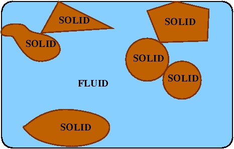
Figure 2. Solid bodies immersed in a fluid in a rigid container.

We introduce the concept of essential boundary for a measurable set (see e.g. [35, pages 256, 258], [5, page 158]). We shall denote the ball of radius $\rho>0$ and center $\mathbf{x}\in\mathbb{R}^{N}$ by $B_{\rho}(\mathbf{x})$, and its volume by $\omega_{N}(\rho)=\mathcal{L}^{N}(B_{\rho}(\mathbf{x}))$. We shall also define the unit sphere

$$\mathbb{S}^{N-1}=\{\mathbf{a}\in\mathbb{R}^{N}:\;\;|\mathbf{a}|=1\}$$

and the hyperplane

$$P_{\mathbf{a}}=\{\mathbf{y}\in\mathbb{R}^{N}:\mathbf{y}\cdot\mathbf{a}=0\}$$

through the origin with normal vector $\mathbf{a}$ in $\mathbb{S}^{N-1}.$ We shall also need the line $l_{\mathbf{a}}(\mathbf{x})$ with direction vector $\mathbf{a}\in\mathbb{S}^{N-1}$ through $\mathbf{x}\in P_{\mathbf{a}}.$

Definition 2.4.

Let $E$ be a given measurable subset of $\mathbb{R}^{N}.$ A point $\mathbf{x\in}E$ is point of density (respectively rarefaction) of the set $E$ if

$$\lim_{\rho\rightarrow 0^{+}}\frac{\mathcal{L}^{N}(E\cap B_{\rho}(\mathbf{x}))}{\omega_{N}(\rho)}=1\quad(\text{respectively}=0).$$

We denote by $E_{\ast}$ the set of all points of density of $E$ and by $E^{\ast}$ the complement of the set of points of rarefaction of $E.$ The set  $\partial^{\ast}E=E^{\ast}\backslash E_{\ast}$ is then called the essential boundary of $E$.

We next recall some facts about the essential boundary for sets with finite perimeter.  For more details we refer the reader to [5], [11], [12], [17], [36], and [38].

Proposition 2.5.

Let $E$ be a set with finite perimeter and let $\partial^{\ast}E$ be its essential boundary. Then

1. The boundary $\partial^{\ast}E$ is countably $\mathcal{H}^{N-1}$-rectifiable, that is,

   $$\partial^{\ast}E=\cup_{n=1}^{\infty}K_{n}\cup S,$$

   where $\mathcal{H}^{N-1}(S)=0$, the sets $K_{n}$ are pairwise disjoint, and each $K_{n}$ is a compact subset of a $C^{1}$ hypersurface in $\mathbb{R}^{N}$

   $$K_{n}=\Phi_{n}(A_{n})$$

   for a compact subset $A_{n}\subset\mathbb{R}^{N-1}$ and a $C^{1}$ map $\Phi_{n}:\mathbb{R}^{N-1}\rightarrow\mathbb{R}^{N}$ [11, page 205].

2. the unit normal $\bm{\nu}=\bm{\nu}(\mathbf{x})$ exists for $\mathcal{H}^{N-1}-$a.a. points $\mathbf{x}\in\partial^{\ast}E$   [11, page 205], [36, pages 227-228], [5, pages 154, 158].

3. Let $\mathbf{a}\in\mathbb{S}^{N-1}$. For $\mathcal{L}^{N-1}$-a.a. $\mathbf{x}\in P_{\mathbf{a}}$, the set $l_{\mathbf{a}}(\mathbf{x})\cap E_{\ast}$ is the union of a finite number of open intervals with disjoint closures, and the union of the boundary points of the intervals coincides with the set $l_{\mathbf{a}}(\mathbf{x})\cap\partial^{\ast}E$   [36, page 233].

In what follows, we denote by $BD(\Omega)$ the space of functions with bounded deformation on $\Omega$ in analogy with $BV(\Omega)$. For $p\geq 1$ the space $LD^{p}(\Omega)$ is a subspace $BD(\Omega)$. Hence, we can apply the result of [33, 34], showing that the trace of functions in $LD^{p}(\Omega)$ is well defined. (The same result was also described carefully in [6, Proposition 4.1].)

Proposition 2.6.

Let $\Omega$ be a set with finite perimeter and let $\partial^{\ast}\Omega$ be its essential boundary.  Let $\mathbf{u}(\mathbf{x})\in LD^{p}(\Omega)$. Then for $\mathcal{H}^{N-1}-$a.e. $\mathbf{x}\in\partial^{\ast}\Omega$, there exist a vector $\gamma\mathbf{u}(\mathbf{x})\in\mathbb{R}^{N}$, such that

(3) $$\lim_{\rho\rightarrow 0^{+}}\frac{2}{\omega_{N}(\rho)}\int_{B_{\rho}(\mathbf{x},\bm{\nu})\cap\Omega}|\mathbf{u}(\mathbf{y})-\gamma\mathbf{u}(\mathbf{x})|\,d\mathbf{y}=0$$

where $\bm{\nu}=\bm{\nu}(\mathbf{x})\in\mathbb{S}^{N-1}$ is the internal normal at $\mathbf{x}\in\partial^{\ast}\Omega$  and the half ball $B_{\rho}(\mathbf{x},\bm{\nu})$ is defined as

(4) $$B_{\rho}(\mathbf{x},\bm{\nu})=\{\mathbf{y}\in\mathbb{R}^{N}:\quad|\mathbf{y}-\mathbf{x}|<\rho,\quad(\mathbf{y}-\mathbf{x})\cdot\bm{\nu}\,>0\}.$$

The assignment $\mathbf{x}\mapsto\gamma\mathbf{u}(\mathbf{x})$ defines a trace map on the essential boundary of $\Omega$ for elements of $LD^{p}(\Omega)$.

We study next the integrability properties of the trace map. If $\Omega$ is a Lipschitz domain, then the embedding $LD^{2}(\Omega)\hookrightarrow L^{2}(\partial\Omega)$ can be established using the same approach of Theorem 1.1 in [33, page 117] and Theorem 3.2 in [6] (see also the theorem and example given on pages 224-227 of [35]). For cusp domains, the above result is generally not true, as the function introduced in Example 1.2 shows.

Example 2.7.

We consider again the function $\mathbf{w}_{s}$ defined in Equation (2) on the cusp domain $V(x^{2})$. This function belongs to $LD^{2}(V(x^{2}))$ for any given $s<1+\frac{3}{2}.$ We then fix

$$s\in[\frac{3}{2},1+\frac{3}{2}),$$

and calculate the $L^{2}$ norm of $\mathbf{w}_{s}$ along the part of the boundary defined by $0<x<1,\quad y=0$

$$\int_{0}^{1}x^{-2(s-1)}dx=+\infty,$$

that is, $\mathbf{w}_{s}\notin L^{2}(\partial V(x^{2}))$. We conclude that the inclusion

$$\qquad LD^{2}(\Omega)\hookrightarrow L^{2}(\partial\Omega)$$

is not valid if $\Omega$ has cusps.

The above example also shows, however, that there can be functions in $LD^{2}(\Omega)$ with square-integrable trace on the essential boundary, even if $\Omega$ is rough (take $\mathbf{w}_{s}$ with $s$ small enough). This observation justifies the introduction of the following space.

Definition 2.8.

Let $\Omega\subset\mathbb{R}^{N}$ be a bounded open set with finite perimeter. Let $LD_{\gamma}^{p}(\Omega)$ be the space of functions $\mathbf{u}\in LD^{p}(\Omega)$ such that the trace of $\mathbf{u}$, $\gamma\mathbf{u}$, defined by Equation (3), is $p$th-integrable on the essential boundary $\partial^{\ast}\Omega$ with respect of Hausdorff measure $\mathcal{H}^{N-1}$.  The space $LD_{\gamma}^{p}(\Omega)$ is a normed vector space with norm

$$\left\|\mathbf{u}\right\|_{LD_{\gamma}^{p}(\Omega)}^{p}=\int_{\Omega}|\mathbb{D}\mathbf{u|}^{p}\,d\mathbf{x}+\int_{\partial^{\ast}\Omega}|\gamma\mathbf{u|}^{p}\,d\mathcal{H}^{N-1}(\mathbf{x}).$$

Remark 2.9.

The space $LD_{\gamma}^{2}(\Omega)$ appears naturally in the construction of the weak solutions to the problem of motion of rigid bodies in a viscous fluid under Navier slip conditions. We refer to the a priori estimate (2.8) established in Theorem 2.1 of [9] (see also the a priori estimate (4.5) in Theorem 1 of [14]).

Our main result is based on an extension of the Fundamental Theorem of Calculus on sections, valid for functions with integrable variation in $W^{1,p}$, to functions with integrable deformation in $LD^{p}$. To this end, we introduce the following notation. For given $\mathbf{a}\in\mathbb{S}^{N-1}$  we define the section

$$\Omega_{\mathbf{y},\mathbf{a}}=\left\{t\in\mathbb{R}:\mathbf{y}+t\mathbf{a}\,\in\Omega\right\}$$

of $\Omega$ corresponding to a point $\mathbf{y}\in P_{\mathbf{a}}(\subset\mathbb{R}^{N-1}).$  If $\Omega_{\mathbf{y},\mathbf{a}}$ is empty, we set

$$\int_{\Omega_{\mathbf{y},\mathbf{a}}}f(\mathbf{y}+t\mathbf{a})\ dt=0$$

for any $\mathcal{L}^{N}-$integrable function $f:\Omega\rightarrow\mathbb{R}$. Then the Fubini-Tonelli theorem implies that

(5) $$\int_{\Omega}f(\mathbf{x})\,d\mathbf{x}=\int_{P_{\mathbf{a}}}\left(\int_{\Omega_{\mathbf{y},\mathbf{a}}}f(\mathbf{y}+t\mathbf{a})\ dt\right)d\mathcal{L}^{N-1}(\mathbf{y)}.$$

The following result, showing absolute continuity on lines, is an analogue of Theorems 7.13 and 10.35 in [23].

Proposition 2.10.

Let $\Omega\subset\mathbb{R}^{N}$  be an open set. Let $\mathbf{a}_{k}\in\mathbb{S}^{N-1},$  $k=1,...,N,$ be arbitrary linearly independent vectors.

For given $\mathbf{u}\in LD^{p}(\Omega)$ there exists a representative $\overline{\mathbf{u}}$ of $\mathbf{u},$ such for each $k=1,...,N$ and $\mathcal{L}^{N-1}$- a.e. $\mathbf{y}\in\mathbb{R}^{N-1}$ the function

$$v_{k}(t)=\mathbf{a}_{k}\,\cdot\overline{\mathbf{u}}(\mathbf{y}+t\mathbf{a}_{k})$$

is absolutely continuous on $t\in\Omega_{\mathbf{y},k}=\Omega_{\mathbf{y},\mathbf{a}_{k}}$ and the following formula

(6) $$v_{k}(t)=v_{k}(t^{\prime})+\int_{t^{\prime}}^{t}\mathbf{a}_{k}\mathbb{D}\mathbf{u}(\mathbf{y}+s\mathbf{a}_{k})\cdot\mathbf{a}_{k}\,\ ds$$

is valid for any $[t^{\prime},t]\subset\Omega_{\mathbf{y},k}.$

Proof.

We consider a sequence of standard mollifiers $\{\varphi_{\varepsilon}\}_{\varepsilon>0}$ (see C.4, pages 552-560, of [23]), and for every $\varepsilon>0$ define

$$\mathbf{u}^{\varepsilon}=\mathbf{u}\ast\varphi_{\varepsilon}\qquad\text{on \quad}\Omega_{\varepsilon}=\left\{\mathbf{x}\in\Omega:\leavevmode\nobreak\ dist(\mathbf{x},\partial\Omega)>\varepsilon\right\}.$$

By the same approach as in Lemma 10.16 of [23], we have

$$\lim_{\varepsilon\rightarrow 0^{+}}\int_{\Omega_{\varepsilon}}\left(|\mathbf{u}^{\varepsilon}-\mathbf{u}|^{p}\,+|\mathbb{D}\mathbf{u}^{\varepsilon}-\mathbb{D}\mathbf{u}|^{p}\right)\,d\mathbf{x}=0.$$

Using (5), it follows that

$$\int_{P_{k}}\left(\int_{\Omega_{\mathbf{y},k}}|\mathbb{D}\mathbf{u}(\mathbf{y}+t\mathbf{a}_{k})|^{p}\,dt\right)\ d\mathcal{L}^{N-1}(\mathbf{y)} < \infty,$$

$$\lim_{\varepsilon\rightarrow 0^{+}}\int_{P_{k}}\left(\int_{(\Omega_{\varepsilon})_{\mathbf{y},k}}|\mathbb{D}\mathbf{u}^{\varepsilon}(\mathbf{y}+t\mathbf{a}_{k})-\mathbb{D}\mathbf{u}(\mathbf{y}+t\mathbf{a}_{k})|^{p}\,dt\right)\ d\mathcal{L}^{N-1}(\mathbf{y)} = 0.$$

Therefore, there exists a subsequence $\{\varepsilon_{n}\},$ such that for $\mathcal{L}^{N-1}-$a.a. $\mathbf{y}\in P_{k}$, $k=1,...,N,$  we have

$$\int_{\Omega_{\mathbf{y},k}}|\mathbb{D}\mathbf{u}(\mathbf{y}+t\mathbf{a}_{k})|^{p}\,dt < \infty,$$

(7) $$\lim_{\varepsilon_{n}\rightarrow 0^{+}}\int_{(\Omega_{\varepsilon_{n}})_{\mathbf{y},k}}|\mathbb{D}\mathbf{u}^{\varepsilon_{n}}(\mathbf{y}+t\mathbf{a}_{k})-\mathbb{D}\mathbf{u}(\mathbf{y}+t\mathbf{a}_{k})|^{p}\,dt = 0.$$

If we set $\mathbf{u}^{{}_{n}}=\mathbf{u}^{\varepsilon_{n}},$ then the sequence $\left\{\mathbf{u}_{n}\right\}$ converges point-wise to $\mathbf{u}$  for $\mathcal{L}^{N}-$ a.a. points of $\Omega$ by Theorem C.19 and Corollary B.122 of [23]. Therefore, the set

$$E=\{\mathbf{x}\in\Omega:\leavevmode\nobreak\ \lim_{n\rightarrow\infty}\mathbf{u}^{{}_{n}}(\mathbf{x})\text{ \ exists in \ }\mathbb{R}^{N}\}$$

is well defined and such that $\mathcal{L}^{N}(\Omega\backslash E)=0.$ We let

$$\overline{\mathbf{u}}(\mathbf{x})=\left\{\begin{array}[]{ll}\lim_{n\rightarrow\infty}\mathbf{u}^{{}_{n}}(\mathbf{x}),&\text{if }\mathbf{x}\in E;\\ 0,&\text{if }\mathbf{x}\in\Omega\backslash E\end{array}\right.$$

and the function $\overline{\mathbf{u}}$ is one of the representatives the equivalence class of $\mathbf{u}$.  Fubini’s theorem implies that

$$\int_{P_{k}}\mathcal{L}^{1}(\left\{t\in\mathbb{R}:\quad\mathbf{y}+t\mathbf{a}_{k}\notin E\,\right\}\cap\Omega_{\mathbf{y},k})\,\ d\mathcal{L}^{N-1}(\mathbf{y)}=0.$$

Thus for $\mathcal{L}^{N-1}-$a.a. $\mathbf{y}\in P_{k}$,

(8) $$\mathbf{y}+t\mathbf{a}_{k}\in E\quad\text{for}\quad\mathcal{L}^{1}-\text{a.a. \ }t\in\Omega_{\mathbf{y},k},\text{ \quad}\forall k=1,...,N.$$

We denote a generic $N$-dimensional rectangle with the edges parallel to the vectors $\mathbf{a}_{1},...,\mathbf{a}_{N}$ in $\mathbb{R}^{N}$ by

$$\mathbb{A}=\left\{\mathbf{x}=\sum_{i,j=1}^{N}t_{k}\,\mathbf{a}_{k}:\quad t_{k}\in[c_{k},d_{k}]\subset\mathbb{R},\text{\quad}\forall k=1,...,N\right\}.$$

We take rectangles $\mathbb{A}\subset\Omega$  with $c_{k},d_{k}$ all rational numbers. For $\varepsilon>0$ sufficiently small, $\mathbb{A}\subset\Omega_{\varepsilon},$ so that by (7) we have that for $\ \mathcal{L}^{N-1}-$a.a.  $\mathbf{y}\in P_{k}$

$$\int_{c_{k}}^{d_{k}}|\mathbb{D}\mathbf{u}(\mathbf{y}+t\mathbf{a}_{k})|^{p}\,dt < \infty,$$

(9) $$\lim_{n\rightarrow\infty}\int_{c_{k}}^{d_{k}}|\mathbb{D}\mathbf{u}^{n}(\mathbf{y}+t\mathbf{a}_{k})-\mathbb{D}\mathbf{u}(\mathbf{y}+t\mathbf{a}_{k})|^{p}\ dt = 0.$$

For each $k=1,...,N$ and$\ \mathcal{L}^{N-1}-$a.a.  $\mathbf{y}\in P_{k},$ we define

$$v_{k}^{n}(t)=\mathbf{u}^{n}(\mathbf{y}+t\mathbf{a}_{k})\cdot\mathbf{a}_{k},\ \text{ \quad}t\in[c_{k},d_{k}].$$

Using (8) we can choose $t^{\prime}\in[c_{k},d_{k}]$ such that $\mathbf{y}+t^{\prime}\mathbf{a}_{k}\,\in E.$  Then, the following limit exists

(10) $$v_{k}^{n}(t^{\prime})\underset{n\rightarrow\infty}{\longrightarrow}v_{k}(t^{\prime})=\overline{\mathbf{u}}(\mathbf{y}+t^{\prime}\mathbf{a}_{k})\cdot\mathbf{a}_{k}.$$

Since $v_{k}^{n}\in C^{\infty}([c_{k},d_{k}]),$ we have

$$v_{k}^{n}(t) = v_{k}^{n}(t^{\prime})+\int_{t^{\prime}}^{t}\frac{d}{ds}\left(v_{k}^{n}(s)\right)\ ds$$

$$= v_{k}^{n}(t^{\prime})+\int_{t^{\prime}}^{t}\sum_{i,j=1}^{N}a_{i}a_{j}d_{ij}(\mathbf{u}^{n}(\mathbf{y}+s\mathbf{a}_{k}))\ ds\qquad\text{for all}\quad t\in[c_{k},d_{k}].$$

Hence, (9)-(10) imply the existence of the limit

$$\lim_{n\rightarrow\infty}v_{k}^{n}(t)=\overline{\mathbf{u}}(\mathbf{y}+t^{\prime}\mathbf{a}_{k})\cdot\mathbf{a}_{k}+\int_{t^{\prime}}^{t}\mathbf{a}_{k}\mathbb{D}\mathbf{u}(\mathbf{y}+s\mathbf{a}_{k}\,)\cdot\mathbf{a}_{k}\ ds,\quad\quad\forall t\in[c_{k},d_{k}].$$

The definition of $E$ and $\overline{\mathbf{u}}$ give then that, for each $k=1,...,N$  and$\ \ \mathcal{L}^{N-1}-$a.a.  $\mathbf{y}\in P_{k},$

(11) $$\left\{\mathbf{y}+t\mathbf{a}_{k}\,:\quad\forall t\in[c_{k},d_{k}]\right\}\subset E$$

(compare with (8)) and the functions $v_{k}(t)=\mathbf{a}_{k}\,\cdot\overline{\mathbf{u}}(\mathbf{y}+t\mathbf{a}_{k}\,)$  satisfy

(12) $$v_{k}(t)=v_{k}(t^{\prime}\mathbf{)}+\int_{t^{\prime}}^{t}\mathbf{a}_{k}\mathbb{D}(\mathbf{u}(\mathbf{y}+s\mathbf{a}_{k}))\cdot\mathbf{a}_{k}\,ds,\quad\quad\forall t\in[c_{k},d_{k}].$$

Consequently, each function $v_{k}\mathbf{=}v_{k}(t)$ is absolutely continuous on $[c_{k},d_{k}]$ and

$$\frac{dv}{dt}(t)=\mathbf{a}_{k}\mathbb{D}(\mathbf{u}(\mathbf{y}+t\mathbf{a}_{k}))\cdot\mathbf{a}_{k}\qquad\text{for \ }\mathcal{L}^{1}\text{ - a.e.}\quad t\in[c_{k},d_{k}],$$

which can be shown as in Lemma 3.31 of [23].

Now, if $\widetilde{\mathbb{A}}\subset\Omega$ is another such rectangle with the property that

$$[c_{k},d_{k}]\cap[\widetilde{c}_{k},\widetilde{d}_{k}]\neq\varnothing,\text{\quad}\forall k=1,...,N,$$

then, by taking $\mathbf{y}\in P_{k}$, which is admissible for both $\mathbb{A}$ and $\widetilde{\mathbb{A}}$,  and $\ t^{\prime}\in[c_{k},d_{k}]\cup[\widetilde{c}_{k},\widetilde{d}_{k}],$ it follows that from (11) and (12) that $v_{k}$ is absolutely continuous on the interval $[c_{k},d_{k}]\cup[\widetilde{c}_{k},\widetilde{d}_{k}].$

Since $\Omega$ can be written as a countable union of closed rectangles of this type and since the union of countably many sets of $\mathcal{L}^{N-1}$-measure zero still has $\mathcal{L}^{N-1}$-measure zero, using (11), (12) we conclude that for $\mathcal{L}^{N-1}$-a.e. $\mathbf{y}\in P_{k}$,  the function $v_{k}(t)$  is absolutely continuous on any connected component of $\Omega_{\mathbf{y},k}$. ∎

Next, we formulate and prove a result concerning a non-tangential approach to characterize the trace. In what follows, we let $\Omega$ be an open set of finite perimeter. We recall that $\bm{\nu}=\bm{\nu}(\mathbf{x})\in\mathbb{S}^{N-1}$ denotes the internal normal at $\mathbf{x}\in\partial^{\ast}\Omega$ and $B_{1}(\mathbf{x},\bm{\nu})$ is the half ball with radius equal 1, defined by (4).

Let $\mathbf{a}\in\mathbb{S}^{N-1}\cap B_{1}(\mathbf{x},\bm{\nu})$ be arbitrary fixed vector and set

(13) $$\lambda_{\mathbf{a}}(E)=\mathcal{L}^{N-1}(\pi_{\mathbf{a}}E)$$

for any measurable (Borel) set $E\subset\mathbb{R}^{N}$, where $\pi_{\mathbf{a}}E$ is the projection of the set $E\subset\mathbb{R}^{N}$ onto the plane $P_{\mathbf{a}}$. (We refer to [36, pages 235-236] for a discussion of properties of the Borel measure $\lambda_{\mathbf{a}}$.)

Proposition 2.11.

Let $\mathbf{u}\in LD_{\gamma}^{p}(\Omega)$. The following limit exists

(14) $$\gamma_{\mathbf{a}}\mathbf{u}(\mathbf{x})=\lim_{\varepsilon\rightarrow 0^{+}}\frac{1}{\varepsilon}\int_{0}^{\varepsilon}\mathbf{u}(\mathbf{x}+s\mathbf{a})\,ds\qquad\text{for\quad}\lambda_{\mathbf{a}}-a.e.\quad\mathbf{x}\in\partial^{\ast}\Omega,$$

such that

(15) $$\gamma_{\mathbf{a}}\mathbf{u}(\mathbf{x})=\gamma\mathbf{u}(\mathbf{x})\qquad\text{for\quad}\lambda_{\mathbf{a}}-a.e.\quad\mathbf{x}\in\partial^{\ast}\Omega.$$

We omit the proof Proposition 2.11, as it is essentially the same as that of Theorem in Section 11.2, pages 243-245, of [36]. In fact the proof of this above-mentioned theorem relies on the structure of the set with finite perimeter and the existence of the trace values $\gamma\mathbf{u}$ for a given function $\mathbf{u}.$ In our case, when $\mathbf{u}\in LD_{\gamma}^{p}(\Omega)$,  the existence of $\gamma\mathbf{u}$ is guaranteed by Proposition 2.6.

Corollary 2.12.

Let $\Omega\subset\mathbb{R}^{N}$  be an open set of finite perimeter. Then under the assumptions and the notation of Proposition 2.10, Formula (6) is valid for any $t^{\prime},t\in\mathbb{R},$ such that

$$[t^{\prime},t]\subset\overline{\Omega_{\mathbf{y},k}}.$$

Proof.

By Proposition 2.10 we have that for $\mathcal{L}^{N-1}$- a.e. $\mathbf{y}\in P_{\mathbf{a}_{k}},$

(16) $$v_{k}(t)=v_{k}(t^{\prime})+\int_{t^{\prime}}^{t}\mathbf{a}_{k}\mathbb{D}\mathbf{u}(\mathbf{y}+s\mathbf{a}_{k})\cdot\mathbf{a}_{k}\ ds\qquad\text{for any \ }[t^{\prime},t]\subset\Omega_{\mathbf{y},k}\text{.}$$

Moreover, there exists a finite number of disjoint intervals $[t_{0}^{\prime},t_{0}]$, such that

$$t_{0}^{\prime}\neq t_{0},\text{\qquad}[t_{0}^{\prime},t_{0}]\subset\overline{\Omega_{\mathbf{y},k}}\text{\qquad and\qquad}\mathbf{y}+t_{0}^{\prime}\mathbf{a}_{k},\text{ }\mathbf{y}+t_{0}\mathbf{a}_{k}\in\partial^{\ast}\Omega$$

by Proposition 2.5 (iii).

If we integrate (16) over $t^{\prime}\in(t_{0}^{\prime},,t_{0}^{\prime}+\varepsilon),$ divide by $\varepsilon$, and take the limit $\varepsilon\rightarrow 0,$ then Proposition 2.11 implies that (16) is valid for $t^{\prime}=t_{0}^{\prime}.$ By the same way we can demonstrate the validity of (16) for the point $t=t_{0}$. Combining these identifications with the integral representation for $v_{k}$ above, we obtain Formula (6) for all $[t^{\prime},t]$ in $\overline{\Omega_{\mathbf{y},k}}$. ∎

3. Proof of the main result

We are now ready to prove our main result. We first recall a needed proposition. For a vector $\bm{\xi}=(\xi_{1},\dots,\xi_{N})\in\mathbb{R}^{N}$  and each $i\in\left\{1,\ldots,N\right\}$, we introduce the vectors

(17) $$\widehat{\bm{\xi}}_{i}=(\xi_{1},\dots,\xi_{i-1},\xi_{i+1},...,\xi_{N})\in\mathbb{R}^{N-1}.$$

For a proof of the following proposition, we refer to [33], pages 128-129, Lemma 1.1.

Proposition 3.1.

Let $\theta_{i}=\theta_{i}(\widehat{\bm{\xi}}_{i})$ be non-negative integrable functions in $\mathbb{R}^{N-1}$, $i=1,\ldots,N$. Then,

(18) $$\int_{\mathbb{R}^{N}}\left(\prod_{i=1}^{N}\theta_{i}\right)^{\frac{1}{N-1}}\,d\mathbf{\xi}\leq\prod_{i=1}^{N}\left(\int_{\mathbb{R}^{N-1}}\theta_{i}(\widehat{\bm{\xi}}_{i})\,d\widehat{\bm{\xi}}_{i}\right)^{\frac{1}{N-1}}.$$

The main result of this work is the following theorem.

Theorem 3.2.

Let $\Omega$ be a bounded open set with finite perimeter. If $\mathbf{u}\in LD_{\gamma}^{p}(\Omega)$, then $\mathbf{u}\in L^{\frac{pN}{(N-1)}}(\Omega)$ and there exists a positive constant $C$, depending only on $N$, $p$ and the diameter of the domain $\Omega$, such that

(19) $$\left\|\mathbf{u}\right\|_{L^{\frac{pN}{(N-1)}}(\Omega)}\leq C\left\|\mathbf{u}\right\|_{LD_{\gamma}^{p}(\Omega)}.$$

Proof.

We follow closely the proof in Theorem 1.2, page 117, of [33] and Theorem 6.95, pages 333-336, of [10], and combine them with the ideas developed in the theorem of Section 5, pages 218-220, in [35]. We adapt this approach to the case at hand of sets with finite perimeter.

(I) As a warm-up for the general case, we start by considering two space dimensions and $p=2$. Let $\left\{\mathbf{e}_{1},\mathbf{e}_{2}\right\}$ be the Euclidean basis of $\mathbb{R}^{2}.$ We denote a point in $\mathbb{R}^{2}$ with $\mathbf{x}=(x_{1},x_{2})$ and a vector field on $\mathbb{R}^{2}$ with $\mathbf{u}=(u,v)$.

Step 1: Since the set $\Omega$ has a finite perimeter, then by Part (iii) of Proposition 2.5 for $\mathcal{L}^{1}$-a.a. $x_{2}\in\mathbb{R}$, the intersection

$$\Omega(x_{2})=l_{\mathbf{e}_{1}}((0,x_{2}))\cap\Omega$$

consists of a finite number $M_{2}(x_{2})$ of open intervals with disjoint closures

$$\Omega(x_{2})=\cup_{l=1}^{M_{2}(x_{2})}\triangle_{2,l},\qquad\text{such that}\quad\overline{\triangle_{2,l}}\cap\overline{\triangle_{2,m}}=\varnothing,\quad\forall l\neq m,$$

where $\triangle_{2,l}=(\mathbf{c}_{2,l}(x_{2}),\mathbf{d}_{2,l}(x_{2}))$ is a straight line connecting the points

$$\mathbf{c}_{2,l}(x_{2})=(c_{2,l}(x_{2}),x_{2}),\mathbf{\ \ d}_{2,l}(x_{2})=(d_{2,l}(x_{2}),x_{2})\in\partial^{\ast}\Omega.$$

Consequently, Corollary 2.12 implies that for such admissible $x_{2}\in\mathbb{R}$ and arbitrary chosen $x_{1}\in\Omega(x_{2})$, there exists an index $k\in\left\{1,\ldots,M_{2}(x_{2})\right\}$, such that $x_{1}\in\triangle_{2,k}$ and

$$u\mathbf{(x)}=u(x_{1},x_{2})=\gamma u(\mathbf{c}_{2,k}(x_{2}))+\int_{c_{2,k}(x_{2})}^{x_{1}}\partial_{x_{1}}u(s,x_{2})\ ds.$$

It follows that

$$u^{2}\mathbf{(x)} \leq 2\left[|\gamma u(\mathbf{c}_{2,k}(x_{2}))|^{2}+(d_{2,k}(x_{2})-c_{2,k}(x_{2}))\cdot\right.$$

$$\left.\qquad\qquad\qquad\qquad\qquad\cdot\int_{c_{2,k}(x_{2})}^{d_{2,k}(x_{2})}|\partial_{x_{1}}u(s,x_{2})|^{2}\ ds\right]$$

$$\leq C\sum\limits_{l=1}^{M_{2}(x_{2})}\left[|\gamma\mathbf{u}(\mathbf{c}_{2,l}(x_{2}))|^{2}+\int_{c_{2,l}(x_{2})}^{d_{2,l}(x_{2})}|d_{11}(\mathbf{u})(s,x_{2})|^{2}\ ds\right]$$

(20) $$=f_{2}(x_{2})$$

where the constant $C$ depends only on the diameter of $\Omega.$

In the same fashion, for $\mathcal{L}^{1}$-a.a. $x_{1}\in\mathbb{R}$  the intersection

$$\Omega(x_{1})=l_{\mathbf{e}_{2}}((x_{1},0))\cap\Omega$$

consists of a finite number $M_{1}(x_{1})$ of open intervals with disjoint closures

$$\Omega(x_{1})=\cup_{l=1}^{M_{1}(x_{1})}\triangle_{1,l},\qquad\text{such that}\quad\overline{\triangle_{1,l}}\cap\overline{\triangle_{1,m}}=\varnothing,\quad\forall l\neq m,$$

where $\triangle_{1,l}=(\mathbf{c}_{1,l}(x_{1}),\mathbf{d}_{1,l}(x_{1}))$ is a straight line connecting the points

$$\mathbf{c}_{1,l}(x_{1})=(x_{1},c_{1,l}(x_{1})),\mathbf{\ \ d}_{1,l}(x_{1})=(x_{1},d_{1,l}(x_{1}))\in\partial^{\ast}\Omega.$$

For admissible $x_{1}\in\mathbb{R}$ and arbitrary chosen $x_{2}\in\Omega(x_{1})$, there exists an index $k\in\left\{1,\ldots,M_{1}(x_{1})\right\},$ such that $x_{2}\in\triangle_{1,k}$ and

$$v\mathbf{(x)}=v(x_{1},x_{2})=\gamma v(\mathbf{c}_{1,k}(x_{1}))+\int_{c_{1,k}(x_{1})}^{x_{2}}\partial_{x_{2}}v(x_{1},s)\ ds.$$

Hence

(21) $$v^{2}\mathbf{(x)} \leq C\sum\limits_{l=1}^{M_{1}(x_{1})}\left[|\gamma\mathbf{u}(\mathbf{c}_{1,l}(x_{1}))|^{2}+\int_{c_{1,l}(x_{1})}^{d_{1,l}(x_{1})}|d_{22}(\mathbf{u})(x_{1},s)|^{2}\ ds\right]$$

$$= f_{1}(x_{1}).$$

Multiplying (20) with (21) and integrating over $\Omega,$ by Proposition 3.1 (or simply by the Fubini-Tonelli Theorem) we obtain

$$\int_{\Omega}u^{2}\mathbf{(x)}v^{2}\mathbf{(x)}\ d\mathbf{x}\leq\int_{\Omega}f_{1}(x_{1})f_{2}(x_{2})\ d\mathbf{x}\leq\int_{I_{1}}f_{1}(x_{1})\ dx_{1}\int_{I_{2}}f_{2}(x_{2})\ dx_{2},$$

where $I_{i},$ $i=1,2,$ are the projections of $\Omega$ onto the $x_{i}$-coordinate axis. We have

$$\left.\begin{array}[]{c}\displaystyle{\int_{I_{1}}\sum\limits_{l=1}^{M_{1}(x_{1})}|\gamma\mathbf{u}(\mathbf{c}_{1,l}(x_{1}))|^{2}\ dx_{1}}\\ \\ \displaystyle{\int_{I_{2}}\sum\limits_{l=1}^{M_{2}(x_{2})}|\gamma\mathbf{u}(\mathbf{c}_{2,l}(x_{2}))|^{2}\ dx_{2}}\end{array}\right\}\leq\int_{\partial^{\ast}\Omega}|\gamma(\mathbf{u})\mathbf{|}^{2}\,d\mathcal{H}^{N-1}(\mathbf{x})$$

by the properties of the measure $\lambda_{\mathbf{a}}$ given on the pages 235-236, section 7, of [36]. Therefore,

$$\int_{\Omega}u^{2}\mathbf{(x)}v^{2}\mathbf{(x)}\,d\mathbf{x} \leq C\,\int_{I_{2}}f_{1}(x_{1})\ dx_{1}\int_{I_{1}}f_{2}(x_{2})\ dx_{2}$$

(22) $$\leq C\left(\int_{\partial^{\ast}\Omega}|\gamma(\mathbf{u})\mathbf{|}^{2}\,d\mathcal{H}^{N-1}(\mathbf{x})+\int_{\Omega}|\mathbb{D}\mathbf{u|}^{2}\,d\mathbf{x}\right)^{2}=C\left\|\mathbf{u}\right\|_{LD_{\gamma}^{2}(\Omega)}^{4}.$$

2nd step: Now we consider the basis  $\mathbf{a}_{1}=\frac{1}{\sqrt{2}}(1,1),$  $\mathbf{a}_{2}=\frac{1}{\sqrt{2}}(-1,1).$ We denote the coordinates of $\mathbf{x}$ in the basis $(\mathbf{a}_{1},\mathbf{a}_{2})$ by $(\xi_{1},\xi_{2}),$ that is,

$$\mathbf{x}=(\mathbf{x}_{1},\mathbf{x}_{2})=\xi_{1}\mathbf{a}_{1}+\xi_{2}\mathbf{a}_{2}.$$

Again, for $\mathcal{L}^{1}$- a.e. $\mathbf{y}_{2}=\xi_{2}\mathbf{a}_{2}\in P_{\mathbf{a}_{1}},$ i.e., for $\mathcal{L}^{1}$- a.e. $\xi_{2}\in\mathbb{R}$, the intersection of lines parallel to $\mathbf{a}_{1}$ with the domain $\Omega,$ passing through $\mathbf{y}_{2},$

$$\Omega(\xi_{2})=l_{\mathbf{a}_{1}}(\mathbf{y}_{2})\cap\Omega$$

consists of a finite number $M_{2}(\xi_{2})$ of open intervals with disjoint closures, such that for$\ \mathbf{x}\in\Omega(\xi_{2}),$ there exists an interval

$$(\mathbf{c}_{2,k}(\xi_{2}),\mathbf{d}_{2,k}(\xi_{2}))\subset\Omega(\xi_{2})\qquad\text{with\quad}\mathbf{c}_{2,k}(\xi_{2}),\mathbf{d}_{2,k}(\xi_{2})\in\partial^{\ast}\Omega.$$

For simplicity of notation, we assume that this interval, being a part of $l_{\mathbf{a}_{1}}(\mathbf{y}_{2}),$ is described as

$$(\mathbf{c}_{2,k}(\xi_{2}),\mathbf{d}_{2,k}(\xi_{2}))=\left\{\,\mathbf{y}=\mathbf{y}_{2}+s\mathbf{a}_{1}\in\mathbb{R}^{N}:\leavevmode\nobreak\ s\in(c_{2,k}(\xi_{2}),d_{2,k}(\xi_{2}))\right\}.$$

By applying Corollary 2.12 to the function

$$v_{2}(\xi_{1},\xi_{2})=\mathbf{a}_{1}\,\cdot\mathbf{u}(\mathbf{y}_{2}+\xi_{1}\mathbf{a}_{1})$$

and proceeding as in (20)-(21), we obtain

$$v_{2}^{2} \leq 2\left[|\mathbf{a}_{1}\,\cdot\gamma\mathbf{u}(\mathbf{c}_{2,k}(\xi_{2}))|^{2}\right.$$

$$\qquad\left.+(d_{2,k}(\xi_{2})-c_{2,k}(\xi_{2}))\int_{c_{2,k}(\xi_{2})}^{d_{2,k}(\xi_{2})}|\mathbf{a}_{2}\mathbb{D}\mathbf{u}(\mathbf{y}_{2}+s\mathbf{a}_{1})\cdot\mathbf{a}_{2}|^{2}\ ds\right]$$

$$\leq\sum\limits_{l=1}^{M_{2}(\xi_{2})}\left[|\gamma\mathbf{u}(\mathbf{c}_{2,l}(\xi_{2}))|^{2}+\int_{c_{2,l}(\xi_{2})}^{d_{2,l}(\xi_{2})}|\mathbb{D}\mathbf{u}(\mathbf{y}_{2}+s\mathbf{a}_{1})|^{2}\ ds\right]$$

(23) $$=f_{2}(\xi_{2}).$$

Similarly, for $\mathcal{L}^{1}$- a.e. $\mathbf{y}_{1}=\xi_{1}\mathbf{a}_{1}\in P_{\mathbf{a}_{2}},$ that is, or $\mathcal{L}^{1}$- a.e. $\xi_{1}\in\mathbb{R}$,  the intersection of the line parallel to $\mathbf{a}_{2}$ with $\Omega$ passing through $\mathbf{y}_{1}$

$$\Omega(\xi_{1})=l_{\mathbf{a}_{2}}(\mathbf{y}_{1})\cap\Omega$$

is a finite number $M_{1}(\xi_{1})$ of open intervals with disjoint closures. Then for$\ \mathbf{x}\in\Omega(\xi_{1})$ there exists an interval, such that

$$(\mathbf{c}_{1,k}(\xi_{1}),\mathbf{d}_{1,k}(\xi_{1}))\subset\Omega(\xi_{1})\qquad\text{with\quad}\mathbf{c}_{1,k}(\xi_{1}),\mathbf{d}_{1,k}(\xi_{1})\in\partial^{\ast}\Omega.$$

Defining

$$v_{1}(\xi_{1},\xi_{2})=\mathbf{a}_{1}\,\cdot\mathbf{u}(\mathbf{y}_{1}+\xi_{2}\mathbf{a}_{2}),$$

Corollary 2.12 gives

$$v_{1}^{2}\leq C\sum\limits_{l=1}^{M_{1}(\xi_{1})}\left[|\gamma\mathbf{u}(\mathbf{c}_{1,l}(\xi_{1}))|^{2}+\int_{c_{1,l}(\xi_{1})}^{d_{1,l}(\xi_{1})}|\mathbb{D}\mathbf{u}(\mathbf{y}_{2}+s\mathbf{a}_{1})|^{2}\ ds\right]=f_{1}(\xi_{1}).$$

Multiplying this inequality by (23), integrating over $(\xi_{1},\xi_{2})\in\Omega$, and proceeding as in the derivation of Equation (22), yields

$$\int_{\Omega}v_{2}^{2}v_{1}^{2}\ d\xi_{1}d\xi_{2}\leq C\left\|\mathbf{u}\right\|_{LD_{\gamma}^{2}(\Omega)}^{2}.$$

Observing that

$$\int_{\Omega}v_{2}^{2}v_{1}^{2}\ d\xi_{1}d\xi_{2} = \int_{\Omega}(\mathbf{a}_{1}\cdot\mathbf{u}(\mathbf{x}))^{2}(\mathbf{a}_{2}\cdot\mathbf{u}(\mathbf{x}))^{2}\ d\mathbf{x}$$

$$= \frac{1}{4}\int_{\Omega}(u-v)^{2}(u+v)^{2}\ d\mathbf{x,}$$

we obtain

$$\int_{\Omega}(u^{4}-2u^{2}v^{2}+v^{4})\ d\mathbf{x}\leq C\left\|\mathbf{u}\right\|_{LD_{\gamma}^{2}(\Omega)}^{2}.$$

Therefore, by combining this estimate with estimate (22) we conclude that

$$\|\mathbf{u}\|_{L^{4}(\Omega)}^{4}=\int_{\Omega}(u^{4}+v^{4})\ d\mathbf{x}\leq C\left\|\mathbf{u}\right\|_{LD_{\gamma}^{2}(\Omega)}^{4}.$$

which coincides with (19) for $N=2$ and $p=2.$

(II) We now turn to the general $N$-dimensional case.  We follow closely the proof of Theorem 6.95, pages 333-336, of [10].

We denote the Euclidean basis of $\mathbb{R}^{N}$ by $\{\mathbf{e}_{i}\}_{i=1}^{N}$ .  Given a vector $\mathbf{a}\in\mathbb{S}^{N-1}$ and a point $\mathbf{x}\in\Omega$, we let $\mathbf{y}=\text{Proj}_{\mathbf{a}}\mathbf{x}\in P_{\mathbf{a}}$ be the projection of $\mathbf{x}$ on the plane $P_{\mathbf{a}}$, and we let

$$\Omega_{\mathbf{a}}(\mathbf{y})=l_{\mathbf{a}}(\mathbf{y})\cap\Omega$$

be the intersection of $\Omega$ with the line parallel to $\mathbf{a}$ and crossing $\mathbf{y}$ $($and $\mathbf{x).}$

Since $\Omega$ is, by hypothesis, a set of finite perimeter, for $\mathcal{L}^{N-1}-$a.a. $\mathbf{y}=\text{Proj}_{\mathbf{a}}\mathbf{x}\in P_{\mathbf{a}}$,$\ \ \ \Omega_{\mathbf{a}}(\mathbf{y})$ is a finite number $M_{\mathbf{a}}(\mathbf{y})$ of open intervals with disjoint closures. Consequently, for $\mathcal{L}^{N-1}-$a.a. $\mathbf{y}=\text{Proj}_{\mathbf{a}}\mathbf{x}\in P_{\mathbf{a}}$, the point $\mathbf{x}$ belongs to one of these intervals and its endpoints, which we denote by $\mathbf{c}_{k}(\mathbf{x})$, $\mathbf{d}_{k}(\mathbf{x})$ are on the essential boundary $\partial^{\ast}\Omega$ of $\Omega$. For simplicity of notation, we assume that this interval is described as

$$(\mathbf{c}_{\mathbf{a},k}(\mathbf{y}),\mathbf{d}_{\mathbf{a},k}(\mathbf{y}))=\left\{\,\mathbf{x}\in\mathbb{R}^{N}:\leavevmode\nobreak\ \mathbf{x}=\mathbf{y}+t\mathbf{a},\mathbf{\qquad}t\in(c_{\mathbf{a},k}(\mathbf{y}),d_{\mathbf{a},k}(\mathbf{y}))\right\}.$$

If we consider the function

$$v_{\mathbf{a}}(\mathbf{x})=\mathbf{a}\cdot\mathbf{u}(\mathbf{x})=\sum_{i=1}^{N}a_{i}u_{i}(\mathbf{x}),$$

then Corollary 2.12 implies that

$$|v_{\mathbf{a}}(\mathbf{x})|\leq|\gamma(v_{\mathbf{a}})(\mathbf{c}_{\mathbf{a},k}(\mathbf{y}))|+\int_{c_{\mathbf{a},k}(\mathbf{y})}^{d_{\mathbf{a},k}(\mathbf{y})}|\mathbf{a}\mathbb{D}\mathbf{u}(\mathbf{y}+s\mathbf{a})\cdot\mathbf{a|}\,\ ds.$$

We have the elementary inequalities

$$|\gamma(v_{\mathbf{a}})|\leq C|\gamma\mathbf{u}|,\qquad|\mathbf{a}\mathbb{D}\mathbf{u}(\mathbf{y}+s\mathbf{a})\cdot\mathbf{a}|\leq C|\mathbb{D}(\mathbf{u})|.$$

Here and below $C$ are constants depending only on $N,$ $p$ and the diameter of $\Omega.$ Therefore,

(24) $$|v_{\mathbf{a}}(\mathbf{x})|^{p} \leq C\sum_{l=1}^{M_{\mathbf{a}}(\mathbf{y})}\left(|\gamma\mathbf{u}(\mathbf{c}_{\mathbf{a},l}(\mathbf{y}))|^{p}+\int_{c_{\mathbf{a},l}(\mathbf{y})}^{d_{\mathbf{a},l}(\mathbf{y})}|\mathbb{D}(\mathbf{u})(\mathbf{y}+s\,\mathbf{a})|^{p}\ ds\right)$$

$$= H_{N}(\mathbf{u})(\mathbf{y}),$$

for $\mathcal{L}^{N-1}-$a.a. $\mathbf{y}=\text{Proj}_{\mathbf{a}}\mathbf{x}\in P_{\mathbf{a}}.$

We introduce the orthonormal projections

$$\mathbf{h}_{k}=\frac{\mathbf{a}-a_{k}\,\mathbf{e}_{k}}{|\mathbf{a}-a_{k}\,\mathbf{e}_{k}|}\qquad\text{for each }k=1,2,...,N-1$$

of the vector $\mathbf{a}$ onto the coordinates hyperplanes, identified canonically with $\mathbb{R}^{N-1}$. As in (24), for a fixed $k\in\{1,...,N-1\}$  the function $v_{\mathbf{h}_{k}}(\mathbf{x})=\mathbf{h}_{k}\cdot\mathbf{u}(\mathbf{x})$ satisfies the inequality

(25) $$|v_{\mathbf{h}_{k}}(\mathbf{x})|^{p} \leq C\sum_{l=1}^{M_{\mathbf{h}_{k}}(\mathbf{y}^{\prime})}\left(|\gamma\mathbf{u}(\mathbf{c}_{\mathbf{h}_{k},l}(\mathbf{y}^{\prime}))|^{p}+\int_{c_{\mathbf{h}_{k},l}(\mathbf{y}^{\prime})}^{d_{\mathbf{h}_{k},l}(\mathbf{y}^{\prime})}|\mathbb{D}(\mathbf{u})(\mathbf{y}^{\prime}+s\,\mathbf{h}_{k})|^{p}\ ds\right)$$

$$= I_{k}(\mathbf{u})(\mathbf{y}^{\prime}),$$

for $\mathcal{L}^{N-1}-$a.a. $\mathbf{y}^{\prime}=\text{Proj}_{\mathbf{h}_{k}}\mathbf{x}\in P_{\mathbf{h}_{k}}$. Similarly, the function $v_{\mathbf{e}_{k}}(\mathbf{x})=\mathbf{e}_{k}\cdot\mathbf{u}(\mathbf{x})$ satisfies

(26) $$|v_{\mathbf{e}_{k}}(\mathbf{x})|^{p} \leq C\sum_{l=1}^{M_{\mathbf{e}_{k}}(\mathbf{y}^{\prime\prime})}\left(|\gamma\mathbf{u}(\mathbf{c}_{\mathbf{e}_{k},l}(\mathbf{y}^{\prime\prime}))|^{p}+\int_{c_{\mathbf{e}_{k},l}(\mathbf{y}^{\prime\prime})}^{d_{\mathbf{e}_{k},l}(\mathbf{y}^{\prime\prime})}|\mathbb{D}(\mathbf{u})(\mathbf{y}^{\prime\prime}+s\,\mathbf{e}_{k})|^{p}\ ds\right)$$

$$= J_{k}(\mathbf{u})(\mathbf{y}^{\prime\prime}),$$

for $\mathcal{L}^{N-1}-$a.a. $\mathbf{y}^{\prime\prime}=\text{Proj}_{\mathbf{e}_{k}}\mathbf{x}\in P_{\mathbf{e}_{k}}.$  Keeping $k$ fixed, it follows that

$$v_{\mathbf{a}}(\mathbf{x})=\sum_{i=1}^{N}a_{i}u_{i}(\mathbf{x})=v_{\mathbf{h}_{k}}(\mathbf{x})+a_{k}v_{\mathbf{e}_{k}}(\mathbf{x}).$$

Consequently,

(27) $$|v_{\mathbf{a}}(\mathbf{x})|^{p}\leq C\left[I_{k}(\mathbf{u})(\mathbf{y}^{\prime})+J_{k}(\mathbf{u})(\mathbf{y}^{\prime\prime})\right].$$

We next use estimates (24)-(26) to bound

$$|v_{\mathbf{a}}(\mathbf{x})|^{pN}\leq C\,H_{N}(\mathbf{u})\,\prod_{k=1}^{N-1}\left[I_{k}(\mathbf{u})+J_{k}(\mathbf{u})\right].$$

Using this inequality and the elementary bound

$$\left(\alpha_{1}+...+\alpha_{n}\right)^{1/(N-1)}\leq n^{1/(N-1)}(\alpha_{1}^{1/(N-1)}+...+\alpha_{n}^{1/(N-1)}),$$

which is valid for any positive $\alpha_{1},...,\alpha_{n}$ and for any $n\in\mathbb{N}$ (in particular for $n=2^{N-1}$), one can show that $|v_{\mathbf{a}}(\mathbf{x})|^{pN/(N-1)}$ is bounded by a linear combination of $2^{N-1}$ terms of the form

(28) $$I_{\sigma}=\left(H_{1}\ldots H_{N}\right)^{1/(N-1)},$$

where $H_{k}$ denotes either $I_{k}$ or $J_{k}$.

Each of the terms $H_{k}$ in the product above depends on $N-1$ variables, and hence we can apply Proposition 3.1. To see this fact, we introduce an adapted basis $\{\mathbf{E}_{k}\}_{k=1}^{N}$ as follows. For each index $k\in\{1,\ldots,N-1\}$, we pick a vector $\mathbf{E}_{k}$ belonging to the set $\left\{\mathbf{h}_{k},\mathbf{e}_{k}\right\}$, and for $k=N$, we set $\mathbf{E}_{N}=\mathbf{a}.$ If all components of the vector $\mathbf{a}$ are non zero, it is then easy to see that

$$\{\mathbf{E}_{k}\}_{k=1}^{N-1}\text{\quad is a basis of }\mathbb{R}^{N-1}\text{\qquad and\qquad}\{\mathbf{E}_{k}\}_{k=1}^{N}\text{\quad is a basis of }\mathbb{R}^{N}.$$

For a proof of this fact we refer to Lemma 6.96, page 334-335, of [10]. We let $\xi_{j},$ $j=1,...,N,$ denote the coordinates of $\mathbf{x}\in\mathbb{R}^{N}$ in the basis $\mathbf{E}_{1},...,\mathbf{E}_{N}$, that is,

$$\mathbf{x}=\sum_{j=1}^{N}x_{i}\mathbf{e}_{{}_{j}}=\sum_{j=1}^{N}\xi_{j}\,\mathbf{E}_{j}$$

and identify $\mathbf{x}$ with the vector $\bm{\xi}=\sum_{j=1}^{N}\xi_{j}\,\mathbf{E}_{j}.$

Then, each term $I_{\sigma}$ can be rewritten as

$$(I_{\sigma}(\mathbf{x}(\bm{\xi})))^{N-1}=\prod_{k=1}^{N}\theta_{k}(\widehat{\mathbf{\xi}}_{k}),\;\quad\theta_{k}(\widehat{\bm{\xi}}_{k})=H_{k}(\text{Proj}_{\mathbf{E}_{k}}\mathbf{x}(\bm{\xi})),\;k=1,...,N.$$

Proceeding as in the derivation of (22) gives

$$\int_{\mathbb{R}^{N-1}}\theta_{k}(\widehat{\bm{\xi}}_{k})\,d\widehat{\bm{\xi}}_{k}\leq\left\|\mathbf{u}\right\|_{LD_{\gamma}^{p}(\Omega)}^{p}.$$

By Proposition 3.1 it follows that

(29) $$\int_{\Omega}I_{\sigma}(\mathbf{x})\,d\mathbf{x}\leq C(\sigma)\,\prod_{i=1}^{N}\left(\int_{\mathbb{R}^{N-1}}\theta_{k}\,d\widehat{\bm{\xi}}_{k}\right)^{\frac{1}{N-1}}\leq C\,\left\|\mathbf{u}\right\|_{LD_{\gamma}^{p}(\Omega)}^{\frac{pN}{N-1}},$$

where the dependence on $\sigma$ in the constant $C$ comes from the Jacobian of the change of variables from $\mathbf{x}$ to $\bm{\xi}$. Next, the integration over $\Omega$  of $\ |v_{\mathbf{a}}(\mathbf{x})|^{pN/(N-1)},$ which is a linear combination of $2^{N-1}$ terms of the form given in (28), yields

$$\int_{\Omega}|v_{\mathbf{a}}(\mathbf{x})|^{pN/(N-1)}\,d\mathbf{x}\leq C\,\left\|\mathbf{u}\right\|_{LD_{\gamma}^{2}(\Omega)}^{\frac{pN}{N-1}}.$$

Lastly, we observe that, since $\mathbf{a}$ can be chosen arbitrarily away from the coordinate planes, by varying $\mathbf{a}$ we can bound $\|u_{i}\|_{L^{pN/(N-1)}}$ for each component $u_{i}$ of $\mathbf{u}$ as exemplified in the two-dimensional case. For example, choosing $\mathbf{a}=\frac{1}{\sqrt{N}}(1,\ldots,1)$ first and the $\bar{\mathbf{a}}=\frac{1}{\sqrt{N}}(1,\ldots,-1,\dots,1),$ where $-1$ is in the $i$-th component, gives a bound on

$$\|u_{i}\|_{L^{pN/(N-1)}(\Omega)}=\frac{\sqrt{N}}{2}\|v_{\mathbf{a}}-v_{\bar{\mathbf{a}}}\|_{L^{pN/(N-1)}(\Omega)}.$$

We conclude that estimate (19) holds. ∎

Remark 3.3.

We make some final observations. The embedding of Theorem 3.2 is an analog of the embedding $W_{0}^{1,p}(\Omega)\hookrightarrow L^{q}(\Omega)$  for $q=\frac{pN}{(N-p)},$ which is valid for arbitrary open set (see e.g. [38, Theorem 4.1.1., page 177]). By comparison, we allow for non-zero trace values at the boundary, but we require minimum regularity on the boundary of the domain (i.e., finite perimeter) in order to define and control the trace. Indeed, Theorem 3.2 shows that elements of the space $\,LD_{\gamma}^{p}(\Omega)\,$ have less integrability than those in $W_{0}^{1,p}(\Omega)\,$, as it is expected because Korn’s inequality does not generally hold on domains with finite perimeter (see, for example, [3] for domains with cusps).

References

- [1] Adams R.. Sobolev spaces. Boston, MA: Academic Press, 1975.
- [2] Acosta G., Armentano M. G., Durán R. G., Lombardi A. L.. Non-homogeneous Neumann problem for the Poisson equation in domains with an external cusp. J. Math. Anal. Appl., 310 (2005) 397-411.
- [3] Acosta G., Durán R. G., López García F., Korn inequality and divergence operator: counterexamples and optimality of weighted estimates. Proc. Amer. Math. Soc., 141, 1 (2013) 217—232.
- [4] Ambrosio L., Fusco N., Pallara D.. Functions of bounded variation and free discontinuity problems. Oxford Science publications, Clarendon press, Oxford, 2000.
- [5] Ambrosio L., S. Mortola, Tortorelli V. M.. Functionals with linear growth defined on vector valued BV functions. J. Math. Pures et Appt. 70 (1991), 269- 323.
- [6] Babadjian J.F.. Traces of functions of bounded deformation. ArXiv preprint, https://arxiv.org/abs/1308.5497. (2013) 1-12.
- [7] Besov O.V.. Integral estimates for differentiable functions on irregular domains. Doklady Mathematics, 1 (2010) 87–90 (published in Doklady Academii Nauk, 430, 5 (2010) 583-585).
- [8] Bost C., Cottet G.-H., Maitre E., Convergence analysis of a penalization method for the three-dimensional motion of a rigid body in an incompressible viscous fluid. SIAM J. Numer. Anal., 48(4) (2010) 1313-1337.
- [9] Chemetov N.V., Nečasov´a Š.. The motion of the rigid body in viscous fluid including collisions. Global solvability result. Nonlinear Analysis: Real World Applications. 34 (2017) 416–445.
- [10] Demengel F., Demengel F.. Functional spaces for the theory of elliptic partial differential equations. CRC Press, 1991.
- [11] Evans L.C., Gariepy R.E.. Measure theory and fine properties of functions. CRC Press, 1991.
- [12] Federer H., Geometric measure theory. Springer, 1969.
- [13] Feireisl E., Hillairet M., Nečasov´a Š.. On the motion of several rigid bodies in an incompressible non-Newtonian fluid. Nonlinearity, 21 (2008) 1349–1366.
- [14] Gérard-Varet D., Hillairet M.. Existence of weak solutions up to collision for viscous fluid-solid systems with slip. Comm. Pure Appl. Math., 67(12) (2014) 2022–2075.
- [15] Gérard–Varet D., Hillairet M., Wang C.. The influence of boundary conditions on the contact problem in a 3D Navier-Stokes flow. J. Math. Pures Appl., 103(1) (2015) 1–38.
- [16] Gunzburger M.D., Lee H.-C., Seregin G.A.. Global existence of weak solutions for viscous incompressible flows around a moving rigid body in three dimensions. J. math. fluid mech., 2 (2000) 219–266.
- [17] Giusti E.. Minimal surfaces and functions of bounded variation. Birkhttuser, 1984.
- [18] Grisvard P.. Problemes aux limites dans des domaines avec points de rebroussement. Ann. Fac. Sci. Toulouse, 4 (1995) 561-578.
- [19] Hesla T.I.. Collision of smooth bodies in a viscous fluid: A mathematical investigation. 2005. PhD Thesis - Minnesota.
- [20] Hillairet M.. Lack of collision between solid bodies in a 2D incompressible viscous flow. Comm. Partial Differential Equations, 32, 7-9 (2007) 1345–1371.
- [21] Hoffmann K.-H., Starovoitov V. N.. On a motion of a solid body in a viscous fluid. Two dimensional case. Adv. Math. Sci. Appl., 9 (1999) 633–648.
- [22] Kilpelainen T., Maly J., Sobolev inequalities on sets with irregular boundaries. Z. Anal. Anwendungen, 19, 2 (2000) 369–380. The correction of the proof in ”A correction to: Sobolev inequalities on sets with irregular boundaries”.
- [23] Leoni G.. A first course in Sobolev spaces. Graduate studies in mathematics, vol. 105, AMS, Providence, Rhode Island, 2009.
- [24] Labutin D.A., Definitiveness of Sobolev inequalities for a class of irregular domains. Proc. Steklov Inst. Math., 232 (2001) 211–215.
- [25] Maz’ya V. G., Classes of domains and embedding theorems for function spaces. Soviet Math. Dokl., 133, 1 (1960) 882–885.
- [26] Maz’ya V. G., Poborchi S. V.. Differentiable functions on bad domains. World Scientific Publishing Co., River Edge, NJ, 1997.
- [27] Neustupa J., P. Penel P.. Existence of a weak solution to the Navier-Stokes equation with Navier’s boundary condition around striking bodies. Comptes Rendus Mathematique, 347, 11-12 (2009) 685–690.
- [28] Neustupa J., Penel P.. A weak solvability of the Navier-Stokes equation with Navier’s boundary condition around a ball striking the wall. In the book: Advances in Mathematical Fluid Mechanics: Dedicated to Giovanni Paolo Galdi, Springer-Verlag Berlin, (2010) 385–408.
- [29] Planas G., Sueur F.. On the ”viscous incompressible fluid + rigid body” system with Navier conditions. Annales de l’I.H.P. Analyse non linéaire, 31(1) (2014) 55–80.
- [30] San Martin J.A., Starovoitov V., Tucsnak M., Global weak solutions for the two dimensional motion of several rigid bodies in an incompressible viscous fluid. Arch. Rational Mech. Anal., 161 (2002) 93–112.
- [31] Starovoitov V.N.. Behavior of a rigid body in an incompressible viscous fluid near boundary. In the book: International Series of Numerical Mathematics, 147 (2003) 313–327.
- [32] Takahashi T.. Analysis of strong solutions for the equations modeling the motion of a rigid-fluid system in a bounded domain. Advances in Differential Equations, 8(12) (2003) 1499–1532.
- [33] Temam R.. Problèmes mathématique en plasticité’ . Gauthier-Villars. Bordas, Paris, 1983.
- [34] Temam R., Strang G.. Functions of bounded deformation. Archive for Rational Mechanics and Analysis, 75, 1 (1980) 7-21.
- [35] Vol’pert A.I., Hudjaev S.I.. Analysis in classes of discontinuous functions and equations of mathematical physics. Martinus Nijhoff Publushers, 1985.
- [36] Vol’pert A.I.. The spaces and quasilinear equations. Mat. Sb., 73, 115 (1967) 255-302.
- [37] Weck N., Local compactness for linear elasticity in irregular domains. Math. Meth. Appl. Sci., 17, (1994) 107–113.
- [38] Ziemer W.. Weakly differentiable functions. Springer, 1989.
- [39] Judakov N.V.. The solvability of the problem of the motion of a rigid body in a viscous incompressible fluid. (Russian) Dinamika Splošn. Sredy Vyp., 18 (1974) 249–253.