Abstract

Depth sensing cameras (e.g., Kinect sensor, Tango phone) can acquire color and depth images that are registered to a common viewpoint. This opens the possibility of developing algorithms that exploit the advantages of both sensing modalities. Traditionally, cues from color images have been used for object localization (e.g., YOLO). However, the addition of a depth image can be further used to segment images that might otherwise have identical color information. Further, the depth image can be used for object size (height/width) estimation (in real-world measurements units, such as meters) as opposed to image based segmentation that would only support drawing bounding boxes around objects of interest. In this paper, we first collect color camera information along with depth information using a custom Android application on Tango Phab2 phone. Second, we perform timing and spatial alignment between the two data sources. Finally, we evaluate several ways of measuring the height of the object of interest within the captured images under a variety of settings.

1 Introduction

Object detection involves recognizing an object present in an image (classification) as well as localization in order to compute a bounding box around it (localization). It is a well studied problem in computer vision [12, 7, 6, 13]. These techniques typically leverage the color camera information alone. In many environments, Convolutional Neural Networks (CNNs) based techniques have exhibited very high accuracy of object detection. Yet, these techniques are vulnerable to errors due to the quality of color camera images, variations in lighting conditions, and the absence of color based differentiation in order to detect the object.

On the other hand, depth images are becoming available these days due to the use of Infrared (IR) sensor in devices like the Phab2 Tango phone as well as the Kinect. IR sensors are documented to exhibit errors of $\sim$4cms at a range of 5m [9]. IR sensors are very energy efficient and can be mounted on mobile devices. On the other hand, for higher accuracies one could also leverage the more expensive LIDAR sensors that are commonly utilized by autonomous driving systems. LIDAR sensors are known to have have lower errors $\sim$2cms at 100m range [18]. Depth images can enhance the information from RGB cameras by providing the shape information t

Further, object detection based on color images alone can provide the relative size of the image in terms of pixels, however, this has no relation to real world dimensions of the image. A toy car near the color camera may appear as big as a real car that is far away from the camera. Depth images also provide us with an opportunity to map the detected pixels to the real world size – in terms of a measurement unit like meters.

Estimating the real world dimensions of an object can be useful for many applications. For instance, real word dimensions in turn can be used to improve the accuracy of object classification. For example, an object classified as a 6 feet tall dog, could in fact be a horse – incorrectly classified as a dog. Other applications of size estimation include livestock health monitoring [10], augmented reality and home furnishing.

In this paper, we first collect multi-modal data using a custom Android application written for Tango Phab2 phones. Second, we perform data pre-processing to perform spatio-temporal alignment of depth sensor (IR sensor) information with the color camera information. Spatial alignment is required due to the difference in the position of the color camera and the depth camera on the mobile device. Temporal alignment is required due to the time-lapse between the collection of the color camera data and the depth camera data. For e.g., on the Phab2 phone, depth camera sampling frequency is about 5 Hz, whereas the color camera data is collected at about 30Hz. Thus we need to account for the difference in the position of the device at the different instances that depth information and RGB information is collected. After this alignment, we have depth information for some of the pixels of the color camera images. To obtain depth information for all the pixels we perform bi-linear interpolation and use KD-tree for a fast search of nearest pixel with depth information. Third, we implement several techniques to compute the dimensions of the object of interest in meters and show that it works in a variety of environments both indoors and outdoors.

We summarize the contributions of this paper as follows:

• We collect multi-model data using a custom Android application and perform data alignment between color camera and IR sensor data.

• To obtain depth information at all the pixels, the paper performs fast bi-linear clustering based on a spatial index in the form of a KD tree.

• The paper implements and evaluates several algorithms for accurately measuring object dimensions using this multi-model data.

In the rest of the paper, we explain our approach to fuse color camera information with the depth images, followed by object segmentation and size-estimation. We overview the related work in Section 2. We describe our approach and present in results in Section 3. We conclude in Section 4.

2 Related Work

Our work is related to the research in two specific areas: (i) object detection and segmentation using color images, and (ii) fusing color camera images with depth images for accurate object localization. We overview some of the representative works in these areas below.

Object detection and segmentation using color images: There is a lot of work in the area of object detection and segmentation in computer vision literature [12, 7, 6, 13, 15]. The algorithms have different accuracies and at the same time varying amount of compute requirements – running time, memory, power. These provide methods to process and infer images, however they do not by themselves process depth images. We build upon on the YOLO pipeline since it can process frames in real time and is thus amenable for use in practical systems.

RGB-D images for object localization: [19, 5] directly process 3D point cloud data and propose optimizations to enable processing 3D data more efficiently, using the fact that most space in 3D grid would be empty. Object detection schemes like R-CNN [7] use object proposals (in 2D) and run classification on object proposals. Along similar lines [2, 3, 4, 1] use 3D object proposals to perform 3D localization of the objects. MV3D [4] fuses different views (birds eye view and frontal) of the point cloud information for accurate object localization. While all of these techniques are promising, they are computationally intensive since they typically use a multi-stage pipeline involving proposal generation followed by classification and localization. [11] estimates 3D bounding box from 2D bounding box. [8] performs late fusion of RGB with HHA features (obtained from point-cloud data) for accurate object detection. While this is accurate, this method requires more parameters due to the late fusion of extracted features.

3 Object localization and Size Estimation

We descibe three approaches to object localization and size estimation below: (i) one that uses depth camera information alone, (ii) that requires no re-training of existing RGB based object detectors, can leverage off-the-shelf detectors and perform size estimation using depth camera information towards the end of the estimation pipeline and (iii) that performs early fusion of RGB and depth camera information and requires re-training of object detectors to leverage the depth camera information. While the third scheme is more accurate, the first two schemes are easy to deploy and more practial. We show the results from scheme (i) and (ii) while scheme (iii) is work in progress.

For all of the above schemes, we need to perform the alignment described below.

3.1 Data Alignment

This step of the pipeline involves aligning the point cloud data obtained from the depth camera with the color camera data. Point cloud data contains the real world co-ordinates of the pixels in meters – i.e., height above ground, depth as well as the horizontal displacement from the center of the LIDAR/IR sensor. However, point-cloud data needs to be spatially and temporally transformed to RGB space in order to find matching point-cloud data for every RGB pixel. Point-cloud information maybe collected at a different rate compared to the RGB camera, for example, Lenovo Tango Phab 2 phone collects point cloud data at 5fps where as RGB data at 30 fps. Moreover, there is also a spatial shift between the RGB camera and IR depth sensor that needs to be accounted for. After performing the transformation, every pixel will have R, G, B as well as real world X, Y, Z (in meters) information.

Mapping point cloud data to RGB space: As a first step to perform this mapping, we calculate the transform (translation and rotation) between the color camera at the time the user clicked and the depth camera at the time the depth cloud was acquired. This accounts for difference in time and frame of reference of the two sensors.

After the above step, we have the point cloud data in the color camera co-ordinate frame of reference. Next, we project the point cloud data to the camera plane as follows. Given a 3D point $(X,Y,Z)$ in camera coordinates, the corresponding pixel coordinates $(x,y)$ are [16]:

$$x=\frac{X}{Z}*fx*\frac{rd}{ru}+cx$$ (1)

$$y=\frac{Y}{Z}*fy*\frac{rd}{ru}+cy$$ (2)

The normalized radial distance $ru$ is given by:

$$ru=\sqrt{\frac{X^{2}+Y^{2}}{Z^{2}}}$$

.

The distorted radial distance $rd$ depends on 3 distortion coefficients $k1$, $k2$ and $k3$ exposed by the device:

$$rd=ru+k1\cdot ru^{3}+k2\cdot ru^{5}+k3\cdot ru^{7}$$

$fx$, $fy$ are the focal lengths of the camera in pixels along the x and y axis respectively. $cx$, $cy$ are the principal point offsets in pixels along the x and y axis respectively.

Computing XYZ information for every pixel: Once the above mapping is done, all point cloud points obtained are associated with some pixel value $(x,y)$. However, we require every pixel on the image to be associated with R, G, B as well as real word X, Y, Z, measurements. Point cloud information obtained is typically sparse, for e.g., one data point per $10\times 10$ pixel grid. To obtain X, Y, Z for every pixel, we follow one of the two approaches described below. Note that both of the below approaches, involve nearest neighbor search to find the nearest pixel that has associated X, Y, Z information. A linear scan on the pixels can be very expensive as the image resolution is $1080\times 1920$ leading to over 2 million operations. To speed up the search, we index the point cloud data in a $k$-d tree, there by speeding up the search significantly ($\sim 100x$).

(i) Nearest neighbor: A straight-forward approach to assign point-cloud information to a pixel $(x,y)$ is to search for the nearest pixel (say $(x_{j},y_{j})$) with point-cloud information and simply assign the $(X,Y,Z)$ corresponding to $(x_{j},y_{j})$ to $(x,y)$. This is relatively fast but can be less accurate.

(ii) Bi-linear interpolation: A more accurate approach would be to find the four closest pixels with point-cloud information (i.e., closest pixel in all four quadrants of a 2D space with origin as $(x,y)$) and iterpolate the $(X,Y,Z)$ values on the rectilinear grid. For instance see Figure 1. Convention we have been using is as follows: lower case, x, y correspond to pixel co-ordinates and upper case: X, Y, Z correspond to point cloud point i.e. real world co-ordinates. Suppose we want to find the point cloud point (X, Y, Z) corresponding to pixel (x, y): i.e., X, Y, Z –> unknown. Find closest points (using $k$-d tree for 100X speed up) in each of the 4 quadrants centered at (x, y) that have associated point cloud points. Then find m and n shown in the figure, using linear interpolation as shown below:

$$x_{m}=x_{n}=x$$

$$y_{m}=y_{0}+(x-x_{0})\cdot\frac{y_{1}-y_{0}}{x_{1}-x_{0}}$$

$$y_{n}=y_{3}+(x-x_{3})\cdot\frac{y_{2}-y_{0}}{x_{2}-x_{3}}$$

After finding pixels corresponding to m and n, euclidean distances $d_{0},d_{1},d_{2},d_{3}$ are found. For example, $d_{0}=\sqrt{(x_{m}-x_{0})^{2}+(y_{m}-y_{0})^{2}}$. Then $X_{m}$ can be computed as $\frac{d_{1}\cdot X_{0}+d_{0}\cdot X_{1}}{d_{0}+d_{1}}$ and similarly $Y_{m},Z_{m},X_{n},Y_{n}$ and $Z_{n}$. Next, we compute $d_{m}$ and $d_{n}$ from $(x,y)$, $(x_{m},y_{m})$ and $(x_{n},y_{n})$ and $X,Y,Z$ given as:

$$X=\frac{d_{m}\cdot X_{n}+d_{n}\cdot X_{m}}{d_{m}+d_{n}},Y=\frac{d_{m}\cdot Y_{n}+d_{n}\cdot Y_{m}}{d_{m}+d_{n}},Z=\frac{d_{m}\cdot Z_{n}+d_{n}\cdot Z_{m}}{d_{m}+d_{n}}$$

After this step, every pixel $(x,y)$ has a corresponding point cloud point $(X,Y,Z)$. As an optimization, we can also preform bi-linear interpolation with edge detection, to interpolate only if the points lie on the same surface as the pixel $(x,y)$ whose point-cloud information is required.

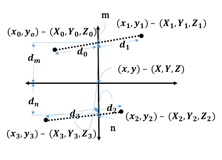
Figure 1: Bi-linear interpolation.

Figure 2 shows image taken from above a desk. The table is approximately 0.5 meters from the camera whereas the floor is approximately 1.3 meters from the camera.

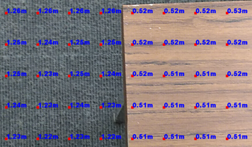
Figure 2: After alignment of depth information with RGB information, we see the difference between depth of table and depth of the floor from the camera – in an image taken from above the desk.

3.2 Size Estimation

Here we describe the different methods we use for object segmentation and size (object height) estimation.

Scheme 1: Depth based clustering
Our first scheme involves using depth information alone to cluster the pixels. This enables us to obtain a tight boundary for an object. Specifically, we cluster the pixels of the image into 3 clusters: background, foreground, and pixel with no depth information (typically filled in by 0s), using kmeans clustering from SciPy [14]. Depth of the pixels are used for computing the distance measure in the kmeans algorithm. We pick the second cluster as the foreground cluster. The object of interest is contained in the second cluster due to the ordering of depth information (pixels with no depth information are at depth 0, followed by foreground pixels, followed by background pixels which are the farthest).

In cases where there is only a single object to be measured in an image, this approach is very useful. Interestingly, this method can accurately estimate the dimensions of objects like the box shown in Figure 3 where color based differentiation is very challenging due to the white object on the white background.

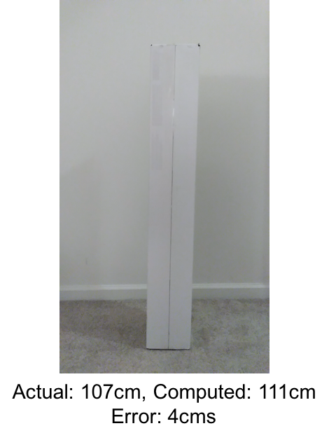
Figure 3: Depth based clustering can segment out objects in cases where RGB based segmentation is challenging.

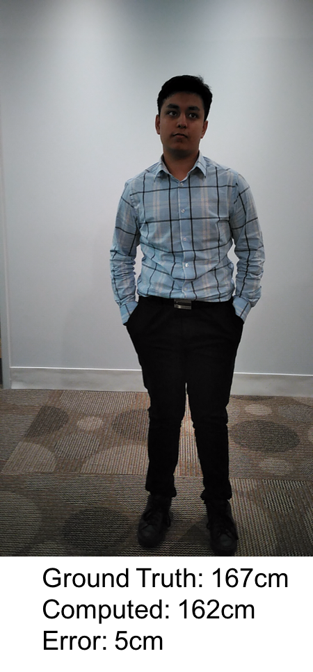
(a)

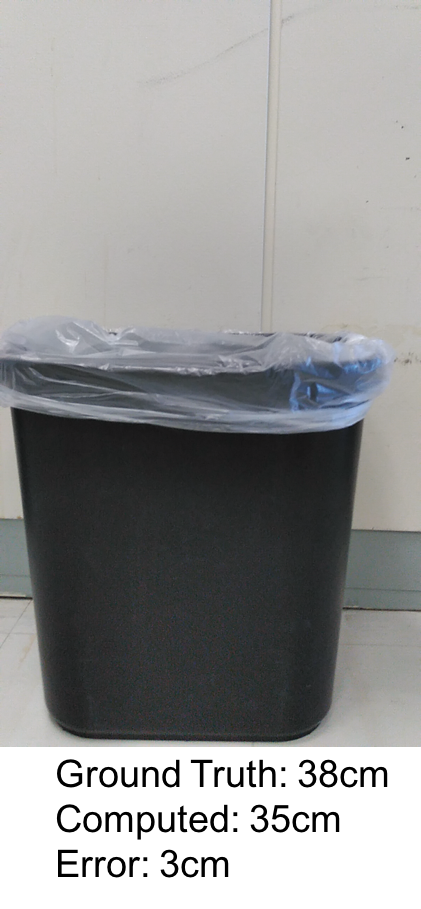
(b)

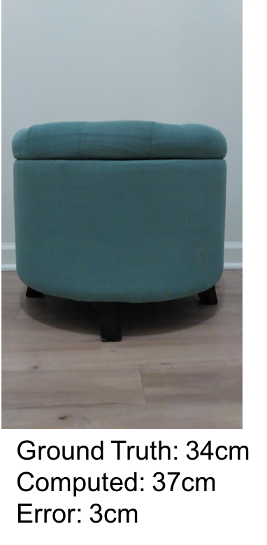
(c)

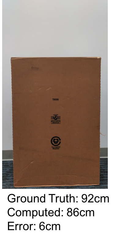
(d)

Figure 4: Size estimation results based on depth based clustering alone.

Figure 4 shows size estimation results on several other different subjects. Note that the results are very accurate in cases where a single subject is present. In cases where multiple objects are present in a cluttered scene, depth based clustering alone is not sufficient and thus we use object detection along with depth based clustering as described below.

Scheme 2: RGB object detection + depth based clustering
Since above explained depth based clustering alone is not sufficient when multiple objects are present in a scene, in this approach we first leverage off-the-shelf pre-trained CNNs to detect the objects of interest within the scene. We use off-the-shelf pre-trained CNNs so as to minimize the requirement of labelled data for re-training. We use object detection from [17] to obtain bounding boxes around objects of interest. This uses RGB information alone to obtain the bounding box. Different object detection algorithms can be used for RGB information based bounding box detection. The state-of-the-art schemes are based on Deep Convolutional Neural Networks. Once the bounding box is obtained as shown in Figure 5 (a), to isolate the object more tightly and segment it out, we cluster the pixels within the bounding box based on the depth information. An example clustered image is shown in Figure 5 (b). Once we have cleanly segmented out the object, we are able to measure the dimensions based on the $(X,Y,Z)$ information of the extreme points (pixels).

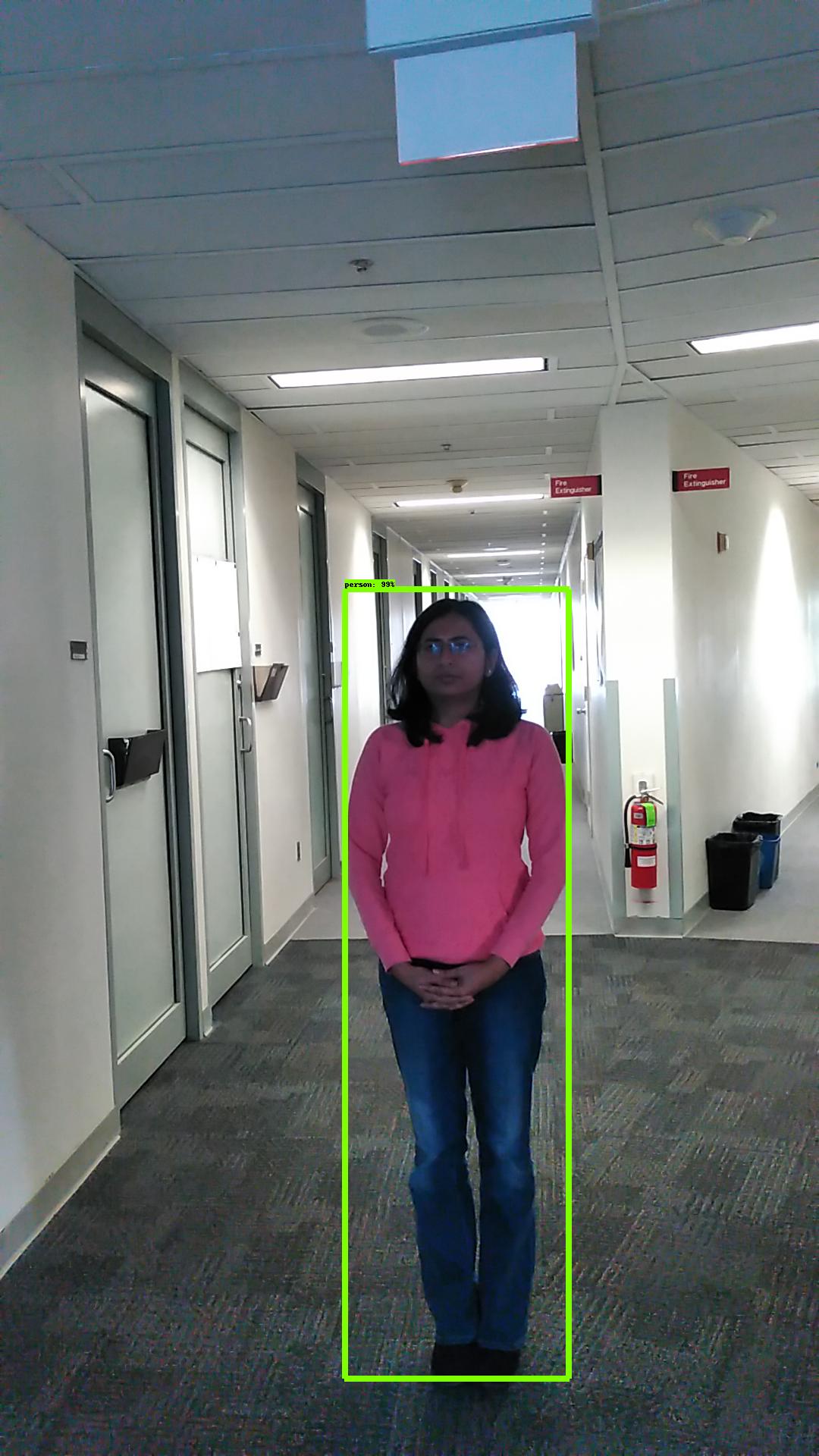
(a) Output after object detection.

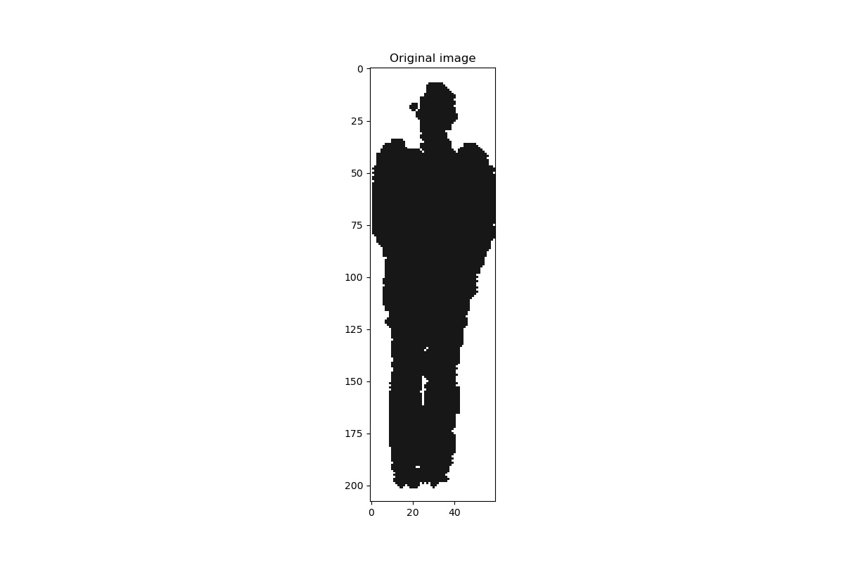
(b) Output after depth based clustering.

Figure 5: Intermediate results of object detection followed by depth based clustering.

Figure 6 shows size estimation results of object detection followed by depth based clustering on humans. The scheme works accurately without requiring that the person should stand against a clear background.

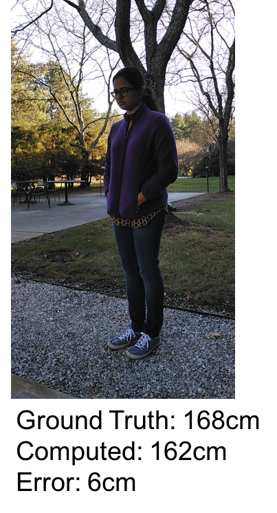
(a)

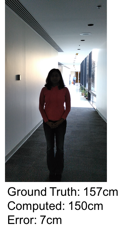
(b)

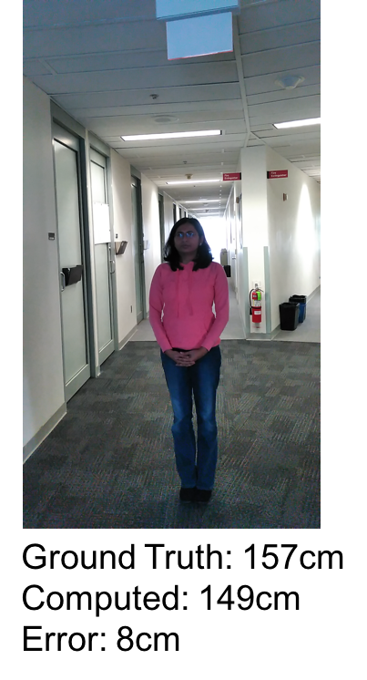
(c)

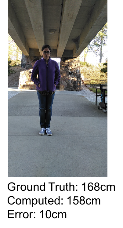
(d)

Figure 6: Size estimation results based on object detection + depth based clustering. Experiments were done both indoors and outdoors as seen in the images.

Scheme 3: Re-training YOLO for early fusion
This is our on-going work. To further improve the accuracy of object localization, CNN pipelines can be trained to fuse RGB features with depth based features. We choose YOLO pipeline due to its efficiency and real-time nature. We obtain HHA features as described in  [8]. HHA channels are then fused with RGB to create a 6 channel image. The early fusion minimizes the number of parameters in the CNN for high efficiency of computation. This improves the accuracy of localization because HHA features can help where RGB is not distinguishing or clear enough for object detection. This approach combines the benefits of the previous approaches, i.e., (i) depth information helps even in situations where color alone is not sufficient and (ii) this approach can be used in cluttered scenes with multiple objects. Once the object is accurately detected, the depth based clustering and object size estimation can be performed similar to above schemes.

4 Discussion and Conclusion

Object dimensions can be accurately estimated using color camera information along with point cloud information. In order to do so accurately, we require dense point cloud information of the object. In our experiments we found that point cloud information maybe missing in case of black or metallic objects. Stereo imagery can help in cases where such data sparsity is a problem. Further, the accuracy of size estimation is higher in cases where background is not in close proximity of the object – thus enabling accurate depth based segmentation.

5 Acknowledgement

Research was sponsored by the Army Research Laboratory and was accomplished under Cooperative Agreement Number W911NF-09-2-0053 (the ARL Network Science CTA). The views and conclusions contained in this document are those of the authors and should not be interpreted as representing the official policies, either expressed or implied, of the Army Research Laboratory or the U.S. Government. The U.S. Government is authorized to reproduce and distribute reprints for Government purposes notwithstanding any copyright notation here on.

References

- [1] X. Chen, K. Kundu, Z. Zhang, H. Ma, S. Fidler, and R. Urtasun. Monocular 3d object detection for autonomous driving. In IEEE CVPR, 2016.
- [2] X. Chen, K. Kundu, Y. Zhu, A. Berneshawi, H. Ma, S. Fidler, and R. Urtasun. 3d object proposals for accurate object class detection. In Proceedings of the 28th International Conference on Neural Information Processing Systems - Volume 1, NIPS’15, pages 424–432, Cambridge, MA, USA, 2015. MIT Press.
- [3] X. Chen, K. Kundu, Y. Zhu, H. Ma, S. Fidler, and R. Urtasun. 3d object proposals using stereo imagery for accurate object class detection. IEEE Transactions on Pattern Analysis and Machine Intelligence, PP(99):1–1, 2017.
- [4] X. Chen, H. Ma, J. Wan, B. Li, and T. Xia. Multi-view 3d object detection network for autonomous driving. CoRR, abs/1611.07759, 2016.
- [5] M. Engelcke, D. Rao, D. Z. Wang, C. H. Tong, and I. Posner. Vote3deep: Fast object detection in 3d point clouds using efficient convolutional neural networks. CoRR, abs/1609.06666, 2016.
- [6] R. B. Girshick. Fast R-CNN. CoRR, abs/1504.08083, 2015.
- [7] R. B. Girshick, J. Donahue, T. Darrell, and J. Malik. Rich feature hierarchies for accurate object detection and semantic segmentation. CoRR, abs/1311.2524, 2013.
- [8] S. Gupta, R. B. Girshick, P. Arbelaez, and J. Malik. Learning rich features from RGB-D images for object detection and segmentation. CoRR, abs/1407.5736, 2014.
- [9] K. Khoshelham and E. O. Elberink. Accuracy and resolution of kinect depth data for indoor mapping applications.
- [10] J. Kongsro. Estimation of pig weight using a microsoft kinect prototype imaging system. Comput. Electron. Agric., 109(C):32–35, Nov. 2014.
- [11] A. Mousavian, D. Anguelov, J. Flynn, and J. Kosecka. 3d bounding box estimation using deep learning and geometry. CoRR, abs/1612.00496, 2016.
- [12] J. Redmon, S. K. Divvala, R. B. Girshick, and A. Farhadi. You only look once: Unified, real-time object detection. CoRR, abs/1506.02640, 2015.
- [13] S. Ren, K. He, R. B. Girshick, and J. Sun. Faster R-CNN: towards real-time object detection with region proposal networks. CoRR, abs/1506.01497, 2015.
- [14] SciPy K-means. https://docs.scipy.org/doc/scipy/reference/cluster.vq.html.
- [15] E. Shelhamer, J. Long, and T. Darrell. Fully convolutional networks for semantic segmentation. IEEE Trans. Pattern Anal. Mach. Intell., 39(4), Apr. 2017.
- [16] Tango Transforms. https://developers.google.com/tango/apis/java/reference/TangoCameraIntrinsics.
- [17] Tensorflow Object Detection AP. https://github.com/tensorflow/models/tree/master/research/object_detection.
- [18] Velodyne LIDAR. http://velodynelidar.com/hdl-32e.html.
- [19] D. Z. Wang and I. Posner. Voting for voting in online point cloud object detection. In Proceedings of Robotics: Science and Systems, Rome, Italy, July 2015.