FUGIN: Molecular gas in a Spitzer bubble N4: possible evidence for a cloud–cloud collision as a trigger of massive star formations

Abstract

Herein, we present the ¹²CO ($J$=1–0) and ¹³CO ($J$=1–0) emission line observations via the FOREST Unbiased Galactic plane Imaging survey with the Nobeyama 45-m telescope (FUGIN) toward a Spitzer bubble N4. We observed clouds of three discrete velocities: 16, 19, and 25 km s^-1. Their masses were $0.1\times 10^{4}$ $M_{\odot}$, $0.3\times 10^{4}$ $M_{\odot}$, and $1.4\times 10^{4}$ $M_{\odot}$, respectively. The distribution of the 25-km s^-1 cloud likely traces the ring-like structure observed at mid-infrared wavelength. The 16- and 19-km s^-1 clouds have not been recognized in previous observations of molecular lines. We could not find clear expanding motion of the molecular gas in N4. On the contrary, we found a bridge feature and a complementary distribution, which are discussed as observational signatures of a cloud–cloud collision, between the 16- and 25-km s^-1 clouds. We proposed a possible scenario wherein the formation of a massive star in N4 was triggered by a collision between the two clouds. The time scale of collision is estimated to be 0.2–0.3 Myr, which is comparable to the estimated dynamical age of the Hii region of $\sim$0.4 Myr. In N4W, a star-forming clump located west of N4, we observed molecular outflows from young stellar objects and the observational signature of a cloud-cloud collision. Thus, we also proposed a possible scenario in which massive- or intermediate-mass star formation was triggered via a cloud–cloud collision in N4W.

1 Introduction

1.1 Massive star formation

Massive stars are important objects in the galactic environment due to their powerful influence on the interstellar medium via ultraviolet radiation, stellar winds, and supernova explosions. It is therefore of fundamental importance to understand the mechanisms of massive star formation, although these mechanisms still remain elusive (e.g., Zinnecker & Yorke (2007); Tan et al. (2014)).

Recently, supersonic cloud–cloud collision (CCC) has been discussed as an important triggering mechanism of massive star formation because of the large mass accretion associated with the compressed region between colliding two clouds. Observational studies have suggested the possible evidence of CCCs in Hii regions (with one or several young O-stars) and in super star clusters (with 10–20 O-stars) in the Milky Way and the Large Magellanic Cloud (Fukui et al. (2014, 2015, 2018a, 2018b, 2018c); Furukawa et al. (2009); Enokiya et al. (2018); Hayashi et al. (2018); Kohno et al. (2018); Nishimura et al. (2018, 2017); Ohama et al. (2010, 2018a, 2018b); Sano et al. (2017, 2018); Shimoikura et al. (2013); Torii et al. (2011, 2015, 2017a, 2017b, 2018); Tsuboi et al. (2015); Tsutsumi et al. (2017)). Magneto-hydrodynamical simulations of the formation of the massive clumps that may form massive stars in the collision-compressed layer have also been discussed (Inoue & Fukui (2013); Inoue et al. (2018)). Furthermore, comparisons between the observations and numerical calculations (Habe & Ohta (1992); Anathpindika (2010); Takahira et al. (2014, 2017)) have indicated two important observational signatures of CCCs: the “bridge feature” in position-velocity diagrams and the “complementary spatial distribution” in the sky between two colliding clouds, which provide useful diagnostics to identify CCCs using molecular line observations (Fukui et al. (2018a)). Bridge features are relatively weak CO emissions at intermediate velocities between two colliding clouds with different velocities. When a smaller cloud drives into a larger cloud, the smaller cloud caves the larger cloud owing to the momentum conservation (Haworth et al. (2015a)), and a dense compressed layer is formed at the collision interface, resulting in a thin, turbulent layer between the larger cloud and the compressed layer. If one observes a snapshot of this collision with a viewing angle parallel to the axis of collision, two separated velocity peaks connected by an intermediate–velocity emission with lower intensity feature could be observed in position-velocity diagrams.

1.2 Spitzer bubble N4

Churchwell et al. (2006, 2007) listed $\sim$600 objects with Spitzer 8 $\mu$m emission in a ring-like morphology on the Galactic plane ($l=10^{\circ}$–$65^{\circ}$ and $295^{\circ}$–$350^{\circ}$) and termed these objects as Spitzer bubbles. The 8 $\mu$m emission [from hot dust and polycyclic aromatic hydrocarbon (PAH) molecule] of Spitzer bubbles surrounds the radio continuum (from ionized gas) and the 24 $\mu$m emission (from warm dust). According to Elmegreen & Lada (1977), ultraviolet radiation from massive stars creates an expanding Hii region and the interstellar gas and dust can be collected in the circumference of the Hii region. As a result, dense ring- or shell-like gas/dust clouds are formed, which collapse to form stars. This is called as the “collect and collapse” process. This process has been suggested by some observational studies to operate in Spitzer bubbles (e.g., Deharveng et al. (2009, 2010); Zavagno et al. (2010)).

Figure 1(a) shows a composite color image of the Spitzer/MIPSGAL 24 $\mu$m (red) and Spitzer/GLIMPSE 8$\mu$m (green) emissions around N4 and N4W. N4 and N4W are located a little far from the middle of the Galactic plane, and seem to be relatively isolated objects from the surrounding Hii regions. Figure 1(b) shows a closeup figure of Figure 1(a). N4 has an almost complete ring-like structure in the 8 $\mu$m emission and the Hii region inside the ring. In previous studies, molecular clouds associated with N4 have been detected and the clouds show a ring-like structure (Li et al. (2013)), and their radial velocities ($V_{\rm LSR}$) are centered on $\sim$25 km s^-1. According to the parallax-based distance estimator (Reid et al. (2016)), this $V_{\rm LSR}$ and direction corresponds to a probable distance of 2.80 kpc$\pm$0.30 kpc, and hence, we adopted a distance of 2.8 kpc to N4. The radius of the ring is $\sim$2^′, which corresponds to $\sim$1.6 pc. The estimated total Lyman continuum [log($N_{\rm Lym}$ s^-1) = 48.18] indicates that a main O8.5–O9V star is responsible for the ionization of N4 (Liu et al. (2016)).

Watson et al. (2010) investigated the distribution of young stellar object (YSO) candidates around N4, and found that there does not appear to be an overdensity of YSOs along the shell. Therefore Watson et al. (2010) suggested that there is no evidence for the triggered star formation via the “collect and collapse” process, although they claimed that the triggered star formation could not be ruled out because YSO samples are not complete in this region. On the contrary, by observing the ¹²CO ($J$=1–0), ¹³CO ($J$=1–0), and C¹⁸O ($J$=1–0) emissions, Li et al. (2013) found an expanding motion of the molecular clouds associated with N4. They suggested that the formation of a massive star candidate (labeled as S2 in Li et al. (2013)) on the ring may be triggered by the expansion of the Hii region formed by a massive star candidate (labeled as S1 in Li et al. (2013)); however, the formation mechanism of S1, which is the star exciting N4 and located inside the ring, remains unclear in this scenario.

N4W, located $\sim 5^{\prime}$ west of N4, is a star-forming clump hosting YSOs and a submillimeter source (Chen et al. (2016)). Chen et al. (2016) identified four YSOs with at least intermediate mass in the innermost area by the observations of J, H, and Ks bands and found that these YSOs are almost coeval.

1.3 Paper overview

In this paper, we report an observational study of the Spitzer bubble N4 and N4W using the ¹²CO ($J$=1–0) and ¹³CO ($J$=1–0) dataset obtained via the FUGIN project (Minamidani et al. (2016); Umemoto et al. (2017)), whose spatial resolution is approximately 3 times higher than the previous CO observations, to investigate the formation process of N4 and N4W. Section 2 describes these datasets. In Section 3, we describe the large-scale CO distribution (Subsection 3.1), present the velocity structure of the molecular clouds (Subsection 3.2), compare the ¹²CO ($J$=1–0) emission with the ¹²CO ($J$=3–2) archive data obtained using the James Clerk Maxwell Telescope (JCMT; Subsection 3.3), and estimate the physical parameters of the molecular outflow associated with N4W (Subsection 3.4). In Section 4, we discuss massive star formation and the Hii region in N4 via a comparison with other massive-star forming regions, and the star formation in N4W.

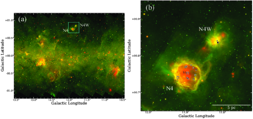
Figure 1: (a) A composite color image of the Spitzer/MIPSGAL 24 $\mu$m (red) and Spitzer/GLIMPSE 8$\mu$m (green) emissions. (b) Same as (a), but a closeup figure toward N4 and N4W. Square symbols represent the massive star candidates identified by Li et al. (2013). In particular, the larger square symbols represent S1 and S2. Crosses represent the YSOs identified by Chen et al. (2016).

2 Datasets

Observations of N4 were conducted as a part of the FUGIN project (Umemoto et al. (2017)) using the Nobeyama Radio Observatory (NRO) 45-m telescope. Details of the observations, calibration, and data reduction are summarized in Umemoto et al. (2017). In this study, we used the data of the ¹²CO ($J$=1–0) and ¹³CO ($J$=1–0) emissions covering $l=12\fdg 05$–$11\fdg 70$ and $b=0\fdg 65$–$1\fdg 00$ ($0\fdg 35\times 0\fdg 35$). The beam size of the NRO 45-m telescope is $\sim 15^{\prime\prime}$ at 115 GHz, and the effective angular resolution is $\sim 20^{\prime\prime}$ , which is due to the scanning pattern of the observations (Umemoto et al. (2017)). The Spectral Analysis Machine for the 45-m telescope (SAM45) spectrometer (Kuno et al. (2011)) was used with a frequency resolution of 244.14 kHz, and the effective velocity resolution was 1.3 km s^-1 at 115 GHz. The typical system noise temperatures ($T_{\rm sys}$), including atmosphere, were $\sim$150 K and $\sim$250 K at 110 and 115 GHz, respectively. $T_{\rm sys}$ at 115 GHz is higher than that of 110 GHz because of effects of atmosphere. The final cube data comprise spatial grids of $8.5^{\prime\prime}\times 8.5^{\prime\prime}$ and velocity channels of 0.65 km s^-1. The final root-mean-square noise temperature $T_{\rm{rms}}$ in $T_{\rm{mb}}$ scale are 1.5 K and 0.7 K per velocity channel for the ¹²CO ($J$=1–0) and ¹³CO ($J$=1–0), respectively, after the intensity calibration. Based on the observations of standard sources, the intensity variations were less than 10%–20% and 10% for ¹²CO ($J$=1–0) and ¹³CO ($J$=1–0), respectively.

We used the ¹²CO ($J$=3–2) archive data obtained with the Heterodyne Array Receiver Programme (HARP) installed on the JCMT. The observations covered a $0\fdg 15\times 0\fdg 15$ area, including N4, but not including N4W. The data have an angular resolution of 14^′′ and a velocity resolution of 0.44 km s^-1. At 345 GHz, the main beam efficiency for HARP is 0.64$\pm$0.10.

To improve the signal-to-noise ratio and compare the $J$=1–0 data with the $J$=3–2 data at the same angular resolution, we convolved the dataset using a Gaussian function to be FWHM 30^′′ for both the $J$=1–0 data data and the $J$=3–2 data. We also convolved the dataset for the velocity axis to be at a resolution of 1.3 km s^-1 using the same method.

3 Results

3.1 Large-scale CO distribution

Figure 2 shows the integrated intensity map of the ¹³CO ($J$=1–0) emission between the velocities of 12 and 37 km s^-1, which covers the entire velocity range of N4 and N4W. The distribution of CO gas is consistent with previous studies (Li et al. (2013)) with a resolution of $>52^{\prime\prime}$. The triangular symbols represent the YSOs identified by Liu et al. (2016) in N4. Most YSOs were distributed near the ring. Massive star candidates inside the ring were identified using near-infrared and mid-infrared data in N4 (Li et al. (2013)) and represented by square symbols. In N4, the molecular clouds seem to be distributed along the infrared 8 $\mu$m ring shown in Figure 1, suggesting an association between the distributions of molecular clouds and dust. Black crosses represent intermediate-mass YSOs (Chen et al. (2016)) in N4W. Molecular clouds in N4W are associated with the infrared emission (8 $\mu$m and 24 $\mu$m) and the YSOs.

The maximum column densities ($N({\rm H_{2}})$) were estimated to be $1.1\pm 0.2\times 10^{23}$ cm^-2 and $0.8\pm 0.1\times 10^{23}$ cm^-2 at 12 – 37 km s^-1 for N4 and N4W, respectively, which were derived from the ¹³CO ($J$=1–0) intensity and the local thermodynamic equilibrium (LTE) analysis. The estimated errors are due to mainly the calibration errors in the CO dataset (the same hereinafter). In this derivation, we assumed that the ¹²CO ($J$=1–0) emission lines are optically thick and that the excitation temperatures ($T_{\rm ex}$) were derived from the ¹²CO ($J$=1–0) peak brightness temperatures for each pixel (the derived $T_{\rm ex}$ is typically 10–40 K). We adopted an abundance ratio of [¹²CO]/[¹³CO]$=77$ (Wilson & Rood (1994)) and a fractional ¹²CO abundance of $X$(¹²CO) = [¹²CO]/[H₂]$=10^{-4}$ (Frerking et al. (1982); Leung et al. (1984)), and thus, $X$(¹³CO) = [¹³CO]/[H₂]$=1.3\times 10^{-6}$. Molecular masses were estimated to be $2.8\pm 0.4\times 10^{4}$ $M_{\odot}$ and $2.1\pm 0.3\times 10^{4}$ $M_{\odot}$ at 12 – 37 km s^-1 for N4 and N4W, respectively.

Figure 3 shows the large-scale velocity channel maps of the ¹²CO ($J$=1–0) emissions at a velocity step size of 2.6 km s^-1. We also present the velocity channel maps of the ¹³CO ($J$=1–0) emissions in Figure 16 in the appendix for supplements. The ¹²CO ($J$=1–0) emissions show extended gas distributions, whereas the ¹³CO ($J$=1–0) emissions show some clumpy structure. In the 22.2 – 24.8 km s^-1 panel, molecular ring-like structures were seen not only in N4 but also in N4W. In addition to the 22.2 – 27.4 km s^-1 panel, relatively diffuse components were observed in the 14.4 – 17.0 km s^-1, 17.0 – 22.2 km s^-1, and 27.4 – 30.0 km s^-1 panels.

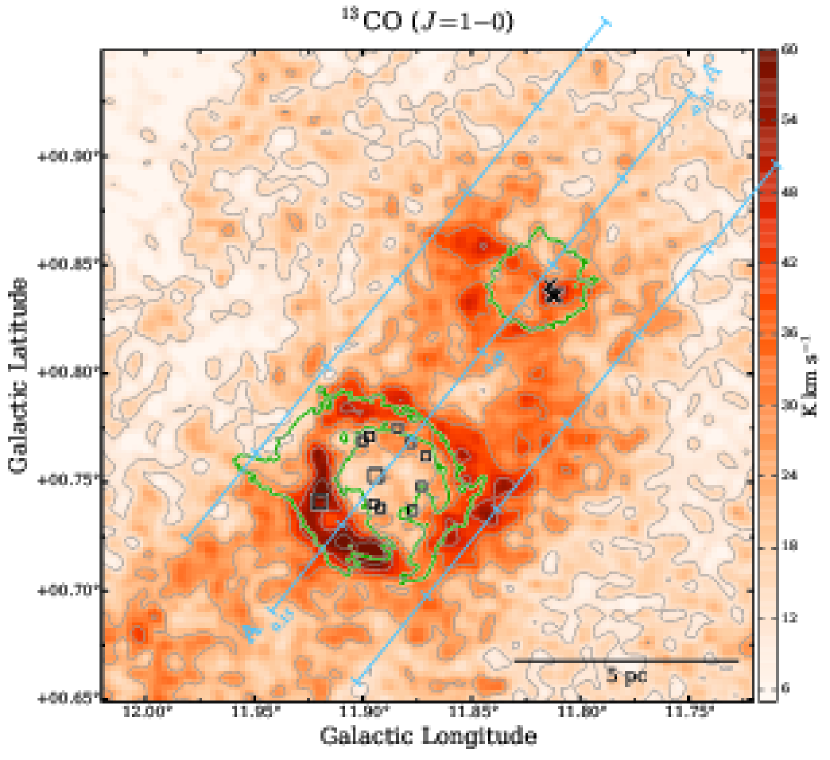
Figure 2: Integrated intensity map of the ¹³CO ($J$=1–0) emission between the velocities of 12 and 37 km s^-1. Black contours are plotted at every 12 K km s^-1 from 12 K km s^-1 ($\sim 5\sigma$). Green contours indicate the Spitzer/GLIMPSE 8$\mu$m intensity at 100  MJy str^-1. Blue lines indicate the direction and the width of the $p$–$v$ diagram shown in Figure 4. Square symbols represent the massive star candidates identified by Li et al. (2013).

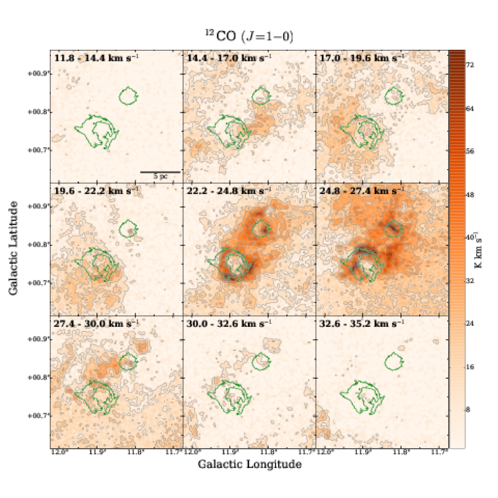
Figure 3: The velocity channel maps of the ¹²CO ($J$=1–0) emissions. Integration range of each panel is presented in the top-left corner of the panel. Black contours are drawn at every 8.5 K km s^-1 from 8.5 K km s^-1 ($\sim 5\sigma$). Square symbols represent the massive star candidates identified by Li et al. (2013). Green contours indicate the Spitzer/GLIMPSE 8$\mu$m intensity at 100 MJy str^-1.

3.2 Velocity structure of the molecular clouds

Figure 4 shows the position-velocity ($p$–$v$) diagram for the ¹²CO ($J$=1–0) emissions along the blue line in Figure 2 with a width of 6^′. In Figures 3 and 4, we identified three discrete intensity peaks with velocities of $\sim$16, 19, and 25 km s^-1 (hereinafter termed as “the 16-km s^-1 cloud”, “the 19-km s^-1 cloud”, and “the 25-km s^-1 cloud”, respectively). In Figure 3, these three components are shown in the 14.4–17.0, 17.0–22.2, and 22.2–27.4  km s^-1 panels, respectively. The 16-km s^-1 cloud and the 19-km s^-1 cloud have not been recognized in previous observations of molecular lines. Furthermore, we found that the 16-km s^-1 cloud and the 25-km s^-1 cloud are connected significantly ($>5\,\sigma$) at an OFFSET value of $\sim 0\fdg 05$ and an OFFSET value of $\sim-0\fdg 05$ in Figure 4. These clouds are therefore probably interacting with each other. In addition, a diffuse component with a velocity of $\sim$ 29 km s^-1 (i.e., the 29-km s^-1 cloud) can be observed in Figure 3 and Figure 16 in Appendix, although this component is blended with the 25-km s^-1 cloud in the $p$–$v$ diagram.

Figure 5(a) shows the ¹²CO ($J$=1–0) integrated intensity of the 16-km s^-1 cloud with an integrated velocity range from 14.4 to 17.0 km s^-1. The size of the 16-km s^-1 cloud is $\sim$5 pc $\times$3 pc. The left end of the cloud in the map is overlapped with the center of the infrared 8 $\mu$m ring, where the massive star candidates are identified. The mass and maximum column density ($N({\rm H_{2}})$) of the 16-km s^-1 cloud are estimated to be $0.12\pm 0.02\times 10^{4}$ $M_{\odot}$ and $0.7\pm 0.1\times 10^{22}$ cm^-2, respectively.

Figure 5(b) shows the ¹²CO ($J$=1–0) integrated intensity of the 19-km s^-1 cloud with an integrated velocity range from 17.7 to 20.2 km s^-1. This cloud extends around the infrared 8 $\mu$m ring, and the size of the cloud is approximately 8 pc $\times$8 pc. The mass and maximum $N({\rm H_{2}})$ of the 19-km s^-1 cloud are estimated to be $0.43\pm 0.06\times 10^{4}$ $M_{\odot}$ and $0.8\pm 0.1\times 10^{22}$ cm^-2, respectively.

Figure 5(c) shows the ¹²CO ($J$=1–0) integrated intensity of the 25-km s^-1 cloud within an integrated velocity range between 22.2 and 27.4 km s^-1. This cloud also has a distribution to likely trace the ring structure in N4. The mass and maximum $N({\rm H_{2}})$ of the 25-km s^-1 cloud are estimated to be $3.8\pm 0.6\times 10^{4}$ $M_{\odot}$ and $1.0\pm 0.2\times 10^{23}$ cm^-2, respectively.

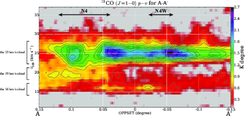
Figure 4: Position–Velocity ($p-v$) diagram of the ¹²CO ($J$=1–0) emissions along the blue line shown in Figure 2 from A to A^′ with an integrated width of 6^′ (between the upper and lower blue lines). Contours are plotted at every 0.1 K degree from 0.1 K degree ($\sim 5\sigma$). The black arrows indicate the area Spitzer/GLIMPSE 8μm intensity at $>$ $\sim$ 100 M Jy str^-1 shown in Figure 2.

3.3 ¹²CO ($J$=3–2)/($J$=1–0) intensity ratio

The color scale in Figures 5(d)–5(f) shows the integrated intensity ratio ¹²CO ($J$=3–2)/¹²CO ($J$=1–0) (hereinafter denoted by $R^{12}_{3210}$) of the 16-km s^-1 cloud, the 19-km s^-1 cloud, and the 25-km s^-1 cloud, respectively. The intensity ratio between two different rotational transitions reflects the kinematic temperature and/or the density of the gas. In Figure 5, $R^{12}_{3210}$ is relatively high ($>$0.7) at the ring structure of the 25-km s^-1 cloud, probably suggesting that the gas has been heated due to radiation from massive stars within the ring and/or the volume density of the gas is high. On the contrary, $R^{12}_{3210}$ of the 16-km s^-1 cloud and the 19-km s^-1 cloud were lower than that of the 25-km s^-1 cloud, typically $\sim$0.45 and $\sim$0.30, respectively.

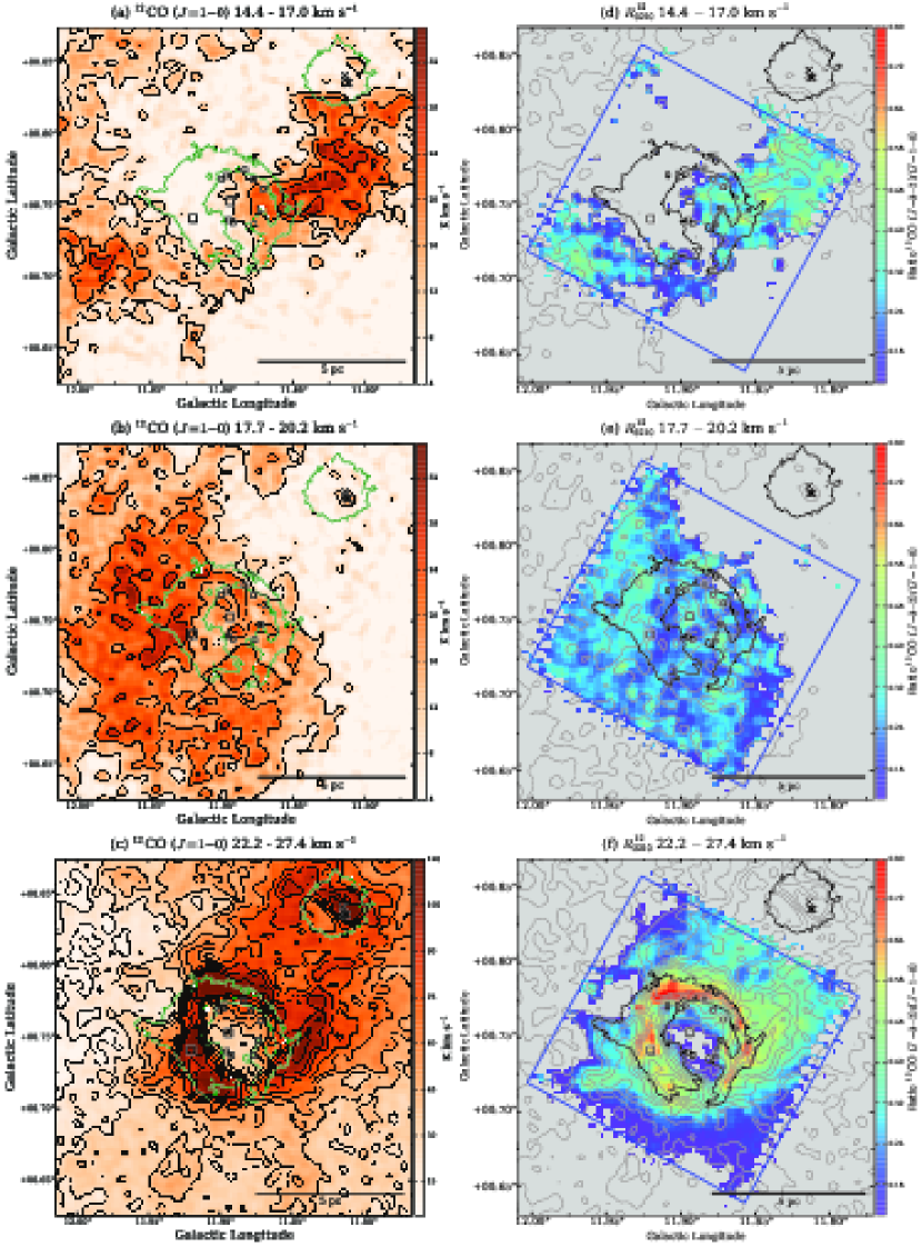
Figure 5: (a)–(c) Integrated intensity of the ¹²CO ($J$=1–0) of the 16-, 19-, and 25-km s^-1 clouds, respectively. Green contours indicate the Spitzer/GLIMPSE 8$\mu$m intensity at 100 MJy str^-1. (d)–(f) Integrated intensity ratio ¹²CO ($J$=3–2)/¹²CO ($J$=1–0) ($R^{12}_{3210}$) map of the 16-, 19-, and 25-km s^-1 clouds, respectively. Thin black contours indicate the ¹²CO ($J$=1–0) integrated intensity, and plotted every 8 K degree ($\sim 5\sigma$) from 10 K degree, every 8 K degree ($\sim 5\sigma$) from 10 K degree, and every 12 K degree ($\sim 5\sigma$) from 12 K degree, respectively. Blue large square indicates the area of the ¹²CO ($J$=3–2) data. Square symbols represent the massive star candidates identified by Li et al. (2013).

3.4 Molecular outflow in N4W

Figure 6 shows the velocity channel map of the ¹²CO ($J$=1–0) emission around N4W. A compact component with a large line width can be observed at $(l,b)=(11\fdg 812,0\fdg 837)$ with the velocity center at $\sim$25 km s^-1. In this position, four intermediate-mass YSOs, indicated by crosses, and their outflows have been identified by a previous study (Chen et al. (2016)). The compact component with a broad line width located on the YSOs is considered to be a molecular outflow from one of the YSOs. Figure 7 shows the distribution of the molecular outflow in two velocity ranges. The peak positions of the blue shifted and red shifted outflow lobes are slightly shifted from each other, although the separation is smaller than the resolution of the CO data.

We derived the physical parameters of this molecular outflow, e.g., mass ($M_{\rm flow}$), kinetic energy ($E_{\rm flow}$), momentum ($P_{\rm flow}$), dynamical timescale ($t_{\rm dyn}$), and mechanical luminosity ($L_{\rm m}$), by employing the method of Torii et al. (2017c), which assumes the LTE condition. Because the CO spectra of the outflow are blended with respect to the molecular clump of the 25-km s^-1 cloud, we first determined the velocity range of the CO spectra of the clump at the outflow position. The spatial extension of the clump was identified by drawing a contour onto the ¹³CO ($J$=1–0) integrated intensity map (integrated from 12 km s^-1 to 37 km s^-1) at the two-third level of the peak intensity delineated by circle A in Figures 6 and 7. Figure 8 show the averaged CO spectra in the circle A. A fit with a Gaussian function was performed for the ¹²CO ($J$=1–0) spectrum averaged over circle A, which provided a systemic velocity of 25 km s^-1 and a velocity width of 4.0 km s^-1. We estimated the mass of the molecular clump, which is possibly host the YSOs, of $4.1\pm 0.6\times 10^{2}\,M_{\odot}$ in the velocity range 22.2 – 27.4 km s^-1. This value is consistent with the estimation of Chen et al. (2016). We regard the residuals of the CO spectra and the Gaussian function as the molecular outflow components in the CO spectra (Figure 8). Since other components are blended in the spectra in the lower velocity side of the outflow, we derived the physical parameters only the higher velocity side of the outflow. Although the 29 km s^-1 component is blended into the higher velocity side with the outflow component, we ignore the 29 km s^-1 component because its intensity is low. Assuming that the inclination of the line-of-sight direction is 0^∘ or 45^∘, we estimated $M_{\rm flow}=\sum_{i}M_{{\rm flow,}i}=0.5\pm 0.1\times 10^{2}\,M_{\odot}$, total $P_{\rm flow}=\sum_{i}M_{{\rm flow,}i}v_{i}=249\pm 75\,M_{\odot}$ km s^-1 for 0^∘ and $352\pm 53\,M_{\odot}$ km s^-1 for 45^∘, and total $E_{\rm flow}=\sum_{i}M_{{\rm flow,}i}v_{i}^{2}=0.9\pm 0.1\times 10^{46}$ erg for 0^∘ and $1.8\pm 0.3\times 10^{46}$ erg for 45^∘, where $i$ refers to velocity channels. According to a statistical study of YSOs in our Galaxy by Wu et al. (2004), the estimated $M_{\rm flow}$ is approximately the intermediate value between the low mass group and the high mass group in the study, if we assume that the outflow stems from a single YSO.

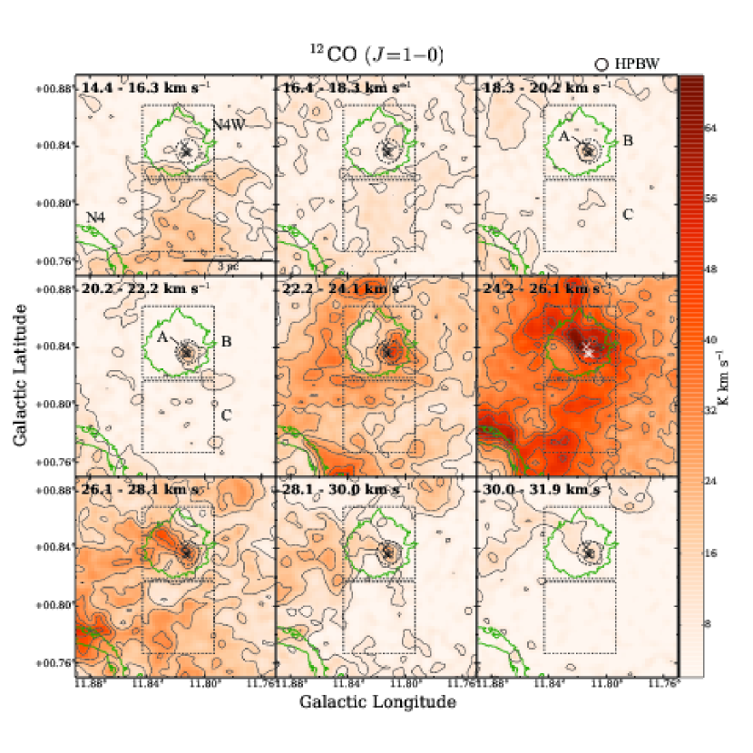
Figure 6: Velocity channel maps of the ¹²CO ($J$=1–0) emissions toward N4W. Integration range of each panel is presented in the top-left corner of the panel. Crosses represent the YSO candidates identified by Chen et al. (2016). Black contours are plotted at every 7.5 K km s^-1 from 7.5 K km s^-1 ($\sim 5\sigma$). Green contours indicate the Spitzer/GLIMPSE 8$\mu$m intensity at 100 MJy str^-1. Dotted circle A shows the area we used in Figure 8. Dotted squares B and C show the area we used in Figure 13.

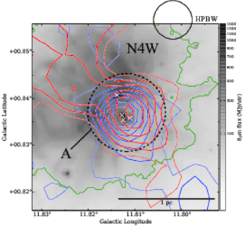
Figure 7: Gray scale shows the intensity of the Spitzer/GLIMPSE 8$\mu$m (green) emissions toward N4W, and the green contours indicate 100 MJy str^-1. Blue and red contours show the integrated intensity of the ¹²CO ($J$=1–0) emissions with the velocity range of 18.3 – 22.2 km s^-1 and 28.7 – 32.6 km s^-1, respectively. The contours are plotted at every 5 K km s^-1 from 10 K km s^-1 ($\sim 5\sigma$). Crosses represent the YSO candidates identified by Chen et al. (2016).

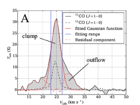
Figure 8: The averaged spectra in the circle A in Figure 6.

4 Discussion

4.1 Expanding motion of the molecular gas in N4

Li et al. (2013) observed N4 with ¹²CO ($J$=1–0), ¹³CO ($J$=1–0), and C¹⁸O ($J$=1–0) and speculated that N4 is more likely an inclined expanding ring than a spherical-bubble, although they also noted that observations with higher resolution are necessary to confirm this speculation. Li et al. (2013) also speculated that the formation of S2 on the ring was triggered by the compression due to the expanding motion of the ring. On the contrary, Chen et al. (2017) observed a magnetic field derived from near-IR polarization of reddened diskless stars located behind N4. They found that the direction of the magnetic field is curved and parallel to the ring and suggested that the star formation on the ring triggered by expanding motions might not easily occur because the estimated magnetic field is strong enough ($\sim$120 $\mu$G).

We investigate the detailed velocity structure of the 25-km s^-1 cloud by using our approximately 3 times high-angular resolution CO dataset. Figure 9(a) shows the ¹³CO ($J$=1–0) integrated intensity between the velocities of 12 and 37 km s^-1. Figures 9(b) and 9(c) show the $v$–$b$ diagram and $l$–$v$ diagram of the ¹³CO ($J$=1–0) emission, respectively, integrated between the blue dotted-lines in Figure 9(a). The lowest contour indicates $\sim 5\sigma$ level. If the molecular gas in N4 has an expanding spherical-bubble structure, elliptical shapes should be observed in Figures 9(b) and 9(c) as suggested by Figure 5 in Arce et al. (2011), which is a model of an expanding spherical-bubble inside a turbulent medium. However, we can not observe clear ellipse in Figures 9(b) and 9(c), which is consistent with the result of Li et al. (2013).

On the other hand, Figure 9(d) shows the $p$–$v$ diagram of the ¹³CO ($J$=1–0) emission along the ring with a width of 1^′ (between the black circles in Figure 9(a)). The lowest contour indicates $\sim 5\sigma$ level. If the molecular gas in N4 has an expanding ring structure as proposed by Li et al. (2013), Figure 9(d) should show a sinusoidal wave with a length of 2$\,\pi$ radian (one cycle) unless the expanding motion is perpendicular to the line-of-sight. However, we can not find a clear sinusoidal wave of the 25-km s^-1 cloud in Figure 9(d), though some velocity gradients are observed. For these reasons, we concluded that the molecular gas in N4 may not be expanding.

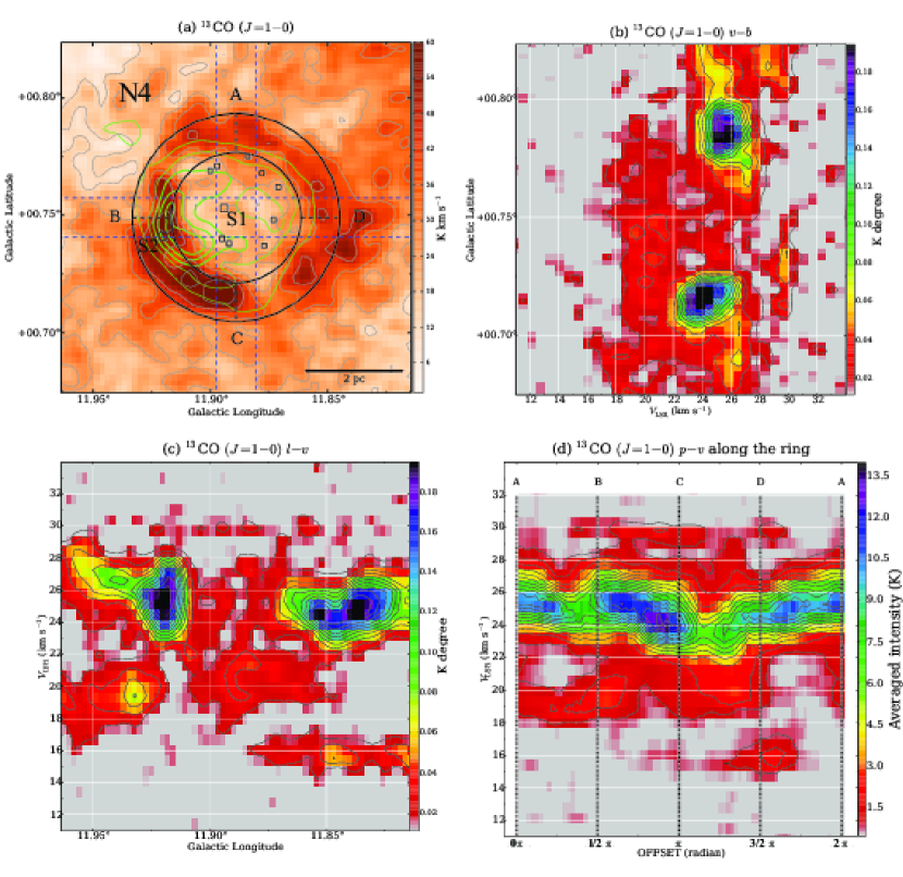
Figure 9: (a) The ¹³CO ($J$=1–0) integrated intensity between the velocities of 12 and 37 km s^-1. The green contours show the intensity of 20-cm radio continuum taken from the Multi-Array Galactic Plane Imaging Survey (MAGPIS, Helfand et al. (2006)) archive, and are plotted by 0.75 ($\sim 5\sigma$), 1.95, 3.15, 4.35, and 5.55 mJy Beam^-1. Square symbols represent the massive star candidates identified by Li et al. (2013). (b) The $v$–$b$ diagram of the ¹³CO ($J$=1–0) emission integrated between the vertical blue dotted-lines in Figure 9(a). Contours are plotted at every 0.018 K degree from 0.018 K degree ($\sim 5\sigma$). (c) The $l$–$v$ diagram of the ¹³CO ($J$=1–0) emission integrated between the horizontal blue dotted-lines in Figure 9(a). Contours are plotted at every 0.018 K degree from 0.018 K degree ($\sim 5\sigma$). (d) The $p$–$v$ diagram of the ¹³CO ($J$=1–0) emission along the ring with a width of 1^′ indicated by the black circles in Figure 9(a). Contours are plotted at every 1.0 K from 1.0 K ($\sim 5\sigma$).

4.2 Cloud–cloud collisions in N4 and N4W as an alternative scenario

4.2.1 N4

As shown in Figures 3, 5(c), and 5(f), the 25-km s^-1 cloud is clearly associated with N4. The 16-km s^-1 cloud is also possibly associated with N4 because it has slightly elevated $R^{12}_{3210}$, as shown in Figure 5(d). Meanwhile, it is not certain whether the 19-km s^-1 cloud is interacting with the 16-km s^-1 cloud and the 25-km s^-1 cloud. $R^{12}_{3210}$ of the 19-km s^-1 cloud is lower than those of the 16-km s^-1 cloud and the 25-km s^-1 cloud, and hence, it seems that the 19-km s^-1 cloud is not interacting with the Hii region. The location of N4 is the inner Galaxy, $l=11\fdg 8$, where heavy contamination is expected in these velocities. Therefore, the 19-km s^-1 cloud is possibly not directly interacting with N4, but it is overlapping with other clouds at the line-of-sight.

Herein, we found that the 16-km s^-1 cloud and the 25-km s^-1 cloud are connected in the $p$–$v$ diagram (Figure 4) toward N4. This is a bridge feature, which is discussed as a possible observational signature of CCC by previous studies (e.g., Haworth et al. (2015a, b)). Figure 10(a) shows an integrated intensity map of the ¹²CO ($J$=1–0) emissions of the 25-km s^-1 cloud (color scale) and the 16-km s^-1 cloud (blue contours). The Galactic east end of the 16-km s^-1 cloud in the map is located at the center of the ring structure of the 25-km s^-1 cloud, where the massive star candidates have been identified. Figure 10(b) shows an integrated intensity map of the ¹³CO ($J$=1–0) emissions. At the Galactic west side of the 25-km s^-1 cloud in the map, the two clouds show spatially complementary distributions, which is also discussed as a possible observational signature of CCC (Fukui et al. (2018a)).

Figure 11(a) shows the $p$–$v$ diagram between B and B^′ in Figure 10(a) through the 16-km s^-1 cloud and the 25-km s^-1 cloud. A bridge feature connecting the 16-km s^-1 cloud and the 25-km s^-1 cloud can be observed, and it further shows a V-shaped structure (black dashed lines). Such V-shaped structures in $p$–$v$ diagrams have been observed in other CCC objects (e.g., Fukui et al. (2018a); Ohama et al. (2018b)). We can also observe the 19-km s^-1 cloud in the $p$–$v$ diagram, but this can be determined to be distinct from the bridge feature.

We here test dynamical binding of the 16- and 25-km s^-1 clouds. If we tentatively assume that the two clouds are separated by 6 pc (same as lengths of the 16- and 25-km s^-1 clouds in N4) in space and by $9\,\times\,\sqrt{2}$ km s^-1 in velocity (we also assume the viewing angle of the relative motion between the two clouds as 45^∘ to the line-of-sight), the total mass required to gravitationally bind these two clouds can be calculated as $M=\frac{rv^{2}}{2G}=1.1\,\times 10^{5}M_{\odot}$. This is larger than the total molecular mass of N4 ($2.8\,\times 10^{4}M_{\odot}$) estimated in Section 3.1, indicating that the co-existence of the two velocity clouds in N4 can not be interpreted as the gravitationally bound system.

For these reasons, we proposed a CCC between the 16-km s^-1 cloud and the 25-km s^-1 cloud in N4. After the collision, a cavity was created in the molecular clouds, which permitted the formation of one or more massive stars at the compressed layer. At present, gas near the collision interface of the 16-km s^-1 cloud is broken up and ionized via UV radiation from the massive star(s).

The timescale of the collision (between the time when collision occurred and the present time) in N4 can be approximated estimated from the size of the cavity and the relative velocity between the two clouds. The size of the cavity in the $l$–$b$ plane is $\sim$3 pc. If we assume that the relative velocity parallel to the $l$–$b$ plane is same as the relative radial velocity and that the cavity is spherical, the estimated timescale of the collision is $3\,$pc$/9\,$km s${}^{-1}=0.2$–$0.3$ Myrs.

The red and blue triangles in Figure 10(a) represent Class I YSOs and Class II YSOs, respectively, and the uncolored triangles represents transitional disk YSOs (Liu et al. (2016)). Class I and Class II YSOs are located at the extension line of the 16-km s^-1 cloud elongation and at the left edge of the 16-km s^-1 cloud in the map. The formation of these YSOs is most likely triggered by the collision of the 16-km s^-1 cloud and the 25-km s^-1 cloud, although the formation of the other YSOs in N4 could not has been triggered because the age of the transitional disk YSOs is generally greater than 1 Myr (Currie & Sicilia-Aguilar (2011)).

4.2.2 N4W

As seen in Figures 3, and 5(c) the 25-km s^-1 cloud is associated not only with N4 but also with N4W. Figure 12 shows the $v$–$b$ diagram of the ¹²CO ($J$=1–0) emission from C to C^′ in Figure 10(a). We can see a diffuse component between the 16-km s^-1 cloud and the 25-km s^-1 cloud at a $b$ value of $\sim 0\fdg 80$ with the intensity of the ¹²CO ($J$=1–0) emission of $>5\sigma$. Figure 13 shows the average spectra within the squares B and C in Figure 6. Although the high-velocity wing emission of the molecular outflows from the YSOs is confined to within the area of square B, a faint emission connecting the 16-km s^-1 cloud and the 25-km s^-1 cloud can be detected within the area of square C.

For these reasons, the diffuse component between the two clouds may be a bridge feature similar to that observed in N4. In other words, even in N4W, a similar scenario of massive star formation triggered by the collision of the 16-km s^-1 and the 25-km s^-1 clouds is conceivable. Because the estimated $t_{\rm dyn}$ of the outflow from the YSOs is $<$ 0.1 Myr (Subsection 3.4) and Hii regions in N4W have not grown compared to those of N4, the molecular clouds in N4W were collided probably after the collision in N4 in this scenario. Chen et al. (2016) suggested the possibility that the four YSOs in N4W are coeval. The CCC scenario in N4W could explain the small age range of the reported YSOs since CCC can trigger star formation over a short time scale. We speculate that the non-uniform cloud morphology and density caused massive star formations in two places (N4 and N4W) despite the single pair of collisions.

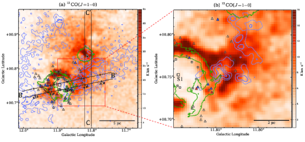
Figure 10: (a) Integrated intensity map of the ¹²CO ($J$=1–0) emission with a velocity range from 24.8 to 26.1 km s^-1 (color scale) (the 25-km s^-1 cloud) and from 15.1 to 16.4 km s^-1 (blue contours) (the 16-km s^-1 cloud). Contours are plotted every 6 K km s^-1 from 6 K km s^-1 ($\sim 5\sigma$). Square symbols represent the massive star candidates identified by Li et al. (2013). Triangle symbols represent the YSOs identified by Liu et al. (2016), and red, blue, and non-colored indicate Class I, Class II, and transitional disk, respectively. Green contours show the Spitzer/GLIMPSE 8$\mu$m intensity at 100 MJy str^-1 (b) Same as (a) but for the ¹³CO ($J$=1–0) emission at the red square region in (a). Contours are plotted every 1 K km s^-1 from 3 K km s^-1 ($\sim 5\sigma$).

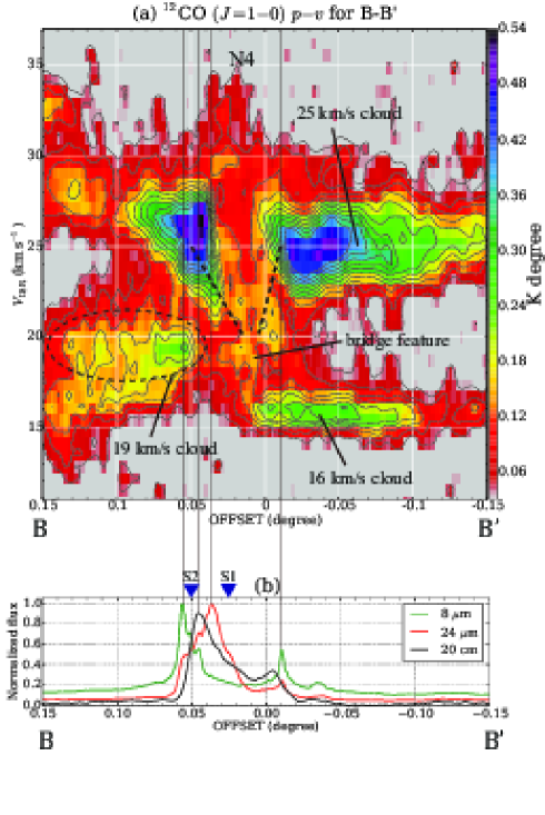
Figure 11: (a) $p-v$ diagram of the ¹²CO ($J$=1–0) along black axis in Figure 10(a) from B to B^′. Contours are drawn at every 0.08 K degree from 0.08 K degree ($\sim 10\sigma$). (b) Median intensity (perpendicular to the B–B^′ line) of the Spitzer/MIPSGAL 24 $\mu$m (red) and Spitzer/GLIMPSE 8$\mu$m (green) along the B–B^′ line in (a) with a width of 1.2^′.

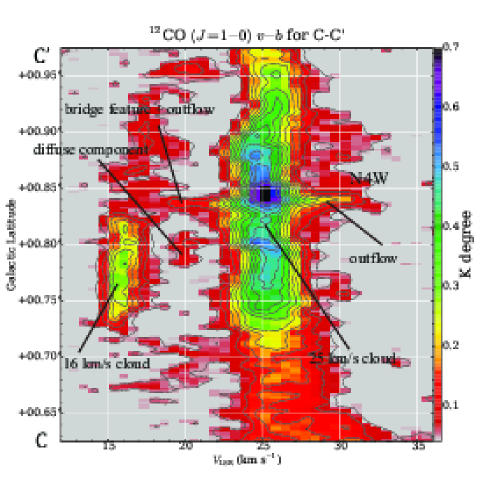
Figure 12: $v-b$ diagram of the ¹²CO ($J$=1–0) from C to C^′ in Figure 10(a). Contours are plotted at every 0.05 K degree from 0.05 K degree ($\sim 5\sigma$).

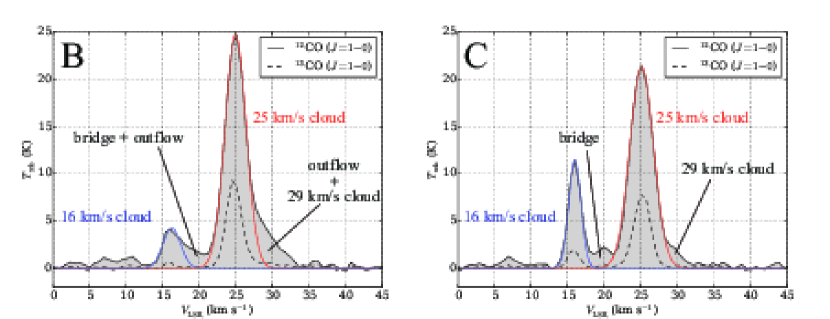
Figure 13: Averaged spectra of ¹²CO ($J$=1–0) emission (solid line) and ¹²CO ($J$=1–0) emission (broken line) in the squares B (left) and C (right) in Figure 6, respectively.

4.3 Ages of the Hii region in N4

One can calculate a dynamical age of the Hii region using the analytical model of the D-type expansion developed by Spitzer (1978). The Lyman continuum photon flux of N4 was estimated to be $log(N_{\rm ly}\,{\rm s^{-1}})=48.18$ (Liu et al. (2016)). The initial volume density of the gas was estimated to be approximately 4$\times$10³ cm^-3 when assuming a uniform spherical distribution with a radius of 4 pc with a total molecular mass of $\sim 2.8\times$10⁴ M_⊙. In addition, we assumed an electron temperature of 8000 K. Given these parameters, the age of the Hii region with a radius of 1.5 pc is estimated to be $\sim$0.4 Myr. This is almost consistent with the age of the time scale of the CCC estimated above 0.2–0.3 Myr, which supports the CCC scenario that explains the formation of the massive star(s).

4.4 Massive stars in N4 and N4W

Figure 14 shows a closeup of Figure 1, where the blue contours indicate the intensity of the 20-cm radio continuum taken from the Multi-Array Galactic Plane Imaging Survey (MAGPIS, Helfand et al. (2006)) archive. As mentioned above, Li et al. (2013) suggested that the most massive and luminous star in N4 is S1, which is located at the center of the ring, and that the formation of star S2, located on the ring, was triggered by the expansion of the Hii region. However, the brightest massive stars in the Spitzer bubbles are not necessarily located at the center (e.g., Torii et al. (2015); Ohama et al. (2018a)). In N4, Li et al. (2013) showed that the brightest massive star candidate in the $J$ band and the $J-H$ is S2. Figure 11(b) shows a plot of the median intensity (with the direction perpendicular to the B–B^′) of Spitzer/MIPSGAL 24 $\mu$m (red) and Spitzer/GLIMPSE 8$\mu$m (green) along the B–B^′ line in Figure 10(a) with a width of 1.2^′. Of all massive star candidates reported by Li et al. (2013), the closest to the peak of the 20-cm radio continuum emission, which traces Hii regions, is S2, as observed in Figures 11(b) and 14. For these reasons, we speculate that the most massive and luminous star in N4 is most likely S2, although we can not rule out the possibility that S1 was most influential on the IR bubble morphology. Follow-up near-IR and optical observations would reveal the position and spectral type of the massive star(s) in N4.

On the contrary, in N4W, no massive star candidates were identified, although Chen et al. (2016) identified one Class I and three Class II YSOs in the innermost area from observations of the $J$, $H$, and $Ks$ bands. For these YSOs, the authors derived the crude lower limits of their $L_{\rm bol}$ to be $1$–$2\,\times 10^{2}\,L_{\odot}$, suggesting at least intermediate masses for the YSOs. Using AKARI far-IR data (60, 90, and 140 $\mu$m) (Kawada et al. (2007)), we estimated the far-IR total luminosity of N4 and N4W by employing the method of Solarz et al. (2016). As a result, $7.9\,\times 10^{4}\,L_{\odot}$ and $3.7\,\times 10^{4}\,L_{\odot}$ were derived for N4 and N4W, respectively. Since these values correspond to approximately a single O8V star and a single O9.5V star, respectively (Martins et al. (2005)), there might be an embedded massive star in N4W, which has not yet been identified.

Figure 15 shows a summary of the assumed CCC scenario discussed in Subsection 4.2, which considers the location of the massive star in N4 and the YSOs in N4W. Figure 15(a) shows a schematic view from the Galactic east at the time the collision started (a few $10^{5}$–$10^{6}$ years ago) and when the molecular clouds in N4 began to be compressed. As a result, the 16-km s^-1 cloud created a cavity (the ring-like structure) in the 25-km s^-1 cloud as demonstrated by the numerical simulation of CCC (see Figure 6 in Takahira et al. (2014)). Thereafter the massive star S2 was formed in the compressed layer according to the model proposed in a study of Habe & Ohta (1992). Figure 15(b) shows a schematic view from the Galactic east at the present time. S2 has either ionized or broken up the surrounding neutral materials. The ionized gas fills up the cavity and erodes the inner surface of the cavity, which is the ring structure observed at 8 $\mu$m. This CCC scenario is able to explain the formation of both the massive star and the ring in N4. In addition, the molecular clouds in N4W began to be compressed and YSOs were formed. Note that, the curve of the 16-km s^-1 cloud in this sketched diagrams Figure 15(a) and 15(b) is one instance to explain the star formation history in both N4 and N4W. Figures 15(c1) and 15(c2) show schematic views of the sky plane and integrated intensity map of the CO gas, respectively.

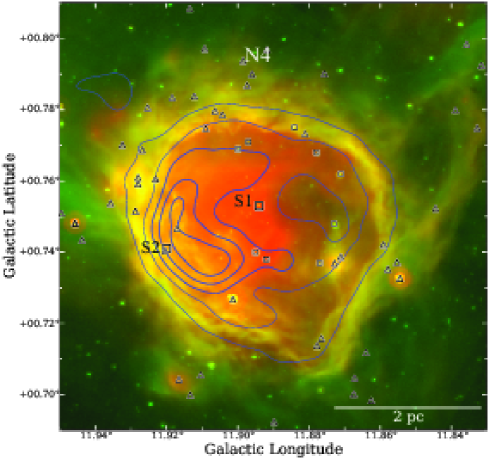
Figure 14: Closeup figure of Figure 1, but the blue contours show the intensity of 20-cm radio continuum taken from the Multi-Array Galactic Plane Imaging Survey (MAGPIS, Helfand et al. (2006)) archive ($b<0\fdg 8$), and are plotted by 0.75 ($\sim 5\sigma$), 1.95, 3.15, 4.35, and 5.55 mJy Beam^-1. Triangle symbols represent the YSOs identified by Liu et al. (2016).

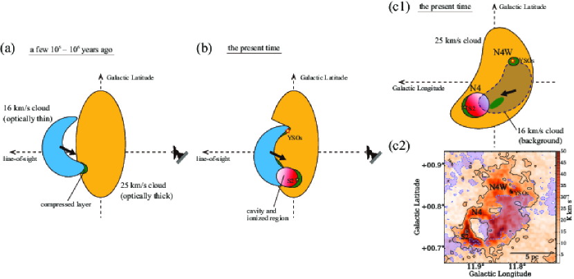
Figure 15: (a) Sketched diagrams of N4 and N4W as viewed from the Galactic east when the collision started. Blue and orange show the 16-km s^-1 cloud and the 25-km s^-1 cloud, respectively. Green region indicates the compressed layer between the two clouds, where star(s) form. (b) The sketched diagrams of N4 and N4W as viewed from the Galactic east at the present. Red indicates ionized region. (c1) The sketched diagrams of N4 and N4W on the sky view. (c2) Color scale shows the ¹³CO ($J$=1–0) integrated intensity of the 25-km s^-1 cloud (15 K km s^-1). Blue contours shows the ¹²CO ($J$=1–0) integrated intensity of the 16-km s^-1 cloud (12 K km s^-1).

4.5 Comparison of the molecular clouds and massive stars in N4 with those of the other massive-star forming regions

In Table 1, we compare the properties of the colliding molecular clouds in N4 with those of the other massive star-forming regions of RCW 120, RCW 38, and W51A that are also suggested to feature CCC. Spitzer bubble RCW 120 is comparable to N4 in terms of size and its ring appearance in near-IR. RCW 38 is known as a super star cluster. Fukui et al. (2016) suggested that the formation of multiple O-stars was triggered at the point of collision of two clouds. The spatial distributions of these two colliding clouds resemble those of the 16-km s^-1 cloud and the 25-km s^-1 cloud in N4. W51A is the one of the most active star-forming region in the Galaxy. Multiple previous studies (e.g., Carpenter & Sanders (1998); Okumura et al. (2001); Fujita et al. (2017)) suggested that a number of velocity components in W51A have been continuously colliding with each other, resulting in active massive star formation.

Fukui et al. (2018a) suggested that the molecular column density [$N({\rm H_{2}})$] of the colliding clouds can be an important parameter for determining the number of the end produce of O-stars. $N({\rm H_{2}})$ and the number of O-stars between N4 and RCW 120 were approximately the same, whereas the mass of the associated molecular clouds of RCW 120 were larger by a factor of $\sim$3. On the contrary, the number of O-stars in RCW 38 is much larger ($\sim$20), although the mass of the associated molecular clouds of RCW 38 is approximately same as that of N4. This could be attributed to the higher $N({\rm H_{2}})$ in RCW 38. In W51A, multiple collisions of clouds with high $N({\rm H_{2}})$ resulted in active massive star formation. The relationship between the $V_{\rm LSR}$ separations and the number of O-stars can not be discussed from these data. To establish a quantitative scenario for forming massive stars via a CCC, more observational studies and statistical studies are required.

Table 1: Properties of the colliding molecular clouds associated with N4, RCW120, RCW 38, and W51A

Name	Number of O-stars	Cloud Mass	Typical $N({\rm H_{2}})$	$V_{\rm LSR}$ Separation	Age of Hii region	References
		($10^{4}\ M_{\odot}$)	($10^{22}\ {\rm cm^{-2}}$)	(km s-1)	(Myr)
N4	$\sim$1 (O8.5–O9V†)	(1.7, 0.1)	(3–4, 0.3)	9	$\sim$0.4	This study
RCW 120	1 (O8–O9V)	(5.0, 0.4)	(3, 0.8)	20	$\sim$0.2	Torii et al. (2015)
RCW 38	$\sim$20 O-stars	(2.0, 0.3)	(10, 1)	12	$\sim$0.1	Fukui et al. (2016)
W51A	$\sim$30 O-stars	(11, 13, 19, 13)	$\sim$10 each	6–18	several 0.1	Fujita et al. (2017)

Note. — $\dagger$ Liu et al. (2016)

5 Summary

Using the FUGIN ¹²CO ($J$=1–0), ¹³CO ($J$=1–0), and the JCMT ¹²CO ($J$=3–2) datasets we studied the molecular gas distribution and velocity structure toward the Spitzer bubble N4 and N4W. The main results and conclusions are summarized below.

1. We observed three discrete velocity clouds: the 16-, 19-, and 25-km s^-1 clouds. Their molecular masses are $0.12\pm 0.02\times 10^{4}$ $M_{\odot}$, $0.43\pm 0.06\times 10^{4}$ $M_{\odot}$, and $3.8\pm 0.6\times 10^{4}$ $M_{\odot}$, respectively. The 16- and 19-km s^-1 clouds have not been recognized in previous observations of molecular lines. The distribution of the 25-km s^-1 cloud likely traces the ring-like structure observed in the mid-IR wavelength such as 8$\mu$m.

2. The 16- and 25-km s^-1 clouds are associated with the Hii region, whereas the 19-km s^-1 cloud is probably not interacting with N4 and N4W.

3. We investigated the velocity structure of the molecular clouds associated with the ring in N4, and could not find clear expanding motion.

4. We found two observational signatures of CCC (bridge features and complementary distributions) between the 16- and 25-km s^-1 clouds in N4. Therefore, we proposed a scenario in which a collision between the two clouds triggered the formation of the massive star candidates in N4 over a short timescale of only $\sim$0.3 Myr. This CCC scenario can explain the formation of both the molecular ring structure and massive star(s) inside the ring.

5. We also observed a bridge feature between the 16- and 25-km s^-1 clouds also in N4W. The CCC scenario in which massive- or intermediate-mass star formation was triggered by collision between the clouds is therefore also conceivable in N4W.

6. Both the massive star forming activity and the molecular column density in N4 were comparable to those of RCW120, whose molecular gas distribution also resembles that of N4. The number of O-stars formed via CCC may be related to their molecular column densities rather than to their molecular masses.

Appendix A Velocity channel maps of the ¹³CO ($J$=1–0) emissions

Figure 16 shows the large-scale velocity channel maps of the ¹³CO ($J$=1–0) emissions at a velocity step size of 2.6 km s^-1.

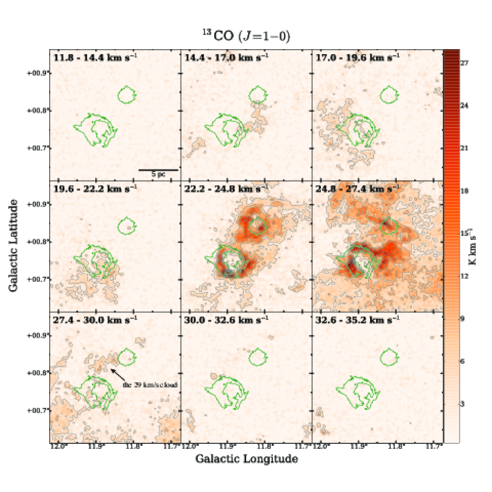
Figure 16: Same as Figure 3 but for the ¹³CO ($J$=1–0) emission. Black contours are plotted at every 4.0 K km s^-1 from 4.0 K km s^-1 ($\sim 5\sigma$).

References

- Anathpindika (2010) Anathpindika, S. V. 2010, MNRAS, 405, 1431
- Arce et al. (2011) Arce, H. G., Borkin, M. A., Goodman, A. A., Pineda, J. E., & Beaumont, C. N. 2011, ApJ, 742, 105
- Astropy Collaboration et al. (2013) Astropy Collaboration, Robitaille, T. P., Tollerud, E. J., et al. 2013, A&A, 558, A33
- Carpenter & Sanders (1998) Carpenter, J. M., & Sanders, D. B. 1998, AJ, 116, 1856
- Chen et al. (2016) Chen, Z., Zhang, S., Zhang, M., et al. 2016, ApJ, 822, 114
- Chen et al. (2017) Chen, Z., Jiang, Z., Tamura, M., Kwon, J., & Roman-Lopes, A. 2017, ApJ, 838, 80
- Churchwell et al. (2006) Churchwell, E., Povich, M. S., Allen, D., et al. 2006, ApJ, 649, 759
- Churchwell et al. (2007) Churchwell, E., Watson, D. F., Povich, M. S., et al. 2007, ApJ, 670, 428
- Colombo et al. (2015) Colombo, D., Rosolowsky, E., Ginsburg, A., Duarte-Cabral, A., & Hughes, A. 2015, MNRAS, 454, 2067
- Currie & Sicilia-Aguilar (2011) Currie, T., & Sicilia-Aguilar, A. 2011, ApJ, 732, 24
- Deharveng et al. (2009) Deharveng, L., Zavagno, A., Schuller, F., et al. 2009, A&A, 496, 177
- Deharveng et al. (2010) Deharveng, L., Schuller, F., Anderson, L. D., et al. 2010, A&A, 523, A6
- Elmegreen & Lada (1977) Elmegreen, B. G., & Lada, C. J. 1977, ApJ, 214, 725
- Enokiya et al. (2018) Enokiya, R., Sano, H., Hayashi, K., et al. 2018, PASJ, 70, S49
- Frerking et al. (1982) Frerking, M. A., Langer, W. D., & Wilson, R. W. 1982, ApJ, 262, 590
- Fujita et al. (2017) Fujita, S., Torii, K., Kuno, N., et al. 2017, arXiv:1711.01695
- Fukui et al. (2014) Fukui, Y., Ohama, A., Hanaoka, N., et al. 2014, ApJ, 780, 36
- Fukui et al. (2015) Fukui, Y., Harada, R., Tokuda, K., et al. 2015, ApJ, 807, L4
- Fukui et al. (2016) Fukui, Y., Torii, K., Ohama, A., et al. 2016, ApJ, 820, 26
- Fukui et al. (2018a) Fukui, Y., Torii, K., Hattori, Y., et al. 2018a, ApJ, 859, 166
- Fukui et al. (2018b) Fukui, Y., Kohno, M., Yokoyama, K., et al. 2018b, PASJ, 70, S60
- Fukui et al. (2018c) Fukui, Y., Ohama, A., Kohno, M., et al. 2018c, PASJ, 70, S46
- Furukawa et al. (2009) Furukawa, N., Dawson, J. R., Ohama, A., et al. 2009, ApJ, 696, L115
- Habe & Ohta (1992) Habe, A., & Ohta, K. 1992, PASJ, 44, 203
- Hayashi et al. (2018) Hayashi, K., Sano, H., Enokiya, R., et al. 2018, PASJ, 70, S48
- Haworth et al. (2015a) Haworth, T. J., Tasker, E. J., Fukui, Y., et al. 2015a, MNRAS, 450, 10
- Haworth et al. (2015b) Haworth, T. J., Shima, K., Tasker, E. J., et al. 2015b, MNRAS, 454, 1634
- Helfand et al. (2006) Helfand, D. J., Becker, R. H., White, R. L., Fallon, A., & Tuttle, S. 2006, AJ, 131, 2525
- Inoue & Fukui (2013) Inoue, T., & Fukui, Y. 2013, ApJ, 774, L31
- Inoue et al. (2018) Inoue, T., Hennebelle, P., Fukui, Y., et al. 2018, PASJ, 70, S53
- Kawada et al. (2007) Kawada, M., Baba, H., Barthel, P. D., et al. 2007, PASJ, 59, S389
- Kohno et al. (2018) Kohno, M., Torii, K., Tachihara, K., et al. 2018, PASJ, 70, S50
- Kuno et al. (2011) Kuno, N., et al. 2011, General Assembly and Scientific Symposium, XXXth URSI, JP2-19
- Leung et al. (1984) Leung, C. M., Herbst, E., & Huebner, W. F. 1984, ApJS, 56, 231
- Li et al. (2013) Li, J.-Y., Jiang, Z.-B., Liu, Y., & Wang, Y. 2013, Research in Astronomy and Astrophysics, 13, 921-934
- Liu et al. (2016) Liu, H.-L., Li, J.-Z., Wu, Y., et al. 2016, ApJ, 818, 95
- Martins et al. (2005) Martins, F., Schaerer, D., & Hillier, D. J. 2005, A&A, 436, 1049
- Minamidani et al. (2016) Minamidani, T., Nishimura, A., Miyamoto, Y., et al. 2016, Proc. SPIE, 9914, 99141Z s
- Nishimura et al. (2017) Nishimura, A., Costes, J., Inaba, T., et al. 2017b, arXiv:1706.06002
- Nishimura et al. (2018) Nishimura, A., Minamidani, T., Umemoto, T., et al. 2018, PASJ, 70, S42
- Ohama et al. (2010) Ohama, A., Dawson, J. R., Furukawa, N., et al. 2010, ApJ, 709, 975
- Ohama et al. (2018a) Ohama, A., Kohno, M., Hasegawa, K., et al. 2018a, PASJ, 70, S45
- Ohama et al. (2018b) Ohama, A., Kohno, M., Fujita, S., et al. 2018b, PASJ, 70, S47
- Okumura et al. (2001) Okumura, S.-I., Miyawaki, R., Sorai, K., Yamashita, T., & Hasegawa, T. 2001, PASJ, 53, 793
- Reid et al. (2016) Reid, M. J., Dame, T. M., Menten, K. M., & Brunthaler, A. 2016, ApJ, 823, 77
- Robitaille & Bressert (2012) Robitaille, T., & Bressert, E. 2012, Astrophysics Source Code Library, ascl:1208.017
- Rosolowsky et al. (2008) Rosolowsky, E. W., Pineda, J. E., Kauffmann, J., & Goodman, A. A. 2008, ApJ, 679, 1338
- Sano et al. (2017) Sano, H., Torii, K., Saeki, S., et al. 2017, arXiv:1708.08149
- Sano et al. (2018) Sano, H., Enokiya, R., Hayashi, K., et al. 2018, PASJ, 70, S43
- Shimoikura et al. (2013) Shimoikura, T., Dobashi, K., Saito, H., et al. 2013, ApJ, 768, 72
- Solarz et al. (2016) Solarz, A., Takeuchi, T. T., & Pollo, A. 2016, A&A, 592, A155
- Spitzer (1978) Spitzer, L. 1978, Physical processes in the interstellar medium, by Lyman Spitzer. New York Wiley-Interscience, 1978. 333 p.,
- Takahira et al. (2014) Takahira, K., Tasker, E. J., & Habe, A. 2014, ApJ, 792, 63
- Takahira et al. (2017) Takahira, K., Shima, K., Tasker, E. J., & Habe, A. 2017,
- Tan et al. (2014) Tan, J. C., Beltrán, M. T., Caselli, P., et al. 2014, Protostars and Planets VI, 149
- Torii et al. (2011) Torii, K., Enokiya, R., Sano, H., et al. 2011, ApJ, 738, 46
- Torii et al. (2015) Torii, K., Hasegawa, K., Hattori, Y., et al. 2015, ApJ, 806, 7
- Torii et al. (2017a) Torii, K., Hattori, Y., Hasegawa, K., et al. 2017a, ApJ, 835, 142
- Torii et al. (2017b) Torii, K., Hattori, Y., Matsuo, M., et al. 2017b, arXiv:1706.07164
- Torii et al. (2017c) Torii, K., Hattori, Y., Hasegawa, K., et al. 2017c, ApJ, 840, 111
- Torii et al. (2018) Torii, K., Fujita, S., Matsuo, M., et al. 2018, PASJ, 70, S51
- Tsuboi et al. (2015) Tsuboi, M., Miyazaki, A., & Uehara, K. 2015, PASJ, 67, 109
- Tsutsumi et al. (2017) Tsutsumi, D., Ohama, A., Okawa, K., et al. 2017, arXiv:1706.05664
- Umemoto et al. (2017) Umemoto, T., Minamidani, T., Kuno, N., et al. 2017, PASJ, 69, 78
- Watson et al. (2010) Watson, C., Hanspal, U., & Mengistu, A. 2010, ApJ, 716, 1478
- Wilson & Rood (1994) Wilson, T. L., & Rood, R. 1994, ARA&A, 32, 191
- Wu et al. (2004) Wu, Y., Wei, Y., Zhao, M., et al. 2004, A&A, 426, 503
- Zavagno et al. (2010) Zavagno, A., Russeil, D., Motte, F., et al. 2010, A&A, 518, L81
- Zinnecker & Yorke (2007) Zinnecker, H., & Yorke, H. W. 2007, ARA&A, 45, 481