Residual Memory Networks: Feed-forward approach to learn
long temporal dependencies

Abstract

Training deep recurrent neural network (RNN) architectures is complicated due to the increased network complexity. This disrupts the learning of higher order abstracts using deep RNN. In case of feed-forward networks training deep structures is simple and faster while learning long-term temporal information is not possible. In this paper we propose a residual memory neural network (RMN) architecture to model short-time dependencies using deep feed-forward layers having residual and time delayed connections. The residual connection paves way to construct deeper networks by enabling unhindered flow of gradients and the time delay units capture temporal information with shared weights. The number of layers in RMN signifies both the hierarchical processing depth and temporal depth. The computational complexity in training RMN is significantly less when compared to deep recurrent networks. RMN is further extended as bi-directional RMN (BRMN) to capture both past and future information. Experimental analysis is done on AMI corpus to substantiate the capability of RMN in learning long-term information and hierarchical information. Recognition performance of RMN trained with 300 hours of Switchboard corpus is compared with various state-of-the-art LVCSR systems. The results indicate that RMN and BRMN gains 6 % and 3.8 % relative improvement over LSTM and BLSTM networks.

Index Terms: Automatic speech recognition, LSTM, RNN, Residual memory networks.

1 Introduction

Automatic speech recognition (ASR) has largely improved using recurrent neural network (RNN) acoustic models due to the networks ability to learn long-term information. Unfortunately, RNNs becomes difficult to train when extended to deeper structure. This is because the deeper models is essential to learn more abstract information for improving the prediction of unseen data [1]. Several attempts have been made to train deep RNN such as using non-recurrent structures to increase the number of layers and model complexity [2], including transform gates for smoother gradient flow [3]. But training deep recurrent structures is complex as the gradient has to travel multiple hidden states and lack of better optimization algorithms [2]. Meanwhile, deep neural networks (DNN) can run much deeper, lead to better generalization to unseen data and are less prone to overfitting. Also, feed-forward training is relatively simple and faster when compared to recurrent structures. Besides these advantages, DNN fail to perform better for tasks which require long-term information. Thus to overcome this constraint, the authors in [4] represented the temporal context as a fixed size representation and train them jointly. In another work by [5, 6], the unweighted average of input context is used in modeling temporal information. The limitation with these approaches are that they fail to model the temporal order which is important for speech tasks as shown in [7]. Analogous to these networks is time delay neural network (TDNN), where each layer is fed with multi spliced input [8]. Even though TDNN has the ability to model long-term contexts, RNN still shows better performance over TDNN [8]. A possible reason for this is the fact that the performance gain of RNN is devoted to their stepwise learning of time frames and not by the size of context as found in [9].

A straight forward approach to allow DNN to learn a single time step at each layer is by denoting the time context length based on the number of layers. A practical challenge in this approach is that DNN having more than few layers starts to degrade due to gradient vanishing problem. Recent works by [10] showed that deeper convolutional networks can be trained in a much simpler way using residual connections. This approach showed significant gains in image recognition tasks. Additionally, [11] suggested to use shortcut connections and singular value decomposition for deeper fully connected networks and got better performance in ASR tasks. This paper makes an attempt to use residual structure with time delayed connections to harness the power of both temporal and hierarchical structures at each layer as explained in section 2. Figure 1, illustrates an basic form of residual network structure where the input $x$ is summed to next layers output using a shortcut connection with identity mapping $I$.

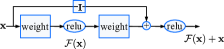
Figure 1: Structure of residual component

In this work, we propose Residual memory network (RMN), a variant of DNN where the number of layers denotes both the length of temporal information learnt and the structural depth. The key contributions of RMN are:

• The use of residual connections after every few layers to increase the network depth makes training faster with increase in performance. During backpropagation, the residual lines allows unimpeded flow of gradients.

• A memory component is present in each layer in a serial manner where the first layer sees $t-T$ time instant and the last layer sees $t-1$ frame. The component weights are shared across all layers to enable them to learn longer-context.

A combination of these two components allows RMN to learn long-term dependencies and higher level abstracts simultaneously in a much simpler and efficient way. Bi-directional RMN (BRMN) is also formulated in this work, which is a simple extension to RMN by adding an extra connection with shared weights for learning future information. Computational complexity is relatively less for BRMN over BLSTM or bi-directional RNNs which is detailed in section 2.1.

In section 3, we explain about AMI corpus and the baseline model configurations used in our experiments. A detailed explanation to build proposed RMN and BRMN model is in section 3.3 and 3.4. Empirical evaluation is conducted in section 4 to validate the structure of RMN for speech recognition tasks. Comparison of the RMN with the best LVCSR systems in literature in listed in section 4.4, which is followed by conclusion and future work.

2 Residual memory networks

RMN is composed of memory layers and residual connections as shown in figure 2. The residual connection connects the previous output to the current input by skipping few layers. Each memory layer contains two weight transforms: The first affine transform $W_{l}$ learns current time step and is different for each layer $l=1,2,..L$ as in standard DNNs. The second weight transform $W_{s}$ is shared across all layers and learns past information by varying delay in decreasing order. For example in figure 2, $W_{s}$ receives $t-T^{th}$ frame in first layer, second layer receives $t-(T-1)^{th}$ frame and the delay keep decreasing as we proceed to higher layers. In RMN $T$ is fixed based on the number of layers. For instance 18 layered network captures 18 time steps. In this network, relu activation is used after each memory layer as it is efficient for training deeper networks [11, 10]. Thus, RMN can be represented as a variant of deep feed-forward neural network which harnesses the important characteristics of unfolded-RNN and residual networks.

2.0.1 Forward propagation

Figure 2 shows the series of computations done in RMN architecture, where input $x(t),\,\{t=1,2,..T\}$ at time instant $t$ is processed using $W_{l}$ matrix in the layer $l$ to get $h_{l}(t)$. The shared weight $W_{s}$ receives $h_{l}(t-m)$ by delaying $h_{l}(t)$ by $m$ time steps. The feed-forward output after each memory layer is

$$y_{l}(t)=\phi\,(x(t)W_{l}+h_{l}(t-m)W_{s}),\,l=1,2,..L$$ (1)

where $h_{l}(t)=x(t)W_{l}$ and $\phi$ is the relu activation output.

2.0.2 Backward propagation

Backpropagation for computing the parameter $W_{l}$ is done in the same way as in standard DNNs. The shared parameter $W_{s}$ is computed by taking into account error gradients from all $T$ time instants which is exactly equal to $L$ memory layers. The error derivative w.r.t to $W_{s}$ is

$$\frac{\partial E(t)}{\partial W_{s}}=\sideset{}{{}_{k=1}^{T}}{\sum}\left[\frac{\partial E(t)}{\partial\hat{z}(t)}\frac{\partial\hat{z}(t)}{\partial h_{l}(t)}\right]\frac{\partial h_{l}(t)}{\partial h_{k}(k)}\frac{\partial h_{k}(k)}{\partial W_{s}}$$ (2)

where $\hat{z}(t)$ is the softmax output,$z(t)$ is target label and $E_{t}(.)$ denotes cross-entropy loss function.

2.1 Bi-directional residual memory network

In this section, the structure of bi-directional RMN (BRMN) is discussed. The BRMN is an extension of RMN with one additional shared weight transform which receives future frames as input. The forward propagation output is given as

$$y_{l}(t)=\phi\,(x(t).W_{l}+h_{l}(t-m).W_{s}+h_{l}(t+m).W_{b})$$ (3)

where $t-m$ is the time instant delayed by m steps and $W_{b}$ is the shared weight across layers. Unlike bi-directional RNN described in [12], BRMN does not require two separate recurrent units for training future and past frames. The past and future frames are not treated as independent entities and merged after each layer. A possible explanation for bi-directional RNN to have two separate layers is because RNN is tend to look over all frames during prediction which leads to performance drop[12]. In case of BRMN the network is constrained to pre-defined context size based on the the number of memory layers and thus connecting the forward states and backward states after each memory layer shows improvement in performance. Also, BRMN requires only one extra weight transform over RMN and hence the number of parameters is significantly less when compared to bi-directional RNN and BLSTM [13, 12].

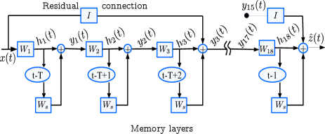
Figure 2: Architecture of residual memory network (RMN) with number of memory layers $L=18.$ The memory layers can model temporal context size of 18.

3 Experimental setup

The experiments were conducted on the AMI meeting conversation corpus , using the independent headset microphone (IHM) recordings. The database is composed of 77 hours - train data and 9 hours of each dev and eval data. 16KHz sampled waveform was used to extract 13-dimensional MFCC features. These features were mean normalized, spliced over 7 frames and projected down to 40 dimensions using linear discriminant analysis (LDA) obtained from LDA+MLLT model. The LDA features were fed to speaker adaptive training (SAT) using speaker based feature-space maximum likelihood linear regression (fMLLR) transforms to obtain fMLLR features. 80 dimensional log Mel-filterbank (fbank) features were also used for comparison. The standard GMM-HMM and DNN is trained by following the Kaldi toolkit [14]. The LSTM and RMN is trained using the CNTK toolkit [15]. SAT alignments using 4006 tied-states were used as targets for neural network training. Testing was done using eval set with trigram language model.

3.1 Baseline DNN and LSTM models

The DNN configuration includes 440 (40 x 11 splice) dimensional fMLLR features at input and 4006 senones at softmax output. DNN containing 6 hidden layers, 2048 neurons were initialized using RBM pretraining and fine-tuned with minibatch SGD frame-classification training. The LSTM training is performed by following the CNTK recipe [16]. The LSTM is composed of 3 projected LSTM layers, each having 1024 memory cells and 512 projection units. The LSTM is trained using truncated backpropagation through time (BPTT) with a minibatch size of 20. Forward propagation is done with 40 parallel utterances for faster training and better generalization [15]. Highway LSTM is also built by following the procedure in [3] to analyze the effect of increase in LSTM depth. 3 layered Highway LSTM works better as increasing it to 8 degrades the performance as in table 3. Further experiments in this paper is done with 3 layered Highway LSTM and will be denoted as LSTM for simplicity. The BLSTM architecture is also used which include 3 bi-directional layers each with 512 memory cells and 300 projection units. BLSTM is trained using latency control technique with 22 past frames and 21 future frames as mentioned in [3]. The LSTM based models receives 40 dimensional fMLLR directly as splicing does not help for training LSTMs [17]. The speech recognition results of all these models are stated in table 3.

3.2 Ivector extractor

BUT standardization initiative tool is used an ivector extractor. This extractor is trained on 9000 hours of Fisher English (part 1 and 2), NIST SRE 2004-2008, Switchboard (phase 2, phase 3, cellular part 1, and cellular part 2). An 100 dimensional mean- and length-normalized ivector is extracted for each speaker, after applying multi-lingual neural network based VAD tuned to detect confident speech. Ivectors are appended to input features for training LSTM based systems as suggested in [16].

3.3 RMN configuration and training

The memory layers in the RMN architecture contains 512 hidden units followed by the relu activation function. The memory layer is preceded and followed by a higher dimensional layer of 1024 units as it was found to be crucial for better learning. Thus the network configuration is represented as 440-1024- [512 x N layers]-1024-4006. The separate weights of RMN $W_{l}$ as mentioned in section 2 are Gaussian initialized with mean $0$ and standard deviation of $0.2/\sqrt{layer\,dim}$. The shared weight matrix $W_{s}$ is initialized as $0$ to ensure the model learns feature representation during the first epoch followed by learning of temporal information. This is done to disable the transfer of delayed inputs at the beginning of training. Also, empirically we found that we can restrict the matrix $W_{s}$ to be diagonal without loss in performance and it was used throughout this work. In RMN, the residual connection shown is created after every 3 layers as we found it to be optimum as in table 3. Thus RMN requires smaller number of parameters compared to standard DNN and LSTM as mentioned in table 4. The RMN is trained using truncated BPTT with a minibatch size of 256 as suggested in [18] and a maximum of 10 utterances in each minibatch. The initial learning rate is set to 0.2 and increased to 1 in the next 4 epochs. Further training is done by automatically reducing the learning rate for the next epoch by a factor of 0.5 if cross-entropy loss degrades. L2 regularization weight is fixed to 0.00001 and momentum is set to 0.9. The scripts for running the RMN and BRMN experiments are available in github repository

3.4 BRMN configuration and training

The bi-directional RMN (BRMN) is trained by following the same procedure as RMN with the following modifications: First, the initial learning rate is fixed as 0.000095 and then allowed to auto adjust [15] based on validation loss as in RMN. Second, latency control technique is used to capture 21 future frames. Empirically, we found that BRMN works better for non-spliced input i.e., 40 dimensional fMLLR features were directly sent to input of BRMN. Table 3 shows the performance BRMN with and without splicing. Thus the network configuration of BRMN is 40-1024-[512 x 18 layers]-1024-4006.

Table 1: Baseline recognition performance (% WER) of DNN, DNN+residual, LSTM, highway LSTM and BLSTM for eval set of AMI corpus using fMLLR features

DNN	DNN+	LSTM [16]	Highway LSTM		BLSTM
	residual	3 layers	3 layers	8 layers	3 layers
27.1	26.7	26.0	25.8	26.0	24.9

Table 2: % WER of RMN model with number of layers skipped by the residual connection. This experiment is done by with 15 memory layers of RMN

# layers skipped by residue
1	2	3	4
26.6	26.0	25.9	25.9

Table 3: % WER of RMN and BRMN for spliced and non-spliced input with different width using eval set of AMI corpus

% WER	Splice width
Model	1 (no splice)	15 (+/-7)	21 (+/-10)
RMN	26.6	25.6	25.6
BRMN	24.3	24.8	25.4

4 Validation experiments

This section provides a detailed analysis to understand the behavior of RMN.

4.1 Effect on layer size and feature type

Initial experiment is done to find the optimum number of layers for RMN using 40 dimensional fMLLR features. Figure 3 compares the performance of DNN + residual networks with and without delay connections. The baseline performance of DNN+residual without delay is shown in table 3 Two notable observations can be made from this figure. 1) The importance of delay connections is clearly visible from this figure as it shows more than 1% absolute gain over DNN+residual models. 2) The increase in number of layers has positive influence over both DNN+residual and RMN systems. The performance of both systems reaches threshold after 18 layers. Based on these observations, the number of optimum RMN layers is chosen to 18.

Table 4 shows the effect of fMLLR features and fbank features using RMN. This table shows that RMN shows comparable performance to LSTM using fbank features. The performance of RMN is clearly better for fMLLR features when compared to fbank features. The LSTM models seems to perform slightly better over RMN systems for fbank features. It is also visible that both RMN and LSTM suffers with fbank due to the existence of strong correlations in time and frequency. Thus, further experiments in this paper will be conducted based on fMLLR features.

4.2 Effect of bi-directional RMN and parameters

Table 4 shows that the BRMN model gains absolute 1.3 % improvement over RMN. Next, it is observed that RMN shows slight improvement over LSTM and a similar pattern is noted in bi-directional models. A striking difference between RMN and LSTM models is the number of computational parameters. Even though the RMN has deeper structure the number of parameters is greatly reduced. From table, it is visible that RMN requires 28.9 % lesser parameters than LSTM while BRMN needs 38.5 % lesser parameters than BLSTM. The reason behind this parameter difference in BRMN is due to its simple addition of one extra weight transform for future frames over RMN model, while BLSTM requires two separate LSTM layers for both directions.

Figure 3: Performance comparison between RMN and (DNN+residual) networks for different layer sizes

To verify the importance of deeper architecture in reducing data mismatch, the training and validation error is plotted in figure 4. Convergence of RMN model indicates that RMN is learning in a similar fashion as LSTM. The training loss of RMN models is more than when compared to LSTM models, substantiating that RMN is less prone to overfitting. In case of validation loss, RMN models shows less error over LSTM based systems.

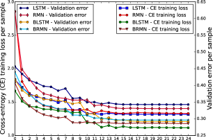
Figure 4: Training and validation err on RMN, BRMN, LSTM and BLSTM using AMI corpus

4.3 Speaker adaptation using ivectors

The RMN is fed with ivectors by augmenting it with input features. The experiments in table 4 shows that RMN with fMLLR+ivector features gives 6.25 % relative improvement over RMN with fMLLR. A relative improvement of 7.4 % is obtained by BRMN model using fMLLR+ivector over fMLLR features. A minimal improvement of absolute 0.3 % is obtained for RMN over LSTM network. The BRMN system with ivectors provides 1.75 % relative improvement over BLSTM with ivectors. Augmenting ivectors in BLSTM increases the parameters by 2 million whereas BRMN parameters are increased by 0.1 million. This signifies that BRMN shows significant gains over BLSTM without increasing the parameters drastically.

Table 4: Comparison of LSTM and RMN with uni- and bi-directional layers and different types of features. Performance of speaker adaptation using ivectors is noted here. The number of parameters (# params) computed is also listed.

Input	Model	Uni-directional		Bi-directional
		% WER	# params	% WER	# params
Fbank	LSTM	27.8	14.5 M	26.3	17.1 M
	RMN	28.1	10.7 M	26.4	9.9 M
fMLLR	LSTM	25.8	14.5 M	24.5	16.1 M
	RMN	25.6	10.3 M	24.3	9.9 M
fMLLR+	LSTM	24.3	16.5 M	22.9	18.1 M
ivec	RMN	24.0	10.4 M	22.5	10.0 M

Table 5: Comparison of RMN with existing methods in literature trained using 300 hours of Switchboard corpus and tested with Hub5-00 eval set. In this table 3g is trigram, 4g is meant as 4-gram, bn-fMLLR is bottleneck features with fMLLR and ivec represents 100 dimensional ivectors built using section 3.2.

% WER	Model Type	SWB (% CE WER)
		3g	4g	4g+ivec
Proposed	RMN	13.0	12.0	10.9
Models	BRMN	11.8	10.8	9.9
State-of-the-art	TDNN [19]			12.5
results	Unfolded RNN + fMLLR [18]			12.7
in	LSTM + bn-fMLLR [20]			10.8
literature	LSTM [19]			11.6
	BLSTM [19]			10.3

4.4 Results of various LVCSR systems

This section brings the state-of-the-results of LSTM, BLSTM, unfolded RNN and TDNN models using 300 hours of switchboard data tested with hub5-2000 evaluation set. These results are obtained by using ivectors and 4-gram language model. To present a fair comparison, RMN model is also trained with 300 hours data followed by testing with a trigram language model built with Fisher and switchboard corpus, and later rescored with 4-gram language model. The RMN and BRMN is trained in a similar configuration as mentioned in section 3.3 and 3.4. The table 5 shows the % WER of switchboard (SWB) subset obtained after cross-entropy (CE) training. The effectiveness of RMN in modeling long-term dependencies for large vocabulary data is clearly visible in table 5.

5 Conclusion

In this paper we proposed residual memory network (RMN) structure, a variant of feed-forward network to capture temporal context. We have also introduced a bi-directional RMN which capture forward and backward states with less computational complexity. The reasonable effectiveness of RMN in capturing both temporal and higher-order information was shown in AMI and switchboard tasks. BRMN showed 3.8 % relative improvement over BLSTM and RMN gained 6 % relative improvement over LSTM. In the future, we will develop a way to further increase the depth of RMN for capturing longer context. A interesting direction is to validate the ability of RMN in language modeling tasks. To increase the efficiency of RMN with fbank features, we would like to use convolutional layers before RMN to learn spatial representations.

References

- [1] Hasim Sak, Andrew W Senior, and Françoise Beaufays, “Long short-term memory recurrent neural network architectures for large scale acoustic modeling.,” in INTERSPEECH, 2014, pp. 338–342.
- [2] Razvan Pascanu, Caglar Gulcehre, Kyunghyun Cho, and Yoshua Bengio, “How to construct deep recurrent neural networks,” arXiv preprint arXiv:1312.6026, 2013.
- [3] Yu Zhang, Guoguo Chen, Dong Yu, Kaisheng Yaco, Sanjeev Khudanpur, and James Glass, “Highway long short-term memory rnns for distant speech recognition,” in International Conference on Acoustics, Speech and Signal Processing (ICASSP), 2016, Shanghai, China. IEEE, 2016, pp. 5755–5759.
- [4] Shiliang Zhang, Cong Liu, Hui Jiang, Si Wei, Lirong Dai, and Yu Hu, “Feedforward sequential memory networks: A new structure to learn long-term dependency,” arXiv preprint arXiv:1512.08301, 2015.
- [5] Colin Raffel and Daniel PW Ellis, “Feed-forward networks with attention can solve some long-term memory problems,” arXiv preprint arXiv:1512.08756, 2015.
- [6] Karel Vesel, Shinji Watanabe, Martin Karafi, Jan Honza, et al., “Sequence summarizing neural network for speaker adaptation,” in International Conference on Acoustics, Speech, and Signal Processing (ICASSP), 2016, Shanghai, China. IEEE, 2016, pp. 5315–5319.
- [7] Sepp Hochreiter and Jürgen Schmidhuber, “Long short-term memory,” Neural computation, vol. 9, no. 8, pp. 1735–1780, 1997.
- [8] Vijayaditya Peddinti, Daniel Povey, and Sanjeev Khudanpur, “A time delay neural network architecture for efficient modeling of long temporal contexts,” in INTERSPEECH. ISCA, 2015, pp. 2440–2444.
- [9] Abdel-rahman Mohamed, Frank Seide, Dong Yu, Jasha Droppo, Andreas Stoicke, Geoffrey Zweig, and Gerald Penn, “Deep bi-directional recurrent networks over spectral windows,” in Automatic Speech Recognition and Understanding (ASRU). IEEE, 2015, pp. 78–83.
- [10] Kaiming He, Xiangyu Zhang, Shaoqing Ren, and Jian Sun, “Deep residual learning for image recognition,” arXiv preprint arXiv:1512.03385, 2015.
- [11] Pegah Ghahremani, Jasha Droppo, and Michael L Seltzer, “Linearly augmented deep neural network,” in International Conference on Acoustics, Speech, and Signal Processing (ICASSP), 2016, Shanghai, China. IEEE, 2016, pp. 5085–5089.
- [12] Mike Schuster and Kuldip K Paliwal, “Bidirectional recurrent neural networks,” IEEE Transactions on Signal Processing, vol. 45, no. 11, pp. 2673–2681, 1997.
- [13] Alex Graves and Navdeep Jaitly, “Towards end-to-end speech recognition with recurrent neural networks.,” in ICML, 2014, vol. 14, pp. 1764–1772.
- [14] Daniel Povey, Arnab Ghoshal, Gilles Boulianne, Lukas Burget, Ondrej Glembek, Nagendra Goel, Mirko Hannemann, Petr Motlicek, Yanmin Qian, Petr Schwarz, et al., “The kaldi speech recognition toolkit,” in Automatic Speech Recognition and Understanding, 2011 IEEE Workshop on. IEEE, 2011, pp. 1–4.
- [15] Dong Yu, Adam Eversole, Mike Seltzer, Kaisheng Yao, Zhiheng Huang, Brian Guenter, Oleksii Kuchaiev, Yu Zhang, Frank Seide, Huaming Wang, et al., “An introduction to computational networks and the computational network toolkit,” Tech. Rep., Technical report, Tech. Rep. MSR, Microsoft Research, 2014, 2014. research. microsoft. com/apps/pubs, 2014.
- [16] Tian Tan, Yanmin Qian, Dong Yu, Souvik Kundu, Liang Lu, Khe Chai Sim, Xiong Xiao, and Yu Zhang, “Speaker-aware training of lstm-rnns for acoustic modelling,” in International Conference on Acoustics, Speech and Signal Processing (ICASSP) 2016, Shanghai, China. IEEE, 2016, pp. 5280–5284.
- [17] Yajie Miao and Florian Metze, “On speaker adaptation of long short-term memory recurrent neural networks,” in INTERSPEECH, 2015.
- [18] George Saon, Hagen Soltau, Ahmad Emami, and Michael Picheny, “Unfolded recurrent neural networks for speech recognition.,” in INTERSPEECH, 2014, pp. 343–347.
- [19] Daniel Povey, Vijayaditya Peddinti, Daniel Galvez, Pegah Ghahrmani, Vimal Manohar, Xingyu Na, Yiming Wang, and Sanjeev Khudanpur, “Purely sequence-trained neural networks for asr based on lattice-free mmi,” INTERSPEECH, 2016.
- [20] George Saon, Tom Sercu, Steven J. Rennie, and Hong-Kwang Jeff Kuo, “The IBM 2016 english conversational telephone speech recognition system,” CoRR, vol. abs/1604.08242, 2016.