OptStream: Releasing Time Series Privately

Abstract

Many applications of machine learning and optimization operate on data streams. While these datasets are fundamental to fuel decision-making algorithms, often they contain sensitive information about individuals, and their usage poses significant privacy risks. Motivated by an application in energy systems, this paper presents OptStream, a novel algorithm for releasing differentially private data streams under the w-event model of privacy. OptStream is a 4-step procedure consisting of sampling, perturbation, reconstruction, and post-processing modules. First, the sampling module selects a small set of points to access in each period of interest. Then, the perturbation module adds noise to the sampled data points to guarantee privacy. Next, the reconstruction module re-assembles non-sampled data points from the perturbed sample points. Finally, the post-processing module uses convex optimization over the private output of the previous modules, as well as the private answers of additional queries on the data stream, to improve accuracy by redistributing the added noise. OptStream is evaluated on a test case involving the release of a real data stream from the largest European transmission operator. Experimental results show that OptStream may not only improve the accuracy of state-of-the-art methods by at least one order of magnitude but also supports accurate load forecasting on the private data.

1 Introduction

Differential privacy (?) has emerged as a robust framework to release datasets while limiting the disclosure of participating individuals. Informally, it ensures that what can be learned about an individual in a differential private dataset is, with high probability, limited to what could have been learned about the individual in the same dataset but without her data.

Many applications of machine learning and optimization, in areas such as healthcare, traffic management, and social networks, operate over streams of data. The use of differential privacy for the private release of time series has attracted increased attention in recent years (e.g., (?, ?, ?, ?, ?)) where aggregated statistics are continuously reported. Two common approaches for time series data release are the event-level and user-level privacy models (?). The former focuses on protecting a single event, while the latter aims at protecting all the events associated with a single user, i.e., it focuses on protecting the presence of an individual in the dataset. Additionally, ? (?) proposed the notion of $w$-event privacy to achieve a balance between event-level and user-level privacy, trading off utility and privacy to protect event sequences within a time window of $w$ time steps.

This paper was motivated by a desire to release private streams of energy demands, also called loads, in transmission systems. The goal is that of protecting changes in consumer loads up to some desired amount within critical time intervals. Although customer identities are typically considered public information (e.g., each facility is served by some energy provider), their loads can be highly sensitive as they may reveal the economic activities of grid customers. For example, changes in load consumption may indirectly reveal production levels and strategic investments and other similar information. Moreover, these time series are often input to complex analytic tasks, e.g., demand forecasting algorithms (?) and optimal power flows (?). As a result, the accuracy of the private datasets is critical and, as shown later in the paper, existing algorithms for time series fall short in this respect for this application.

The main contribution of this paper is a new privacy mechanism that remedies these limitations and is sufficiently precise for use in forecasting and optimization applications. The new algorithm, called OptStream, is presented under the framework of $w$-event privacy and is a 4-step procedure consisting of sampling, perturbation, reconstruction, and post-processing modules. The sampling module selects a small set of points for private measurement in each period of interest, the perturbation module introduces noise to the sampled data points to guarantee privacy, the reconstruction module reconstructs the non-sampled data points from the perturbed sampled points, and the post-processing module uses convex optimization over the private output of the previous modules, as well as the private answers of additional queries on the data stream, to redistribute the noise to ensure consistency of salient features of the data. OptStream is also generalized to answer queries over hierarchical streams, allowing data curators to monitor simultaneously streams produced by energy profile data at different levels of aggregation. It is important to emphasize that, although OptStream was motivated by an energy application, it is potentially useful for many other domains, since its design is independent of the underlying problem.

OptStream is evaluated on real datasets from Réseau de Transport d’Électricité, the French transmission operator and the largest in Europe. The dataset contains the energy consumption for one year at a granularity of 30 minutes. OptStream is also compared with state-of-the-art algorithms adapted to $w$-event privacy. Experimental results show that OptStream improves the accuracy of state-of-the-art algorithms by at least one order of magnitude for this application domain. The effectiveness of the proposed algorithm is measured, not only in terms of the error between the reported private streams and the original stream but also in the accuracy of a load forecasting algorithm based on the private data. Finally, the paper shows that the sampling and optimization-based post-processing steps are critical in achieving the desired performance and that the improvements are also observed when releasing hierarchical streams of data.

The rest of this paper is organized as follows. Section 2 discusses the stream model, summarizes the privacy goals of this work, and reviews the notion of differential privacy over streams. Section 3 describes OptStream and the design choices of its components. Section 4 analyzes the accuracy of the proposed framework and shows how it reduces the error introduced to preserve privacy when compared to a standard solution. Section 5 extends OptStream to the $\alpha$-indistinguishability privacy model, allowing privacy protection of arbitrary quantities and which is critical for the motivating application. Additionally, OptStream is extended to handle hierarchical stream data. Section 6 performs a comprehensive experimental analysis of real data streams from energy load profiles. Section 7 discusses key aspects of the privacy model adopted to privately releasing streams of data, as well as differences with the event-based model for data streams. Section 8 discusses the related work and, finally, Section 9 concludes the work.

2 Preliminaries

This section first reviews basic concepts in differential privacy. It then presents the $w$-event privacy model used to protect privacy in data streams and its definition of differential privacy.

2.1 Differential Privacy

This section reviews the standard definition of differential privacy (?). Differential privacy focuses on protecting the privacy of an individual user participating to a dataset. Such notion relies on the definition of a adjacency relation $\sim$ between datasets. Two datasets $X,X^{\prime}$ are called $neighbors$ if their content differs in at most one tuple: $X\sim X^{\prime}\;\Leftrightarrow\;\|X-X^{\prime}\|\leq 1$.

Definition​ 1 (Differential Privacy)

Let $\mathcal{A}$ be a randomized algorithm that takes as input a dataset and outputs an element from a set of possible responses. $\mathcal{A}$ achieves $\epsilon$-differential privacy if, for all sets $O\subseteq{\mathcal{O}}$ and all neighboring datasets $X,X^{\prime}\in\mathcal{D}$:

$$\frac{Pr[\mathcal{A}(X)\in O]}{Pr[\mathcal{A}(X^{\prime})\in O]}\leq\exp(\epsilon).$$ (1)

The level of privacy is controlled by the parameter $\epsilon\geq 0$, called the privacy budget, with values close to $0$ denoting strong privacy. The adjacency relation $\sim$ captures the participation of an individual into the dataset. While differential privacy algorithms commonly adopts the $1$-Hamming distance as adjacency relation between datasets, the latter can be generalized to be any symmetric binary relation $\sim\in\mathcal{D}^{2}$. In particular, the relation $\sim$ captures the aspects of the private data $D$ that are considered sensitive and has been generalized to protect locations of individuals (?) and quantities in general (?). When a single entry is associated with a user in the database, an algorithm satisfying Equation (1) prevents an attacker with access to the algorithm’s output from learning anything substantial about any individual.

2.1.1 Properties of Differential Privacy

Differential privacy enjoys several important properties, including composability and immunity to post-processing.

Composability

Composability ensures that a combination of differentially private algorithms preserve differential privacy (?).

Theorem​ 1 (Sequential Composition)

The composition $\mathcal{A}(D)=(\mathcal{A}_{1}(D),\ldots,\mathcal{A}_{k}(D))$ of a collection $\{\mathcal{A}_{i}\}_{i=1}^{k}$ of $\epsilon_{i}$-differentially private algorithms satisfies $(\sum_{i=1}^{k}\epsilon_{i})$-differentially privacy.

Theorem​ 2 (Parallel Composition)

Let $D_{1}$ and $D_{2}$ be disjoint subsets of $D$ and $\mathcal{A}$ be an $\epsilon$-differentially private algorithm. Then computing $\mathcal{A}(D\cap D_{1})$ and $\mathcal{A}(D\cap D_{2})$ satisfies $\epsilon$-differential privacy.

Post-processing Immunity

Post-processing immunity ensures that privacy guarantees are preserved by arbitrary post-processing steps (?).

Theorem​ 3 (Post-Processing Immunity)

Let $\mathcal{A}$ be an $\epsilon$-differentially private algorithm and $g$ be an arbitrary mapping from the set of possible output sequences ${\mathcal{O}}$ to an arbitrary set. Then, $g\circ\mathcal{A}$ is $\epsilon$-differentially private.

We now introduce two useful differentially private algorithms.

2.1.2 The Laplace Mechanism

A numeric query $Q$, mapping a dataset to $\mathbb{R}^{d}$, can be made differentially private by injecting random noise to its output. The amount of noise to inject depends on the sensitivity of the query, denoted by $\Delta_{Q}$ and defined as,

$$\Delta_{Q}=\max_{D\sim D^{\prime}}\left\|Q(D)-Q(D^{\prime})\right\|_{1}.$$

In other words, the sensitivity of a query is the maximum $L_{1}$-distance between the query outputs from any two neighboring dataset $D$ and $D^{\prime}$. For instance, $\Delta_{Q}=1$ for a query $Q$ that counts the number of users in a dataset.

The Laplace distribution with 0 mean and scale $b$, denoted by ${\text{Lap}}(b)$, has a probability density function ${\text{Lap}}(x|b)=\frac{1}{2b}e^{-\frac{|x|}{b}}$. It can be used to obtain an $\epsilon$-differentially private algorithm to answer numeric queries (?). In the following, we use ${\text{Lap}}(\lambda)^{d}$ to denote the i.i.d. Laplace distribution over $d$ dimensions with parameter $\lambda$.

Theorem​ 4 (Laplace Mechanism $\mathcal{M}_{\mathrm{Lap}}$)

Let $Q$ be a numeric query that maps datasets to $\mathbb{R}^{d}$. The Laplace mechanism that outputs $Q(D)+z$, where $z\in\mathbb{R}$ is drawn from the Laplace distribution $\textrm{{\text{Lap}}}\left(\frac{\Delta_{Q}}{\epsilon}\right)^{d}$, achieves $\epsilon$-differential privacy.

2.1.3 Sparse Vector Technique

The Sparse Vector Technique (SVT) is an important tool of differential privacy (?, ?) that allows to answer a sequence of queries without incurring a high privacy cost. The SVT mechanism is given a sequence of queries $Q=q_{1},q_{2},\ldots$ and a sequence of real valued thresholds $\Theta=\theta_{1},\theta_{2},\ldots$ and outputs a vector indicating whether each query answer $q_{i}$ is above or below the corresponding threshold $\theta_{i}$. In other words, the output is a vector $\{\top,\bot\}^{\ell}$ where $\ell$ is the number of queries answered and $\top$ (resp. $\bot$) indicates that the answer to a noisy query is (resp. is not) above a noisy threshold.

The SVT mechanism is summarized in Algorithm 1. It takes as input a dataset $D$, a sequence of queries $Q=q_{1},q_{2},\ldots$, each with sensitivity no more than $\Delta_{Q}$, a sequence of thresholds $\Theta=\theta_{1},\theta_{2},\ldots$, and a constant $k$, denoting the maximum number of queries to be answered with value $\top$. Its output consists of a sequence of answers $a_{1},a_{2},\ldots$ with each $a_{i}\in\{\top,\bot\}$. For each query, SVT perturbs the corresponding threshold and checks if the perturbed individual query answer is above the noisy threshold.

Theorem​ 5 (SVT)

The SVT mechanism achieves $\epsilon$-differential privacy (?).

The SVT mechanism is useful especially in situations when one expects that most answers fall below the threshold, since the noise depends on $k$. The SVT mechanism will be used in this paper to find good sampled points in a stream.

input : $D$: the dataset

$Q=q_{1},q_{2},\ldots$: a sequence of queries

$\Theta=\theta_{1},\theta_{2},\ldots$: a sequence of thresholds

$k$: the maximum number of queries to be answered positively

$\epsilon$: the privacy budget

1

2$\rho=Lap(2\Delta_{Q}/\epsilon)$;

3 count = 0;

4 foreach query $q_{i}\in Q$ do

5       $\nu_{i}=Lap(4k\Delta_{Q}/\epsilon)$;

6       if  $q_{i}(D)+\nu_{i}\geq\theta_{i}+\rho$ then

7             output $a_{i}=\top$;

8             count = count + 1;

9             Break if count $\geq k$;

10            

11      else

12             output $a_{i}=\bot$;

13            

14      

Algorithm 1 SVT - Sparse Vector Technique

2.2 The $w$-Event Privacy Model for Data Streams

This section presents the privacy model for streams adopted in this paper. A data stream $D$ is an infinite sequence of elements in the data universe ${\mathscr{U}}=\mathcal{I}\times\mathcal{T}$, where $\mathcal{I}$ denotes the set of user identifiers and $\mathcal{T}$ is a possibly unbounded set of time steps. In other words, each tuple $(i,t)$ describes an event reported by user $i$ that occurred at time $t$. Time is represented through discrete steps $\mathcal{T}=\{1,2,\ldots\}$ and user events are recorded periodically (e.g., every 30 minutes). In a data stream $D$, tuples are ordered by arrival time. If tuple $(i,t)$ arrives after tuple $(i^{\prime},t^{\prime})$, then $t\geq t^{\prime}$. Additionally, In the following, $D[t]$ denotes a stream prefix, i.e., the sequence $D_{1},\ldots,D_{t}$ of all tuples observed on or before time $t$. Additionally, $\mathcal{D}$ denotes the set of all datasets describing collections of tuples in ${\mathscr{U}}$.

Example​ 1

Consider a data stream system that collects location data from WiFi access points (APs) in a collection of buildings. Users correspond to MAC addresses of individual devices that connect to an AP. An item $(i,t)$ in the data stream represents that the fact that user $i$ has made at least one connection to an access point at time step $t$. In the following table, user 02:18:98:09:1a:a4 reports a connection at times $t=1$ and $t=2$. The example represents a data stream prefix $D[3]$.

$D_{1}$	$D_{2}$	$D_{3}$	…
02:18:98:09:1a:a4	02:18:98:09:1a:a4	05:12:11:0a:30:03
05:12:11:0a:30:03	05:12:11:0a:30:03	11:28:18:a9:1b:a3
11:28:18:a9:1b:a3	11:28:18:a9:1b:a3	07:22:1a:12:31:33
	07:22:1a:12:31:33	01:11:e2:14:43:b2
	01:11:e2:14:43:b2

The data curator receives information from an unbounded data stream $D$ in discrete time steps. At time $t$, the curator collects a dataset $D_{t}$ of tuples $(i,t)$ where every row corresponds to a unique user. The curator reports the result of a count query $Q:\mathcal{D}\to\mathbb{R}$ that reports how many users are in the dataset at time $t$, i.e., $Q(D_{t})=|\{i:(i,t)\in D_{t}\}|$.

Example​ 2

Consider the data stream prefix of Example 1. The associated result of the count queries executed onto each dataset of the data stream is given in the following table.

$Q(D_{1})$	$Q(D_{2})$	$Q(D_{3})$	…
3	5	4

In our target application, the data curator is interested in publishing every element $Q(D_{t})$ for a recurring period of $w$ time steps. A $w$-period is a set of $w$ contiguous time steps $t\!-\!w\!+\!1,\!\ldots,\!t$ ($w\!\geq\!1$). Thus, the answers to each query $Q(D_{t})$ are generated in real time for windows of $w$ time steps. As a result, this paper adopts the $w$-event privacy framework by ? (?).

2.3 Differential Privacy on Streams

The $w$-event privacy framework (?) extends the definition of differential privacy to protect data streams and has become a standard privacy notion for data streams (see, for instance, (?, ?, ?, ?, ?)). The framework operates on stream prefixes and two data streams prefixes $D[t]$ and $D^{\prime}[t]$ are w-neighbors, denoted by $D[t]\sim_{w}D^{\prime}[t]$, if

1. for each $D_{i},D_{i}^{\prime}$ with $i\in[t]$, $D_{i}\sim D_{i}^{\prime}$, and

2. for each $D_{i},D_{i}^{\prime},D_{j},D_{j}^{\prime}$ such that $i<j\in[t]$ and $D_{i}\neq D_{i}^{\prime},D_{j}\neq D_{j}^{\prime}$, $j-i+1\leq w$ holds.

In other words, two stream prefixes are w-neighbors if their elements are pairwise neighbors and all the differing elements are within a time window of up to $w$ time steps. As a result, when ensuring the privacy guarantees, the $w$-event framework does not consider data streams where the differences are beyond a time window of size $w$: It only needs to consider windows of $w$ elements.

Definition​ 2 ($w$-privacy)

Let $\mathcal{A}$ be a randomized algorithm that takes as input a stream prefix $D[t]$ of arbitrary size and outputs an element from a set of possible output sequences ${\mathcal{O}}$. Algorithm $\mathcal{A}$ satisfies $w$-event $\epsilon$-differential privacy ($w$-privacy for short) if, for all $t$, all sets $O\subseteq{\mathcal{O}}$, and all $w$-neighboring stream prefixes $D[t]$ and $D^{\prime}[t]$:

$$\frac{Pr[\mathcal{A}(D[t])\in O]}{Pr[\mathcal{A}(D^{\prime}[t])\in O]}\leq\exp(\epsilon).$$ (2)

An algorithm satisfying $w$-privacy protects the sensitive information that could be disclosed from a sequence of finite length $w$. When $w\!=\!1$, $w$-privacy reduces to event-level privacy (?) that protects the disclosure of events in a single time step.

All the properties of differential privacy discussed above carry over to $w$-privacy. The Laplace mechanism which adds Laplace noise to each element of the stream with parameter $w\Delta_{Q}/\epsilon$ achieves $w$-privacy (?).

Symbol	Definition		Symbol	Definition
$\mathcal{U}$	Data universe		$\sim_{w}$	neighboring relation
$D$	Data stream		$x_{t}$	Result of query $Q(D_{t})$
$D_{t}$	Dataset at time $t$		$\hat{x}_{t}$	Private estimate of $x_{t}$
$D[t]$	Stream prefixes		${\bf{x}}$	Data stream
$Q$	A query on a dataset		$\hat{{\bf{x}}}$	Private data stream
$\Delta_{Q}$	Sensitivity of query $Q$		$r_{u}^{t}$	User’s $u$ value at time $t$

Table 1: Commonly used symbols and notations.

The algorithms studied in this paper satisfy Definition 2. When clear from the context, the paper uses $\epsilon$-differential privacy to denote $w$-event privacy. A list of common symbols is summarized in Table 1.

3 OptStream For Stream Release

This section describes OptStream, a novel algorithm for private data stream release. OptStream consists of four steps: (1) data sampling, (2) perturbation, (3) reconstruction of the non-sampled data points, and (4) optimization-based post-processing. The algorithm takes as input the data stream, denoted by ${\bf{D}}^{I}=D^{I}_{1},D^{I}_{2},\ldots$, the period size $w$ whose privacy is to be protected, the privacy budget $\epsilon$, and some hyper-parameters used by its procedures, which will be described later. Its output is a data stream summary $\hat{{\bf{x}}}=(\hat{x}_{1},\hat{x}_{2},\ldots)$ where each $\hat{x}_{t}$ represents a private version of the aggregated real data in ${D}^{I}_{t}$. Here, an aggregation operation is one that transforms the dataset into a numerical representation (e.g., a count). The four steps can be summarized as follows:

1. Sample: selects a small set of points for each $w$-period. Its goal is to perform a dimensionality reduction over the data stream whose sample points can be used to generate private answers to each query with low error.

2. Perturb: adds noise to the sampled data points to guarantee privacy.

3. Reconstruct: reconstructs the non-sampling data points from the perturbed sampled points. Its goal is to map the dimension-reduced data stream back to the original space, generating thus $w$ data points.

4. Post-process: uses the private output of the above modules, as well as private answers to additional queries on the data stream to ensure consistency of salient features of the data.

OptStream balances two types of errors: a perturbation error, introduced by the application of additive noise at the sampling points, and a reconstruction error, introduced by the reconstruction procedure at the non-sampled points. The higher the number of samples in a $w$-period, the more perturbation error is introduced while the reconstruction error may be reduced, and vice-versa. Section 4 describes the error generated by these two components and analyzes the number of samples that minimizes the error.

1

input : ${\bf D}^{I}=(D^{I}_{1},D^{I}_{2},\ldots)$: the data stream

$w$: the size of the period

$\epsilon$: the privacy budget

$k,\theta,{\mathscr{F}}$: hyperparameters

output : ${\bf\hat{x}}=(\hat{x}_{1},\hat{x}_{2},\ldots)$: a private data stream summary

2

Let $t$ be the current time step

3

4if $t\pmod{w}\equiv 0$  then

5       ${\bf{D}}\leftarrow D^{I}_{t-w+1},\ldots D^{I}_{t}$

6      

7      Release (${\bf{D}}$, $k$, $w$, $\epsilon$, $\theta$, ${\mathscr{F}}$)

8      

9

Function Release(${\bf{D}}$, $w$, $\epsilon$, $k$, $\theta$, ${\mathscr{F}}$):

10      

11      ${\bf{x}}\leftarrow\textit{aggr}\,(D_{1}),\ldots\textit{aggr}\,(D_{w})$

12       $\epsilon_{s},\epsilon_{p},\epsilon_{o}\leftarrow\,$ split budget $\epsilon$

13      

14      $S=\textsc{Sample}\,({\bf{x}},\epsilon_{s},k,\theta)$

15      

16      $\tilde{{\bf{x}}}_{S}=\textsc{Perturb}\,({\bf{x}}[S],\epsilon_{p})$

17      

18      $\tilde{{\bf{x}}}=\textsc{Reconstruct}\,(\tilde{{\bf{x}}}_{S},w)$

19      

20      $\hat{{\bf{x}}}=\textsc{PostProcess}\,(\tilde{{\bf{x}}},\epsilon_{o},\{Q_{{\bf{F}}}({\bf{D}})\}_{{\bf{F}}\in{\mathscr{F}}})$

21      

22      release $\hat{{\bf{x}}}$

23      

Algorithm 2 OptStream data stream release

OptStream processes the data stream in consecutive and disjoint $w$-periods. To simplify notation, throughout this section, the paper uses ${\bf{D}}=D_{1},\ldots,D_{w}$ and ${\bf{x}}=x_{1},\ldots,x_{w}$ to denote, respectively, the current w-period being processed, and its univariate discrete series representation, where each $x_{i}$ denotes the result of an aggregation function $\textit{aggr}(D_{i})$ that transforms the dataset into a numerical representation. Similarly, we use ${\bf{D}}^{\prime}$ and ${\bf{x}}^{\prime}$ to denote their neighboring counterparts. Additionally, given a set of time steps indexes $S$, ${\bf{x}}[S]$ denotes the collection of points $\{x_{i}|i\in S\}$. For simplicity, we will assume that the sensitivity of the aggregation operations is one. The results directly generalize to arbitrary sensitivities.

OptStream is depicted in Algorithm 2. When a new $w$-period is observed (line 2), the algorithm extracts the relevant portion of the stream (line 2) and calls function Release, which releases a private version of the data stream in the current w-period (line 2).

In addition to the portion ${\bf{D}}$ of the data stream to release, the size of the w-period $w$, and the privacy budget $\epsilon$, function Release takes, as inputs, three hyperparamers: $k,\theta,$ and ${\mathscr{F}}$. Parameters $k$ and $\theta$ are used by procedure Sample and represent the maximum number of data points to extract in the $w$-period and a threshold value respectively. Parameter ${\mathscr{F}}$ is a set of features queries used by procedure PostProcess; these queries and their uses will be covered in detail later. The four steps of Function Release operate on a discrete series representation ${\bf{x}}$ of the data stream (line 2). The privacy budget to be used in each step is computed in line (2). Procedure Sample takes as input the sequence of values ${\bf{x}}$, the maximum number $k$ of data points to sample, and the portion $\epsilon_{s}\geq 0$ of the privacy budget $\epsilon$ used in the sampling process (line 2). It outputs the set $S$ of indexes associated with the values of ${\bf{x}}$ whose privacy must be protected. Procedure Perturb takes, as input, the vector ${\bf{x}}[S]$ of sampled data points from ${\bf{x}}$ and outputs a noisy version $\tilde{{\bf{x}}}_{S}$ of ${\bf{x}}$, using a portion $\epsilon_{p}>0$ of the overall privacy budget (line 2). Procedure Reconstruct takes, as inputs, the vector $\tilde{{\bf{x}}}_{S}$ from the perturbation step and the size $w$ of the period and outputs a vector $\tilde{{\bf{x}}}$ of size $w$ whose values are private estimates of the data stream in the $w$-period (line 2). Next, procedure PostProcess takes as input the vector of points $\tilde{{\bf{x}}}$, additional feature queries $Q_{{\bf{F}}}({{\bf{D}}})$ for each feature ${\bf{F}}$ in the set of data features ${\mathscr{F}}$ (which are defined in detail in Section 3.4), and uses a portion $\epsilon_{o}>0$ of the overall privacy budget $\epsilon$ to compute a final estimate $\hat{{\bf{x}}}$ of ${\bf{x}}$ (line 2). Finally, the private estimates $\hat{{\bf{x}}}$ are released (line 2).

Lemma​ 1

Let $\epsilon_{s}+\epsilon_{p}+\epsilon_{o}=\epsilon$. When the Sample, Perturb, and Post-Process procedures satisfy $\epsilon_{s}$-, $\epsilon_{p}$-, and $\epsilon_{o}$-differential privacy, respectively, Algorithm 2 satisfies $\epsilon$-differential privacy.

Any sampling, perturbation, and reconstruction algorithms can be used within Algorithm 2, provided that they achieve the intended purpose and satisfy the required privacy guarantees. The next section describes two variants of the sampling and reconstruction algorithms that may reduce the error (Section 4) and are shown to perform well experimentally (Section 6). The perturbation procedure is a standard application of the Laplace mechanism (Theorem 4) on the set of sampled data points and parallel composition (Theorem 2). The post-processing step is described in Section 3.4.

3.1 The Sampling Procedures

The goal of the sampling procedure is to select $k$ points of the given $w$-period that summarize the entire data stream period well. This section considers two strategies.

Equally-Spaced Sampling

A first strategy is to sample $k$ equally-spaced data points in the $w$-period. Since this approach does not inspect the values of the data stream to make its decisions, it does not consume any privacy budget, i.e., $\epsilon_{s}=0$.

$L_{1}$-Based Sampling

The second strategy also selects $k$ out of $w$ points but tries to minimize the error between the original data points and the points generated by a linear interpolation of the $k$ selected points. Let $\xi^{[i,j]}$ be a function capturing the line segment between two points $x_{i}$ and $x_{j}$, i.e.,

$$\xi^{[i,j]}(t)=(t-i)\frac{x_{j}-x_{i}}{j-i}+x_{i}$$

for $t\in[i,j]$. Consider an ordered sequence $S=(\iota_{1},\ldots,\iota_{k})$ of $k$ indexes in $[w]$ and define $\xi^{S}$ as a piecewise linear function whose pieces are line segments between every two adjacent points in $S$,

$$\xi^{S}(t)=\begin{cases}\xi^{[\iota_{1},\iota_{2}]}(t)&\text{if }t\in[\iota_{1},\iota_{2}]\\ \xi^{[\iota_{2},\iota_{3}]}(t)&\text{if }t\in[\iota_{2},\iota_{3}]\\ \quad\vdots&\\ \xi^{[\iota_{k-1},\iota_{k}]}(t)&\text{if }t\in[\iota_{k-1},\iota_{k}].\end{cases}$$

Define the $L_{1}^{[a,b]}$-scoring function for $1\leq a<b\leq w$ as,

$$L_{1}^{[a,b]}({\bf{D}})=\sum_{i=a}^{b}\left|\xi^{[a,b]}(i)-x_{i}\right|.$$ (3)

The $L_{1}$-based sampling procedure aims at selecting a sequence $S$ of $k$ indexes $\iota_{1}<\iota_{2}<\ldots<\iota_{k}$ in a $w$-period that minimizes the $\textrm{L}_{1}^{S}$-scoring function defined as,

$$\min_{S}\textrm{L}_{1}^{S}({\bf{D}})=\min_{\iota_{1}<\iota_{2}<\ldots<\iota_{k}}\sum_{j=1}^{k-1}L_{1}^{[\iota_{j},\iota_{j+1}]}({\bf{D}}).$$ (4)

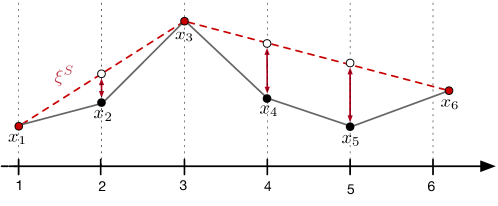
Figure 1: Illustration example of the $L_{1}^{S}$ function, with $S={1,3,6}$. The solid black curve connects the data point ${\bf{x}}$, the dashed red curve denotes the function $\xi^{S}$, and the red arrows denote the distance between the points in ${\bf{x}}$ and the function $\xi^{S}$. The $L_{1}^{S}({\bf{D}})$ value is the sum of these distances.

Figure 1 provides an example with a graphical illustration of the $L_{1}^{S}$ function. The black solid curve delineate ${\bf{x}}$. The set $S=(1,3,6)$ and the sampled points $x_{1},x_{3}$, and $x_{6}$ are colored red. $\xi^{S}$ is the piecewise linear function passing through the sampled points and is represented with dashed red lines. The red arrows denote the distance between the points in ${\bf{x}}$ and their corresponding values in $\xi^{S}$ and the $L_{1}^{S}$-score for the set $S$ is the sum of these distances. The procedure assumes that the first and the last points of ${\bf{x}}$ are in $S$.

Intuitively, the set of $k$ points that minimizes $\eqref{eq:auc_score}$ produce the minimal reconstruction error when linear interpolation is used as a reconstruction procedure. However, finding the set of $k$ points minimizing the $L_{1}$-scoring function may be computationally expensive. Hence this paper presents a differentially-private greedy algorithm that approximates (4). The sampling procedure is depicted in Algorithm 3 and is an instantiation of the SVT mechanism where the queries compute the $L_{1}$-scores of the potential interpolation steps.

input : ${\bf{x}}$: the data stream seen in the current $w$-period

$k$: the number of samples

$\epsilon_{s}$: the privacy budget

$\theta$: a threshold

output : $S$: A sample set of $k$ points in $[w]$

1

2$S=\{1\}$;  $t_{p}=1$

3 $\rho=\text{Lap}(2\Delta_{L}/\epsilon_{s})$

4 for $i=2\ldots,w$ do

5       $\mu_{i}=\text{Lap}(4k\Delta_{L}/\epsilon_{s})$

6       if $L_{1}^{[t_{p},i]}({\bf{x}})+\mu_{i}\geq\theta+\rho$ then

7             $S=S\cup\{i\}$

8             $t_{p}=i$

9      if $w-i\leq k-|S|$ then

10             $S=S\cup\{j\ \mid\ i<i\leq w\}$

11            

12      Break if $|S|=k$

return $S$

Algorithm 3 Sample - Adaptive AUC-based sampler

The mechanism takes, as inputs, the data stream ${\bf{x}}$ processed for the current $w$-period, the number of points $k$ to sample for measurements, along with the privacy budget $\epsilon_{s}$ and a user defined threshold $\theta\geq 0$ which influences the acceptable $L_{1}$-score for choosing the next point to sample. The values choice for $\theta$ in our application of interest are detailed in Section 6. Line (1) initializes the set of sample points $S$ with the first element of the $w$-period (this choice is necessary for executing the interpolation in the next steps), and it tracks the last point $t_{p}$ selected for sampling. The algorithm first generates the noise $\rho$ (line 2) for the threshold $\theta$ (line 5). For all but the first time step, the algorithm adds Laplace noise with parameter $4k\Delta_{L}/\epsilon$ to the $L_{1}^{[t_{p},i]}$-query (line 4), where $\Delta_{L}$ is the largest sensitivity associated with any of the $L_{1}$ scoring functions invoked by the algorithm (see Theorem 6). If the result is above the threshold, then point $i$ is added to $S$ (line 6) and the last selected point $t_{p}$ is updated (line 7). The mechanism keeps track of the number of index points already stored. It stops when the size of $S$ matches $k$ (line 10). The mechanism also tests if there are enough points to reach $k$ (line 8) and adds the remaining points if needed (line 9).

To run the mechanism, it is necessary to determine the sensitivity $\Delta_{L_{1}}^{[a,b]}$ of the $L_{1}$-score defined in (3), i.e.,

$$\Delta_{L_{1}}^{[a,b]}=\displaystyle\max_{{\bf{D}}\sim_{w}{\bf{D}}^{\prime}}\left|L_{1}^{[a,b]}({\bf{D}}^{\prime})-L_{1}^{[a,b]}({\bf{D}})\right|$$

where ${\bf{D}}$ and ${\bf{D}}^{\prime}$ are two w-neighboring data streams in a $w$-period.

The following theorem shows that $\Delta_{L_{1}}^{[a,b]}$ can be bounded, yielding a procedure to privately sample $k$ points in the $w$-period using an efficient, suboptimal, version of Equation (4).

Theorem​ 6

For an arbitrary $w$-period and fixed indexes $a,b\in[w]$ with $a<b$, the sensitivity $\Delta_{L_{1}}^{[a,b]}$ of the $L_{1}^{[a,b]}$ score is bounded by $2(b-a)$.

Proof. Consider two data stream $w$-periods ${\bf{D}}$ and ${\bf{D}}^{\prime}$ such that ${\bf{D}}\sim_{w}{\bf{D}}^{\prime}$ and focus, without loss of generality, on their associated stream counts ${\bf{x}}$ and ${\bf{x}}^{\prime}$. Let $\xi$ and $\xi^{\prime}$ be shorthands for $\xi^{[a,b]}$ and $\xi^{\prime[a,b]}$. The goal is to bound

$$\left|L_{1}^{[a,b]}({\bf{D}}^{\prime})-L_{1}^{[a,b]}({\bf{D}})\right|=\sum_{i=1}^{b}\left||\xi^{\prime}(i)-x^{\prime}_{i}|-|\xi(i)-x_{i}|\right|,$$

and each term of the summation can be bounded independently. If $i=a\,\lor\,i=b$, then $\xi^{\prime}(i)=x^{\prime}_{i}$ and $\xi(i)=x_{i}$, since $x^{\prime}_{i}$ and $x_{i}$ are interpolated exactly and $\displaystyle\left||\xi^{\prime}(i)-x^{\prime}_{i}|-|\xi(i)-x_{i}|\right|=0.$ Otherwise, note that $|x^{\prime}_{i}-x_{i}|\leq 1$ since $D_{i}\sim D^{\prime}_{i}=1$ for all $i\in[w]$ by definition of $w$-event privacy. Moreover, since the pairs ($\xi(a),\xi^{\prime}(a))$ and $(\xi(b),\xi^{\prime}(b))$ differ by at most 1, it follows that $|\xi^{\prime}(i)-\xi(i)|\leq 1$ for every point $i\in[a,b]$. There are four cases to consider.

(1) If $\xi^{\prime}(i)\geq x^{\prime}_{i}$ and $\xi(i)\geq x_{i}$, then

$$\left||\xi^{\prime}(i)-x^{\prime}_{i}|-|\xi(i)-x_{i}|\right| =\left|(\xi^{\prime}(i)-x^{\prime}_{i})-(\xi(i)-x_{i})\right|$$

$$=\left|(\xi^{\prime}(i)-\xi(i))-(x^{\prime}_{i}-x_{i})\right|$$

$$\leq 2.$$

(2) The case $\xi^{\prime}(i)<x^{\prime}_{i}$ and $\xi(i)<x_{i}$ is symmetric. (3) The case $\xi^{\prime}(i)\geq x^{\prime}_{i}$ and $\xi(i)<x_{i}$ requires a further case analysis.

• If $\xi^{\prime}(i)\leq\xi(i)$, we have $x^{\prime}_{i}\leq\xi^{\prime}(i)\leq\xi(i)<x_{i}$. Since $|x_{i}-x^{\prime}_{i}|\leq 1$, it follows that $|\xi^{\prime}(i)-x^{\prime}_{i}|\leq 1$ and $|\xi(i)-x_{i}|\leq 1$. Therefore

  $$\left||\xi^{\prime}(i)-x^{\prime}_{i}|-|\xi(i)-x_{i}|\right|\leq 1.$$

• If $\xi^{\prime}(i)>\xi(i)$, then $\xi(i)+1\geq\xi^{\prime}(i)>\xi(i)$, since $|\xi(i)-\xi^{\prime}(i)|\leq 1$. It follows that

  $$x^{\prime}_{i}\leq\xi^{\prime}(i)\leq\xi(i)+1<x_{i}+1.$$

  Since $|x_{i}-x^{\prime}_{i}|\leq 1$ and $|\xi(i)-\xi^{\prime}(i)|\leq 1$, $|\xi^{\prime}(i)-x^{\prime}_{i}|\leq 1$ and $|\xi(i)-x_{i}|\leq 1$ and therefore

  $$\left||\xi^{\prime}(i)-x^{\prime}_{i}|-|\xi(i)-x_{i}|\right|\leq 1.$$

(4) Finally, the last case, $\xi^{\prime}(i)<x^{\prime}_{i}$ and $\xi(i)\geq x_{i}$, is symmetric to previous one. Therefore

$$\Delta_{L_{1}}^{[a,b]}=\max_{{\bf{x}}\sim_{w}{\bf{x}}^{\prime}}|L_{1}^{[a,b]}({\bf{D}}^{\prime})-L_{1}^{[a,b]}({\bf{D}})|\leq 2(b-a).$$

$\Box$

Let $S=(\iota_{1},\ldots,\iota_{k})$ be a sequence of $k$ indexes in $[w]$. Because of the stopping criteria, the largest contiguous interval $[\iota_{i},\iota_{j}]$ for $i,j\in[k]$ has size $w-k$. The sensitivity of the $L_{1}$-score on such an interval is bounded by $2(w-k)$. Algorithm 3 thus uses

$$\Delta_{L}=2(w-k).$$

Theorem​ 7

Algorithm 3 is $\epsilon_{s}$-differential private.

Proof. The proof is a direct consequence of the correctness of the SVT mechanism (?), Theorem 6, and the definition of $\Delta_{L}$. $\Box$

3.2 The Perturbation Procedure

Given the set $S$ of $k$ sampling indexes for a $w$-period, the perturbation process takes as input the $k$-ary vector of the data stream measurements ${\bf{x}}[S]$ and outputs a noisy version $\tilde{{\bf{x}}}_{S}$ of such vector satisfying $\epsilon_{p}$-differential privacy. The process simply applies the Laplace mechanism with parameter $k\Delta_{A}/\epsilon_{p}$, where $\Delta_{A}$ is the sensitivity of the aggregation query.

Theorem​ 8

Perturb satisfy $\epsilon_{p}$-differential privacy.

The above result follows by straightforward application of the Laplace mechanism (Theorem 4) on a set of $k$ points and parallel composition (Theorem 2).

3.3 The Reconstruction Procedure

The Reconstruct procedure takes as input the noisy measurements $\tilde{{\bf{x}}}_{S}\in\mathbb{R}^{k}$ at the sample points $S$ in ${\bf{x}}$ and outputs a vector $\tilde{{\bf{x}}}\in\mathbb{R}^{w}$ of private estimates for the sub-stream ${\bf{x}}$. Each value $\tilde{x}_{i}$ of $\tilde{{\bf{x}}}$ is obtained evaluating the function $\xi^{S}$ at $i$. Section 4 analyzes how well the polynomial approximates the data stream at any point $x_{i}$. The reconstruction procedure is not required to query the real data stream and uses exclusively private information to compute its output. Hence, the output $\tilde{{\bf{x}}}$ remains $\epsilon_{s}+\epsilon_{p}$-differential private by post-processing immunity of differential privacy (Theorem 3).

3.4 The Optimization-based Post-Processing

13

input :  $\tilde{{\bf{x}}}$: the private data stream seen in the current $w$-period

$Q_{{\bf{F}}}({\bf{D}})$; the set of feature queries

$\epsilon_{o}$: the privacy budget

output : $\hat{{\bf{x}}}$: a private post-processed data stream

1

2${\bf c}=\mathcal{M}_{\mathrm{Lap}}({\bf{x}};Q_{{\bf{F}}_{i}},\epsilon/(p-1))$

3 ${\bf x}^{*}={\bf argmin}_{\bf\dot{x}}\|{\bf\dot{x}}-\tilde{{\bf{c}}}\|_{2,\lambda}^{2}=$

$$\sum_{i=1}^{p}\frac{1}{m_{i}}\sum_{j=1}^{m_{i}}(\dot{x}_{ij}-\tilde{c}_{ij})^{2}\;$$ (O1)

subject to $$:$$

$$\forall i^{\prime},i:{\bf{F}}_{i^{\prime}}\prec{\bf{F}}_{i},~{}~{}~{}j\in[m_{i}]:\dot{x}_{ij}=\sum_{l:{\bf{d}}_{i^{\prime}l}\subseteq{\bf{d}}_{ij}}\dot{x}_{i^{\prime}l}$$ (O2)

$$\forall i,j:\dot{x}_{ij}\geq 0.$$ (O3)

return $\hat{{\bf{x}}}=\dot{x}_{11},\ldots,\dot{x}_{1w}$

Algorithm 4 PostProcess – Optimization-based post-processing

The noise introduced in the previous steps may substantially alter the values of the elements in the w-period, so that some global properties of interest, such as the total sum of elements in the w-period may differ from its original value. The goal of the post-processing step is to redistribute the noise introduced by the previous steps using noisy information on aggregated values of the w-period. It does so by casting the noise redistribution as an optimization problem whose solution guarantees the consistency of different estimates of identical quantities.

The Post-process step computes the final estimates $\hat{{\bf{x}}}$ of the $w$-period data ${\bf{x}}$ using the private data $\tilde{{\bf{x}}}$ and additional queries over ${\bf{x}}$. The procedure is summarized in Algorithm 4. It uses the concept of features to capture semantic properties of the application of interest and queries these features in addition to using the noisy input $\tilde{{\bf{x}}}$ of the original data stream. For example, two important features in the analysis of WiFi connections profiles are those periods when peaks typically occur, as well as the total amount of connections occurring in an $w$-period.

Formally, a feature is a partition of the $w$-period and the size of the feature is the number of elements in the partition. We say that a feature ${\bf{F}}^{\prime}$ is a sub-feature of ${\bf{F}}$, denoted by ${\bf{F}}^{\prime}\prec{\bf{F}}$, if ${\bf{F}}^{\prime}$ is obtained by sub-partitioning ${\bf{F}}$. The feature query $Q_{{\bf{F}}}({\bf{D}})$ on data stream ${\bf{D}}$ associated with feature ${\bf{F}}=\{{\bf{d}}_{1},\ldots,{\bf{d}}_{m}\}$ returns an $m$-dimensional vector $(c_{1},\ldots,c_{m})$ where each $c_{i}$ is the sum of the values $x_{j}$ of ${\bf{x}}$ for $j\in{\bf{d}}_{i}$.

Example​ 3

Consider a w-period ${\bf{x}}\!=\!(10,15,20,23,41,72,55,50,88,72,40,18)$ of size 12 reporting the number of WiFi connections to an access point in a day-period. Consider a feature ${\bf{F}}_{1}=\{1,\ldots,12\}$ that includes the indexes for all the elements of the w-period. The associated feature query $Q_{{\bf{F}}_{1}}({\bf{D}})=(10,15,20,23,41,72,55,50,88,72,40,18)$ returns each frequency value observed during the day. Next, we consider a sub-feature ${\bf{F}}_{2}$ of ${\bf{F}}_{1}$, defined as ${\bf{F}}_{2}=\{\{1,2,3,4\},\{5,6,7,8,9\},\{10,11,12\}\}$. Its associated feature query $Q_{{\bf{F}}_{2}}({\bf{D}})=(68,306,130)$ describes the sums of all connection frequencies associated with time steps in $\{1,2,3,4\}$, $\{5,6,7,8,9\}$, and $\{10,11,12\}$, representing morning, afternoon, and evening hours respectively.

The optimization-based post-processing takes as input the noisy data stream $\hat{{\bf{x}}}$ from the reconstruction procedure and a collection of features queries $Q_{{\bf{F}}}({\bf{D}})$ for each ${\bf{F}}$ in the set of features ${\mathscr{F}}=\{{\bf{F}}_{1},\ldots,{\bf{F}}_{p}\}$. For notational simplicity, we assume that the first feature always partitions the data stream $w$-period into singletons, i.e., ${\bf{F}}_{1}=\{\{i\}:i\in[w]\}$. The noisy answer to this query is the output $\tilde{{\bf{x}}}$ of the perturbation procedure (line (2) of Algorithm 2). When viewed as queries, the inputs to the mechanism can be represented as a set of values $Q_{{\bf{F}}_{i}}({\bf{D}})={\bf c}_{i}=(c_{i1},\ldots,c_{im_{i}})$ $(1\leq i\leq p)$ or, more concisely, as ${\bf{c}}=(c_{11},\ldots,c_{pm_{p}})$. Finally, we assume that the partial ordering $\prec$ of features is given.

This first step of Algorithm 4 (line 1) applies the Laplace mechanism with privacy parameter $\frac{\epsilon}{p-1}$ to each feature query (excluding the first one whose answer $\tilde{{\bf{x}}}$ is already private), i.e.,

$$\mathcal{M}_{\mathrm{Lap}}({\bf{x}};Q_{{\bf{F}}_{i}},\epsilon/{p-1})=\tilde{c}_{i}=(\tilde{c}_{i1},\ldots,\tilde{c}_{im_{i}})\;\;\;(2\leq i\leq p).$$

The resulting values $\tilde{{\bf{c}}}=(\tilde{c}_{11},\ldots,\tilde{c}_{pm_{p}})$ are then post-processed by the optimization algorithm depicted in line (2) to obtain the values ${\bf{x}}^{*}=(x^{*}_{11},\ldots,x^{*}_{p{m_{p}}})$. Finally, the mechanism outputs a data stream $\hat{{\bf{x}}}=(\dot{x}^{*}_{11},\ldots,\dot{x}^{*}_{1w})$.

The essence of Algorithm 4 is the optimization model depicted in line (2). Its decision variables are the post-processed values $\dot{{\bf{x}}}=(\dot{x}_{11},\ldots,\dot{x}_{p{m_{p}}})$, and ${\bf\lambda}=(\lambda_{1},\ldots,\lambda_{p})\in(0,1]^{p}$ is a vector of reals representing weights for the terms of the objective function. The objective minimizes the squared weighted L₂-Norm of $\dot{{\bf{x}}}-\tilde{{\bf{c}}}$, where the weight $\lambda_{i}$ of element $x_{ij}-\tilde{c}_{ij}$ is $\frac{1}{m_{i}}$.

The optimization is subject to a set of consistency constraints among comparable features and non-negativity constraints on the variables. For each pair of features $({\bf{F}}_{i^{\prime}},{\bf{F}}_{i})$ with ${\bf{F}}_{i^{\prime}}\prec{\bf{F}}_{i}$, constraint O2 selects an element ${\bf{d}}_{ij}\in{\bf{F}}_{i}$ and all its subsets ${\bf{d}}_{i^{\prime}l}\in{\bf{F}}_{i^{\prime}}$ and imposes the constraint

$$\dot{x}_{ij}=\sum_{l:{\bf{d}}_{i^{\prime}l}\subseteq{\bf{d}}_{ij}}\dot{x}_{i^{\prime}l},$$

which ensures that the post-processed value $\dot{x}_{ij}$ is consistent with the sum of the post-processed values of its partition in ${\bf{F}}_{i^{\prime}}$. By definition of sub-features, there exists a set of elements in ${\bf{F}}_{i^{\prime}}$ whose union is equal to ${\bf{d}}_{ij}$.

Theorem​ 9

The optimization-based post-process achieves $\epsilon_{o}$-differential privacy.

Proof. Since each feature partitions the $w$-period over the data stream, each feature query is a count query with sensitivity 1. Thus, each $\tilde{c}_{ij}$ $(i>1)$ obtained from the Laplace mechanism is $\epsilon_{o}$-differential-private by Theorem 4 and the values $\tilde{{\bf{x}}}=\tilde{c}_{11},\ldots,\tilde{c}_{1w}$ are differential private (Theorems 7 and 8). Additionally, $(\tilde{c}_{11},\ldots,\tilde{c}_{pm_{p}})$ is $\epsilon_{o}$-differential-private by Theorem 1. Finally, the result follows from post-processing immunity (Theorem 3). $\Box$

Observe that the mechanisms considered in this paper all operate over the universe of the data stream in the $w$-period. This is the case for instance of the Laplace mechanisms which runs in polynomial time in the size of the $w$-period. The next theoretical result characterizes the complexity of the optimization model depicted in line (2) and hence the complexity of Algorithm 4. Recall that a $\delta$-solution to an optimization problem is a solution whose objective value is within distance $\delta$ of the optimum.

Theorem​ 10

A $\delta$-solution to the optimization to the optimization model in line (2) (Algorithm 4) can be obtained in time polynomial in $w$, the number of features, and $\frac{1}{\delta}$.

Proof. First observe that the number of variables and constraints in the optimization model are bounded by a polynomial in size of the period $w$ and the number of features $p$. Indeed, since the features are partitions, every set ${\bf{d}}_{i^{\prime}l}$ in Constraint (O2) is a subset of exactly one ${\bf{d}}_{ij}$. The result then follows from the fact that the optimization model is convex, which implies that a $\delta$-solution can be found in time polynomial in the size of the universe, the number of features, and $\frac{1}{\delta}$ (?). $\Box$

4 Error analysis

This section analyzes how the sampling and reconstruction procedure can improve the accuracy of the output. It characterizes the error $\mathbb{E}\|\hat{{\bf{x}}}-{\bf{x}}\|_{2}^{2}$ of the results of Algorithm 2 over a $w$-period stream release, when the equally-spaced approach is selected as a sampling procedure and no post-processing is applied (i.e., when the algorithm releases $\tilde{{\bf{x}}}$ (line 2, Algorithm 2)).

4.1 Sample and Reconstruct

Consider a $w$-period of the data stream ${\bf{x}}$ using the same notational assumptions introduced in the previous period, and thus we focus in a $w$-period in $[1,w]$. Let $k=|S|$ be the number of samples selected for measurements, by the equally-spaced sampling in addition to the initial point. This determines the length of each segment $m=w/k$ during which the Reconstruct procedure interpolates values without extra measurements. We assume $m$ to be an even integer. Let $L$ be the Lipschitz constant defined as $L:=\sup_{t\in[w]}x_{t}-x_{t-1}$.

Theorem​ 11

The error introduced by Algorithm 2 (ignoring post-processing) with the equally-spaced sampling procedure with parameter $k$ is bounded by $O\left(m^{2}L^{2}w+2\frac{w^{2}L}{\epsilon}+\frac{w^{3}}{m^{2}\epsilon^{2}}\right)$.

Proof. For notational simplicity, consider the first interval $I=\{1,\ldots,m\}$ of the $w$-period, where the sample points $1$ and $m$ are selected. Thus, $x_{1}$ and $x_{m}$ are measured privately. The reconstruct procedure uses linear interpolation between $x_{1}$ and $x_{m}$ to recover the values of the non-sampling points $x_{2},\ldots,x_{m-1}$.

For each point $i\in[m]$, there are two sources of error: the perturbation error $e_{p}$ and the reconstruction error $e_{r}$. The worst-case reconstruction error is bounded by $e_{r}=mL$. The perturbation error $e_{p}$ is the additive Laplace noise. There are $k$ measurements taken, and hence the privacy budget $\epsilon$ must be divided by $k$, which results in $e_{p}=|\tilde{x}_{i}-x_{i}|=\mathrm{Lap}(k/\epsilon)$. This error adds to the perturbation error at every point in the $w$-period. Therefore, for all $i\in[m]$, the expected error is:

$$\mathbb{E}\|\tilde{x}_{i}-x_{i}\|_{2}^{2} \leq\mathbb{E}\left[(e_{r}+e_{p})^{2}\right]$$

$$\leq\mathbb{E}_{Z\sim\mathrm{Lap}(k/\epsilon)}\left[(mL+Z)^{2}\right]$$

$$=m^{2}L^{2}+2mL\frac{k}{\epsilon}+(\frac{k}{\epsilon})^{2}.$$

Multiplying this quantity by the number $m$ of points in the interval gives

$$\mathbb{E}\|\tilde{{\bf{x}}}[I]-{\bf{x}}[I]\|_{2}^{2} \leq m\mathbb{E}\|\tilde{x}_{i}-x_{i}\|_{2}^{2}\leq m^{3}L^{2}+2m^{2}L\frac{k}{\epsilon}+m(\frac{k}{\epsilon})^{2}.$$

As a result, the error $\|\tilde{{\bf{x}}}[I]-{\bf{x}}[I]\|_{2}^{2}$ is bounded by $O(m^{3}L^{2}+2m^{2}L\frac{k}{\epsilon}+m(\frac{k}{\epsilon})^{2})$. Multiplying the above by the number of intervals $\frac{w}{m}$ in the $w$-period gives the final error which is bounded by

$$O\left(m^{2}L^{2}w+2\frac{w^{2}L}{\epsilon}+\frac{w^{3}}{m^{2}\epsilon^{2}}\right).$$

$\Box$

For $m=\sqrt{\frac{w}{\epsilon L}}$, the above expression generates an error of $O(w^{2}L/\epsilon)$. In comparison, applying the Laplace mechanism to produce a private sub-stream in the $w$-period produces an error of $w\,\mathbb{E}_{\mathrm{Lap}(w/\epsilon)}[Z^{2}]=\frac{w^{3}}{\epsilon^{2}}.$

The result above shows that choosing a sampling parameter $k$ to sample uniformly every $m$ time steps may allow Algorithm 2 to produce outputs with a substantially lower error than those obtained by the Laplace mechanism. Although this result applies to the equally-spaced sampling procedure, Section 6 demonstrates experimentally that the $L1$-sampling procedure outperforms its equally-spaced counterpart.

4.2 Optimization-based Post-Processing

The following result is from (?). It bounds the error of the optimization-based post-processing. It proves that the post-processing step can accommodate any side-constraints without degrading the accuracy of the mechanism significantly.

Theorem​ 12

The optimal solution to the optimization model in line (2) of Algorithm 2 satisfies

$$\|{\bf{x}}^{*}-{\bf{x}}\|_{2,\lambda}\leq 2\|\tilde{{\bf{x}}}-{\bf{x}}\|_{2,\lambda}.$$

Proof. It follows that:

$$\|{\bf{x}}^{*}-{\bf{x}}\|_{2,\lambda} \leq\|{\bf{x}}^{*}-\tilde{{\bf{x}}}\|_{2,\lambda}+\|\tilde{{\bf{x}}}-{\bf{x}}\|_{2,\lambda}$$

$$\leq 2\|{\bf{x}}-\tilde{{\bf{x}}}\|_{2,\lambda}.$$

where the first inequality follows from the triangle inequality on weighted L₂-norms and the second inequality follows from

$$\|{\bf{x}}^{*}-\tilde{{\bf{x}}}\|_{2,\lambda}\leq\|{\bf{x}}-\tilde{{\bf{x}}}\|_{2,\lambda}$$

by optimality of ${\bf{x}}^{*}$ and the fact that ${\bf{x}}$ is a feasible solution to constraints (O2) and (O3). $\Box$

5 Privacy Model Extensions

This section first presents an extension of the privacy model that protects disclosure of arbitrary quantities within the $w$-event privacy model. It then generalizes the theoretical results of OptStream to this extended privacy model. Finally, it describes an extension of OptStream that supports hierarchical data streams.

5.1 $\alpha$-Indistinguishability for Data Streams

The application studied in this paper requires the private release of energy load consumption streams. Unlike the previous setting, where the participation of users is revealed at each time step, the new privacy setting requires the load consumption of each customer to be revealed for each time steps. To capture this requirement, the data stream setting presented in Section 2.2 is extended to an infinite sequence of elements in the data universe ${\mathscr{U}}=\mathcal{I}\times\mathcal{R}\times\mathcal{T}$, where $\mathcal{I}$ and $\mathcal{T}$ are defined as in Section 2.2, and $\mathcal{R}$ is the set of possible events (i.e., the data items generated by users). In other words, each tuple $(i,r,t)$ describes an event that occurred at time $t$ in which user $i$ reported value $r$.

Each user transmits an aggregate summary of the stream periodically (e.g., every 30 minutes) and the discrete time step $k$ represents an aggregate (e.g., the sum or the average) of all values describing the event occurring in time period $k$. This setting implies that a tuple $(i,r,t)$ describes the aggregate behavior of user $i$ during the time period $t$. Here, a numerical count query $Q:\mathcal{D}\to\mathbb{R}^{|\mathcal{I}|}$ returns an $|\mathcal{I}|$-dimensional vector corresponding to the aggregated reports of each user in $\mathcal{I}$. The following example illustrates such behavior.

Example​ 4

Consider a data stream system that collects power consumption data from customers of an electric company distributed on a wide geographical region. Customers may correspond to facilities (such as homes, hospitals, industrial buildings) or electrical substations, transmitting their power consumption at regular intervals (e.g., every $30$ minutes). The value $r_{t}\in\mathcal{R}$ transmitted by a customer at time $t$ is a real number denoting the average amount of power (in MegaWatts) the customer required during time interval $t$. The table below represents a the scenario in which user $\text{customer}_{1}$ consumes $3.1$ MW at time $t=1$, $3.2$ MW at time $t=2$, and $2.8$ MW at time $t=3$.

$\mathcal{I}$	$Q(D_{1})$	$Q(D_{2})$	$Q(D_{3})$	…
$\text{customer}_{1}$	3.1	3.2	2.8
$\text{customer}_{2}$	1.0	1.5	1.6
$\text{customer}_{2}$	0.7	1.1	1.2

Customer identities are assumed to be a public information, as every facility consumes power. However, their load fluctuations are considered to be highly sensitive. Indeed. changes in power consumption may indirectly reveal production levels and hence strategic investments, decreases in sales, and other similar information. These changes should not be revealed within some application-specific period of $w$ time steps. Thus, within each $w$-period, the privacy goal of the data curator is to protect observed increases or decreases of power consumptions. More precisely, consider $r_{u}^{t}$ and ${r^{\prime}}_{u}^{t}$ be two distinct values that may be reported by user $u$ at time $t$ and that satisfy $|r_{u}^{t}-{r^{\prime}}_{u}^{t}|\leq\alpha$ for some positive real value $\alpha$. An attacker should not be able to confidently determine that $u$ reported value $r_{u}^{t}$ instead of value ${r^{\prime}}_{u}^{t}$ and vice-versa.

This goal can be achieved by using a more general adjacency relation between datasets. This relation needs to capture the distance between reported quantities whose magnitudes must be protected up to some given value $\alpha>0$. The value $\alpha$ is called the indistinguishability level. This generalized definition of differential privacy has been adopted in several applications and has sound theoretical foundations (e.g., (?, ?, ?)). Consider a dataset $X$ to which $n$ individuals contribute their real-valued data $r_{i}\in\mathbb{R}$, i.e., $X=(r_{1},\ldots,r_{n})\in\mathbb{R}^{n}$. For $\alpha>0$, an adjacency relation that captures the indistinguishability of a single individual to the aggregating scheme is:

$$X\sim_{\alpha}X^{\prime}\;\Leftrightarrow\;\exists i\textrm{~{}s.t.~{}}|r_{i}-r^{\prime}_{i}|\leq\alpha\textrm{~{}and~{}}r_{j}=r^{\prime}_{j},\forall j\neq i.$$ (5)

Such adjacency definition, in our target domain, is useful to hide increases or decreases of loads up to some quantity $\alpha$. The generalization of differential privacy that uses the above adjacency relation is referred to as $\alpha$-indistinguishability (?).

The $w$-privacy definition, introduced in Definition 2, can be extended to use $\alpha$-indistinguishability by replacing the standard neighboring relation between datasets with the adjacency relation defined in Equation (5). More precisely, for a given $\alpha>0$, two data streams prefixes $D[t],D^{\prime}[t]$ are said ($w,\alpha$)-neighbors, written $D[t]\sim_{w}^{\alpha}D^{\prime}[t]$, if (i) for each $D_{i},D_{i}^{\prime}$ with $i\in[t]$, $D_{i}\sim_{\alpha}D_{i}^{\prime}$, and (ii) for each $D_{i},D_{i}^{\prime},D_{j},D_{j}^{\prime}$, with $i<j\in[t]$ and $D_{i}\neq D_{i}^{\prime},D_{j}\neq D_{j}^{\prime}$, it must be the case that $j-i+1\leq w$ holds.

Definition​ 3 (($w,\alpha$)-indistinguishability)

Let $\mathcal{A}$ be a randomized algorithm that takes as input a stream prefix $D[t]$ of arbitrary size and outputs an element from a set of possible output sequences ${\mathcal{O}}$. $\mathcal{A}$ satisfies $w$-event $\epsilon$-differential privacy under $\alpha$-indistinguishability ($(w,\alpha$)-indistinguishability for short) if, for all sets $O\subseteq{\mathcal{O}}$, all $(w,\alpha)$-neighboring stream prefixes $D[t],D^{\prime}[t]$, and all $t$:

$$\frac{Pr[\mathcal{A}(D[t])\in O]}{Pr[\mathcal{A}(D^{\prime}[t])\in O]}\leq\exp(\epsilon).$$ (6)

This privacy definition combines $w$-event privacy (?) and a metric-based generalization of differential privacy (?) in order to meet the requirements of the motivating application. Notice that ($w,\alpha$)-indistinguishability is a generalization of $w$-privacy, and it reduces to $w$-privacy when $\alpha=1$.

OptStream can be naturally extended to satisfy this definition, by calibrating the noise introduced by the Laplace mechanism, used during the sampling (Theorem 6), perturbation (Theorem 8), and post-processing (Theorem 9) steps, to satisfy the above definition. More practically, it is achieved by updating the definition of query sensitivity as:

$$\Delta_{Q}=\max_{D[t]\sim_{w}^{\alpha}D^{\prime}[t]}\|Q(D[t])-Q(D^{\prime}[t])\|_{1}.$$

Thus, in the ($w,\alpha$)-indistinguishability model, the sensitivity of each query $Q$ used during the perturb (see Section 3.2) and the post-process (see Section 3.4) procedures is $\Delta_{Q}=\alpha$, and the sensitivity $\Delta_{L}$ of of the queries adopted in the $L1$-based reconstruction procedure (see Section 3.3) is $\Delta_{L}=2\alpha(w-k)$ . The behavior of OptStream for different indistinguishability levels is presented in Section 6.

5.2 Hierarchical Data Streams

OptStream can also be generalized to support hierarchical data streams. A data stream $D$ is called hierarchical if, for any time $t$, there is an aggregation entry $a=(i_{a},r_{a},t)$ associated with an aggregation set $S_{a}\subseteq\mathcal{I}$ that reports the sum of values reported by all entries in $S_{a}$ at time $t$, i.e., $r_{a}=\sum_{u\in S_{a}}r_{u}^{t}$. More formally, a data stream is hierarchical if, for any two aggregation entries $a_{1},a_{2}$, either $S_{a_{1}}\subset S_{a_{2}}$ or $S_{a_{2}}\subset S_{a_{1}}$ holds or $S_{a_{1}}\cap S_{a_{2}}=\emptyset$ is true.

A set of aggregation entries $\mathcal{S}$ can be represented hierarchically through a tree (called an aggregation tree) in which the root is defined by the entry that is not contained in any other entries and the children of an aggregation entry $p$ are all the entries in $D$ whose identifiers are contained in $S_{p}$. The height of a hierarchical data is the maximum path length from the root to any leaf of its tree.

Example​ 5

In our target application, a data curator is interested in the aggregated load consumption stream at the level of a small geographical region, at a group of regions within the same electrical sub-station, and finally at the nation-level. These aggregations form a hierarchy whose root is represented by the nation-level aggregation entry, its children by the electrical sub-station entries, and the tree leaves by the region-level entries.

To answer each query of the hierarchical stream, OptStream is extended as follows. For each $w$-period, the algorithm runs the sampling, perturbation, and reconstruction procedure for each level of the aggregation tree representing the hierarchical stream. Finally, the post-processing optimization takes as input the answers to all the aggregation entries queries with the set of features being equal to the set of aggregation entries. The post-processing step thus enforces consistency between the aggregation counts at a node and the sum of counts at its children nodes in the tree, in addition to the features described earlier in the paper.

Theorem​ 13

For a hierarchy of height $h$, OptStream, when using a privacy budget of $\epsilon/h$ for each level of the hierarchy, satisfies $\epsilon$-differential privacy.

The result follows from the privacy guarantee of OptStream (Theorem 1), parallel composition of differential privacy across each level of the hierarchy (Theorem 2), and sequential composition of differential privacy, for each of the $h$ hierarchical queries (Theorem 1).

6 Evaluation

This section evaluates OptStream on real data streams for a number of tasks. It first evaluates the accuracy of the private release of a stream of data within the $w$-privacy model. Then, it studies the accuracy of each of the four individual components of the algorithm. Finally, it evaluates the algorithm within the ($w,\alpha$)-indistinguishability model.

Dataset

The source data was obtained through a collaboration with Réseau de Transport d’Électricité, the largest energy transmission system operator in Europe. It consists of a one-year national-level load energy consumption data with a granularity of 30 minutes. The data is aggregated at a regional level and ${\mathscr{R}}$ denotes the set of regions. Each data point in the stream represents the total load consumption of the customers served within a region during a 30 minute time period. Thus, for every region $R\in{\mathscr{R}}$, a stream of data ${\bf{x}}(R)=x_{1}(R),x_{2}(R),\ldots$ is generated where $x_{t}(R)$ represents the energy demand to supply in order to serve the region $R$ at time $t$. When the streams of all regions are aggregated, the resulting load consumption data constitutes a data stream of the energy profile at a national level.

For evaluation purposes, the experiments often consider a representative region (Auvergne - Rhône-Alpes) to analyze the data stream release. For the evaluation of hierarchical data streams, the experiments consider a hierarchical aggregation tree of height $2$, where the root node is the national level and each of the leaves corresponds to one region. Table 2 lists an overview of the data streams derived from the real energy load consumption data for each French region in 2016. Each data stream contains 17,520 entires.

Stream Data Regions (${\mathscr{R}}$)	Daily Average (MW)		Stream Data Regions (${\mathscr{R}}$)	Daily Average (MW)
Auvergne-Rhône-Alpes	7717.58		Ile de France (Paris)	8315.13
Bretagne	2554.23		Nouvelle Aquitaine	4985.68
Bourgogne - Franche-Comtè	2498.23		Normandie	3267.22
Centre - Val de Loire	2157.97		Occitanie	4314.7
Grand Est	5286.24		Pays de la Loire	3174.17
Hauts de France	5832.26		Provence - Cote d’Azur	4782.4

Table 2: Overview of the power load consumption stream data derived from the France regions in 2016. Daily Average refers to the average power (in MW) demanded daily. The number of time steps available for all regions is 17,520.

Algorithms

The following sections evaluate two versions of OptStream, with equally-spaced sampling and with the $L1$-sampling. They are compared against the Laplace mechanism and the Discrete Fourier Transform (DFT) algorithm (?). All the algorithms release private data associated with the sub-streams ${\bf{x}}$ for each $w$-period.

To ensure $\epsilon$-differential privacy for each $w$-period, the Laplace mechanism applies Laplace noise with parameter $\epsilon/w$ to each value in the period. To ensure $\epsilon$-differential privacy, the DFT algorithm works as follows. For each $w$-period, and given a value $k<w$, it first computes the Fourier coefficients $DFT({\bf{x}})_{j}=\sum_{i=1}^{w}\exp(\frac{2\pi\sqrt{-1}}{w}jix_{i})$ of each sub-stream ${\bf{x}}$ and each $j\in[w]$. It then considers the $k$ coefficients of lowest frequencies – which represent the high-level trends in ${\bf{x}}$ – and perturbs them using Laplace noise with parameter $\sqrt{k}\Delta_{2Q}/\epsilon$, where $\Delta_{2Q}$ is the $L_{2}$ sensitivity of the count query. It then pads the vector of noisy coefficients with a $(w-k)$-dimensional vector of $0$’s to obtain a $w$-dimensional vector. Finally, it applies the Inverse Discrete Fourier Transform (IDFT) to this $w$-dimensional vector to obtain a noisy estimate of the elements in the $w-$period. In more details, if $\hat{f}_{j}$ is the j-th perturbed coefficient of the series, the noisy estimate for the value $x_{j}$ is obtained through the IDFT function as: $\frac{1}{w}\sum_{i=1}^{w}\exp(\frac{2\pi\sqrt{-1}}{w}ji)\hat{f}_{j}$.

6.1 Stream Data-Release in the $w$-Privacy Model

This section evaluates the accuracy of privately releasing a data stream within the $w$-privacy model. It first studies the prediction error of the algorithms. It then analyzes the accuracy of privately releasing hierarchical streams on aggregated queries. Finally, it analyzes the accuracy of forecasting tasks from the released private data streams.

Real                            Laplace                            DFT                        OptStream

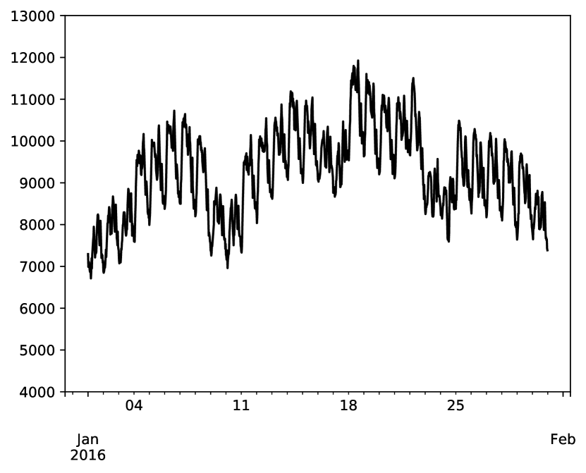
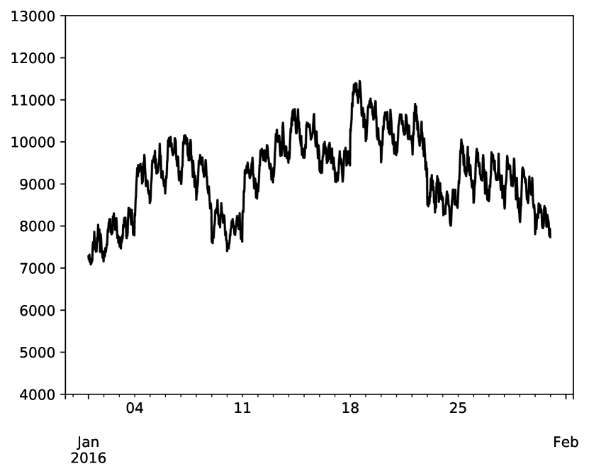
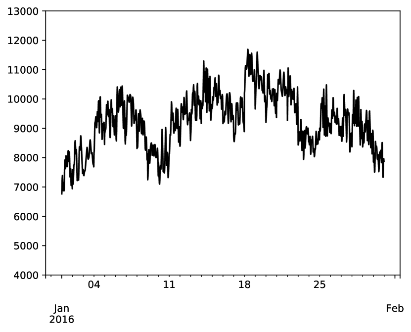
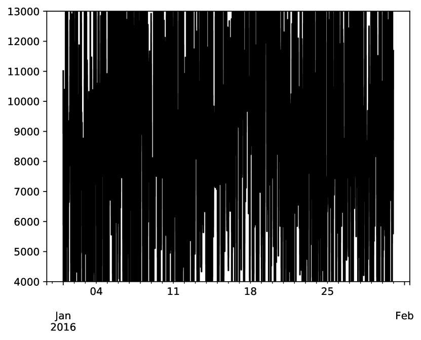
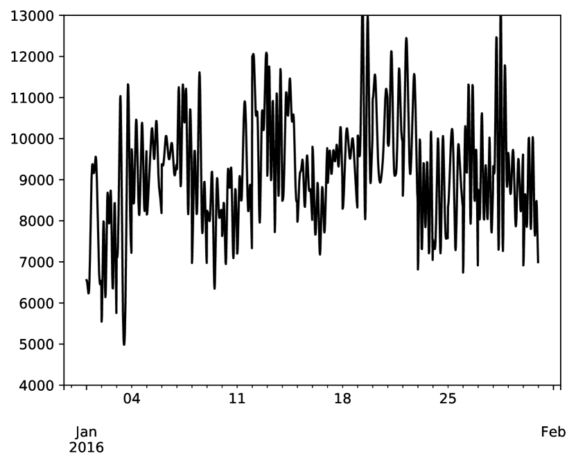
Figure 2: Real load consumption data for the Auvergne-Rhône-Alpes region in January 2016 (first column) and its private versions obtained using Laplace (second column), DFT (third column), and OptStream (fourth column) with privacy budget $\epsilon=1$ (top), $\epsilon=0.1$ (middle), and $\epsilon=0.01$ (bottom).

Answering queries over contiguous $w$-periods corresponds to releasing the private stream over the entire available duration. Figure 2 illustrates the real and private versions of the data-stream for the Auvergne-Rhône-Alpes region in January, 2016. It uses $w$-periods of size 48 for given privacy budgets $\epsilon=1.0$, $0.1$, and $0.01$, shown in the top, middle, and bottom rows respectively. Recall that the choice for the $w$-period allows the data curator to ensure the protection of the observed power consumptions within each period. Thus, the released stream protects loads in each entire day.

The real loads are illustrated in the first column. The figure compares our proposed OptStream algorithm (fourth column) against the Laplace mechanism (second column), and the DFT algorithm (?) (third column).

The experiments set the number of Fourier coefficients in the DFT and sampling steps in OptStream to $10$. The privacy budget allocated to perform each measurement is split equally. Additionally, for OptStream  $\epsilon_{s}=\epsilon_{p}=\epsilon_{o}=\frac{1}{3}\epsilon$, and the $L1$-sampling procedure uses a threshold value $\theta$ of $1000$ (which is about one tenth of the average load consumption in each region). This information was publicly revealed. Finally, OptStream uses the following feature query set ${\mathscr{F}}=\{{\bf{F}}_{1},{\bf{F}}_{2},{\bf{F}}_{3}\}$ in the optimization-based post processing step, with ${\bf{F}}_{1}\prec{\bf{F}}_{2}\prec{\bf{F}}_{3}$. ${\bf{F}}_{1}$ is defined as described in Section 3.4; ${\bf{F}}_{2}$ partitions each $w$-period in $4$ sets, the intervals $[0,14)$, $[14,24)$, $[24,36)$, and $[36,48)$ that correspond to aggregated consumption for the following times of the day: [0am-7am), [7am-12pm), [12pm-6pm), and [6pm-0am) respectively. ${\bf{F}}_{3}$ partitions each $w$-period in a single set, listing all the time steps within the $w$-period and thus describing the aggregated daily energy consumption. The query set represents salient moments in the day associated with different consumption patterns. These are proxy of consumer behaviors and thus energy consumption. Because these queries return private answers, the privacy is guaranteed by the post-processing immunity of DP (see Theorem 3). Finally, if an algorithm reports negative noisy value for a stream point, we truncate it to zero.

Figure 2 clearly illustrates that, for a given privacy disclosure level, OptStream produces private streams that are more accurate than its competitors when visualized. The next paragraph quantifies the error reported by the algorithms.

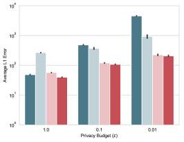
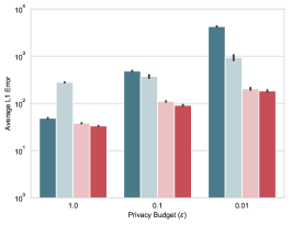
February     June     October                 

Figure 3: $L_{1}$-error analysis: Load stream data for the months of February (left), June (middle), and October (right). The $y$-axis reports $\log_{10}$ of the average $L_{1}$-error for all the stream data streams $R\in{\mathscr{R}}$.

6.1.1 Average $L_{1}$-Error Analysis

This section reports the average $L_{1}$-error for each $w$-period produced by the algorithms. For each input data stream ${\bf{x}}_{R}$ associated to a region $R\in{\mathscr{R}}$ (illustrated in Table 2) and each reported private stream $\hat{{\bf{x}}}_{R}$, we compare the average $L_{1}$-error defined as: $\frac{1}{N_{R}}\|\hat{{\bf{x}}}_{R}-{\bf{x}}_{R}\|_{1}$, where $N_{R}$ is the length of the data stream associated with region $R$. Figure 3 reports the average errors across all streaming regions $r\in{\mathscr{R}}$ for the months of February (left), June (middle), and October (right). The consumptions in these three months capture different customers load profile behaviors due to different weather patterns and durations of the day light. Each histogram reports the log₁₀ value of the average error of 30 random trials. Two version of OptStream (OptStreamES and OptStreamLS) are presented and correspond to the qqually-spaced sampling, and the $L1$-sampling procedures, respectively. While all algorithms induce a notable $L_{1}$-error which increases as the privacy budget decreases, the figure highlights that OptStream consistently outperforms competitor algorithms. Additionally, OptStream with $L1$-sampling is found to outperform its equally-spaced sampling counterpart, especially for large privacy budgets. For small privacy budgets, the two versions of the algorithm tend to perform similarly. This is due to the fact that the $L1$-score becomes less accurate as the amount of noise increases.

6.1.2 Hierarchical Private Data-Stream Release

This section evaluates the extensions proposed in Section 5.2 for releasing aggregated queries over hierarchical data streams. We answer the following queries over contiguous $w$-periods for the whole duration of the stream: count queries over the data stream ${\bf{x}}(R)=x_{1}(R),x_{2}(R),\ldots$ for each region $R\in{\mathscr{R}}$ listed in Table 2, as well as count queries ${\bf{x}}=x_{1},x_{2},\ldots$, where each $x_{t}=\sum_{R\in{\mathscr{R}}}x_{t}(R)$ represents the aggregated load consumption at national level. Thus, we create a hierarchy of two levels and answer simultaneously all queries. We allocate a privacy budget of $\frac{\epsilon}{2}$ to each level of the hierarchy. OptStream is compared against the Laplace mechanism applied to each stream data, using a uniform allocation of the privacy budget ($\frac{\epsilon}{2}$) for each query in a different level of the stream hierarchy and the DFT algorithm which answers queries over each data stream by uniformly allocating a portion of the privacy budget at each level of the hierarchy.

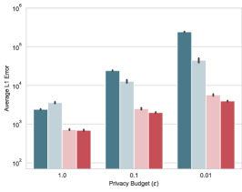
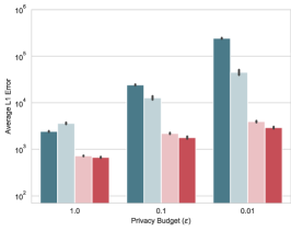
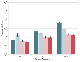
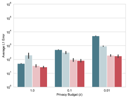
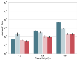
February     June     October                 

Figure 4: $L_{1}$-error analysis: Hierarchical energy load stream data for the months of February, June, and October. The $y$-axis reports $\log_{10}$ of the average $L_{1}$-error at national level (top) and at the regional level (bottom).

Figure 4 shows the results for three different months of the year: February (left), June (middle), and October (right), and under different indistinguishability parameters $\alpha$ for privacy budget $\epsilon=1.0$. The top row of the figure reports the average $L_{1}$-errors when releasing stream data ${\bf{x}}(R)$ associated with each region $R$, while the bottom row gives the $L_{1}$-errors when releasing the stream data ${\bf{x}}$ at national level. Each histogram reports the log₁₀ value of the average error of 30 random trials. The results illustrates similar trends to those in previous experiments. Overall, OptStream with the adaptive $L1$-sampling produces stream data with the lowest average $L_{1}$-errors for both levels of the stream hierarchy. In addition to the improved error it is important to note that OptStream ensures the consistency of the values of the private stream in the hierarchy, i.e., for each time step, the reported sum of the loads across all regions equals the reported load at national level. Neither the Laplace mechanism nor DFT do ensure such property.

6.1.3 Impact of Privacy on Forecasting Demand

The final results evaluate the capability of the released private streams to accurately predict future consumptions. To do so, we adopt the Autoregressive Moving Average (ARMA) model (?, ?, ?, ?). ARMA is a popular stochastic time series model used for predicting future points in a time series (forecast). It combines an Autoregressive (AR) model (?) and a Moving Average (MA) model (?, ?), i.e., ARMA($p,q$) combines AR($p$) and MA($q$) and is suitable for univariate time series modeling. In an AR($p$) model, the future value of a variable $x_{t}$ is assumed to be a linear combination of the past $p$ observations and a random error: $x_{t}=c+\sum_{i=1}^{p}\phi_{i}x_{t-i}+\beta_{t}$, where $c$ is constant, $\beta_{t}$ is a random variable modeling white noise at time $t$, and the $\phi_{i}(i=1,\ldots,p)$ are model parameters. A MA($q$) model uses the past $q$ errors in the time series as the explanatory variables. It estimates a variable $x_{t}$ using $\mu+\beta_{t}+\sum_{i=1}^{q}\theta_{i}\beta_{t-i}$, where the $\theta_{i}(i=1,\ldots,q)$ are model parameters, $\mu$ is the expectation of $x_{t}$, and the $\beta_{t}$ terms are white noise error terms. The ARMA model with parameters $p$ and $q$ refers to the model with $p$ autoregressive terms and $q$ moving-average terms: It estimates a future time step value $x_{t}$ as $c+\beta_{t}+\sum_{i=1}^{p}\phi_{i}x_{t-i}+\sum_{i=1}^{q}\theta_{i}\beta_{t-i}$. In our experiments, we use an ARMA model with parameters $p=q=1$ to estimate the future 48 time steps (corresponding to a day) when trained with the past four weeks of the private data stream estimated using Laplace, DFT, and OptStream with $L1$-sampling. All models use the same parameters adopted in the previous sections.

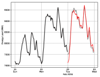
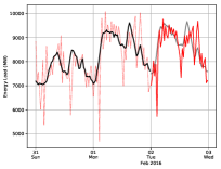
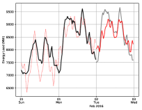
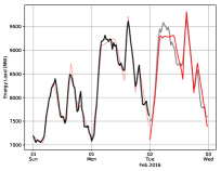
Real                            Laplace                            DFT                        OptStream

Figure 5: Prediction error: Forecast for a one day load consumption through an ARMA model on the real load consumption data (Real) and its private versions obtained using Laplace, DFT, and OptStream with privacy budget $\epsilon=0.1$.

Figure 5 visualizes the forecast for the load consumptions in the Auvergne-Rhône-Alpes region for February 2, 2016. The black and gray solid lines illustrates, respectively, the real load values observed so far and those of the day to be forecasted. The dotted red lines illustrates the private stream data estimated so far (and used as input to the prediction model) and the solid red lines depict the prediction obtained using the ARMA model. Figure 5 shows the forecast results using the real data (Real) and the private stream obtained through Laplace, DFT, and OptStream, respectively. The figure clearly shows that OptStream is able to visually produce better estimates for the next day forecast.

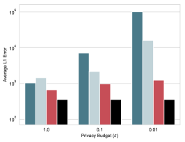
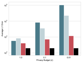
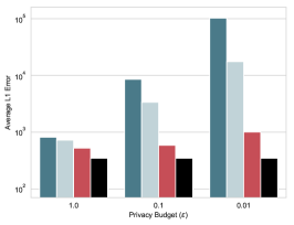
February     June     October                 

Figure 6: $L_{1}$ error analysis: ARMA forecasting model on stream data for the energy loads of the months of February, June, and October for the Auvergne-Rhône-Alpes region.

We also quantitatively evaluate the average $L_{1}$-error for each prediction produced by the mechanisms. We adopt the same setting as above for the prediction and report, in Figure 6, the average $L_{1}$-error for predicting each day in the month of February, June, and October for the Auvergne-Rhône-Alpes region. Each histogram reports the log₁₀ value of the average error of 30 random trials. We observe that OptStream reports the smallest errors compared to all other privacy-preserving algorithms, and that the error made by OptStream in reporting the next day forecast is closer to the error made in the forecast prediction using the real data than when using another method.

6.2 Evaluation of OptStream Individual Components

Real                         $\langle P,\circ,\circ\rangle$                     $\langle P,\circ,O\rangle$                   $\langle P,S,\circ\rangle$                     $\langle P,S,O\rangle$

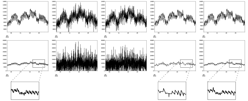
Figure 7: Real load consumption data for the Auvergne-Rhône-Alpes region in January, 2016 (Real) and OptStream activating: exclusively the perturbation step ($\langle P,\circ,\circ\rangle$), perturbation and optimization steps ($\langle P,\circ,O\rangle$), perturbation and sampling steps ($\langle P,S,\circ\rangle$), and all steps ($\langle P,S,O\rangle$ ). The top row, illustrates the results for privacy budget $\epsilon=0.1$, while the bottom row uses $\epsilon=0.01$. The boxes in the last two quadrants provide a zoom to illustrate in more details the reconstructed time series.

We also evaluate the effect of the sampling step as well as the benefits of the post-processing procedure of OptStream. Figure 7 visualizes the real (first column) and OptStream-based private version (other columns) load consumption data for the Auvergne-Rhône-Alpes region in January, 2016. The top row and bottom rows illustrate results for privacy budgets of $\epsilon=0.1$ and $0.01$ respectively.

In order from the second to the last row, Figure 7 illustrates the results of a version of OptStream that enables only the perturbation step ($\langle P,\circ,\circ\rangle$), the perturbation and the optimization steps ($\langle P,\circ,O\rangle$), the perturbation and the sampling steps ($\langle P,S,\circ\rangle$), and all steps ($\langle P,S,O\rangle$). The privacy budget is divided equally among all active components of the algorithm. When only the perturbation step is enabled (second column), OptStream has the same behavior of the Laplace mechanism. The addition of the optimization step (third column) helps increasing the fidelity of the data stream reported (for instance, the heavy peaks are less pronounced), although the overall signal is still noisy. When the perturbation step is combined with the sampling step under the $L1$ reconstruction procedure (fourth column), the resulting private stream captures with much higher fidelity the salient load peaks and the streams looks much more similar to the real one. However, a careful inspection reveals several shortcomings: Several load peaks are not captured accurately, and the loads are often distributed uniformly between sampled points, making the resulting stream unrealistic. Finally, the optimization-based post-processing shines when integrated with the perturbation and sampling steps (5-th column). The salient features of the data are effectively captured and the noise redistribution provides higher resemblance to the real data stream.

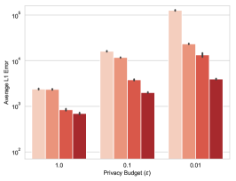
February     June     October                 

Figure 8: OptStream components analysis: Average $L_{1}$-error associated with the energy loads of the months of February, June, and October.

Figure 8 details the L1-errors associated with the private energy loads for the months of February, June, and October. This quantitative analysis further highlights the importance of the four components of the proposed OptStream algorithm. It illustrates a gradual error reduction of the framework when it adopts, in order, the perturbation step only, the perturbations and the optimization steps, the perturbation and the sampling with linear interpolation steps, and finally, all four steps.

6.3 Stream Data-Release in the $(w,\alpha)$-Indistinguishability Model

Having analyzed the algorithms in the $w$-privacy setting, this section illustrates the results of the private data streams released under the combined $w$-event and $\alpha$-indistinguishability models (see Section 5.1). The motivating application requires releasing the private data streams without disclosing chosen amounts of load changes within a time window. We thus analyze the results of privately releasing a stream of data under the $(w,\alpha)$-indistinguishability model and use an adapted version of OptStream, the Laplace mechanism, and the DFT algorithm. These versions recalibrate the noise required by the mechanisms to satisfy the $(w,\alpha)$-indistinguishability definition as detailed in Section 5.1.

Real                            Laplace                            DFT                        OptStream

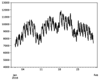
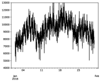
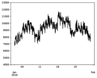
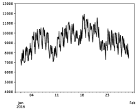
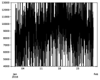
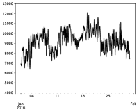
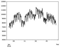
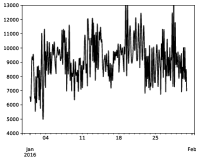
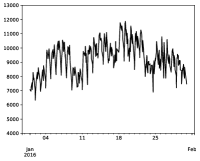
Figure 9: Real load consumption data for the Auvergne-Rhône-Alpes region in January 2016, and its private versions obtained using Laplace, DFT, and OptStream with privacy budget $\epsilon=1$ and $\alpha=10$ (top), $50$ (middle), and $100$ (bottom).

Figure 9 illustrates the real and private versions of the data stream for $w$-periods of size 48 (i.e., one day) given privacy budget of $\epsilon=1$ and indistinguishability parameter $\alpha=10$ (top row), $\alpha=50$ (middle row) and $\alpha=100$ (bottom row). Recall that the choice of the indistinguishability parameter $\alpha$ allows the data curator to ensure the protection of the observed increase/decrease power consumption up to $\alpha$ MegaWatts (MW), while the $w$-period specifies the length of the obfuscation period. The figure compares our proposed OptStream algorithm against the Laplace mechanism and DFT .

For DFT and OptStream, the experiments set the number of Fourier coefficients and sampling steps to $10$ (when $\alpha\leq 50$) and $5$ (when $\alpha=100$). As in the previous experiments, the privacy budget allocated to perform each measurement is divided equally. Finally, OptStream uses the same feature query set ${\mathscr{F}}$ used in the previous experiments. Figure 9 clearly illustrates that OptStream produces private streams that are more accurate than its competitors when visualized. This is especially evident for high indistinguishability parameters, when the Laplace mechanism can barely preserve any signal from the original data.

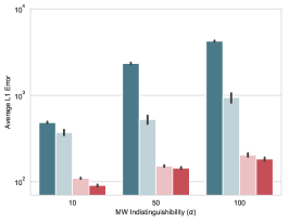
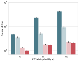
February     June     October                 

Figure 10: $L_{1}$-error analysis: Energy load stream data for the months of February, June, and October. The $y$-axis reports $\log_{10}$ errors averaged across the $L_{1}$ errors for each stream data $R\in{\mathscr{R}}$.

We now report the $L_{1}$-errors averaged for each $w$-period produced by the algorithms. Figure 10 reports the average results for each streaming region for the months of February, June, and October, at varying of the indistinguishability parameter $\alpha=\{10,50,100\}$ given a privacy budget $\epsilon=1.0$. Each histogram reports the log₁₀ value of the average error of 30 random trials. While all algorithms induce an $L_{1}$-error which increases as the indistinguishability level $\alpha$ increases, the figure highlights that OptStream consistently outperforms the other algorithms.

7 Discussion

One of the core advantages of the w-privacy model is that it provides flexibility regarding the size of the time frame to protect. OptStream exploits this flexibility to select a small set of representative points to sample and performs additional optimization over such values to redistribute noise and enhance accuracy. Practically, this means that the data stream needs to be batched in periods of $w$ times steps, each of which is privately released at once.

Recall that the privacy model adopted in this paper combines the $w$-privacy model (?) with the definition of $\alpha$-indistinguishability (?). The resulting $(w,\alpha)$-indistinguishability model allow us to protect events related to quantities which are not directly related to user identities but can be used a proxy to disclose a secret (e.g., a sensitive information) about a user. For instance, in our application domain, it is important to both protect the given stream from inferences about load increases or decreases–which are typically related to sensitive user activities–while also protecting the stream in an entire day.

While setting $w=1$ would allow to use OptStream to release the stream data online – without requiring batching –, this setting offers no room for OptStream to improve accuracy, since it would be similar to the Laplace mechanism. To the best of our knowledge, the only available algorithm that can release a private data stream online is PeGaSus (?). It uses a combination of the Laplace mechanism, a partitioning strategy to group values in contiguous time steps whose deviation is small, and a smoothing function. PeGaSus, was not introduced in the w-event model as it focuses on protecting data in a single time-step.

Real                         PeGaSus                   OptStream

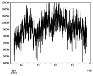
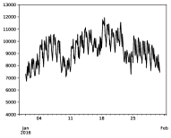
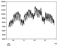
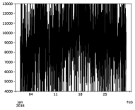
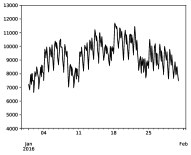
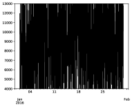
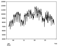
Figure 11: Real load consumption data for the Auvergne-Rhône-Alpes region in January 2016 (left), and its private versions obtained using PeGaSus (center), and OptStream (right) with privacy budget $\epsilon=1$ (top-row), $\epsilon=0.1$ (middle-row), and $\epsilon=0.01$ (bottom-row).

Despite the fact that the two algorithms were designed for solving different problems, we adapted PeGaSus to the $w$-privacy model and to satisfy the $(w,\alpha)$-indistinguishability and compare it against OptStream for completeness. Figure 11 illustrates a comparison of the algorithms on privately releasing load streams for the Auvergne-Rhône-Alpes region in January 2016. The real loads are highlighted in the first column, while their private counterparts are shown in the second and third columns. The figure compares our proposed OptStream (third column) against PeGaSus (second column) for indistinguishability parameters $\alpha=10$ (top rows) $\alpha=50$ (middle row) and $\alpha=100$ (bottom row), and fixed a privacy budget $\epsilon=1$. For PeGaSus, the privacy budget is divided equally for each time step in the $w$-period. Additionally, the experiments use the values of the meta-parameters indicated in the original paper (?). The settings for OptStream are the same as in the previous sections. Figure 11 clearly illustrates that OptStream produces private streams that are more accurate than those produced by PeGaSus, when the $(w,\alpha)$-indistinguishability model is adopted. It is an interesting research avenue to combine PeGaSus and OptStream.

8 Related Work

Continuous release of aggregated real-time data has been studied in previous work including (?, ?). Most of the state-of-the-art either focuses on event-level privacy on infinite streams (?) or on user-level privacy on finite streams (?). Dwork proposed an adaptation of differential privacy to a continuous observation setting (?). Her work focused on releasing bit-streams and proposed an algorithm for counting the number of 1s in the stream under event-level differential privacy. ? (?) proposed pan-privacy for estimating counts, moments, and heavy-hitters on data streams while preserving differential privacy even if the internal memory of the algorithms is observed by an attacker. ? (?) proposed the notion of $w$-event privacy to balance event-level and user-level privacy, trading off utility and privacy to protect event sequences within a time window of $w$ time steps. OptStream applies to the last model.

Within the differential privacy proposal for data streams that fit such model, ? (?) proposed Rescue DP, which is designed explicitly for spatiotemporal traces. PeGaSus (?) is another seminal work that allows to protect event privacy using a combination of perturbation, partitioning, and smoothing. The algorithm uses a combination of Laplace noise to perturb the data stream for privacy, a grouping strategy which incrementally partitions the space of observed data points by grouping points with small deviations, and a smoothing schema which is used to post-process the private data stream. Both algorithms rely on the idea of contiguous grouping time steps and average the perturbed data within every region in a group. We compared OptStream against PeGaSus, which is the state-of-the-art on private data-stream release and has been showed to be effective in several settings.

? (?) proposed an algorithm which perturbs a small number of Discrete Fourier Transform (DFT) coefficients of the entire time series and reconstructs a released version of the Inverse DFT series. While, in the original paper, the algorithm requires the entire time-series, such approach has been used for $w$-event privacy in the context of data streams (?). We also compare OptStream against DFT.

? (?) proposed Fast, an adaptive algorithm for private release of aggregate statistics which uses a combination of sampling and filtering. Their algorithm is based on user-level differential privacy, which is not comparable to the chosen model of $w$-event level differential privacy. Additionally, in their work, the authors compare the proposed approach against DFT (?) and, while showing improvements, the error remains within the same error magnitude of those produced by DFT. In contrast, our experimental analysis (Section 6) clearly illustrates that OptStream reduces the error of one order of magnitude when compared to DFT.

Finally, ? (?) focused on releasing prefix-sums of the streaming data counts while adopting an event-based privacy model. ? (?) also used an event-based model and proposed an algorithm for answering sliding window queries on data streams. The model adopted in their work is however incompatible with the privacy model adopted in this work, and hence we did not compare against such approaches.

9 Conclusions

This paper presented OptStream, a novel algorithm for privately releasing stream data in the $w$-event privacy model. OptStream is a 4-step procedure consisting of sampling, perturbation, reconstruction, and post-processing modules. The sampling module selects a small set of data points to measure privately in each period of interest. The perturbation module injects noise to the sampled data points to ensure privacy. The reconstruction module reconstructs the data points excluded from measurement from the perturbed sampled points. Finally, the post-processing module uses convex optimization over the private output of the previous modules, along with the private answers of additional queries on the data stream, to ensure consistency of quantities associated with salient features of the data. OptStream was evaluated on a real dataset from the largest transmission operator in Europe. Experimental results on multiple test cases show that OptStream improves the accuracy of the state-of-the-art by at least one order of magnitude in this application domain. The accuracy improvements are measured, not only in terms of the error distance to the original stream but also in the accuracy of a popular load forecasting algorithm trained on private data sub-streams. The results additionally show that OptStream exhibits similar benefits on hierarchical stream data which is also highly desirable in practice. Finally, the experimental analysis has demonstrated that both the adaptive sampling and post-processing optimization are critical in obtaining strong accuracy. Future work will be devoted to generalizing these results to the streaming setting where a data element is emitted at each time step.

References

- Alwan and Roberts Alwan, L. C., and Roberts, H. V. (1988). Time-series modeling for statistical process control. Journal of Business & Economic Statistics, 6(1), 87–95.
- Andrés, Bordenabe, Chatzikokolakis, and Palamidessi Andrés, M. E., Bordenabe, N. E., Chatzikokolakis, K., and Palamidessi, C. (2013). Geo-indistinguishability: Differential privacy for location-based systems. In Proceedings of the 2013 ACM SIGSAC conference on Computer & communications security, pp. 901–914. ACM.
- Bolot, Fawaz, Muthukrishnan, Nikolov, and Taft Bolot, J., Fawaz, N., Muthukrishnan, S., Nikolov, A., and Taft, N. (2013). Private decayed predicate sums on streams. In Proceedings of the 16th International Conference on Database Theory, pp. 284–295. ACM.
- Chan, Shi, and Song Chan, T.-H. H., Shi, E., and Song, D. (2011). Private and continual release of statistics. ACM Transactions on Information and System Security (TISSEC), 14(3), 26.
- Chatzikokolakis, Andrés, Bordenabe, and Palamidessi Chatzikokolakis, K., Andrés, M. E., Bordenabe, N. E., and Palamidessi, C. (2013). Broadening the scope of differential privacy using metrics. In International Symposium on Privacy Enhancing Technologies Symposium, pp. 82–102. Springer.
- Chen, Machanavajjhala, Hay, and Miklau Chen, Y., Machanavajjhala, A., Hay, M., and Miklau, G. (2017). Pegasus: Data-adaptive differentially private stream processing. In Proceedings of the 2017 ACM SIGSAC Conference on Computer and Communications Security, pp. 1375–1388. ACM.
- Cochrane Cochrane, J. H. (2005). Time series for macroeconomics and finance. Manuscript, University of Chicago.
- Ding, Kulkarni, and Yekhanin Ding, B., Kulkarni, J., and Yekhanin, S. (2017). Collecting telemetry data privately. In Advances in Neural Information Processing Systems, pp. 3574–3583.
- Dwork Dwork, C. (2010). Differential privacy in new settings. In Proceedings of the twenty-first annual ACM-SIAM symposium on Discrete Algorithms, pp. 174–183. SIAM.
- Dwork, McSherry, Nissim, and Smith Dwork, C., McSherry, F., Nissim, K., and Smith, A. (2006). Calibrating noise to sensitivity in private data analysis. In TCC, Vol. 3876, pp. 265–284. Springer.
- Dwork, Naor, Pitassi, and Rothblum Dwork, C., Naor, M., Pitassi, T., and Rothblum, G. N. (2010). Differential privacy under continual observation. In Proceedings of the forty-second ACM symposium on Theory of computing, pp. 715–724. ACM.
- Dwork and Roth Dwork, C., and Roth, A. (2013). The algorithmic foundations of differential privacy. Theoretical Computer Science, 9(3-4), 211–407.
- Fan and Xiong Fan, L., and Xiong, L. (2014). An adaptive approach to real-time aggregate monitoring with differential privacy. IEEE Transactions on Knowledge and Data Engineering, 26(9), 2094–2106.
- Fan, Xiong, and Sunderam Fan, L., Xiong, L., and Sunderam, V. (2013). Fast: differentially private real-time aggregate monitor with filtering and adaptive sampling. In Proceedings of the 2013 ACM SIGMOD International Conference on Management of Data, pp. 1065–1068. ACM.
- Fanti, Pihur, and Erlingsson Fanti, G., Pihur, V., and Erlingsson, Ú. (2016). Building a rappor with the unknown: Privacy-preserving learning of associations and data dictionaries. Proceedings on Privacy Enhancing Technologies, 2016(3), 41–61.
- Fawaz and Shin Fawaz, K., and Shin, K. G. (2014). Location privacy protection for smartphone users. In Proceedings of the 2014 ACM SIGSAC Conference on Computer and Communications Security, pp. 239–250. ACM.
- Fioretto, Lee, and Van Hentenryck Fioretto, F., Lee, C., and Van Hentenryck, P. (2018). Constrained-based differential privacy for mobility services. In Proceedings of the 17th International Conference on Autonomous Agents and MultiAgent Systems, AAMAS, pp. 1405–1413.
- Hardt and Rothblum Hardt, M., and Rothblum, G. N. (2010). A multiplicative weights mechanism for privacy-preserving data analysis. In Foundations of Computer Science. IEEE.
- Hipel and McLeod Hipel, K. W., and McLeod, A. I. (1994). Time series modelling of water resources and environmental systems, Vol. 45. Elsevier.
- Kellaris, Papadopoulos, Xiao, and Papadias Kellaris, G., Papadopoulos, S., Xiao, X., and Papadias, D. (2014). Differentially private event sequences over infinite streams. Proceedings of the VLDB Endowment, 7(12), 1155–1166.
- Koufogiannis, Han, and Pappas Koufogiannis, F., Han, S., and Pappas, G. J. (2015). Optimality of the laplace mechanism in differential privacy. arXiv preprint arXiv:1504.00065.
- Mir, Muthukrishnan, Nikolov, and Wright Mir, D., Muthukrishnan, S., Nikolov, A., and Wright, R. N. (2011). Pan-private algorithms via statistics on sketches. In Proceedings of the thirtieth ACM SIGMOD-SIGACT-SIGART symposium on Principles of database systems, pp. 37–48. ACM.
- Nemirovski Nemirovski, A. (2004). Interior point polynomial time methods in convex programming. Tech. rep. ISYE 8813, Georgia Institute of Technology, Atlanta, GA.
- Nogales, Contreras, Conejo, and Espínola Nogales, F. J., Contreras, J., Conejo, A. J., and Espínola, R. (2002). Forecasting next-day electricity prices by time series models. IEEE Transactions on power systems, 17(2), 342–348.
- Ochoa and Harrison Ochoa, L. F., and Harrison, G. P. (2011). Minimizing energy losses: Optimal accommodation and smart operation of renewable distributed generation. IEEE Transactions on Power Systems, 26(1), 198–205.
- Rastogi and Nath Rastogi, V., and Nath, S. (2010). Differentially private aggregation of distributed time-series with transformation and encryption. In Proceedings of the 2010 ACM SIGMOD International Conference on Management of data, pp. 735–746. ACM.
- Wang, Zhang, Lu, Wang, Qin, and Ren Wang, Q., Zhang, Y., Lu, X., Wang, Z., Qin, Z., and Ren, K. (2016). Rescuedp: Real-time spatio-temporal crowd-sourced data publishing with differential privacy. In INFOCOM 2016-The 35th Annual IEEE International Conference on Computer Communications, IEEE, pp. 1–9. IEEE.
- Zhang Zhang, G. P. (2003). Time series forecasting using a hybrid arima and neural network model. Neurocomputing, 50, 159–175.